Abstract

Two coupled oscillators provide a mathematical instrument for solving many problems in modern physics, including squeezed states of light and Lorentz transformations of quantum bound states. The concept of entanglement can also be studied within this mathematical framework. For the system of two entangled photons, it is of interest to study what happens to the remaining photon if the other photon is not observed. It is pointed out that this problem is an issue of Feynman’s rest of the universe. For quantum bound-state problems, it is pointed out the longitudinal and time-like coordinates become entangled when the system becomes boosted. Since time-like oscillations are not observed, the problem is exactly like the two-photon system where one of the photons is not observed. While the hadron is a quantum bound state of quarks, it appears quite differently when it moves rapidly than when it moves slowly. For slow hadrons, Gell-Mann’s quark model is applicable, while Feynman’s parton model is applicable to hadrons with their speeds close to that of light. While observing the temperature dependence of the speed, it is possible to explain the quark-to-parton transition as a phase transition.

to be published in the Physical Science International Journal.

1 Introduction

When Einstein developed his special relativity in 1905, he worked out a transformation law for a point particle. Presumably he was aware that the hydrogen atom consists of one electron circling around a proton. However, he did not mention the question of how the electron orbit appears to a moving observer.

Since then, many authors had ideas about a possible elliptic deformation of the orbit as described in Fig. 1. However, quantum mechanics made this concept obsolete. The hydrogen orbit was replaced by a standing wave. Thus, the question is how the standing wave looks to a moving observer.

For thirty six years from 1927 to 1963, Paul A. M. Dirac was occupied with this problem. In 1927 [1], Dirac noted that there is an uncertainty relation between time and energy variables but there are no excitations along the time axis. He stated that this space-time asymmetry makes it difficult to make quantum mechanics consistent with relativity.

In 1945 [2], Dirac attempted to use a four-dimensional Gaussian form to construct a representation of the Lorentz group, but did not reach specific conclusions. In 1949 [3], Dirac stated that the construction of a relativistic dynamics is equivalent to constructing a representation of the ten-parameter Poincaré group. He noted difficulties in doing so.

In 1963 [4], Dirac published a paper on the symmetry of two harmonic oscillators, in which he constructed a set of generators for the deSitter group $O(3,2)$. This paper gives an indication that it is possible to use harmonic oscillators to construct the desired representations for the Poincaré group, such as Wigner’s little groups [5]. Wigner’s little groups are the subgroups of the Lorentz group which dictate the internal space-time symmetries of particles in the Lorentz-covariant world [6].

In this paper, we construct standing waves which can be Lorentz-boosted using harmonic-oscillator wave functions. In so doing, we face the problem of the time-separation variable. Standing waves are of course for bound states.

For the bound-state problem, the space coordinate gives the space separation between two constituent particles, like the Bohr radius which measures the distance between the proton and electron in the hydrogen atom. Then there comes the question of the time variable in the bound-state system. This is a time-separation variable not contained in the Schrödinger picture of quantum mechanics. On the other hand, this time separation becomes prominent when the system is boosted, and it becomes as big as the space separation if the system moves with a speed close to that of light.

Indeed, it is a challenge how to take into account this time separation variable. In order to address this question, we note first that Dirac raised the question of time-energy uncertainty relation in 1927 when the present form of quantum mechanics was inaugurated [1]. Dirac noted however that there are no excitations along the time-like direction.

In this paper, we explain in detail how this time-separation variable can be incorporated into a Lorentz covariant formalism. In spite of its prominence in the covariant formalism, this variable does not exist in the Schrödinger picture of quantum mechanics. There are no measurement theories to deal with this problem.

If the variable exists and we are not able to measure it, the result is an increase in entropy and a temperate rise. We treat this problem systematically with the existing rules of quantum mechanics and relativity. It is convenient to explain this process by using the concepts of entanglement, decoherence, and Feynman’s rest of the universe.

In Sec. 2, we start with the Hamiltonian for two independent variables. We then couple the system by making a canonical transformation. In Sec. 3, the Lorentz covariant harmonic oscillator is presented. This formalism takes into account Dirac’s concerns mentioned in his papers [1, 2, 3].

In Sec. 4, we discuss how the space-time variables become entangled when the quantum bound state is boosted. It is shown that this entanglement leads to an increase in entropy and a rise in temperature. In Sec. 5, it is noted that the hadron appears quite differently when it moves rapidly than when it moves slowly. For slow hadrons, Gell-Mann’s quark model is applicable, while Feynman’s parton model is applicable to hadrons with their speeds close to that of light. While observing the temperature dependence of the speed, we can explain the quark-to-parton transition as a phase transition.

In combining quantum mechanics with special relativity, quantum field theory occupies a very importance place. In the Appendix, we discuss where QFT stands with respect to our work.

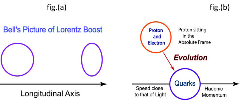
Figure 1: Hydrogen atom or standing wave in the Lorentz-covariant world. The Lorentz contraction leads us to sketch an elliptic electron orbit for the moving hydrogen atom [7], as shown in fig.(a). This became an outdated concept after 1927. The electron orbit became a standing wave. The issue is how to Lorentz-boost the standing wave. Since the hydrogen atom cannot be accelerated, we have to study the standing wave for the proton, as illustrated in fig.(b). The proton is a bound state of quarks. The energy of the proton from CERN’s LHC is 4,000 times its mass, and its speed is extremely close to that of light.

2 Coupled Oscillators and Entangled Oscillators

Let us start with two uncoupled oscillators. The Hamiltonian for this system is

$$H=\frac{1}{2}\left(p_{1}^{2}+x_{1}^{2}\right)+\frac{1}{2}\left(p_{2}^{2}+x_{2}^{2}\right),$$ (1)

where

$$p_{1}=-i\frac{\partial}{\partial x_{1}},\qquad p_{2}=-i\frac{\partial}{\partial x_{2}}.$$

If we introduce the variables

$$x_{+}=\frac{x_{1}+x_{2}}{\sqrt{2}},\qquad x_{-}=\frac{x_{1}-x_{2}}{\sqrt{2}},$$

$$p_{+}=\frac{p_{1}+p_{2}}{\sqrt{2}},\qquad p_{-}=\frac{p_{1}-p_{2}}{\sqrt{2}}.$$ (2)

The Hamiltonian becomes

$$H=\frac{1}{2}\left[p_{+}^{2}+x_{+}^{2}\right]+\frac{1}{2}\left[p_{-}^{2}+x_{-}^{2}\right].$$ (3)

The resulting ground-state wave function is

$$\psi\left(x_{1},x_{2}\right)=\frac{1}{\sqrt{\pi}}\exp{\left[-\frac{1}{2}\left(x_{+}^{2}+x_{-}^{2}\right)\right]}$$ (4)

This aspect of the two uncoupled oscillators is well known. The question is what happens they become coupled.

2.1 Canonical Transformation

The canonical way to couple these two oscillators is to apply the coordinate transformation

$$\pmatrix{x_{+}\cr p_{-}}\rightarrow e^{-\eta}\pmatrix{x_{+}\cr p_{-}},\qquad\pmatrix{x_{-}\cr p_{+}}\rightarrow e^{\eta}\pmatrix{x_{-}\cr p_{+}}.$$ (5)

This transformation leads to the Hamiltonian of the form

$$H_{\eta}=\frac{1}{2}\left[e^{2\eta}p_{+}^{2}+e^{-2\eta}x_{+}^{2}\right]+\frac{1}{2}\left[e^{-2\eta}p_{-}^{2}+e^{2\eta}x_{-}^{2}\right],$$ (6)

and the wave function of Eq.(4) to

$$\psi_{\eta}\left(x_{1},x_{2}\right)=\frac{1}{\sqrt{\pi}}\exp{\left\{-\frac{1}{4}\left[e^{-2\eta}\left(x_{1}+x_{2}\right)^{2}+e^{2\eta}\left(x_{1}-x_{2}\right)^{2}\right]\right\}}.$$ (7)

This canonical transformation is illustrated in Fig. 2. From this figure, it is quite safe to say that the canonical transformation in this case is a “squeeze” transformation.

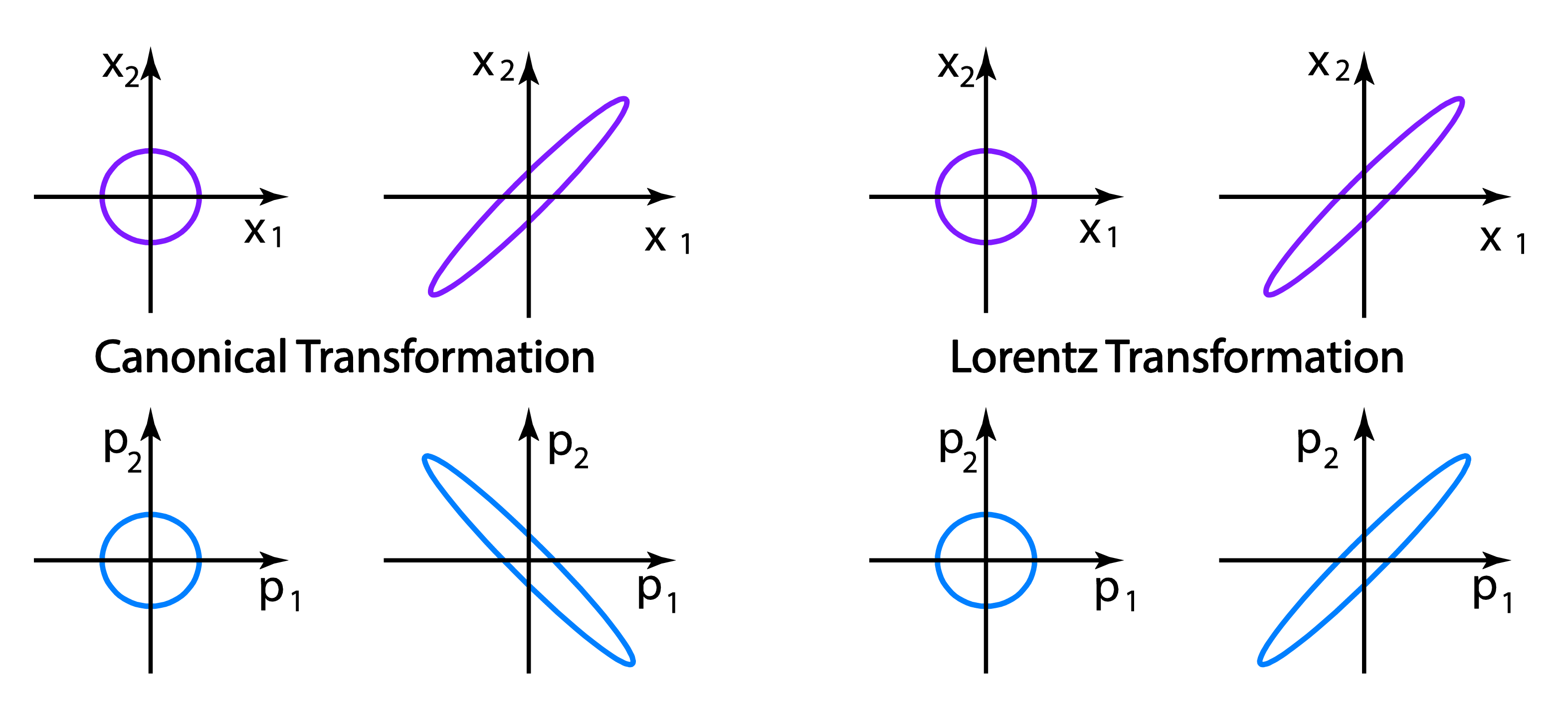
Figure 2: Canonical and Lorentz transformations. In the canonical transformation, the momentum coordinates and are inversely proportional to their conjugate coordinates. In the Lorentz transformation, the momentum space and momentum coordinate transform in the same way, as will be seen in Fig. 10.

2.2 Lorentz Transformation

While the Hamiltonians of Eq.(3) and Eq.(6) take two different forms, we are led to the question of whether there is a quantity invariant under this canonical transformation. For this purpose, let us consider the Hamiltonian of the form

$$H_{inv}=\frac{1}{2}\left(p_{1}^{2}+x_{1}^{2}\right)-\frac{1}{2}\left(p_{2}^{2}+x_{2}^{2}\right).$$ (8)

This is the expression for the energy of the first oscillator minus that of the second oscillator in this two-oscillator system. If we write this form in terms of the $x_{\pm}$ and $p_{\pm}$ variables,

$$H_{inv}=p_{+}p_{-}+x_{+}x_{-}.$$ (9)

This form is invariant under the canonical transformation of Eq.(5).

In addition, let us consider the transformation

$$\pmatrix{x_{+}\cr p_{+}}\rightarrow e^{-\eta}\pmatrix{x_{+}\cr p_{+}},\qquad\pmatrix{x_{-}\cr p_{-}}\rightarrow e^{\eta}\pmatrix{x_{-}\cr p_{-}}.$$ (10)

This is not a canonical transformation. The space and momentum variables are transformed in the same way, as in the case of Einstein’s Lorentz boost. Thus, we choose to call this transformation the Lorentz transformation, and illustrated it in Fig. 2.

The invariant Hamiltonian was considered first by Yukawa [8], and then by Feynman et al. [9].

2.3 Entangled Oscillators

As was discussed in the literature for several different purposes [6, 10, 11, 12, 13], this wave function can be expanded as

$$\psi_{\eta}\left(x_{1},x_{2}\right)={1\over\cosh\eta}\sum_{k}(\tanh\eta)^{k}\phi_{k}(x_{1})\phi_{k}(x_{2}),$$ (11)

where $\phi_{k}(x)$ is the normalized harmonic oscillator wave function for the $k^{th}$ excited state, and it takes the form.

$$\phi_{k}(x)=\left(1\over\sqrt{\pi}n!2^{k}\right)^{1/2}H_{k}(x)\exp{\left(\frac{-x^{2}}{2}\right)},$$ (12)

where $H_{k}$ is the Hermite polynomial of the $k^{th}$ order.

The harmonic oscillator states are also used as photon-number states in quantum electrodynamics. The expansion of Eq.(11) serves as the mathematical basis for two-photon coherent states or squeezed states of light in quantum optics [4, 14, 15, 16, 17], among other applications. More recently, this expansion is called the entangled state of two photons [11]. Thus, it is appropriate to call the expression of Eq.(11) the entangled state of two oscillators [12].

3 Harmonic Oscillators in the Lorentz-covariant World

Paul A. M. Dirac is known to us through the Dirac equation for spin-1/2 particles. However, his main interest was in foundational problems. First, Dirac was never satisfied with the probabilistic formulation of quantum mechanics. This is still one of the hotly debated subjects in physics. Second, if we tentatively accept the present form of quantum mechanics, Dirac was insisting that it has to be consistent with special relativity. He wrote several important papers on this subject. Let us look at some of his papers. Among them were

• In 1927 [1], Dirac published a paper on the time-energy uncertainty relation. He noted there that the time-energy relation is necessarily a c-number uncertainty relation because there are no excitations along the time-like dimension. He noted further this space-time asymmetry makes it difficult to make quantum mechanics compatible with special relativity.

• In his paper of 1945 [2], Dirac attempted to use harmonic oscillator wave functions to construct a representation of the Lorentz group. He knew quantum mechanics is the physics of harmonic oscillators and special relativity is the physics of the Lorentz group. For this purpose, he wrote down the Gaussian factor

  $$\exp\left\{-{1\over 2}\left(x^{2}+y^{2}+z^{2}+t^{2}\right)\right\}.$$ (13)

  Since the oscillator wave function is separable, we can consider only

  $$\exp\left\{-{1\over 2}\left(z^{2}+t^{2}\right)\right\},$$ (14)

  when Lorentz boosts are made along the $z$ direction. This form is not invariant under the boost. Furthermore, it vanishes when the $t$ variable becomes $\pm\infty.$ Does this mean that the world starts with zero in the remote past and vanishes also in the future?

• In his 1949 paper [3], Dirac introduced the ten generators of the Poincaré group, and stated that the task of constructing a Lorentz-covariant quantum mechanics is equivalent to constructing a representation of the Poincaré group. In order to make contact with the Schrödinger form of quantum mechanics, he considered three different forms of constraint, which are called instant form, front form, and point form. Dirac then noted the difficulties in constructing a desired representation.

  Also in this paper, Driac introduced his light-cone coordinate system in order to elaborate on his front form of quantum mechanics.

We propose here to construct Dirac’s desired quantum mechanics by supplementing the ideas missing in his papers. First of all, let us look at Gaussian form of Eq.(13). By writing down this Gaussian form, Dirac was clearly interested in standing waves. Standing waves in quantum mechanics require boundary conditions. The issue is then how those boundary conditions appear to a moving observer. We can take care of this problem if we use harmonic oscillators with their built-in boundary conditions, as Dirac did in his 1945 paper [2] without mentioning it.

However, in writing down the Gaussian form, Dirac forgot to mention that the space and time variables are space and time separation variables. For instance, the Bohr radius measures the space separation between the proton and electron. Thus the $t$ variable in the Gaussian form is the time separation variable which vanishes if the hydrogen atom is at rest. However, this time separation becomes prominent when the hydrogen atom moves, as illustrated in Fig. 3.

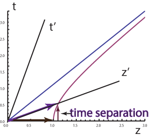
Figure 3: Time separation in relativity. In relativity, there is a time separation wherever there is a space separation. The Bohr radius is a space separation. It was Feynman et al. [9] who pointed out the existence of this variable, but they said they did not know what to do with it in their oscillator formalism.

Thus, the $t$ variable in the Gaussian form does not say the system becomes zero in the remote past or remote future. This variable is hidden in the Schrödinger form of quantum mechanics. The question then is how to hide this variable when we extract the Schrödinger picture of quantum mechanics from Dirac’s Lorentz-covariant form.

In his 1949 paper [3], Dirac’s states his constraints are not consistent with the Poincaré covariance. However, Dirac overlooked Wigner’s work on the little groups which dictate internal space-time symmetries of particles [5]. The little groups are maximal subgroups of the Lorentz group whose transformations leave the four-momentum of a given particle invariant. Thus, these subgroups cannot satisfy the full symmetries of the Poincaré group.

Let us go back to the Gaussian form of Eq.(13) again. It clearly indicates that there is an uncertainty relation along the time direction, but Dirac’s instant form forbids excitations along this axis. This aspect is perfectly consistent with the c-number time-energy uncertainty relation Dirac mentioned in his 1927 paper [1].

If we make up for all the soft spots in Dirac’s papers mentioned in this section, we end up with an oscillator model of Lorentz-covariant quantum mechanics illustrated in Fig. 4.

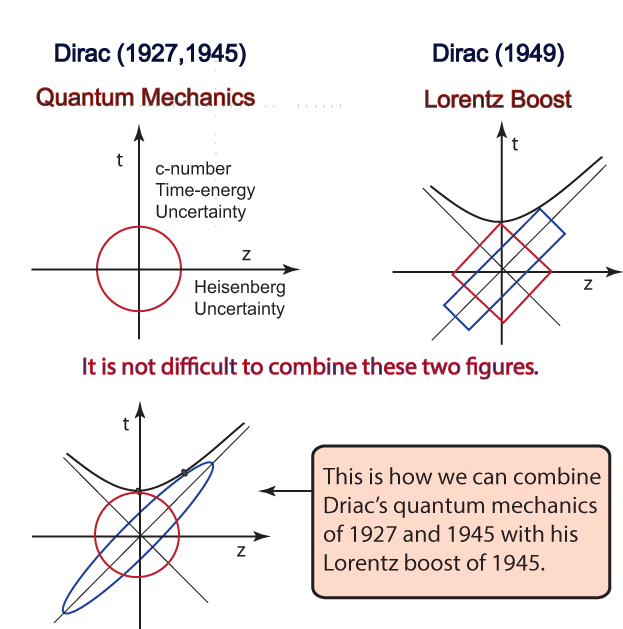
Figure 4: Space-time picture of bound-state quantum mechanics. If we combine Dirac’s 1927 and 1945 papers [1, 2], we end up an oscillator wave function without excitations along the time axis. Dirac’s 1949 paper [3] gives a squeeze picture of the Lorentz boost. It is then not difficult to combines these two pictures to construct a Lorentz-covariant picture of the wave function.

In Fig. 4, we start with the Gaussian expression given in Eq. 14. This expression is not invariant under the Lorentz boost along the $z$ direction, which can be written as

$$\pmatrix{z^{\prime}\cr t^{\prime}}=\pmatrix{\cosh\eta&\sinh\eta\cr\sinh\eta&\cosh\eta}\pmatrix{z\cr t},$$ (15)

with

$$\tanh(\eta)=v/c,$$ (16)

where $v$ is the velocity of the boost.

If we use Dirac’s light-cone variables defined as [3],

$$u=(z+t)/\sqrt{2},\qquad v=(z-t)/\sqrt{2},$$ (17)

the boost transformation of Eq.(15) takes the form

$$u^{\prime}=e^{\eta}u,\qquad v^{\prime}=e^{-\eta}v.$$ (18)

The $u$ variable becomes expanded while the $v$ variable becomes contracted, as is illustrated in Fig. 4. Their product

$$uv={1\over 2}(z+t)(z-t)={1\over 2}\left(z^{2}-t^{2}\right)$$ (19)

remains invariant.

In terms of these variables, the Gaussian form can be written as

$$\exp{\left\{-{1\over 2}\left(u^{2}+v^{2}\right)\right\}}.$$ (20)

If we apply the Lorentz boost on this function, it becomes

$$\exp{\left\{-{1\over 2}\left(e^{-2\eta}u^{2}+e^{2\eta}v^{2}\right)\right\}}.$$ (21)

In this way, the harmonic oscillator wave function becomes Lorentz-boosted. As in the case of the canonical transformation of Fig. 2, the Lorentz boost is a squeeze transformation. Thus, we can study the Lorentz boost of the oscillator wave functions in terms of those in the system of coupled oscillators.

3.1 Feynman’s Oscillators

In his invited talk at the 1970 spring meeting of the American Physical Society held in Washington, DC (U.S.A.), Feynman noted first that the observed hadronic mass spectra are consistent with the degeneracy of three-dimensional harmonic oscillators. Furthermore, he stressed that Feynman diagrams are not necessarily suitable for relativistic bound states and that we should try harmonic oscillators. Feynman’s point was that, while plane-wave approximations in terms of Feynman diagrams work well for relativistic scattering problems, they are not applicable to bound-state problems. We can summarize what Feynman said in Fig. 5. The content of his talk was published in 1971 by Feynman, Kislinger, and Ravndal [9].

They use the simplest hadron consisting of two quarks bound together with an attractive force, and consider their space-time positions $x_{a}$ and $x_{b}$, and use the variables

$$X=(x_{a}+x_{b})/2,\qquad x=(x_{a}-x_{b})/2\sqrt{2}.$$ (22)

The four-vector $X$ specifies where the hadron is located in space and time, while the variable $x$ measures the space-time separation between the quarks. According to Einstein, this space-time separation contains a time-like component which actively participates as in Eq.(15), if the hadron is boosted along the $z$ direction. This aspect of Einstein’s special relativity is illustrated in Fig. 3.

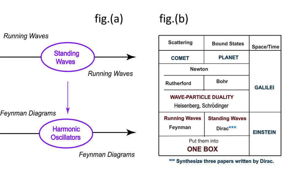
Figure 5: Feynman’s suggestion for combining quantum mechanics with special relativity. Feynman diagrams work for running waves, and they provide a satisfactory interpretation of scattering states in Einstein’s world. For standing waves trapped inside a hadron, Feynman suggested harmonic oscillators as the first step, as illustrated in fig.(a). From his suggestion, we can construct a historical perspective starting from comets and planets, as shown in fig.(b). Dirac’s three papers are discussed in Sec. 3. It has been shown by Han et al. in 1981 that the covariant oscillator formalism shares the same set of physical principles as Feynman diagrams for scattering problems [18].

For the internal space-time separation coordinates, Feynman et al. start with the Lorentz-invariant differential equation [9]

$$\frac{1}{2}\left(x^{2}_{\mu}-{\partial^{2}\over\partial x_{\mu}^{2}}\right)\psi(x)=\lambda\psi(x),$$ (23)

and write down their solutions. We would like to point out that those solutions are not compatible with the existing principle of physics, but they can be modified so that they are.

Since this oscillator equation is separable in the Cartesian coordinate system, and since the transverse components are not affected by Lorentz boost, we can drop the $x$ and $y$ components, and write Eq.(23) as

$$\frac{1}{2}\left\{\left[z^{2}-\left(\frac{\partial}{\partial z}\right)^{2}\right]-\left[t^{2}-\left(\frac{\partial}{\partial t}\right)^{2}\right]\right\}\psi(z,t)=\lambda\psi(z,t).$$ (24)

Here, the $z$ and $t$ variables are the space-time separation variables respectively. This partial differential equation has many different solutions depending on the choice of separable variables and boundary conditions. Feynman et al. chose the solutions with the Gaussian form

$$\exp{\left\{-{1\over 2}\left(z^{2}-t^{2}\right)\right\}},$$ (25)

as the ground-state wave function. This form is invariant under Lorentz boosts along the $z$ direction, but is not normalizable in the $t$ variable. For this reason, they drop this variable by setting $t=0$. In so doing they are destroying the Lorentz invariance they insisted on initially.

In their paper, Feynman et al. studied in detail the degeneracy of the three-dimensional harmonic oscillators, and compared their results with the observed experimental data. Their work is complete and thorough, and is consistent with the $O(3)$-like symmetry dictated by Wigner’s little group for massive particles [5, 6]. Yet, they make an apology that the symmetry is not that of $O(3,1)$. This unnecessary apology causes confusion not only to the readers but also to the authors themselves.

3.2 Lorentz-covariant Harmonic Oscillators

On the other hand, as was noted earlier [8], the Gaussian form of Eq.(14) also satisfies the Lorentz-invariant differential equation of Eq.(24). This form is not Lorentz-invariant but becomes Lorentz-squeezed according to Eq.(21).

In order to study whether the c-number time-energy uncertainty relation is consistent with Wigner’s $O(3)$-like little group for a massive particle, let us go back to the frame where the hadron is at rest. If we take into account the $x,y,$ and $z$ variables, it is possible to construct oscillator wave functions satisfying the $O(3)$ symmetry, with their proper angular momentum quantum numbers. This wave function should take the form

$$\psi(x,y,z,t)=\psi(x,y,z)\left[\left(\frac{1}{\pi}\right)^{1/4}\exp{\left(\frac{-t^{2}}{2}\right)}\right],$$ (26)

without time-like excitations [19]. The wave function $\psi(x,y.z)$ can be written in terms of the spherical variables [6]. Since the oscillator equation is separable in the Cartesian coordinate system, this wave function can also be written in terms of the Hermite polynomials. Here again, the transverse variables $x$ and $y$ are not affected by the boost along the $z$ direction, the wave function of interest can be written as

$$\psi^{n}(z,t)=\phi_{n}(z)\left[\left(\frac{1}{\pi}\right)^{1/4}\exp{\left(\frac{-t^{2}}{2}\right)}\right],$$ (27)

where $\phi_{n}(z)$ is for the $n^{th}$ excited oscillator state, given in Eq.(12). When the system is at rest, the full wave function is

$$\psi_{0}^{n}(z,t)=\left[1\over\pi n!2^{n}\right]^{1/2}H_{n}(z)\exp{\left\{-\left(\frac{z^{2}+t^{2}}{2}\right)\right\}}.$$ (28)

The subscript $0$ means that the wave function is for the hadron at rest.

We are now interested in boosting this wave function, and it is convenient to use the light-cone variables given in Eq.(17). In terms of these variables, the rest-frame wave function can be written as

$$\psi_{0}^{n}(z,t)=\left[1\over\pi n!2^{n}\right]^{1/2}H_{n}\left({u+v\over\sqrt{2}}\right)\exp{\left\{-\left(\frac{u^{2}+v^{2}}{2}\right)\right\}},$$ (29)

If the system is boosted, the wave function becomes

$$\psi_{\eta}^{n}(z,t)=\left[1\over\pi n!2^{n}\right]^{1/2}H_{n}\left({e^{-\eta}u+e^{\eta}v\over\sqrt{2}}\right)\exp{\left\{-\left(\frac{e^{-2\eta}u^{2}+e^{2\eta}v^{2}}{2}\right)\right\}}.$$ (30)

It is interesting that these wave functions satisfy the orthogonality condition [20].

$$\int\psi^{n}_{0}(z,t)\psi^{m}_{\eta}(z,t)dzdt=\left(\sqrt{1-\beta^{2}}\right)^{n}\delta_{nm},$$ (31)

where $\beta=\tanh\eta$. This orthogonality relation is illustrated in Fig. 6. The physical interpretation of this in terms of Lorentz contractions is given in our book [6], but it seems to require further investigation.

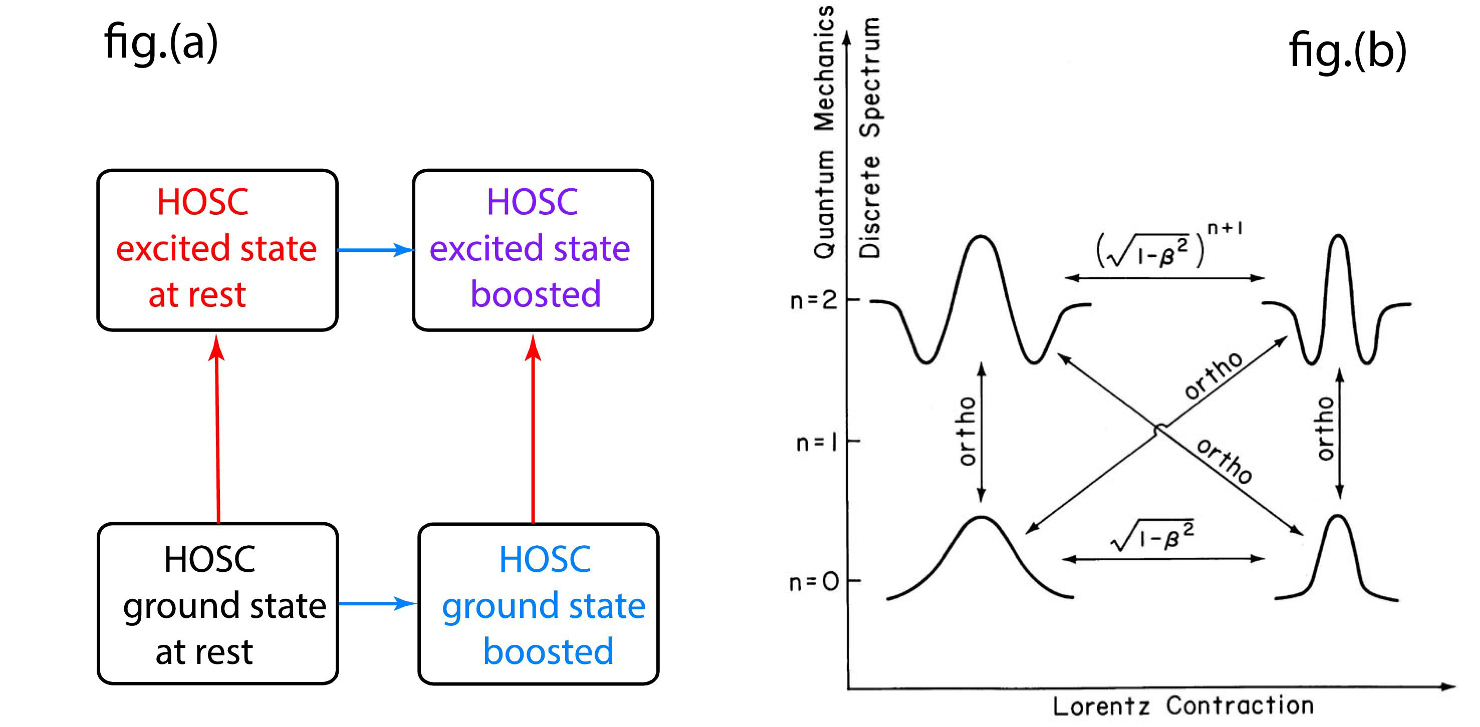
Figure 6: Orthogonality relations for covariant oscillator wave functions. The orthogonality relations remain invariant under Lorentz boosts, as shown in fig.(a). Their inner products have the Lorentz-contraction property given in fig.(b).

4 Entangled Space and Time

As was discussed in the literature for several different purposes, the Lorentz-boosted wave function of Eq.(30) can be expanded as [6, 21, 22]

$$\psi_{\eta}^{n}(z,t)=\left(\frac{1}{\cosh\eta}\right)^{(n+1)}\sum_{k}\left[\frac{(n+k)!}{n!k!}\right]^{1/2}(\tanh\eta)^{k}\phi_{n+k}(z)\phi_{n}(t).$$ (32)

For the ground state with $n=0$, this expansion becomes

$$\psi_{\eta}(z,t)={1\over\cosh\eta}\sum_{k}(\tanh\eta)^{k}\phi_{k}(z)\phi_{k}(t),$$ (33)

This expansion is identical to that for the coupled oscillators if $z$ and $t$ are replaced by $x_{1}$ and $x_{2}$ respectively. Indeed, this is the formula for the space-time entangled state of the ground-state oscillator with the c-number time-energy uncertainty state.

Let us go to the expansion of Eq.(32). We are justified to call this formula the entangled state of the $n^{th}$ excited state with the Gaussian form for the c-number time-energy uncertainty relation.

If the system is at rest, this time distribution can be separated from the rest, and we can recover Schrödinger’s quantum mechanics without the time-separation variable. If the system moves with non-zero value of $\eta$, this time-separation variable is entangled with the Schrödinger wave functions. What should we do?

In his book on statistical mechanics [23], Feynman makes the following statement about the density matrix.

When we solve a quantum-mechanical problem, what we really do is divide the universe into two parts - the system in which we are interested and the rest of the universe. We then usually act as if the system in which we are interested comprised the entire universe. To motivate the use of density matrices, let us see what happens when we include the part of the universe outside the system.

Figure 7 illustrates the time-separation variable belonging to Feynman’s rest of the universe. If we do not observe the variable in the rest of the universe, it causes an increase in entropy.

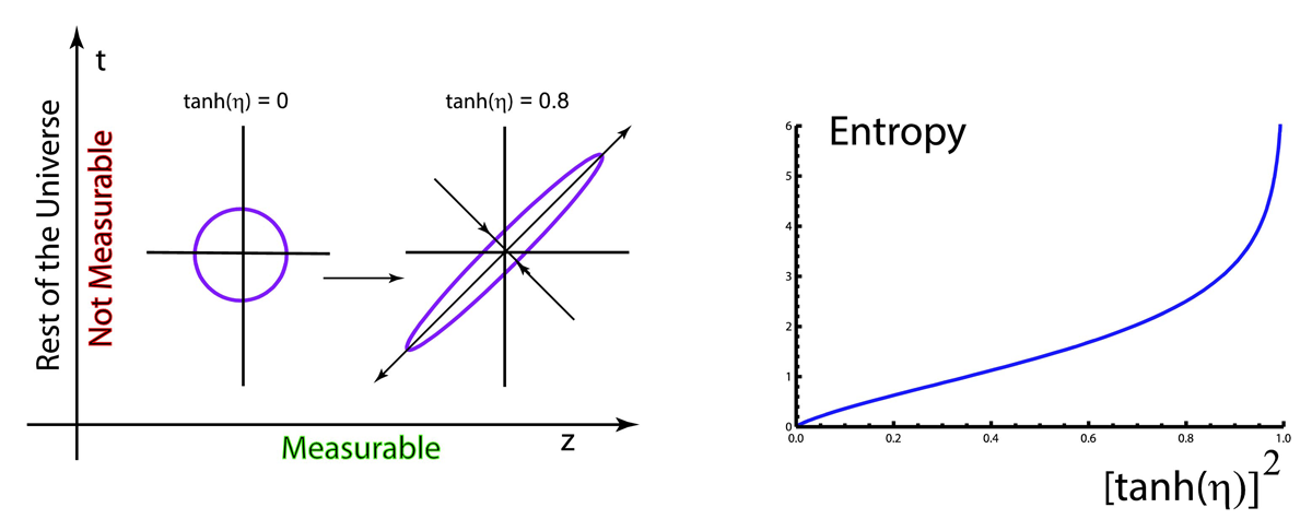
Figure 7: Localization property in the $zt$ plane. When the hadron is at rest, the Gaussian form is concentrated within a circular region specified by $(z+t)^{2}+(z-t)^{2}=1.$ As the hadron gains speed, the region becomes deformed to $e^{-2\eta}(z+t)^{2}+e^{2\eta}(z-t)^{2}=1.$ Since it is not possible to make measurements along the $t$ direction, we have to deal with information that is less than complete. This does not cause problems when the hadron is at rest, because the $t$ dependence in the density matrix is separable and can be integrated out. When the $t$ separation is not measured as in the case of the Schrödinger quantum mechanics, the entropy of the system becomes non-zero and becomes increased as the hadron gains speed.

4.1 Entropy and Lorentz Transformations

If the $z$ and $t$ variables are both measurable, we can construct the density matrix

$$\rho_{\eta}^{n}(z,t;z^{\prime},t^{\prime})=\psi_{\eta}^{n}(z,t)\left(\psi_{\eta}^{n}(z^{\prime},t^{\prime})\right)^{*},$$ (34)

from Eq.(27). Since the wave functions in the present paper are all real, we shall hereafter drop the $*$ sign for complex conjugate.

This form satisfies the pure-state condition $\rho^{2}=\rho$ which can be written explicitly as

$$\rho_{\eta}^{n}(z,t;z^{\prime},t^{\prime})=\int\rho_{\eta}^{n}(z,t;z",t")\rho_{\eta}^{n}(z",t";z^{\prime},t^{\prime})dz"dt".$$ (35)

However, there are at present no measurement theories which accommodate the time-separation variable $t$. Thus, we can take the trace of the $\rho$ matrix with respect to the $t$ variable. Then the resulting density matrix is

$$\rho_{\eta}^{n}(z,z^{\prime})=\int\psi_{\eta}^{n}(z,t)\psi_{\eta}^{n}(z^{\prime},t)dt$$

$$\hskip 22.76219pt=\left(\frac{1}{\cosh\eta}\right)^{2(n+1)}\sum_{k}\frac{(n+k)!}{n!k!}(\tanh\eta)^{2k}\phi_{n+k}(z)\phi_{k+n}(z^{\prime}).$$ (36)

The trace of this density matrix is one, but the trace of $\rho^{2}$ is less than one, as

$$Tr\left(\rho^{2}\right)=\int\rho_{\eta}^{n}(z,z^{\prime})\rho_{\eta}^{n}(z^{\prime},z)dzdz^{\prime}$$

$$\hskip 28.45274pt=\left(\frac{1}{\cosh\eta}\right)^{4(n+1)}\sum_{k}\left[\frac{(n+k)!}{n!k!}\right]^{2}(\tanh\eta)^{4k}.$$ (37)

which is less than one. This is due to the fact that we do not know how to deal with the time-like separation in the present formulation of quantum mechanics. Our knowledge is less than complete.

The standard way to measure this ignorance is to calculate the entropy defined as [24, 25, 26, 27]

$$S=-Tr\left(\rho\ln(\rho)\right).$$ (38)

If we pretend to know the distribution along the time-like direction and use the pure-state density matrix given in Eq.(34), then the entropy is zero. However, if we do not know how to deal with the distribution along t, then we should use the density matrix of Eq.(4.1) to calculate the entropy, and the result is [22]

$$S=(n+1)\left[\left(\cosh^{2}\eta\right)\ln\left(\cosh^{2}\eta\right)-(\sinh^{2}\eta)\ln\left(\sinh^{2}\eta\right)\right]$$

$$\hskip 28.45274pt-\left(\frac{1}{\cosh\eta}\right)^{2(n+1)}\sum_{k}\frac{(n+k)!}{n!k!}\ln\left[\frac{(n+k)!}{n!k!}\right](\tanh\eta)^{2k}.$$ (39)

In terms of the velocity $v$ of the hadron,

$$S=-(n+1)\left\{\ln\left[1-\left(\frac{v}{c}\right)^{2}\right]+\frac{(v/c)^{2}\ln(v/c)^{2}}{1-(v/c)^{2}}\right\}$$

$$\hskip 28.45274pt-\left[1-\left(\frac{1}{v}\right)^{2}\right]\sum_{k}\frac{(n+k)!}{n!k!}\ln\left[\frac{(n+k)!}{n!k!}\right]\left(\frac{v}{c}\right)^{2k}.$$ (40)

For the ground state with $n=0$, the density matrix of Eq.(4.1) becomes

$$\rho_{\eta}(z,z^{\prime})=\left(\frac{1}{\cosh\eta}\right)^{2}\sum_{k}(\tanh\eta)^{2k}\phi_{k}(z)\phi^{*}_{k}(z^{\prime}),$$ (41)

and the entropy becomes

$$S=\left(\cosh^{2}\eta\right)\ln\left(\cosh^{2}\eta\right)-\left(\sinh^{2}\eta\right)\ln\left(\sinh^{2}\eta\right).$$ (42)

Let us go back to the wave function given in Eq.(30). As is illustrated in Fig. 7, its localization property is dictated by the Gaussian factor which corresponds to the ground-state wave function. For this reason, we expect that much of the behavior of the density matrix or the entropy for the n-th excited state will be the same as that for the ground state with n = 0. For the ground-state, the wave function becomes

$$\psi_{\eta}(z,t)=\left[1\over\pi\right]^{1/2}\exp{\left\{-\left(\frac{e^{-2\eta}u^{2}+e^{2\eta}v^{2}}{2}\right)\right\}}.$$ (43)

For this state, the density matrix is

$$\rho(z,z^{\prime})=\left(\frac{1}{\pi\cosh(2\eta)}\right)^{1/2}\exp{\left\{-\frac{1}{4}\left[\frac{(z+z^{\prime})^{2}}{\cosh(2\eta)}+(z-z^{\prime})^{2}\cosh(2\eta)\right]\right\}},$$ (44)

The quark distribution $\rho(z,z)$ becomes

$$\rho(z,z)=\left(\frac{1}{\pi\cosh(2\eta)}\right)^{1/2}\exp{\left(\frac{-z^{2}}{\cosh(2\eta)}\right)}.$$ (45)

The width of the distribution becomes $\sqrt{\cosh(2\eta)}$, and becomes wide-spread as the hadronic speed increases. Likewise, the momentum distribution becomes wide-spread [6, 28]. This simultaneous increase in the momentum and position distribution widths is called the parton phenomenon in high-energy physics [29, 30]. We shall return to this problem in Sec. 5.

4.2 Hadronic Temperature

Harmonic oscillator wave functions are used for all branches of physics. The ground-state harmonic oscillator can be excited in the following three different ways.

• Energy level excitations, with the energy eigenvalues $\hbar\omega(n+1/2)$.

• Coherent state excitations resulting in

  $$|\alpha>=e^{\alpha a^{\dagger}}=\sum_{n}\frac{\alpha^{n}}{\sqrt{n!}}|n>.$$ (46)

• Thermal excitations resulting in the density matrix of the form

  $$\rho_{T}(z,z^{\prime})=\left(1-e^{-\hbar\omega/kT}\right)\sum_{k}e^{-k\hbar\omega/kT}\phi_{k}(z)\phi_{k}^{*}(z^{\prime}),$$ (47)

  where $\hbar\omega$ and $k$ are the oscillator energy separation and Boltzmann’s constant respectively. This form of the density matrix is well known [26, 28, 31, 32].

In this subsection, we are interested in the thermal excitation. If the temperature is measured in units of $\hbar\omega/k$, the density matrix of Eq.(47) can be written as

$$\rho_{T}(z,z^{\prime})=\left(1-e^{-1/T}\right)\sum_{k}e^{-1/T}\phi_{k}(z)\phi_{k}^{*}(z^{\prime}),$$ (48)

If we compare this expression with the density matrix of Eq.(4.1), we are led to

$$\tanh^{2}\eta=\exp{\left(-1/T\right)},$$ (49)

and to

$$T=\frac{-1}{\ln{\left(\tanh^{2}\eta\right)}}$$ (50)

The temperature can be calculated as a function of $\tanh(\eta)$, and this calculation is plotted in Fig. 8.

Earlier in Eq.(16), we noted that $\tanh(\eta)$ is proportional to velocity of the hadron, and $\tanh(\eta)=v/c$. Thus, the oscillator becomes thermally excited as it moves, as is illustrated in Fig. 8.

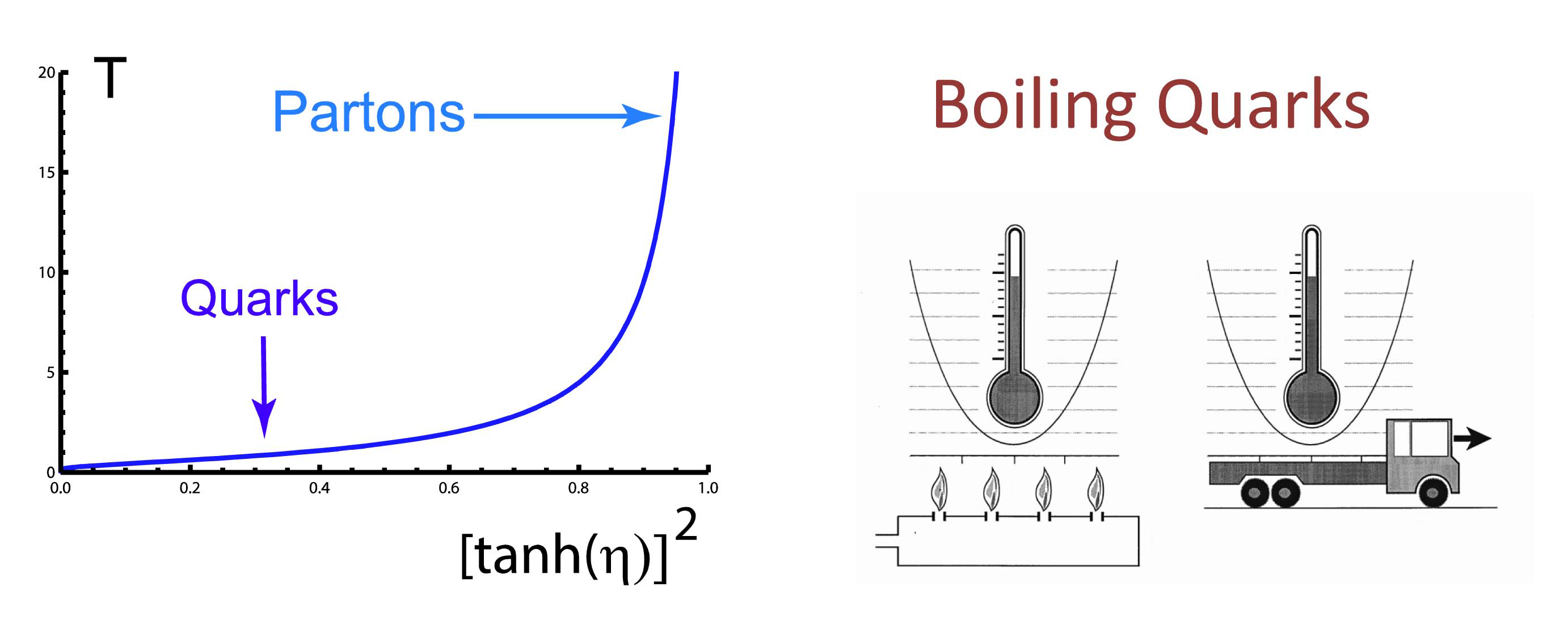
Figure 8: Boiling quarks become partons. When the hadron gains speed, the temperature of system rises according to Eq.(50). The quarks will boil, and they will go through a phase transition to partons as is indicated in Fig. 9.

Let us look at the velocity dependence of the temperature again. It is almost proportional to the velocity from $\tanh(\eta)=0$ to $0.7$, and again from $\tanh(\eta)=0.9$ to $1$ with different slopes. We shall return to this issue in Sec. 5 in connection with the transition from the quark model to the parton model.

While the physical motivation for this section was based on Feynman’s time separation variable [9] and his rest of the universe [23], we should note that many authors discussed field theoretic approach to derive the density matrix of Eq.(47). Among them are two-mode squeezed states of light [14, 15, 16, 17] and thermo-field-dynamics [33, 34, 35].

The mathematics of two-mode squeezed states is the same as that for the covariant harmonic oscillator formalism discussed in this paper [4, 15, 16, 17]. Instead of the $z$ and $t$ coordinates, there are two measurable photons. If we choose not to observe one of them, it belongs to Feynman’s rest of the universe [21, 36, 37].

Another remarkable feature of two-mode squeezed states of light is that its formalism is identical to that of thermo-field-dynamics [33, 38, 34, 35]. The temperature is in this case related to the squeeze parameter. It is therefore possible to define the temperature of a Lorentz-squeezed hadron within the framework of the covariant harmonic oscillator model.

5 Quark-Parton Phase Transitions

Let us go back to Fig.(8). There the hadronic temperature $T$ is plotted against $\tanh^{2}(\eta)$ or $(v/c)^{2}$. We can also plot $(v/c)^{2}$ as a function of $T$, as shown in Fig. 9.

As is seen in Fig. 9, the curve is nearly vertical for low temperature, but becomes nearly horizontal for high temperature, even though it is continuous. Thus, we are led to suspect a phase transition between these two different sections of the curve. Let us look at what happened inside the hadron.

If the hadron is at rest or its speed is very low, we use the quark model. If the hadron is moving with the speed close to that of light, we use the parton model. Since the constituents behave quite differently in these two models, we are confronted with the question of whether they can be described as two different limiting cases of one covariant entity.

This kind of question is not new in physics. Before 1905, Einstein faced the question of two different energy-momentum relations for massive and massless particles. He ended up with the formula $E=\sqrt{m^{2}+p^{2}}$, which is widely known as his $E=mc^{2}$.

Our quark-parton puzzle is similar to that of energy-momentum relation, as illustrated in Table 1. The dynamics of the quark model is the same as that of the hydrogen atom, where two constituent particles are bound together by an attractive force.

We are all familiar with the dynamics of the hydrogen atom, but it is a challenge to understand Feynman’s parton picture as a Lorentz-boosted hydrogen atom. The key variable is the time-separation between the quarks, not seen in the Schrödinger picture of the hydrogen atom. This variable has been studied in detail in Sec. 3.

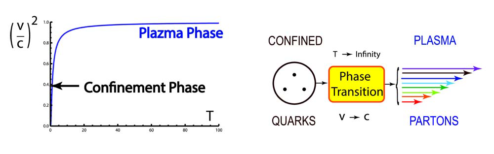
Figure 9: Transition from the confinement phase to a plasma phase. The quarks are confined within a hadron when the hadron is at rest, but they behave like free particles when the hadron speed reaches that of light, and the temperature becomes very high. This figure is a extended interpretation of Fig. 8.

Table 1: Massive and massless particles in one package. Einstein unified the energy-momentum relation for slow (massive) and fast (massless) particles with one Lorentz-covariant formula.

	Massive	Lorentz	Massless
	Slow	Covariance	Fast
Energy-	$E=$	Einstein’s
Momentum	$p^{2}/2m$	$E=[p^{2}+m^{2}]^{1/2}$	$E=p$
Hadron’s	Gell-Mann’s	Lorentz-covariant	Feynman’s
Constituents	Quark Model	Harmonic Oscillator	Parton Picture

5.1 Feynman’s Parton Picture

In a hydrogen atom or a hadron consisting of two quarks, there is a spacial separation between two constituent elements. In the case of the hydrogen atom we call it the Bohr radius. If the atom or hadron is at rest, the time-separation variable does not play any visible role in quantum mechanics. However, if the system is boosted to the Lorentz frame which moves with a speed close to that of light, this time-separation variable becomes as important as the space separation of the Bohr radius. Thus, the time-separation plays a visible role in high-energy physics which studies fast-moving bound states. Let us study this problem in more detail.

It is a widely accepted view that hadrons are quantum bound states of quarks having a localized probability distribution. As in all bound-state cases, this localization condition is responsible for the existence of discrete mass spectra. The most convincing evidence for this bound-state picture is the hadronic mass spectra [9, 6]. However, this picture of bound states is applicable only to observers in the Lorentz frame in which the hadron is at rest. How would the hadrons appear to observers in other Lorentz frames?

In 1969, Feynman observed that a fast-moving hadron can be regarded as a collection of many “partons” whose properties appear to be quite different from those of the quarks [29, 30]. For example, the number of quarks inside a static proton is three, while the number of partons in a rapidly moving proton appears to be infinite. The question then is how the proton looking like a bound state of quarks to one observer can appear different to an observer in a different Lorentz frame? Feynman made the following systematic observations.

• The picture is valid only for hadrons moving with velocity close to that of light.

• The interaction time between the quarks becomes dilated, and partons behave as free independent particles.

• The momentum distribution of partons becomes widespread as the hadron moves fast.

• The number of partons seems to be infinite or much larger than that of quarks.

Because the hadron is believed to be a bound state of two or three quarks, each of the above phenomena appears as a paradox, particularly b) and c) together. How can a free particle have a wide-spread momentum distribution?

In order to resolve this paradox, let us construct the momentum-energy wave function corresponding to the Gaussian form of Eq.(21). If the quarks have the four-momenta $p_{a}$ and $p_{b}$, we can construct two independent four-momentum variables [9]

$$P=p_{a}+p_{b},\qquad p=\sqrt{2}(p_{a}-p_{b}).$$ (51)

The four-momentum $P$ is the total four-momentum and is thus the hadronic four-momentum. $p$ measures the four-momentum separation between the quarks. Their light-cone variables are

$$p_{u}=\frac{p_{0}-p_{z}}{\sqrt{2}},\qquad p_{v}=\frac{p_{0}+p_{z}}{\sqrt{2}},$$ (52)

with the Lorentz-boost property

$$p_{u}\rightarrow e^{-\eta}p_{u}\qquad p_{v}\rightarrow e^{\eta}p_{v}.$$ (53)

The momentum-energy wave function is

$$\phi_{\eta}(p_{z},p_{0})=\frac{1}{2\pi}\int\psi_{\eta}(z,t)\exp{\left\{i\left(zp_{z}-tp_{0}\right)\right\}}dzdt$$ (54)

where $\psi_{\eta}$ is the space-time wave function of Eq.(43). The evaluation of this integral leads to

$$\phi_{\eta}(p_{z},p_{0})=\left({1\over\pi}\right)^{1/2}\exp\left\{-{1\over 2}\left[e^{-2\eta}p_{u}^{2}+e^{2\eta}p_{v}^{2}\right]\right\}.$$ (55)

Because we are using here the harmonic oscillator, the mathematical form of the above momentum-energy wave function is the same as that of the space-time wave function of Eq.(30) in its ground state.

The Lorentz squeeze properties of these wave functions are also the same, as is indicated in Fig. 2. This aspect of the squeeze has been exhaustively discussed in the literature [6, 39, 40], and they are illustrated again in Fig. 10 of the present paper. The hadronic structure function calculated from this formalism is in a reasonable agreement with the experimental data [41].

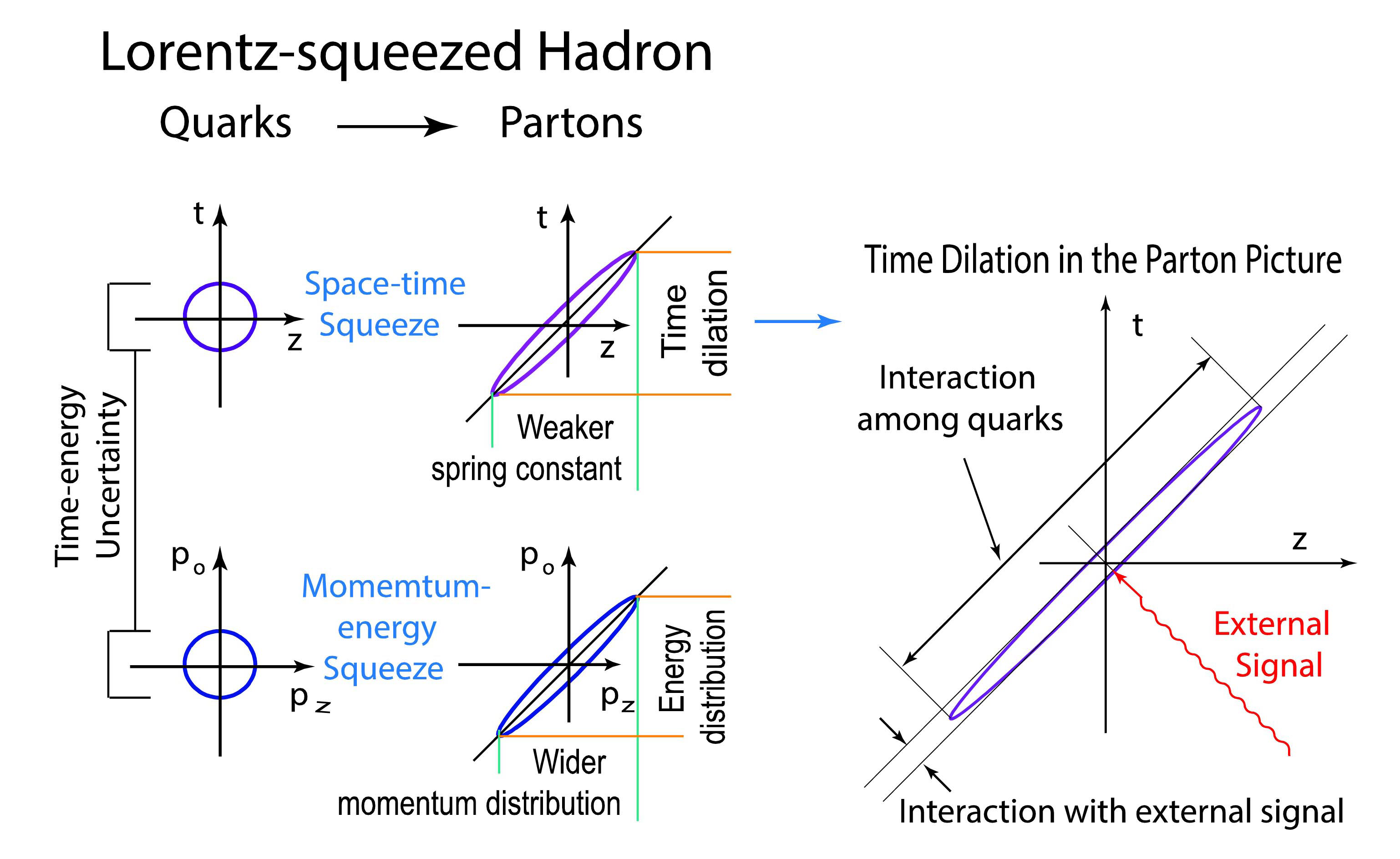
Figure 10: Lorentz-squeezed space-time and momentum-energy wave functions. As the hadron’s speed approaches that of light, both wave functions become concentrated along their respective positive light-cone axes. These light-cone concentrations lead to Feynman’s parton picture. The interaction time of the quarks among themselves becomes dilated, as the expanding major axis of space-time ellipse indicates. On the other hand, the external signal, since it is moving in the direction opposite to the direction of the hadron, travels along the negative light-cone axis. To the external signal, if it moves with velocity of light, the hadron appears very thin, and the quark’s interaction time with the external signal becomes very small. This is called Feynman’s time dilation

When the hadron is at rest with $\eta=0$, both wave functions behave like those for the static bound state of quarks. As $\eta$ increases, the wave functions become continuously squeezed until they become concentrated along their respective positive light-cone axes. Let us look at the z-axis projection of the space-time wave function. Indeed, the width of the quark distribution increases as the hadronic speed approaches that of the speed of light. The position of each quark appears widespread to the observer in the laboratory frame, and the quarks appear like free particles.

The momentum-energy wave function is just like the space-time wave function. The longitudinal momentum distribution becomes wide-spread as the hadronic speed approaches the velocity of light. This is in contradiction with our expectation from nonrelativistic quantum mechanics that the width of the momentum distribution is inversely proportional to that of the position wave function. Our expectation is that if the quarks are free, they must have a sharply defined momenta, not a wide-spread distribution.

However, according to our Lorentz-squeezed space-time and momentum-energy wave functions, the space-time width and the momentum-energy width increase in the same direction as the hadron is boosted. This is of course an effect of Lorentz covariance. This is indeed the resolution of one of the quark-parton puzzles [6, 39, 40].

5.2 Feynman’s Decoherence

Another puzzling problem in the parton picture is that partons appear as incoherent particles, while quarks are coherent when the hadron is at rest. Does this mean that the coherence is destroyed by the Lorentz boost? The answer is known to be NO [12, 42], and we would like to expand our earlier discussion on this subject.

When the hadron is boosted, the hadronic matter becomes squeezed and becomes concentrated in the elliptic region along the positive light-cone axis. The length of the major axis becomes expanded by $e^{\eta}$, and the minor axis is contracted by $e^{-\eta}$.

This means that the interaction time of the quarks among themselves become dilated. Because the wave function becomes wide-spread, the distance between one end of the harmonic oscillator well and the other end increases. This effect, first noted by Feynman [29, 30], is universally observed in high-energy hadronic experiments. The period of oscillation increases like $e^{\eta}$.

On the other hand, the external signal, since it is moving in the direction opposite to the direction of the hadron travels along the negative light-cone axis, as illustrated in Fig. 10.

If the hadron contracts along the negative light-cone axis, the interaction time decreases by $e^{-\eta}$. The ratio of the interaction time to the oscillator period becomes $e^{-2\eta}$. The energy of each proton coming out of CERN’s LHC is $4000GeV$. This leads to a ratio of $1.6\times 10^{-8}$. This is indeed a small number. The external signal is not able to sense the interaction of the quarks among themselves inside the hadron.

Indeed, Feynman’s parton picture is one concrete physical example where the decoherence effect is observed. As for the entropy, the time-separation variable belongs to the rest of the universe. Because we are not able to observe this variable, the entropy increases as the hadron is boosted to exhibit the parton effect. The decoherence is thus accompanied by an entropy increase.

Let us go back to the coupled-oscillator system. The light-cone variables in Eq.(17) correspond to the normal coordinates in the coupled-oscillator system given in Eq.(2). According to Feynman’s parton picture, the decoherence mechanism is determined by the ratio of widths of the wave function along the two normal coordinates.

This decoherence mechanism observed in Feynman’s parton picture is quite different from other decoherences discussed in the literature. It is widely understood that the word decoherence is the loss of coherence within a system. On the other hand, Feynman’s decoherence discussed in this section comes from the way the external signal interacts with the internal constituents.

5.3 Uncertainty Relations

Let us go back to Fig. 10. Both the spatial and momentum distribution become widespread as the hadron is Lorentz-boosted. Does this mean that Plank’s constant is not Lorentz invariant? The answer is No. The uncertainty relation still remains invariant. According to Eq.(55), the major axis of the space-time ellipse is conjugate to the minor axis of the momentum-ellipse. Thus the uncertainty products

$$\left<u^{2}\right>\left<p_{u}^{2}\right>=\left<v^{2}\right>\left<p_{v}^{2}\right>$$ (56)

remain invariant under the boost.

What happens when we fail to observe the time-separation coordinate? We can approach this problem using the Wigner function [43]. For the density matrix of Eq.(34), the Wigner function is

$$W_{\eta}\left(z,t,p_{z},p_{0}\right)=\frac{1}{\pi}\int\exp{\left[(i(z^{\prime}p_{z}+t^{\prime}p_{0})\right]}\rho_{\eta}(z-z^{\prime},t-t^{\prime})dz^{\prime}dt^{\prime}$$ (57)

The evaluation of this integral is straight-forward [16, 31]. For $\eta=0$, the Wigner function becomes

$$W_{0}\left(z,p_{z};t,p_{0}\right)=\left(\frac{1}{\pi}\right)^{2}\exp{\left[-\left(z^{2}+p_{z}^{2}+t^{2}+p_{0}^{2}\right)\right]}.$$ (58)

This is the Wigner function for the minimal uncertainty state without any thermal effects, or for the hadron at rest. This Gaussian form is illustrated in Fig. 11.

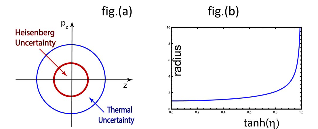
Figure 11: Uncertainty Distribution in the Wigner phase space. The radius takes the minimal value determined by the uncertainty principle when the hadron is at rest and its temperature is zero. The radius increases as the temperature rises as indicated in fig.(a). The dependence of this radius on $\tanh(\eta)$ (the hadronic speed) is also given in fig.(b).

For non-zero values of $\eta,W_{\eta}\left(z,p_{z};t,p_{0}\right)$ becomes

$$\left(\frac{1}{\pi}\right)^{2}\exp\left\{-{1\over 2}\left[e^{2\eta}(t+z)^{2}+e^{-2\eta}(t-z)^{2}+e^{-2\eta}\left(p_{z}-p_{0}\right)^{2}+e^{2\eta}\left(p_{z}+p_{0}\right)^{2}\right]\right\}.$$ (59)

If we do not observe the second pair of variables, we have to integrate this function over $t$ and $p_{0}$, and the resulting Wigner function is

$$W_{\eta}\left(z,p_{z}\right)=\int W(z,p_{z};t,p_{0})dtdp_{0},$$ (60)

and the evaluation of this integration leads to [21]

$$W_{\eta}(x,p)=\frac{1}{\pi\cosh\eta}\exp{\left[-\left(\frac{z^{2}+p_{z}^{2}}{\cosh(2\eta)}\right)\right]},$$ (61)

The failure to make measurements on the time separation variable leads to a radial expansion of the Wigner phase space as in the case of the thermal excitation. The radius is

$$\sqrt{\cosh(2\eta)}=\sqrt{\frac{1+\tanh^{2}\eta}{1-\tanh^{2}\eta}}.$$ (62)

As is indicated in Fig. 11, the radius becomes larger when $\tanh(\eta)$ becomes larger or the hadron moves with an increasing speed.

Concluding Remarks

For forty years since 1973 [44], the present authors published many papers on the subject of Lorentz-boosting standing waves. What is new in this paper?

In our first paper on this subject [44], we started with a Lorentz-covariant Gaussian form proposed by Yukawa’s in his 1953 paper [8], and its applications to high-energy physics [45, 46, 47, 48, 49]. We were particularly interested in how the Gaussian form becomes deformed under Lorentz boosts.

Since then we have been adding physical interpretations to Yukawa’s Gaussian form. In 1977 [39], using the Yukawa form, we were able to show that the quark model and the parton model are two different manifestations of the same covariant model.

In 1979, using a set of normalizable solutions of the Lorentz-invariant differential equation of Feynman [9], which includes Yukawa’s Gaussian form, we constructed representations of Wigner’s $O(3)$-like little group for massive particles [19]. Wigner’s little groups dictate the internal space-time symmetries of particles in the Lorentz-covariant world.

During the period of 1980-81, Kim and Han noted that the wave function approach starting from Yukawa is equivalent to Dirac’s plan to construct a Lorentz-covariant quantum mechanics [50, 51]. According to these papers, the covariant harmonic oscillator wave functions combine Dirac’s efforts made in his three papers [1, 2, 3] into Fig. 4.

In so doing we had to address the physics of the time separation between the two constituent particles. This variable does not exist in the Schrödinger picture of quantum mechanics, while the time-energy uncertainty relation plays the key role in calculation of transition rates [1]. The covariant harmonic oscillator embraces these two physical principles.

However, the failure to observe this time-separation variable leads to a rise in entropy and temperature. It is shown that this can be interpreted in terms of the space-time entanglement. In this paper, it was noted that the Lorentz boost entangles the longitudinal and time-like variables. We have addressed the issue of the entropy and temperature arising from this entanglement.

In Feynman’s parton picture, interaction of the quarks with the external signal should be coherent according to quantum mechanics. However, they lose coherence when they become partons. This is another physical example of decoherence.

The mathematics of the covariant harmonic oscillators is basically the same as that of the coupled harmonic oscillators. Its mathematics is transparent, and its quantum mechanics is well understood. It is gratifying to note that this simple mathematical instrument is capable of embracing many of the physical concepts developed in recent years, such as squeezed states, entanglement, decoherence, as well as the following issues raised by Feynman.

• Three-dimensional harmonic oscillators are quite adequate for describing the observed hadron spectra [9].

• We have to use harmonic oscillators, instead of Feynman diagrams, for bound-state problems in the Lorentz-covariant world. In so doing we have to deal with the problem of the time-separation variable, while Feynman did not [9].

• In 1969 [29, 30], Feynman proposed his parton model for hadrons with their speeds close to the speed of light. Since the partons appear to be quite different from ¡— the quarks inside the hadrons at rest, the question is ¡— whether Feynman’s parton model is a Lorentz-boosted quark model, or the quark and parton models are two different manifestations of one Lorentz-covariant entity. We addressed this issue in Subsec. 5.1.

• Feynman’s rest of the universe [23]. The time-separation variable exists according to Einstein. Since we are not making observations on this variable, it belongs to Feynman’s rest of the universe. We discussed in detail what happens if we do not observe this variable.

In this paper, we have addressed these Feynman issues by combining the three papers of Dirac mentioned in Sec. 3.

Finally, on the subject of combining quantum mechanics with special relativity, quantum field theory occupies an prominent place. The question then is what role QFT plays in the problems discussed in this paper. We address this issue in the Appendix.

Appendix

In this appendix, we would like discuss why we did not use the present form of quantum field theory, while it combines quantum mechanics with special relativity. Yes, quantum electrodynamics produces the Lamb shift and the correction to the electron magnetic moment. However, in order to produce the Lamb shift, we need the Rydberg formula for the hydrogen energy levels. Does the present form of QFT produce a Lorentz-covariant picture of hydrogen energy levels? The answer clearly NO. QFT does not solve all the problems.

We are not the first ones to see this difficulty. While Feynman was the person who formulated Feynman diagrams for QFT, he suggested the use of harmonic oscillators to approach tackle bound-state problems in his talk at the 1970 Washington meeting of the American physical society [9]. Since 1973 [44], we rigorously followed Feynman’s suggestion and have published a series of papers.

Feynman’s suggestion was based on the Chew-Frautschi plot of the hadronic mass spectra [52]. It was noted that they are reflections of degeneracies of the three-dimensional harmonic oscillators. Feynman et al. then wrote down a Lorentz-invariant partial differential equation for the harmonic oscillator. However, they could not produce the solution consistent with Lorentz covariance and the probability interpretation quantum mechanics.

The most serious error in this paper is their treatment of the time separation variable between the quarks. Indeed, our present paper is dedicated to a better understanding of this unobservable variable in terms of Feynman’s rest of the universe [23].

In a series of publications, we have constructed solutions of their oscillator equation consistent with Wigner’s little groups dictating internal space-time symmetries, resulting in our 1986 book [6], and consistent with Dirac’s c-number time-energy uncertainty relation [1].

The most significant result of our endeavor is to show that Gell-Mann’s quark model and Feynman’s parton model are two limiting case of one Lorentz-covariant entity. The purpose of the present paper is to elaborate on this point.

The question still is where our program stands with respect to quantum field theory. Let us go to Fig. 5. There we point out there that there are running and standing waves in quantum mechanics corresponding to scattering and bound states. They may have different forms of mathematics, but we point out they should and they do share the same set of physical principles of quantum mechanics and special relativity [18].

References

- [1] Dirac, P. A. M. The Quantum Theory of the Emission and Absorption of Radiation. Proc. Roy. Soc. (London) 1927, A114, 243-265.
- [2] Dirac, P. A. M. Unitary Representations of the Lorentz Group. Proc. Roy. Soc. (London) 1945, A183, 284-295.
- [3] Dirac, P. A. M. Forms of Relativistic Dynamics. Rev. Mod. Phys. 1949, 21, 392-399.
- [4] Dirac, P. A. M. A Remarkable Representation of the 3 + 2 de Sitter Group. J. Math. Phys. 1963, 4, 901-909.
- [5] Wigner, E. On Unitary Representations of the Inhomogeneous Lorentz Group. Ann. Math. 1939, 40, 149-204.
- [6] Y. S. Kim and M. E. Noz, Theory and Applications of the Poincaré Group (Reidel, Dordrecht, 1986).
- [7] J. S. Bell, Speakable and Unspeakable in Quantum Mechanics: Collected Papers on Quantum Philosophy, 2nd Ed. (Cambridge University Press, London, 2004). page 71. The first edition was published in 1988.
- [8] Yukawa, H. Structure and Mass Spectrum of Elementary Particles. I. General Considerations. Phys. Rev. 1953, 91, 415-416.
- [9] Feynman, R. P.; Kislinger, M.; Ravndal F.; Current Matrix Elements from a Relativistic Quark Model. Phys. Rev. D 1971, 3, 2706-2732.
- [10] Kim, Y. S.; Noz, M. E.; Oh, S. H.; A Simple Method for Illustrating the Difference between the Homogeneous and Inhomogeneous Lorentz Groups. Am. J. Phys. 1979, 47, 892-897.
- [11] Giedke G., Wolf M. M., Krüger O, Werner R. F, and J. L. Cirac J. L. 2003 Phys. Rev. Lett. 1003, 91, 107901.
- [12] Kim, Y. S.; Noz, M. E.; Coupled oscillators, entangled oscillators, and Lorentz-covariant harmonic oscillators. J. Opt. B: Quantum and Semiclass. Opt. 2005, 7, S458-S467.
- [13] Kim, Y. S.; Noz, M. E. Lorentz Harmonics, Squeeze Harmonics and Their Physical Applications. Symmetry 2011, 3, 16-36.
- [14] Yuen, H. P.; Two-photon coherent states of the radiation field. Phys. Rev. A 1976, 13, 2226-2243.
- [15] Yurke, B. S.; L. McCall, B. L.; Klauder, J. R.; SU(2) and SU(1,1) interferometers. Phys. Rev. A 1986, 33, 4033-4054.
- [16] Kim, Y. S.; Noz, M. E. Phase Space Picture of Quantum Mechanics. World Scientific Publishing Company, Singapore 1991.
- [17] Han, D.; Kim, Y.S.; Noz, M. E.; Yeh, L.; Symmetries of Two-mode Squeezed States. J. Math. Phys. 1993, 34, 5493-5508.
- [18] Han,D,; Kim, Y. S.; Noz, M. E. Physical Principles in Quantum Field Theory and Covariant Harmonic Oscillators. Found. of Phys. 1081 11, 895-903.
- [19] Kim, Y. S.; Noz, M. E.; Oh, S. H. Representations of the Poincaré group for relativistic extended hadrons. J. Math. Phys. 1979, 20, 1341-1344.
- [20] Ruiz, M. J. Orthogonality relations for covariant harmonic oscillator wave functions. Phys. Rev. D 1974, 10, 4306-4307.
- [21] Han, D.; Kim, Y. S.; Noz, M. E. Illustrative Example of Feynman’s Rest of the Universe. Am. J. Phys. 1999, 67, 61-66.
- [22] Kim, Y. S.; Wigner, E. P. Entropy and Lorentz Transformations. Phys. Lett. A 1990, 147, 343-347.
- [23] Feynman, R. P. Statistical Mechanics. Benjamin/Cummings: Reading, MA 1972.
- [24] von Neumann, J. Die mathematische Grundlagen der Quanten-mechanik. Springer: Berlin, 1932.
- [25] Fano, U. Description of States in Quantum Mechanics by Density Matrix and Operator Techniques. Rev. Mod. Phys. 1967, 29, 74-93.
- [26] Landau, L. D.; Lifshitz, E. M.; Statistical Physics. Pergamon Press, London 1958.
- [27] Wigner E. P,; Yanase, M. M. Information Contents of Distributions. Proc. National Academy of Sciences (U.S.A.) 1963, 49, 910-918.
- [28] Kim, Y. S.; Li, M.; Squeezed States and Thermally Excited States in the Wigner Phase-Space Picture of Quantum Mechanics. Phys. Lett. A 1989, 139, 445-448.
- [29] Feynman, R. P. Very High-Energy Collisions of Hadrons. Phys. Rev. Lett. 1969, 23, 1415-1417.
- [30] Feynman, R. P. The Behavior of Hadron Collisions at Extreme Energies in High-Energy Collisions. In Proceedings of the Third International Conference, Stony Brook, NY (Yang, C. N.; et al. Eds.), Gordon and Breach: New York 1969, pp 237-249.
- [31] Davies, R. W.; Davies, K. T. R. On the Wigner distribution function for an oscillator. Ann. Phys. 1975, 89, 261-273.
- [32] Han, D.; Kim, Y. S.; Noz, M. E. Lorentz-Squeezed Hadrons and Hadronic Temperature. Phys. Lett. A 1990, 144, 111-115.
- [33] Fetter, A. L.; Walecka, J. D. Quantum Theory of Many-Particle Systems. McGraw-Hill, New York 1971.
- [34] Umezawa, H.; Matsumoto, H; Tachiki, M. Thermo Field Dynamics and Condensed States. North-Holland, Amsterdam 1982.
-
[35]
Mann; A.; Revzen, M. Thermal coherent states. Phys. Lett. A
1989, 134, 273-275.
A. Kireev1, A.; A. Mann, A.; Revzen, M., Umezawa, H. Thermal squeezed states in thermo field dynamics and quantum and thermal fluctuations. Phys. Lett. A 1989, 142, 215-221.
Oz-Vogta, J.; Manna, A; Revzen, M. Thermal Coherent States and Thermal Squeezed States. J. Mod. Optics 1991, 38, 2339-2347. - [36] Yurke, B; Potasek, M. Obtainment of Thermal Noise from a Pure State. Phys. Rev. A 1987, 36, 3464-3466.
- [37] Ekert, A. K.; Knight, P. L. Correlations and squeezing of two-mode oscillations. Am. J. Phys. 1989, 57, 692-697.
- [38] Ojima, I. Gauge Fields at Finite Temperatures-“Therm0 Field Dynamics” and the KMS Condition and Their Extension to Gauge Theories. Ann. Phys. (NY), 1981, 137 1-32.
- [39] Kim, Y. S.; Noz, M. E. Covariant Harmonic Oscillators and the Parton Picture. Phys. Rev. D 1977, 15, 335-338.
- [40] Kim, Y. S. Observable gauge transformations in the parton picture. Phys. Rev. Lett. 1989, 63, 348-351.
- [41] Hussar, P. E. Valons and harmonic oscillators. Phys. Rev. D 1981, 23, 2781-2783.
- [42] Kim, Y. S.; Noz, M. E. Feynman’s Decoherence. Optics and Spectro. 2003 47, 733-740.
- [43] Wigner, E. On the Quantum Corrections for Thermodynamic Equilibrium. Phys. Rev. 1932, 40, 749-759 (1932).
- [44] Kim, Y. S.; Noz, M. E. Covariant harmonic oscillators and the quark model. Phys. Rev. D 1973, 8, 3521-3627.
- [45] Markov, M. On Dynamically Deformable Form Factors in the Theory of Particles. Suppl. Nuovo Cimento 1956, 3, 760-772.
- [46] Ginzburg, V. L.; Man’ko, V. I. Relativistic oscillator models of elementary particles. Nucl. Phys. 1965, 74, 577-588.
- [47] Fujimura, K.; Kobayashi, T.; Namiki, M. Nucleon Electromagnetic Form Factors at High Momentum Transfers in an Extended Particle Model Based on the Quark Model. Prog. Theor. Phys. 1970, 43, 73-79.
- [48] Licht, A. L.; Pagnamenta, A. Wave Functions and Form Factors for Relativistic Composite Particles I. Phys. Rev. D 1970, 2, 1150-1156.
- [49] Lipes, R. Electromagnetic Excitations of the Nucleon in a Relativistic Quark Model. Phys Rev. D 1972, 5, 2849-2863.
- [50] Han, D.; Kim, Y. S. Yukawa’s Approach and Dirac’s Approach to Relativistic Quantum Mechanics. Prog. Theor. Phys. 1980, 64, 1852-1860.
- [51] Han, D.; Kim, Y. S. Dirac’s Form of Relativistic Quantum Mechanics. Am. J. Phys. 1981, 49, 1157-1161.
- [52] Chew, G. F. S-Matrix Theory of Strong Interactions without Elementary Particles Rev. Mod. Phys. 1962, 34, 394 400.