Convergence of adaptive BEM and adaptive FEM-BEM coupling for estimators without $h$-weighting factor

Abstract.

We analyze adaptive mesh-refining algorithms in the frame of boundary element methods (BEM) and the coupling of finite elements and boundary elements (FEM-BEM). Adaptivity is driven by the two-level error estimator proposed by Ernst P. Stephan, Norbert Heuer, and coworkers in the frame of BEM and FEM-BEM or by the residual error estimator introduced by Birgit Faermann for BEM for weakly-singular integral equations. We prove that in either case the usual adaptive algorithm drives the associated error estimator to zero. Emphasis is put on the fact that the error estimators considered are not even globally equivalent to weighted-residual error estimators for which recently convergence with quasi-optimal algebraic rates has been derived.

1. Introduction

A posteriori error estimation and related adaptive mesh-refining algorithms are one important basement of modern scientific computing. Starting from an initial mesh ${\mathcal{T}}_{0}$ and based on a computable a posteriori error estimator, such algorithms iterate the loop

$$\boxed{\texttt{~{}solve~{}}}\quad\to\quad\boxed{\texttt{~{}estimate~{}}}\quad\to\quad\boxed{\texttt{~{}mark~{}}}\quad\to\quad\boxed{\texttt{~{}refine~{}}}$$ (1)

to create a sequence of successive locally refined meshes ${\mathcal{T}}_{\ell}$, corresponding discrete solutions $U_{\ell}$, as well as a posteriori error estimators $\mu_{\ell}$. We consider the frame of conforming Galerkin discretizations, where ${\mathcal{T}}_{\ell}$ is linked to a finite-dimensional subspace ${\mathcal{X}}_{\ell}$ of a Hilbert space ${\mathcal{H}}$ with corresponding Galerkin solution $U_{\ell}\in{\mathcal{X}}_{\ell}$, where successive refinement guarantees nestedness ${\mathcal{X}}_{\ell}\subseteq{\mathcal{X}}_{\ell+1}\subset{\mathcal{H}}$ for all $\ell\in{\mathbb{N}}_{0}$.

Convergence of this type of adaptive algorithm in the sense of

$$\lim_{\ell\to\infty}\|u-U_{\ell}\|_{{\mathcal{H}}}=0$$ (2)

has first been addressed in [BV84] for 1D FEM and [Dör96] for 2D FEM. We note that already the pioneering work [BV84] observed that validity of some Céa-type quasi-optimality and nestedness ${\mathcal{X}}_{\ell}\subseteq{\mathcal{X}}_{\ell+1}$ for all $\ell\in{\mathbb{N}}_{0}$ imply a priori convergence

$$\lim_{\ell\to\infty}\|U_{\infty}-U_{\ell}\|_{{\mathcal{H}}}=0,$$ (3)

where $U_{\infty}$ is the unique Galerkin solution in ${\mathcal{X}}_{\infty}:=\overline{\bigcup_{\ell\in{\mathbb{N}}_{0}}{\mathcal{X}}_{\ell}}$. From a conceptual point of view, it thus only remained to identify the limit $u=U_{\infty}$. Based on such an a priori convergence result (3), a general theory of convergence of adaptive FEM is devised in [MSV08, Sie11], where the analytical focus is on estimator convergence

$$\lim_{\ell\to\infty}\mu_{\ell}=0.$$ (4)

Moreover, the recent work [CFPP14] gives an analytical frame to guarantee convergence with optimal convergence rates; see also the overview article [FFH⁺14] for the current state of the art of adaptive BEM. Throughout, it is however implicitly assumed that the local contributions $\mu_{\ell}(T)$ of the error estimator $\mu_{\ell}$ are weighted with the local mesh-size, i.e., $|T|^{\alpha}$ for some appropriate $\alpha>0$, or that $\mu_{\ell}$ is locally equivalent to a mesh-size weighted error estimator.

In this work, we consider two particular error estimators whose local contributions are not weighted by the local mesh-size. We devise a joint analytical frame which proves estimator convergence (4). First, we let $\mu_{\ell}$ be the Faermann error estimator [Fae00, Fae02, CF01] for BEM for the weakly-singular integral equation with ${\mathcal{H}}=\widetilde{H}^{-1/2}(\Gamma)$. The local contributions of $\mu_{\ell}$ are overlapping $H^{1/2}$-seminorms of the residual $F-AU_{\ell}\in H^{1/2}(\Gamma)$. The striking point of $\mu_{\ell}$ is that it is the only a posteriori BEM error estimator which is known to be both reliable and efficient without any further assumptions on the given data, i.e., it holds

$$C_{\rm eff}^{-1}\,\mu_{\ell}\leq\|u-U_{\ell}\|_{{\mathcal{H}}}\leq C_{\rm rel}\,\mu_{\ell}$$ (5)

with $\ell$-independent constants $C_{\rm eff},C_{\rm rel}>0$. We note that $\mu_{\ell}$ is not equivalent to an $h$-weighted error estimator which prevents to follow the arguments from the available literature.

Second, our analysis covers the two-level error estimators for BEM [MSW98, MMS97, MS00, HMS01, Heu02, EH06] or the adaptive FEM-BEM coupling [MS99, KMS10, GMS12, AFKP12]. The local contributions are projections of the computable error between two Galerkin solutions onto one-dimensional spaces, spanned by hierarchical basis functions. These estimators are known to be efficient. On the other hand, reliability is only proven under an appropriate saturation assumption which is even equivalent to reliability for the symmetric BEM operators [EFLFP09, EFGP13, AFF⁺14]. However, such a saturation assumption is formally equivalent to asymptotic convergence of the adaptive algorithm [FLP08] which cannot be guaranteed mathematically in general and is expected to fail on coarse meshes.

Outline. The remainder of the paper is organized as follows: In Section 2, we introduce an abstract frame which covers both BEM as well as the FEM-BEM coupling. We formally state the adaptive loop (Algorithm 2). Under three assumptions on the error estimator which are later verified for the particular model problems, we prove that the adaptive loop drives the underlying error estimator to zero (Proposition 4 and Proposition 5). Section 3 treats the weakly-singular integral equation associated with the Laplacian. We prove that two-level error estimator (Theorem 6) as well as Faermann error estimator (Theorem 7) fit into the abstract framework. In Section 4, we consider the hyper-singular integral equation associated with the Laplacian. We prove that the two-level error estimator fits into the abstract framework (Theorem 11). The final Section 5 considers a nonlinear Laplace transmission problem which is reformulated by some FEM-BEM coupling. We prove that the two-level error estimator fits into the abstract framework as well (Theorem 13).

Notation. Associated quantities are linked through the same index, i.e., $U_{\star}$ is the discrete solution with respect to the discrete space ${\mathcal{X}}_{\star}$ which corresponds to the triangulation ${\mathcal{T}}_{\star}$. Throughout, the star is understood as general index and may be accordingly replaced by the level of the adaptive algorithm (e.g., $U_{\ell}$) or by the infinity symbol (e.g., ${\mathcal{X}}_{\infty}$). All constants as well as their dependencies are explicitly given in statements and results. In proofs, we shall use $A\lesssim B$ to abbreviate $A\leq c\,B$ with some generic multiplicative constant $c>0$ which is clear from the context. Moreover, $A\simeq B$ abbreviates $A\lesssim B\lesssim A$.

2. Abstract setting

2.1. Model problem

Let ${\mathcal{H}}$ be a Hilbert space with dual space ${\mathcal{H}}^{*}$ and $A:{\mathcal{H}}\to{\mathcal{H}}^{*}$ be a bi-Lipschitz continuous operator, i.e.,

$$C_{\rm cont}^{-1}\,\|w-v\|_{{\mathcal{H}}}\leq\|Aw-Av\|_{{\mathcal{H}}^{*}}\leq C_{\rm cont}\,\|w-v\|_{{\mathcal{H}}}$$ (6)

for all $v,w\in{\mathcal{H}}$. Here, $\|\cdot\|_{{\mathcal{H}}^{*}}$ denotes the operator norm on ${\mathcal{H}}^{*}$,

$$\|F\|_{{\mathcal{H}}^{*}}~=\sup_{v\in{\mathcal{H}}\backslash\{0\}}\frac{|\langle F\,,\,v\rangle|}{\|v\|_{{\mathcal{H}}}}\quad\text{for all }F\in{\mathcal{H}}^{*}.$$ (7)

Suppose that there exists some subspace ${\mathcal{X}}_{00}\subseteq{\mathcal{H}}$ such that for any given closed subspace ${\mathcal{X}}_{00}\subseteq{\mathcal{X}}_{\star}\subseteq{\mathcal{H}}$ and any continuous linear functional $F\in{\mathcal{H}}^{*}$ on ${\mathcal{H}}$, the Galerkin formulation

$$\langle AU_{\star}\,,\,V_{\star}\rangle=\langle F\,,\,V_{\star}\rangle\quad\text{for all }V_{\star}\in{\mathcal{X}}_{\star}$$ (8)

admits a unique solution $U_{\star}\in{\mathcal{X}}_{\star}$, where $\langle\cdot\,,\,\cdot\rangle$ denotes the duality bracket between ${\mathcal{H}}$ and its dual ${\mathcal{H}}^{*}$. Particularly, this implies the existence of a unique solution $u\in{\mathcal{H}}$ of

$$Au=F.$$ (9)

Moreover, we suppose that there holds the Céa-type estimate

$$\|u-U_{\star}\|_{{\mathcal{H}}}\leq C_{\mbox{\rm\scriptsize C\'{e}a}}\,\min_{V_{\star}\in{\mathcal{X}}_{\star}}\|u-V_{\star}\|_{{\mathcal{H}}},$$ (10)

where the constant $C_{\mbox{\rm\scriptsize C\'{e}a}}>0$ depends only on the operator $A$ (and possibly on $F$). To be precise, we will write $u=u(F)$ and $U_{\star}=U_{\star}(F)$ in the following to indicate that $u(F)$ resp. $U_{\star}(F)$ are the unique solutions with respect to some given right-hand side $F\in{\mathcal{H}}^{*}$.

Remark 1.  (i) The assumptions (6)–(10) are particularly satisfied with ${\mathcal{X}}_{00}=\{0\}$, $C_{\rm cont}=\max\{\widetilde{C}_{\rm cont},C_{\rm mon}^{-1}\}$, and $C_{\mbox{\rm\scriptsize C\'{e}a}}=\widetilde{C}_{\rm cont}/C_{\rm mon}$ if $A$ is Lipschitz continuous and strongly monotone in the sense

$$\|Aw-Av\|_{{\mathcal{H}}^{*}}\leq\widetilde{C}_{\rm cont}\,\|w-v\|_{{\mathcal{H}}}\quad\text{and}\quad C_{\rm mon}\|w-v\|_{{\mathcal{H}}}^{2}\leq\langle Aw-Av\,,\,w-v\rangle$$ (11)

for all $v,w\in{\mathcal{H}}$; see e.g. [Zei90, Section 25.4] for the corresponding proofs. In particular, this also covers linear problems in the frame of the Lax-Milgram lemma, e.g., the symmetric BEM formulations of Section 3–4.

(ii) The assumptions (6)–(10) are motivated by the FEM-BEM coupling formulations in Section 5.

(iii) For $A$ being linear, it is also sufficient if additionally to (6), $A$ satisfies a uniform inf-sup-condition along the sequence of discrete subspaces ${\mathcal{X}}_{\ell}$ generated by Algorithm 2 below. ∎

2.2. Adaptive algorithm

We shall assume that ${\mathcal{X}}_{\ell}$ is a finite-dimensional subspace of ${\mathcal{H}}$ related to some triangulation ${\mathcal{T}}_{\ell}$ and that $U_{\ell}(F)\in{\mathcal{X}}_{\ell}$ is the corresponding Galerkin solution (8) for ${\mathcal{X}}_{\star}={\mathcal{X}}_{\ell}$. Starting from an initial mesh ${\mathcal{T}}_{0}$, the triangulations ${\mathcal{T}}_{\ell}$ are successively refined by means of the following realization of (1), where

$$\mu_{\ell}(F):=\mu_{\ell}(F;{\mathcal{T}}_{\ell})\quad\text{with}\quad\mu_{\ell}(F;{\mathcal{E}}_{\ell}):=\Big{(}\sum_{T\in{\mathcal{E}}_{\ell}}\mu_{\ell}(F;T)^{2}\Big{)}^{1/2}<\infty\quad\text{for all }{\mathcal{E}}_{\ell}\subseteq{\mathcal{T}}_{\ell}$$ (12)

is a computable a posteriori error estimator. Its local contributions $\mu_{\ell}(F;T)\geq 0$ measure, at least heuristically, the error $u(F)-U_{\ell}(F)$ locally on each element $T\in{\mathcal{T}}_{\ell}$.

Algorithm 2.

Input: Right-hand side $F\in{\mathcal{H}}^{*}$, initial mesh ${\mathcal{T}}_{0}$ with ${\mathcal{X}}_{0}\supseteq{\mathcal{X}}_{00}$, and bulk parameter $0<\theta\leq 1$.
For $\ell=0,1,2,\dots$ iterate the following:

• Compute Galerkin solution $U_{\ell}(F)\in{\mathcal{X}}_{\ell}$.

• Compute refinement indicators $\mu_{\ell}(F;T)$ for all $T\in{\mathcal{T}}_{\ell}$.

• Determine some set ${\mathcal{M}}_{\ell}\subseteq{\mathcal{T}}_{\ell}$ of marked elements which satisfies

  $$\theta\,\mu_{\ell}(F)^{2}\leq\mu_{\ell}(F;{\mathcal{M}}_{\ell})^{2}.$$ (13)

• Generate a new mesh ${\mathcal{T}}_{\ell+1}$ and hence an enriched space ${\mathcal{X}}_{\ell+1}$ by refinement of at least all marked elements $T\in{\mathcal{M}}_{\ell}$.

Output: Sequence of successively refined triangulations ${\mathcal{T}}_{\ell}$ as well as corresponding Galerkin solutions $U_{\ell}(F)\in{\mathcal{X}}_{\ell}$ and error estimators $\mu_{\ell}(F)$, for $\ell\in{\mathbb{N}}_{0}$.

2.3. Auxiliary estimator and assumptions

The following convergence results of Proposition 4 and Proposition 5 require an auxiliary error estimator

$$\rho_{\ell}(F):=\rho_{\ell}(F;{\mathcal{T}}_{\ell})\quad\text{with}\quad\rho_{\ell}(F;{\mathcal{E}}_{\ell}):=\Big{(}\sum_{T\in{\mathcal{E}}_{\ell}}\rho_{\ell}(F;T)^{2}\Big{)}^{1/2}<\infty\quad\text{for all }{\mathcal{E}}_{\ell}\subseteq{\mathcal{T}}_{\ell}$$ (14)

with local contributions $\rho_{\ell}(F;T)\geq 0$. For all $\ell\in{\mathbb{N}}_{0}$, we suppose that there exists some superset ${\mathcal{M}}_{\ell}\subseteq{\mathcal{R}}_{\ell}\subseteq{\mathcal{T}}_{\ell}$ which satisfies the following three assumptions (A1)–(A3):

1. $\mu_{\ell}(F)$ is a local lower bound of $\rho_{\ell}(F)$: There is a constant $C_{\ref{constlocal}}>0$ such that for all $\ell\in{\mathbb{N}}_{0}$ holds

   $$\mu_{\ell}(F;{\mathcal{M}}_{\ell})\leq C_{\ref{constlocal}}\,\rho_{\ell}(F;{\mathcal{R}}_{\ell}).$$ (15)

2. $\rho_{\ell}(F)$ is contractive on ${\mathcal{R}}_{\ell}$: There is a constant $C_{\ref{constinv}}>0$ such that for all $\ell,k\in{\mathbb{N}}_{0}$ and all $\delta>0$ holds

   $$C_{\ref{constinv}}^{-1}\,\rho_{\ell}(F;{\mathcal{R}}_{\ell})^{2}\leq\rho_{\ell}(F)^{2}-\frac{1}{1+\delta}\,\rho_{\ell+k}(F)^{2}+(1+\delta^{-1})C_{\ref{constinv}}\,\|U_{\ell+k}(F)-U_{\ell}(F)\|_{{\mathcal{H}}}^{2}.$$ (16)

The constants $C_{\ref{constlocal}},C_{\ref{constinv}}>0$ may depend on $F$, but are independent of the step $\ell\in{\mathbb{N}}_{0}$, i.e., in particular independent of the discrete spaces ${\mathcal{X}}_{\ell}$ and the corresponding Galerkin solutions $U_{\ell}(F)$. If $\rho_{\ell}(F)$ is not well-defined for all $F\in{\mathcal{H}}^{*}$, but only on a dense subset $D\subseteq{\mathcal{H}}^{*}$, we require the following additional assumption:

1. $\mu_{\ell}(\cdot)$ is stable on ${\mathcal{M}}_{\ell}$ with respect to $F$: There is a constant $C_{\ref{conststable}}>0$ such that for all $\ell\in{\mathbb{N}}_{0}$ and $F^{\prime}\in{\mathcal{H}}^{*}$ holds

   $$|\mu_{\ell}(F;{\mathcal{M}}_{\ell})-\mu_{\ell}(F^{\prime};{\mathcal{M}}_{\ell})|\leq C_{\ref{conststable}}\|F-F^{\prime}\|_{{\mathcal{H}}^{*}}.$$ (17)

2.4. Remarks

Some remarks are in order to relate the abstract assumptions (A1)–(A3) to the applications, we have in mind.

$\bullet$ Choice of $\boldsymbol{\rho_{\ell}}$. Below, we shall verify that assumptions (A1)–(A3) hold with $\mu_{\ell}(F)$ being the Faermann error estimator [Fae00, Fae02, CF01] for BEM resp. $\mu_{\ell}(F)$ being the two-level error estimator for BEM [MSW98, MMS97, MS00, HMS01, Heu02, EH06, EFLFP09, EFGP13, AFF⁺14] and the FEM-BEM coupling [MS99, GMS12, AFKP12]. In either case, $\rho_{\ell}(F)$ denotes some weighted-residual error estimator, see [CS95b, CS96, Car97, CMS01, CMPS04] for BEM and [CS95a, GMS12, AFF⁺13a] for the FEM-BEM coupling.

$\bullet$ Necessity of (A3). In these cases, the weighted-residual error estimator $\rho_{\ell}$ imposes additional regularity assumptions on the given right-hand side $F$. For instance, the weighted-residual error estimator for the weakly-singular integral equation [CS95b, CS96, Car97, CMS01] requires $F\in H^{1}(\Gamma)$, while the natural space for the residual is $H^{1/2}(\Gamma)$, see Section 3 for further details and discussions. Convergence (4) of Algorithm 2 for arbitrary $F\in H^{1/2}(\Gamma)$ then follows by means of stability (A3).

$\bullet$ Verification of (A1)–(A2). For two-level estimators, (A1) has first been observed in [CF01, CMPS04] for BEM and [AFKP12] for the FEM-BEM coupling and follows essentially from scaling arguments for the hierarchical basis functions. For the Faermann error estimator and a simplified 2D BEM setting, (A1) is also proved in [CF01]. Finally, the novel observation (A2) follows from an appropriately constructed mesh-size function and refinement of marked elements as well as appropriate inverse-type estimates, where we shall build on the recent developments of [AFF⁺12]; see e.g. the proof of Theorem 6.

$\bullet$ Verification of (A3). Suppose that the operator $A$ is linear and $\mu_{\ell}(\cdot)$ is efficient

$$\mu_{\ell}(F)\leq C_{\rm eff}\,\|u(F)-U_{\ell}(F)\|_{{\mathcal{H}}}\quad\text{for all }F\in{\mathcal{H}}^{*}.$$ (18)

Provided $\mu_{\ell}(\cdot)$ has a semi-norm structure, the corresponding triangle inequality yields

$$\begin{split}\mu_{\ell}(F)\leq\mu_{\ell}(F^{\prime})+\mu_{\ell}(F-F^{\prime})&\leq\mu_{\ell}(F^{\prime})+C_{\rm eff}\,\|u(F-F^{\prime})-U_{\ell}(F-F^{\prime})\|_{{\mathcal{H}}}\\ &\leq\mu_{\ell}(F^{\prime})+C_{\rm eff}C_{\mbox{\rm\scriptsize C\'{e}a}}\,\|u(F-F^{\prime})\|_{{\mathcal{H}}}\\ &\leq\mu_{\ell}(F^{\prime})+C_{\rm eff}C_{\mbox{\rm\scriptsize C\'{e}a}}\,\|A^{-1}\|\,\|F-F^{\prime}\|_{{\mathcal{H}}^{*}},\end{split}$$ (19)

where $\|A^{-1}\|$ denotes the operator norm of $A^{-1}$, and the (bounded) inverse exists due to (6). This proves stability (A3) with $C_{\ref{conststable}}=C_{\rm eff}C_{\mbox{\rm\scriptsize C\'{e}a}}\,\|A^{-1}\|$.

$\bullet$ Marking strategy. In view of optimal convergence rates, one usually asks for $\#{\mathcal{R}}_{\ell}\lesssim\#{\mathcal{M}}_{\ell}$ in (A1) and minimal cardinality of ${\mathcal{M}}_{\ell}$ in (13). We stress, however, that this is not necessary for the present analysis, where our focus is on a first plain convergence result.

2.5. Abstract convergence analysis

We start with the observation that (A2) already implies convergence of the auxiliary estimator $\rho_{\ell}$. We note that the following lemma is, in particular, independent of the marking strategy (13), i.e., we do not use any information about how the sequence $({\mathcal{T}}_{\ell})_{\ell\in{\mathbb{N}}_{0}}$ is generated.

Lemma 3.

Suppose (A2) for some fixed $F\in{\mathcal{H}}^{*}$. Under nestedness ${\mathcal{X}}_{\ell}\subseteq{\mathcal{X}}_{\ell+1}$ of the discrete spaces for all $\ell\in{\mathbb{N}}_{0}$, the auxiliary estimator $\rho_{\ell}(F)$ converges, i.e, the limit

$$\rho_{\infty}(F):=\lim_{\ell\to\infty}\rho_{\ell}(F)$$ (20)

exists in ${\mathbb{R}}$. Moreover, it holds

$$\lim_{\ell\to\infty}\rho_{\ell}(F;{\mathcal{R}}_{\ell})=0.$$ (21)

Proof.

First, we prove that (A2) implies boundedness of $(\rho_{\ell})_{\ell\in{\mathbb{N}}_{0}}$. We recall that nestedness ${\mathcal{X}}_{\ell}\subseteq{\mathcal{X}}_{\ell+1}$ for all $\ell\in{\mathbb{N}}_{0}$ in combination with the Céa lemma (10) implies that the limit $\lim_{\ell}U_{\ell}(F)=:U_{\infty}(F)$ exists in ${\mathcal{H}}$, see e.g. [MSV08, CP12, AFLP12] or even the pioneering work [BV84]. For $\ell=0$ and $\delta=1$, assumption (A2) implies

$$\frac{1}{2}\,\rho_{k}(F)^{2}\leq\rho_{0}(F)^{2}+2C_{\ref{constinv}}\,\sup_{k\in{\mathbb{N}}_{0}}\|U_{0}-U_{k}\|_{{\mathcal{H}}}^{2}\leq M<\infty.$$

Next, we multiply  (A2) by $(1+\delta)$ and observe

$$0\leq\rho_{\ell}(F;{\mathcal{R}}_{\ell})^{2}\lesssim\rho_{\ell}(F)^{2}-\rho_{\ell+k}(F)^{2}+\delta\rho_{\ell}(F)^{2}+C_{\ref{constinv}}(\delta)\|U_{\ell+k}(F)\!-\!U_{\ell}(F)\|_{{\mathcal{H}}}^{2}$$ (22)

with $C_{\ref{constinv}}(\delta):=(1+\delta)(1+\delta^{-1})C_{\ref{constinv}}=\delta^{-1}(1+\delta)^{2}C_{\ref{constinv}}$. Let $\varepsilon>0$. Because of the boundedness of $\rho_{\ell}(F)$, we can hence choose $\delta>0$ and $\ell_{0}\in{\mathbb{N}}$ such that

$$\delta\rho_{\ell}(F)^{2}+C_{\ref{constinv}}(\delta)\,\|U_{\ell+k}(F)-U_{\ell}(F)\|_{{\mathcal{H}}}^{2}\leq\varepsilon$$

for all $\ell\geq\ell_{0}$ and $k\in{\mathbb{N}}_{0}$. Together with (22), this shows

$$\rho_{\ell}(F)^{2}-\rho_{\ell+k}(F)^{2}\geq-\varepsilon.$$ (23)

Let $a,b\in{\mathbb{R}}$ be accumulation points of $(\rho_{\ell}(F)^{2})_{\ell\in{\mathbb{N}}_{0}}$. First, choose $\ell\geq\ell_{0}$ and $k\in{\mathbb{N}}$ such that $|\rho_{\ell}(F)^{2}-a|+|\rho_{\ell+k}(F)^{2}-b|\leq\varepsilon$. With (23), this implies

$$a-b\geq-3\varepsilon.$$

Second, choose $\ell\geq\ell_{0}$ and $k\in{\mathbb{N}}$ such that $|\rho_{\ell}(F)^{2}-b|+|\rho_{\ell+k}(F)^{2}-a|\leq\varepsilon$ to derive

$$b-a\geq-3\varepsilon.$$

Since $\varepsilon>0$ was arbitrary, the last two estimates imply $a=b$. Altogether, $(\rho_{\ell}(F)^{2})_{\ell\in{\mathbb{N}}_{0}}$ is a bounded sequence in ${\mathbb{R}}$ with unique accumulation point. By elementary calculus, $(\rho_{\ell}(F)^{2})_{\ell\in{\mathbb{N}}_{0}}$ is convergent with limit $\rho_{\infty}(F)^{2}$. Continuity of the square root concludes (20). In particular, this and (22) prove $\rho_{\ell}(F;{\mathcal{R}}_{\ell})\to 0$ as $\ell\to\infty$. ∎

Proposition 4.

Suppose assumptions (A1)–(A2) for some fixed $F\in{\mathcal{H}}^{*}$. Under nestedness ${\mathcal{X}}_{\ell}\subseteq{\mathcal{X}}_{\ell+1}$ of the discrete spaces for all $\ell\in{\mathbb{N}}_{0}$ and due to the marking strategy (13), Algorithm 2 guarantees estimator convergence $\displaystyle\lim_{\ell\to\infty}\mu_{\ell}(F)=0$.

Proof.

The marking criterion (13) and assumption (A1) show

$$\theta\mu_{\ell}(F)^{2}\leq\mu_{\ell}(F;{\mathcal{M}}_{\ell})^{2}\lesssim\rho_{\ell}(F;{\mathcal{R}}_{\ell})^{2}.$$

Hence, the assertion $\mu_{\ell}(F)\xrightarrow{\ell\to\infty}0$ follows from Lemma 3. ∎

Proposition 5.

Suppose that $D\subseteq{\mathcal{H}}^{*}$ is a dense subset of ${\mathcal{H}}^{*}$ such that assumptions (A1)–(A2) are satisfied for all $F\in D$. In addition, suppose validity of (A3). Under nestedness ${\mathcal{X}}_{\ell}\subseteq{\mathcal{X}}_{\ell+1}$ of the discrete spaces for all $\ell\in{\mathbb{N}}_{0}$ and due to the marking strategy (13), Algorithm 2 guarantees convergence $\displaystyle\lim_{\ell\to\infty}\mu_{\ell}(F)=0$ for all $F\in{\mathcal{H}}^{*}$.

Proof.

Let $\varepsilon>0$ and choose $F^{\prime}\in D$ such that $\|F-F^{\prime}\|_{{\mathcal{H}}^{*}}\leq\varepsilon$. The marking criterion (13) as well as (A3) and (A1) show

$$\theta\,\mu_{\ell}(F)\leq\mu_{\ell}(F;{\mathcal{M}}_{\ell})\lesssim\mu_{\ell}(F^{\prime};{\mathcal{M}}_{\ell})+\|F-F^{\prime}\|_{{\mathcal{H}}^{*}}\lesssim\rho_{\ell}(F^{\prime};{\mathcal{R}}_{\ell})+\varepsilon.$$

Lemma 3 yields $\rho_{\ell}(F^{\prime};{\mathcal{R}}_{\ell})\xrightarrow{\ell\to\infty}0$, whence

$$\theta\,\limsup_{\ell\to\infty}\mu_{\ell}(F)\lesssim\varepsilon.$$

With $\varepsilon\to 0$, elementary calculus concludes the proof. ∎

3. Weakly-singular integral equation

3.1. Model problem

We consider the weakly-singular integral equation

$$Au(x)=\int_{\Gamma}G(x-y)\,u(y)\,d\Gamma(y)=F(x)\quad\text{for all }x\in\Gamma$$ (24)

on a relatively open, polygonal part $\Gamma\subseteq\partial\Omega$ of the boundary of a bounded, polyhedral Lipschitz domain $\Omega\subset{\mathbb{R}}^{d}$, $d=2,3$. For $d=3$, we assume that the boundary of $\Gamma$ (a polygonal curve) is Lipschitz itself. Here,

$$G(z)=-\frac{1}{2\pi}\log|z|\quad\text{resp.}\quad G(z)=\frac{1}{4\pi}|z|^{-1}$$ (25)

denotes the fundamental solution of the Laplacian in $d=2,3$. The reader is referred to, e.g., the monographs [HW08, McL00, SS11, Ste08] for proofs of and details on the following facts: The simple-layer integral operator $A:{\mathcal{H}}\to{\mathcal{H}}^{*}$ is a continuous linear operator between the fractional-order Sobolev space ${\mathcal{H}}=\widetilde{H}^{-1/2}(\Gamma)$ and its dual ${\mathcal{H}}^{*}=H^{1/2}(\Gamma):=\big{\{}\widehat{v}|_{\Gamma}\,:\,\widehat{v}\in H^{1}(\Omega)\big{\}}$. Duality is understood with respect to the extended $L^{2}(\Gamma)$-scalar product $\langle\cdot\,,\,\cdot\rangle$. In 2D, we additionally assume ${\rm diam}(\Omega)<1$ which can always be achieved by scaling. Then, the simple-layer integral operator is also elliptic

$$\langle v\,,\,Av\rangle\geq C_{\rm ell}\,\|v\|_{\widetilde{H}^{-1/2}(\Gamma)}^{2}\quad\text{for all }v\in{\mathcal{H}}=\widetilde{H}^{-1/2}(\Gamma)$$ (26)

with some constant $C_{\rm ell}>0$ which depends only on $\Gamma$. Thus, $A$ meets all assumptions of Section 2, and $\|v\|_{A}^{2}:=\langle Av\,,\,v\rangle$ even defines an equivalent Hilbert norm on ${\mathcal{H}}$.

3.2. Discretization

Let ${\mathcal{T}}_{\star}$ be a $\gamma$-shape regular triangulation of $\Gamma$ into affine line segments for $d=2$ resp. plane surface triangles for $d=3$. For $d=3$, $\gamma$-shape regularity means

$$\sup_{T\in{\mathcal{T}}_{\star}}\frac{{\rm diam}(T)^{2}}{|T|}\leq\gamma<\infty$$ (27a)

with $$|\cdot| d=2$$ being the two-dimensional surface measure, whereas for , we impose uniform boundedness of the local mesh-ratio

$$\frac{{\rm diam}(T)}{{\rm diam}(T^{\prime})}\leq\gamma<\infty\quad\text{for all }T,T^{\prime}\in{\mathcal{T}}_{\star}\text{ with }T\cap T^{\prime}\neq\emptyset.$$ (27b)

To abbreviate notation, we shall write $|T|:={\rm diam}(T)$ for $d=2$. In addition, we assume that ${\mathcal{T}}_{\star}$ is regular in the sense of Ciarlet for $d=3$, i.e., there are no hanging nodes.

With ${\mathcal{X}}_{\star}={\mathcal{P}}^{0}({\mathcal{T}}_{\star})$ being the space of ${\mathcal{T}}_{\star}$-piecewise constant functions, we now consider the Galerkin formulation (8).

3.3. Weighted-residual error estimator

According to the Galerkin formulation (8), the residual $F-AU_{\star}(F)\in H^{1/2}(\Gamma)$ has ${\mathcal{T}}_{\star}$-piecewise integral mean zero, i.e.,

$$\int_{T}(F-AU_{\star}(F))\,d\Gamma=0\quad\text{for all }T\in{\mathcal{T}}_{\star}.$$ (28)

Suppose for the moment that the right-hand side has additional regularity $F\in H^{1}(\Gamma)\subset H^{1/2}(\Gamma)$. Since $A:\widetilde{H}^{-1/2}(\Gamma)\to H^{1/2}(\Gamma)$ is an isomorphism with additional stability $A:\widetilde{H}^{-1/2+s}(\Gamma)\to H^{1/2+s}(\Gamma)$ for all $-1/2\leq s\leq 1/2$ (We note that $A$ is not isomorphic for $s=\pm 1$ and $\Gamma\subsetneqq\partial\Omega$.), a Poincaré-type inequality in $H^{1/2}(\Gamma)$ shows

$$\begin{split}\|u(F)-U_{\star}(F)\|_{\widetilde{H}^{-1/2}(\Gamma)}\simeq\|F-AU_{\star}(F)\|_{H^{1/2}(\Gamma)}&\lesssim\|h_{\star}^{1/2}\nabla_{\Gamma}(F-AU_{\star}(F))\|_{L^{2}(\Gamma)}\\ &=:\eta_{\star}(F),\end{split}$$ (29)

see [CS95b, CS96, Car97, CMS01]. Here, $\nabla_{\Gamma}(\cdot)$ denotes the surface gradient, and $h_{\star}\in{\mathcal{P}}^{0}({\mathcal{T}}_{\star})$ is the local mesh-width function defined pointwise almost everywhere by $h_{\star}|_{T}:={\rm diam}(T)$ for all $T\in{\mathcal{T}}_{\star}$. Overall, this proves the reliability estimate

$$\|u(F)-U_{\star}(F)\|_{\widetilde{H}^{-1/2}(\Gamma)}\leq\widetilde{C}_{\rm rel}\,\eta_{\star}(F),$$ (30)

and the constant $\widetilde{C}_{\rm rel}>0$ depends only on $\Gamma$ and the $\gamma$-shape regularity (27) of ${\mathcal{T}}_{\star}$; see [CMS01]. In 2D, it holds that $\widetilde{C}_{\rm rel}=C\,\log^{1/2}(1+\gamma)$, where $C>0$ depends only on $\Gamma$; see [Car97]. In particular, the weighted-residual error estimator can be localized via

$$\eta_{\star}(F)=\Big{(}\sum_{T\in{\mathcal{T}}_{\star}}\eta_{\star}(F;T)^{2}\Big{)}^{1/2}\text{ with }\eta_{\star}(F;T)={\rm diam}(T)^{1/2}\|\nabla_{\Gamma}(F-AU_{\star}(F))\|_{L^{2}(T)}.$$ (31)

Recently, convergence of Algorithm 2 has been shown even with quasi-optimal rates, if $\eta_{\ell}(F)=\mu_{\ell}(F)$ is used for marking (13); see [FKMP13, FFK⁺13a]. We stress that our approach with $\eta_{\ell}(F)=\rho_{\ell}(F)=\mu_{\ell}(F)$ would also give convergence $\eta_{\ell}(F)\to 0$ as $\ell\to\infty$. Since this is, however, a much weaker result than that of [FKMP13], we omit the details.

\psfrag{+1}[c][c]{\footnotesize$+1$}\psfrag{-1}[c][c]{\footnotesize$-1$}\includegraphics[width=433.62pt]{triangle0.eps}

$\chi_{T}$

\psfrag{+1}[c][c]{\footnotesize$+1$}\psfrag{-1}[c][c]{\footnotesize$-1$}\includegraphics[width=433.62pt]{triangle1.eps}

$\varphi_{T,1}$

\psfrag{+1}[c][c]{\footnotesize$+1$}\psfrag{-1}[c][c]{\footnotesize$-1$}\includegraphics[width=433.62pt]{triangle2.eps}

$\varphi_{T,2}$

\psfrag{+1}[c][c]{\footnotesize$+1$}\psfrag{-1}[c][c]{\footnotesize$-1$}\includegraphics[width=433.62pt]{triangle3.eps}

$\varphi_{T,3}$

Figure 1. For $d=3$, uniform bisection-based mesh-refinement usually splits a coarse mesh element $T\in{\mathcal{T}}_{\ell}$ (left) into four sons $T^{\prime}\in\widehat{\mathcal{T}}_{\ell}$ (right) so that $|T|/4=|T^{\prime}|$. Typical hierarchical basis functions $\varphi_{T,j}$ are indicated by their piecewise constant values $\pm 1$ on the son elements $T^{\prime}$.

3.4. Two-level error estimator

In the frame of weakly-singular integral equations (24), the two-level error estimator was introduced in [MSW98]. Let $\widehat{\mathcal{T}}_{\star}$ denote the uniform refinement of ${\mathcal{T}}_{\star}$. For each element $T\in{\mathcal{T}}_{\star}$, let $\widehat{\mathcal{T}}_{\star}|_{T}:=\big{\{}T^{\prime}\in\widehat{\mathcal{T}}_{\star}\,:\,T^{\prime}\subset T\big{\}}$ denote the set of sons of $T$. Let $\{\chi_{T},\varphi_{T,1},\dots,\varphi_{T,D}\}$ be a basis of ${\mathcal{P}}^{0}(\widehat{\mathcal{T}}_{\star}|_{T})$ with fine-mesh functions $\varphi_{T,j}$ which satisfy ${\rm supp}(\varphi_{T,j})\subseteq T$ and $\int_{T}\varphi_{T,j}\,d\Gamma=0$. We note that usually $D=1$ for $d=2$ and $D=3$ for $d=3$. Typical choices are shown in Figure 1. Then, the local contributions of the two-level error estimator from [MSW98, MMS97, HMS01, EH06, EFLFP09] read

$$\mu_{\star}(F;T)^{2}=\sum_{j=1}^{D}\mu_{\star,j}(F;T)^{2}\quad\text{with}\quad\mu_{\star,j}(F;T)=\frac{\langle F-AU_{\star}(F)\,,\,\varphi_{T,j}\rangle}{\langle A\varphi_{T,j}\,,\,\varphi_{T,j}\rangle^{1/2}}.$$ (32)

Put differently, we test the residual $F-AU_{\star}(F)\in H^{1/2}(\Gamma)$ with the additional basis functions from ${\mathcal{P}}^{0}(\widehat{\mathcal{T}}_{\star})\backslash{\mathcal{P}}^{0}({\mathcal{T}}_{\star})$. This quantity is appropriately scaled by the corresponding energy norm $\|\varphi\|_{\widetilde{H}^{-1/2}(\Gamma)}\simeq\langle A\varphi\,,\,\varphi\rangle^{1/2}=\|\varphi\|_{A}$. Note that unlike the weighted-residual error estimator $\eta_{\star}(\cdot)$ from (31), the two-level error estimator $\mu_{\star}(F)$ is well-defined under minimal regularity $F\in H^{1/2}(\Gamma)$ of the given right-hand side.

The two-level estimator is known to be efficient [MSW98, MMS97, HMS01, EH06, EFLFP09]

$$\mu_{\star}(F)\leq C_{\rm eff}\,\|u(F)-U_{\star}(F)\|_{\widetilde{H}^{-1/2}(\Gamma)},$$ (33)

while reliability

$$\|u(F)-U_{\star}(F)\|_{\widetilde{H}^{-1/2}(\Gamma)}\leq C_{\rm rel}\,\mu_{\star}(F)$$ (34)

holds under [MSW98, MMS97, HMS01, EH06] and is even equivalent to [EFLFP09] the saturation assumption

$$\|u(F)-\widehat{U}_{\star}(F)\|_{A}\leq q_{\rm sat}\,\|u(F)-U_{\star}(F)\|_{A}$$ (35)

in the energy norm $\|\cdot\|_{A}\simeq\|\cdot\|_{\widetilde{H}^{-1/2}(\Gamma)}$. Here, $0<q_{\rm sat}<1$ is a uniform constant, and $\widehat{U}_{\star}(F)$ is the Galerkin solution with respect to the uniform refinement $\widehat{\mathcal{T}}_{\star}$ of ${\mathcal{T}}_{\star}$. The constant $C_{\rm eff}>0$ depends only on $\Gamma$ and $\gamma$-shape regularity of ${\mathcal{T}}_{\star}$, while $C_{\rm rel}>0$ additionally depends on the saturation constant $q_{\rm sat}$.

With the help of Proposition 4 and Proposition 5, we aim to prove the following convergence result for the related adaptive mesh-refining algorithm. Recall that for $d=3$, refinement of an element $T\in{\mathcal{T}}_{\ell}$ does not necessarily imply that ${\rm diam}(T^{\prime})<{\rm diam}(T)$ for the sons $T^{\prime}\in{\mathcal{T}}_{\ell+1}$ of $T$. However, it is reasonable to assume that each marked element $T\in{\mathcal{M}}_{\ell}$ is refined into at least two sons $T^{\prime}\in{\mathcal{T}}_{\ell+1}$ which satisfy $|T^{\prime}|\leq\kappa\,|T|$ with some uniform $0<\kappa<1$ (and $\kappa=1/2$ for usual mesh-refinement strategies for $d=2,3$).

Theorem 6.

Suppose that the two-level error estimator (32) is used for marking (13). Suppose that the mesh-refinement guarantees uniform $\gamma$-shape regularity (27) of themeshes ${\mathcal{T}}_{\ell}$ generated, as well as that all marked elements $T\in{\mathcal{M}}_{\ell}$ are refined into sons $T^{\prime}\in{\mathcal{T}}_{\ell+1}$ with $|T^{\prime}|\leq\kappa\,|T|$ with some uniform constant $0<\kappa<1$. Then, Algorithm 2 guarantees

$$\mu_{\ell}(F)\to 0\quad\text{as }\ell\to\infty$$ (36)

for all $F\in H^{1/2}(\Gamma)$.

The claim of Theorem 6 follows from Proposition 5 as soon as we have verified the abstract assumptions (A1)–(A3). We will show (A1)–(A2) for a slight variant $\rho_{\star}(\cdot)$ of the weighted-residual error estimator $\eta_{\star}(\cdot)$ from (31) and for all right-hand sides $F\in H^{1}(\Gamma)$. Afterward, assumption (A3) is shown for all $F\in H^{1/2}(\Gamma)$, and the final claim then follows from density of $H^{1}(\Gamma)$ within $H^{1/2}(\Gamma)$.

Proof of Theorem 6.

For given right-hand side $F\in H^{1}(\Gamma)$, the weighted-residual error estimator $\eta_{\star}(F)$ from (31) is well-defined.

$\bullet$ Note that $\gamma$-shape regularity (27) implies for $d=3$ the pointwise equivalence

$$C_{\rm mesh}^{-1}{\rm diam}(T)\leq|T|^{1/2}\leq{\rm diam}(T)\quad\text{for all }T\in{\mathcal{T}}_{\ell},$$ (37)

where $C_{\rm mesh}=\sqrt{\gamma}>0$. In the spirit of [CKNS08], we hence use the modified mesh-width function $\widetilde{h}_{\ell}\in{\mathcal{P}}^{0}({\mathcal{T}}_{\ell})$ defined pointwise almost everywhere by $\widetilde{h}_{\ell}|_{T}=|T|^{1/(d-1)}$ and note that $\widetilde{h}_{\ell}=h_{\ell}$ for $d=2$. Then, we consider an equivalent weighted-residual error estimator $\rho_{\ell}(F)$ given by

$$C_{\rm mesh}^{-1/2}\,\eta_{\ell}(F;T)\leq\rho_{\ell}(F;T):=\|\widetilde{h}_{\ell}^{1/2}\nabla_{\Gamma}(F-AU_{\ell}(F))\|_{L^{2}(T)}\leq\eta_{\ell}(F;T)$$ (38)

$\bullet$ It has first been noted in [CF01, Theorem 8.1] for 2D that

$$\mu_{\ell,j}(F;T)\leq C_{\rm loc}\eta_{\ell}(F;T)\quad\text{for all }T\in{\mathcal{T}}_{\ell},$$ (39)

where the constant $C_{\rm loc}>0$ depends only on $\gamma$-shape regularity of ${\mathcal{T}}_{\ell}$, and the proof transfers to 3D as well. For completeness, we include the short argument: With ${\rm supp}(\varphi_{T,j})\subseteq T$, we infer

$$\mu_{\ell,j}(F;T)=\frac{\langle F-AU_{\ell}(F)\,,\,\varphi_{T,j}\rangle}{\|\varphi_{T,j}\|_{A}}\leq\|h_{\ell}^{-1/2}(F-AU_{\ell}(F))\|_{L^{2}(T)}\,\frac{\|h_{\ell}^{1/2}\varphi_{T,j}\|_{L^{2}(T)}}{\|\varphi_{T,j}\|_{A}}.$$ (40)

With the inverse estimate from [GHS05, Theorem 3.6] and norm equivalence, we obtain

$$\|h_{\ell}^{1/2}\varphi_{T,j}\|_{L^{2}(T)}=\|h_{\ell}^{1/2}\varphi_{T,j}\|_{L^{2}(\Gamma)}\lesssim\|\varphi_{T,j}\|_{\widetilde{H}^{-1/2}(\Gamma)}\simeq\|\varphi_{T,j}\|_{A},$$

where the hidden constants depend only on $\Gamma$ and $\gamma$-shape regularity (27) of ${\mathcal{T}}_{\ell}$. We note that the assumption $\int_{T}\varphi_{T,j}\,d\Gamma=0$ together with the approximation result of [CP06, Theorem 4.1] also proves the converse estimate

$$\|\varphi_{T,j}\|_{A}\simeq\|\varphi_{T,j}\|_{\widetilde{H}^{-1/2}(\Gamma)}\lesssim\|h_{\ell}^{1/2}\varphi_{T,j}\|_{L^{2}(T)},$$

where the hidden constant depends only on $\Gamma$. This proves that the quotient on the right-hand side of (40) remains bounded. Due to (28), the Poincaré estimate yields $\|h_{\ell}^{-1/2}(F-AU_{\ell}(F))\|_{L^{2}(T)}\lesssim\|h_{\ell}^{1/2}\nabla_{\Gamma}(F-AU_{\ell}(F)\|_{L^{2}(T)}$. This concludes (39). Together with (38), this proves (A1) with $C_{\ref{constlocal}}=C_{\rm loc}C_{\rm mesh}^{1/2}D^{1/2}$ and ${\mathcal{R}}_{\ell}={\mathcal{M}}_{\ell}$.

$\bullet$ The verification of (A2) hinges on the use of the equivalent mesh-size function. Note that each marked element $T\in{\mathcal{M}}_{\ell}={\mathcal{R}}_{\ell}$ is refined and that the mesh-size sequence is pointwise decreasing. With $q=\kappa^{1/(d-1)}$, this implies the pointwise estimate

$$\widetilde{h}_{\ell}-\widetilde{h}_{\ell+k}\geq\widetilde{h}_{\ell}-\widetilde{h}_{\ell+1}\geq(1-q)\,\widetilde{h}_{\ell}\chi_{\bigcup{\mathcal{R}}_{\ell}}\quad\text{for all }\ell,k\in{\mathbb{N}},$$

where $\chi_{\bigcup{\mathcal{R}}_{\ell}}$ denotes the characteristic function of the set $\bigcup{\mathcal{R}}_{\ell}:=\bigcup_{T\in{\mathcal{R}}_{\ell}}T$. Hence, the estimator $\rho_{\ell}(\cdot)$ from (38) satisfies

$$(1-q)\,\rho_{\ell}(F;{\mathcal{R}}_{\ell})^{2} =(1-q)\int_{\bigcup{\mathcal{R}}_{\ell}}\widetilde{h}_{\ell}|\nabla_{\Gamma}(F-AU_{\ell}(F))|^{2}\,d\Gamma$$

$$\leq\int_{\Gamma}\widetilde{h}_{\ell}|\nabla_{\Gamma}(F-AU_{\ell}(F))|^{2}\,d\Gamma-\int_{\Gamma}\widetilde{h}_{\ell+k}|\nabla_{\Gamma}(F-AU_{\ell}(F))|^{2}\,d\Gamma$$

$$=\|\widetilde{h}_{\ell}^{1/2}\nabla_{\Gamma}(F-AU_{\ell}(F))\|_{L^{2}(\Gamma)}^{2}-\|\widetilde{h}_{\ell+k}^{1/2}\nabla_{\Gamma}(F-AU_{\ell}(F))\|_{L^{2}(\Gamma)}^{2}.$$

For arbitrary $a,b\geq 0$ and $\delta>0$, the Young inequality gives $(a+b)^{2}\leq(1+\delta)a^{2}+(1+\delta^{-1})b^{2}$ and hence $a^{2}\geq(1+\delta)^{-1}\big{(}(a+b)^{2}-(1+\delta^{-1})b^{2}\big{)}$. Together with the triangle inequality, this leads us to

$$(1-q)\,\rho_{\ell}(F;{\mathcal{R}}_{\ell})^{2}\leq \rho_{\ell}(F)^{2}-\frac{1}{1+\delta}\,\rho_{\ell+k}(F)^{2}$$

$$+\frac{1+\delta^{-1}}{1+\delta}\,\|\widetilde{h}_{\ell+k}^{1/2}\nabla_{\Gamma}A(U_{\ell}(F)-U_{\ell+k}(F))\|_{L^{2}(\Gamma)}^{2}.$$

Finally, we use an inverse estimate from [AFF⁺12, Corollary 3]

$$\|h_{\ell}^{1/2}\nabla_{\Gamma}AV_{\ell}\|_{L^{2}(\Gamma)}\leq C_{\rm inv}\,\|V_{\ell}\|_{\widetilde{H}^{-1/2}(\Gamma)}\quad\text{for all }V_{\ell}\in{\mathcal{P}}^{0}({\mathcal{T}}_{\ell}).$$ (41)

With this, we derive

$$(1-q)\,\rho_{\ell}(F;{\mathcal{R}}_{\ell})^{2}\leq\rho_{\ell}(F)^{2}-\frac{1}{1+\delta}\,\rho_{\ell+k}(F)^{2}+\frac{1+\delta^{-1}}{1+\delta}\,C_{\rm inv}\,\|U_{\ell}(F)-U_{\ell+k}(F)\|_{\widetilde{H}^{-1/2}(\Gamma)}^{2}.$$

This proves Assumption (A2) with $C_{\ref{constinv}}=\max\{C_{\rm inv},(1-q)^{-1}\}$.

$\bullet$ To see (A3), recall that $A$ is linear and $\mu_{\ell}(\cdot)$ is always efficient (33). Therefore, (A3) follows with the abstract arguments of (19). ∎

3.5. Faermann’s residual error estimator

For a given triangulation ${\mathcal{T}}_{\star}$ of $\Gamma$, let ${\mathcal{N}}_{\star}$ be the set of nodes of ${\mathcal{T}}_{\star}$. Define the node patch

$$\omega_{\star}(z):=\bigcup\big{\{}T\in{\mathcal{T}}_{\star}\,:\,z\in T\big{\}}\subseteq\Gamma,$$ (42)

i.e., the union of all elements which contain $z$. The Faermann error estimator was introduced in [Fae00, Fae02] for $d=2$ resp. $d=3$. Its local contributions read

$$\mu_{\star}(F;T)^{2}:=\sum_{z\in T\cap{\mathcal{N}}_{\star}}|F-AU_{\star}(F)|_{H^{1/2}(\omega_{\star}(z))}^{2}\quad\text{for all }T\in{\mathcal{T}}_{\star}.$$ (43)

Here, $|\cdot|_{H^{s}(\omega)}$, for $0<s<1$, denotes the Sobolev-Slobodeckij seminorm

$$|u|_{H^{s}(\omega)}^{2}=\int_{\omega}\int_{\omega}\frac{|u(x)-u(y)|^{2}}{|x-y|^{d-1+2s}}\,d\Gamma(x)\,d\Gamma(y)\quad\text{for all }u\in H^{s}(\omega).$$

So far, the Faermann error estimator is the only a posteriori BEM error estimator which is proven to be reliable and efficient [Fae00, Fae02, CF01]

$$C_{\rm eff}^{-1}\,\mu_{\star}(F)\leq\|u(F)-U_{\star}(F)\|_{\widetilde{H}^{-1/2}(\Gamma)}\leq C_{\rm rel}\,\mu_{\star}(F).$$ (44)

The constants $C_{\rm eff},C_{\rm rel}>0$ depend only on $\Gamma$ and the shape regularity (27) of ${\mathcal{T}}_{\star}$. We note that efficiency of, e.g., the weighted-residual error estimator $\eta_{\star}(\cdot)$ is so far only mathematically proved for 2D and particular smooth right-hand sides $F$; see [AFF⁺13b].

Theorem 7.

Suppose that the Faermann error estimator (43) is used for marking (13). Suppose that the mesh-refinement guarantees uniform $\gamma$-shape regularity (27) of themeshes ${\mathcal{T}}_{\ell}$ generated, as well as that all marked elements $T\in{\mathcal{M}}_{\ell}$ are refined into sons $T^{\prime}\in{\mathcal{T}}_{\ell+1}$ with $|T^{\prime}|\leq\kappa\,|T|$ with some uniform constant $0<\kappa<1$. For all $F\in H^{1/2}(\Gamma)$, Algorithm 2 then guarantees estimator convergence

$$\mu_{\ell}(F)\to 0\quad\text{as }\ell\to\infty$$ (45)

as well as convergence of the discrete solutions

$$\|u(F)-U_{\ell}(F)\|_{\widetilde{H}^{-1/2}(\Gamma)}\to 0\quad\text{as }\ell\to\infty.$$ (46)

Note that the convergence (46) follows from the estimator convergence (45) and reliability (44). Hence, the claim of Theorem 7 follows from Proposition 5 as soon as we have verified the abstract assumptions (A1)–(A3). While the proofs of (A2)–(A3) are similar to those of the two-level error estimator from Theorem 6, the proof of (A1) is technically more involved and yields $\mu_{\ell}(F;{\mathcal{M}}_{\ell})\lesssim\rho_{\ell}(F;{\mathcal{R}}_{\ell})$ with ${\mathcal{R}}_{\ell}$ consisting of all marked elements plus one additional layer of elements, i.e.,

$${\mathcal{R}}_{\ell}:=\big{\{}T\in{\mathcal{T}}_{\ell}\,:\,\exists T^{\prime}\in{\mathcal{M}}_{\ell}\quad T\cap T^{\prime}\neq\emptyset\big{\}}.$$ (47)

Proof of Assumptions (A2)–(A3) for Theorem 7..

In view of (47), we require a modified mesh-width function $\widetilde{h}_{\ell}:\Gamma\to{\mathbb{R}}$ which is contractive on each element $T$ which touches a marked element. For a subset ${\mathcal{E}}_{\ell}\subseteq{\mathcal{T}}_{\ell}$, we define the $k$-patch $\omega_{\ell}^{k}({\mathcal{E}}_{\ell})\subseteq{\mathcal{T}}_{\ell}$ inductively by

$$\omega_{\ell}^{0}({\mathcal{E}}_{\ell}) ={\mathcal{E}}_{\ell}\quad\text{and}\quad\omega_{\ell}^{k}({\mathcal{E}}_{\ell})=\big{\{}T\in{\mathcal{T}}_{\ell}\,:\,\exists T^{\prime}\in\omega_{\ell}^{k-1}({\mathcal{E}}_{\ell})\quad T\cap T^{\prime}\neq\emptyset\big{\}}.$$ (48a)

For simplicity, we write

$$\omega_{\ell}(\cdot):=\omega_{\ell}^{1}(\cdot)\quad\text{and}\quad\omega_{\ell}^{k}(T):=\omega_{\ell}^{k}(\{T\})\quad\text{for elements $T\in{\mathcal{T}}_{\ell}$}.$$ (48b)

Then, there exists $\widetilde{h}_{\ell}:\Gamma\to{\mathbb{R}}$ which satisfies, for fixed $k\in{\mathbb{N}}$ and arbitrary $\ell\in{\mathbb{N}}$,

$$C_{\rm mesh}^{-1}{\rm diam}(T)\leq\widetilde{h}_{\ell}|_{T}\leq{\rm diam}(T) \quad\text{for all }T\in{\mathcal{T}}_{\ell},$$ (49a)

$$\widetilde{h}_{\ell+1}|_{T}\leq\widetilde{h}_{\ell}|_{T} \quad\text{for all }T\in{\mathcal{T}}_{\ell},$$ (49b)

$$\widetilde{h}_{\ell+1}|_{T}\leq q\,\widetilde{h}_{\ell}|_{T} \quad\text{for all }T\in\omega_{\ell}^{k}({\mathcal{T}}_{\ell}\backslash{\mathcal{T}}_{\ell+1})$$ (49c)

with constants $C_{\rm mesh}>0$ and $0<q<1$. We note that ${\mathcal{T}}_{\ell}\backslash{\mathcal{T}}_{\ell+1}$ are precisely the refined elements. For bisection-based mesh-refinement in 2D and 3D, the explicit construction of such a modified mesh-width function $\widetilde{h}_{\ell}$ is given in [FFK⁺13a, Lemma 2]. In [CFPP14, Section 8.7], the construction is generalized to $\gamma$-shape regular triangulations ${\mathcal{T}}_{\ell}$ of $n$-dimensional manifolds, $n\geq 2$. For $d=2$, i.e. $\Gamma$ being a one-dimensional manifold, the construction is even simpler.

$\bullet$ Overall, we consider an equivalent weighted-residual error estimator $\rho_{\ell}(F)$ given by

$$C_{\rm mesh}^{-1/2}\,\eta_{\ell}(F;T)\leq\rho_{\ell}(F;T):=\|\widetilde{h}_{\ell}^{1/2}\nabla_{\Gamma}(F-AU_{\ell}(F))\|_{L^{2}(T)}\leq\eta_{\ell}(F;T)$$ (50)

with arbitrary, but fixed $k\geq 1$.

$\bullet$ To prove (A2) with ${\mathcal{R}}_{\ell}=\omega_{\ell}({\mathcal{M}}_{\ell})$, we note that all marked elements are refined, i.e., $\omega_{\ell}^{k}({\mathcal{M}}_{\ell})\subseteq\omega_{\ell}^{k}({\mathcal{T}}_{\ell}\backslash{\mathcal{T}}_{\ell+1})$. Therefore, property (49c) of $\widetilde{h}_{\ell}$ ensures $\widetilde{h}_{\ell+1}|_{T}\leq q\,\widetilde{h}_{\ell}|_{T}$ for all $T\in{\mathcal{R}}_{\ell}$. Arguing as in Theorem 6, we prove (A2).

$\bullet$ To see (A3), recall that $A$ is linear and $\mu_{\ell}(\cdot)$ is always efficient (44). Therefore, (A3) follows with the abstract arguments of (19). ∎

The following proposition provides an estimate for the Slobodeckij seminorm, needed to establish the local lower bound (A1). It is related to recent results from [Heu14], which studies scalability of different $H^{s}$-seminorms. Unlike [Heu14], we consider node patches

$$\omega_{\star}(z):=\bigcup\big{\{}T\in{\mathcal{T}}_{\star}\,:\,z\in T\big{\}}$$ (51)

instead of elements.

Proposition 8.

Let $\mathcal{T}_{\star}$ be a triangulation of $\Gamma$, $z\in\mathcal{N}_{\star}$ and $s\in(0,1)$. Then,

$$|v|_{H^{s}(\omega_{\star}(z))}\leq C_{\star}{\rm diam}(\omega_{\star}(z))^{1-s}\|\nabla_{\Gamma}v\|_{L^{2}(\omega_{\star}(z))}\quad\text{for all }v\in H^{1}(\omega_{\star}(z)).$$ (52)

The constant $C_{\star}>0$ depends only on $\Gamma$ and the $\gamma$-shape regularity of $\mathcal{T}_{\star}$.

We postpone the proof of Proposition 8 and show how it implies (A1) for all $F\in H^{1}(\Gamma)$.

Proof of Assumption (A1) for Theorem 7..

Let $T\in{\mathcal{T}}_{\ell}$. Summing (52) over $z\in{\mathcal{N}}_{\ell}\cap T$, we get

$$\sum_{z\in{\mathcal{N}}_{\ell}\cap T}|v|_{H^{s}(\omega_{\ell}(z))}^{2}\lesssim\sum_{z\in{\mathcal{N}}_{\ell}\cap T}{\rm diam}(\omega_{\ell}(z))^{2(1-s)}\|\nabla_{\Gamma}v\|_{L^{2}(\omega_{\ell}(z))}^{2}.$$

For $s=1/2$, $v=F-AU_{\ell}(F)\in H^{1}(\Gamma)$, and $\omega:=\bigcup\omega_{\ell}({\mathcal{M}}_{\ell})=\bigcup{\mathcal{R}}_{\ell}$ (see (48) for the definition of the patch), this shows

$$\mu_{\ell}(F;{\mathcal{M}}_{\ell})^{2} = \sum_{T\in{\mathcal{M}}_{\ell}}\sum_{z\in{\mathcal{N}}_{\ell}\cap T}|F-AU_{\ell}(F)|_{H^{1/2}(\omega_{\ell}(z))}^{2}$$

$$\lesssim \sum_{T\in{\mathcal{M}}_{\ell}}\sum_{z\in{\mathcal{N}}_{\ell}\cap T}{\rm diam}(T)\|\nabla_{\Gamma}(F-AU_{\ell}(F))\|_{L^{2}(\omega_{\ell}(z))}^{2}$$

$$\simeq \|\widetilde{h}_{\ell}^{1/2}\nabla_{\Gamma}(F-AU_{\ell}(F))\|_{L^{2}(\omega)}^{2}=\rho_{\ell}(F;{\mathcal{R}}_{\ell})^{2}.$$

This concludes the proof. ∎

To establish Proposition 8, we need two additional lemmas. The first enables us to use a “generalized” scaling argument which allows for bi-Lipschitz deformations of the reference domain. A mapping $\kappa:O\to{\mathbb{R}}^{d}$ with $O\subset{\mathbb{R}}^{k}$ open and $1\leq k\leq d$ is called bi-Lipschitz if it satisfies for some constants $L_{1},L_{2}>0$

$$L_{1}|x-y|\leq|\kappa(x)-\kappa(y)|\leq L_{2}|x-y|\quad\text{for all }x,y\in O.$$ (53)

This allows to formulate the following lemma.

Lemma 9 (Generalized scaling property of Sobolev seminorms).

Let $\kappa:O\to{\mathbb{R}}^{d}$ be bi-Lipschitz (53). Then, it holds

$$C^{-1}L_{1}^{k/2-s}|v\circ\kappa|_{H^{s}(O)}\leq|v|_{H^{s}(\kappa(O))}\leq CL_{2}^{k/2-s}|v\circ\kappa|_{H^{s}(O)}$$ (54a)

for all $$v\in H^{s}(\kappa(O)) 0<s\leq 1 C>0$$ and . The constant satisfies

$$C\leq(L_{2}/L_{1})^{(d+2)/2}.$$ (54b)

Proof.

First, we consider the case $0<s<1$. According to Rademacher’s theorem [EG92, Section 3.1], Lipschitz continuous functions are differentiable almost everywhere. An immediate consequence of (53) thus is

$$L_{1}|v|\leq|D\kappa(x)v|\leq L_{2}|v|\quad\text{for all }v\in{\mathbb{R}}^{k}\text{ and a.e. }x\in O.$$ (55)

Denote the Jacobian determinant by $J\kappa:=\sqrt{\det(D\kappa(D\kappa)^{T})}$. Interpreting (55) as an estimate for the eigenvalues of $D\kappa(D\kappa)^{T}$, one obtains

$$L_{1}^{k}\leq J\kappa\leq L_{2}^{k}\quad\text{a.e. in }O.$$ (56)

The estimates (56) and (53) show

$$|v|_{H^{s}(\kappa(O))}^{2} = \int_{O}\int_{O}\frac{|v\circ\kappa(x)-v\circ\kappa(y)|^{2}}{|\kappa(x)-\kappa(y)|^{k+2s}}J\kappa(x)J\kappa(y)\,dx\,dy$$

$$\leq L_{2}^{2k}\int_{O}\int_{O}\frac{|v\circ\kappa(x)-v\circ\kappa(y)|^{2}}{|\kappa(x)-\kappa(y)|^{k+2s}}\,dx\,dy$$

$$\leq L_{1}^{-(k+2s)}L_{2}^{2k}\int_{O}\int_{O}\frac{|v\circ\kappa(x)-v\circ\kappa(y)|^{2}}{|x-y|^{k+2s}}\,dx\,dy=L_{1}^{-(k+2s)}L_{2}^{2k}|v\circ\kappa|_{H^{s}(O)}^{2}.$$

This proves $|v|_{H^{s}(\kappa(O))}\leq(L_{2}/L_{1})^{k/2+s}L_{2}^{k/2-s}|v\circ\kappa|_{H^{s}(O)}$. With $(L_{2}/L_{1})\geq 1$ and $k/2+s\leq(d+2)/2$, we obtain the upper estimate of (54a). The lower estimate follows analogously.

The case $s=1$ follows from the chain rule and (55)–(56), where $\Gamma:=\kappa(O)$ is the induced surface: The pointwise estimate

$$L_{2}^{-2}|\nabla(v\circ\kappa)|^{2}\leq|(\nabla_{\Gamma}v)\circ\kappa|^{2}\leq L_{1}^{-2}|\nabla(v\circ\kappa)|^{2}$$

and integration over $O$ shows

$$L_{2}^{-2}L_{1}^{k}|v\circ\kappa|_{H^{1}(O)}^{2}\leq|v|_{H^{1}(\kappa(O))}^{2}\leq L_{1}^{-2}L_{2}^{k}|v\circ\kappa|_{H^{1}(O)}^{2}.$$

This concludes the proof for $s=1$. ∎

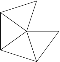
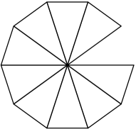
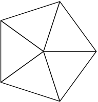
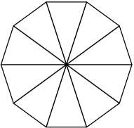
Figure 2. Reference patches $\widehat{\omega}_{N}$ and $\widehat{\omega}^{\prime}_{N}$ in Lemma 10 for $z\in\partial\Gamma$ and $N=4$ as well as $N=9$ resp. for $z\not\in\partial\Gamma$ and $N=5$ as well as $N=10$ (from left to right).

It remains to bound the Lipschitz constants $(L_{2}/L_{1})^{(d+2)/2}$ in (54b) for our particular case of $\kappa(O)$ being a node-patch on a polyhedral surface. To that end, define for any $N\geq 3$ the reference patch $\widehat{\omega}_{N}\subset{\mathbb{R}}^{2}=\mathbb{C}$ to be the compact regular polygon with corners $e^{\frac{2\pi ik}{N}}$, for $k=0,\ldots,N-1$ (where $0$ is an interior point). Moreover, let ${\rm conv}\{\cdot\}$ denote the closed convex hull. Define $\widehat{\omega}_{1}^{\prime}:={\rm conv}\{0,1,i\}$ and, for $N\geq 2$, $\widehat{\omega}_{N}^{\prime}:=\widehat{\omega}_{N+1}\setminus{\rm interior}({\rm conv}\{0,1,e^{\frac{2\pi i}{N+1}}\})$ (where $0$ is a boundary vertex); see Figure 2. The next lemma constructs appropriate uniformly bi-Lipschitz pullbacks to the reference patches. Since the proof is elementary but lengthy, we only sketch it and refer to [ME14] for the details.

Lemma 10.

Let $z\in\mathcal{N}_{\star}$ be some node of a triangulation $\mathcal{T}_{\star}$ of $\Gamma\subset{\mathbb{R}}^{d}$, and let $d=2,3$. Let $N:=\#\{T\in\mathcal{T}_{\star}\colon z\in T\}$ be the number of elements in the node patch $\omega_{\star}(z)$ from (51) and define

$$\widehat{\omega}:=(-1,1)\quad\text{for $d=2$}\quad\text{resp.}\quad\widehat{\omega}:=\begin{cases}\widehat{\omega}_{N}^{\prime}&\text{for }z\in\partial\Gamma,\\ \widehat{\omega}_{N}&\text{for }z\not\in\partial\Gamma,\end{cases}\quad\text{for $d=3$.}$$

Then, there exists

$$\kappa_{z}:\widehat{\omega}\to\omega_{\star}(z)$$

bi-Lipschitz with

$$C^{-1}\,{\rm diam}(\omega_{\star}(z))\leq L_{1}\quad\text{and}\quad L_{2}\leq C\,{\rm diam}(\omega_{\star}(z)).$$ (57)

The constant $C>0$ depends only on $\Gamma$ and the $\gamma$-shape regularity of $\mathcal{T}_{\star}$.

Sketch of proof.

We only sketch the case $d=3$, whereas the simpler case $d=2$ is left to the reader. Let $\widehat{T}_{1},\ldots,\widehat{T}_{N}$ denote the elements in $\widehat{\omega}=\bigcup_{j=1}^{N}\widehat{T}_{j}$ and let $T_{1},\ldots,T_{N}$ denote the elements of $\omega_{\star}(z)=\bigcup_{j=1}^{N}T_{j}$. Without loss of generality, we assume that the numbering of the elements is such that $\#(\widehat{T}_{i}\cap\widehat{T}_{j})=\#(T_{i}\cap T_{j})\in\{1,\infty\}$ for all $1\leq i,j\leq N$. This allows to find a unique affine mapping $\kappa_{j}:\,\widehat{T}_{j}\to T_{j}$ which satisfies

$$\kappa_{j}(0)=z\quad\text{and}\quad\kappa_{j}(\widehat{T}_{j}\cap\widehat{T}_{i})=T_{j}\cap T_{i}\quad\text{for all }i=1,\ldots,N.$$

Define $\kappa:\,\widehat{\omega}\to\omega_{\star}(z)$ as

$$\kappa|_{\widehat{T}_{j}}=\kappa_{j}\quad\text{for all }j=1,\ldots,N.$$

If $z^{\prime}\in(\widehat{T}_{j}\cap\widehat{T}_{i})\setminus\{0\}$, there holds $\kappa_{j}(z^{\prime})\in T_{i}\cap T_{j}$ and $\kappa_{i}(z^{\prime})\in T_{i}\cap T_{j}$ by definition. Since the $\kappa_{j}$ are affine, there holds $\kappa_{i}|_{\widehat{E}}=\kappa_{j}|_{\widehat{E}}$ on $\widehat{E}=\widehat{T}_{i}\cap\widehat{T}_{j}$. This shows that $\kappa$ is well-defined and continuous. Straightforward arguments show that $N$ and the Lipschitz continuity of the $\kappa_{j}$ depend only on the $\gamma$-shape regularity of ${\mathcal{T}}_{\star}$. The Lipschitz continuity (57) of $\kappa$ depends additionally on $\Gamma$. ∎

With this at hand, the proof of Proposition 8 follows.

Proof of Proposition 8.

Using the mapping $\kappa=\kappa_{z}$ from Lemma 10, we can apply Lemma 9 with $O=\widehat{\omega}$ and $\kappa(O)=\omega_{\star}(z)$. This immediately gives

$$|v|_{H^{s}(\omega_{\star}(z))}\simeq{\rm diam}(\omega_{\star}(z))^{(d-1)/2-s}|v\circ\kappa|_{H^{s}(\widehat{\omega})}$$

for all $v\in H^{1}(\omega_{\star}(z))$, $s\in(0,1]$, with constants depending only on the $\gamma$-shape regularity of ${\mathcal{T}}_{\ell}$. On the reference patch, we can use the continuous embedding $H^{1}(\widehat{\omega})\subset H^{s}(\widehat{\omega})$ and Poincaré’s inequality to obtain

$$|v\circ\kappa|_{H^{s}(\widehat{\omega})}=\min_{c\in{\mathbb{R}}}|v\circ\kappa-c|_{H^{s}(\widehat{\omega})}\leq\min_{c\in{\mathbb{R}}}\|v\circ\kappa-c\|_{H^{s}(\widehat{\omega})}\lesssim\min_{c\in{\mathbb{R}}}\|v\circ\kappa-c\|_{H^{1}(\widehat{\omega})}\lesssim|v\circ\kappa|_{H^{1}(\widehat{\omega})}.$$

The hidden constant depends only on $\widehat{\omega}$ and is hence controlled by the $\gamma$-shape regularity of ${\mathcal{T}}_{\ell}$. Combining the last two estimates, we get

$$|v|_{H^{s}(\omega_{\star}(z))} \simeq {\rm diam}(\omega_{\star}(z))^{(d-1)/2-s}|v\circ\kappa|_{H^{s}(\widehat{\omega})}$$

$$\lesssim {\rm diam}(\omega_{\star}(z))^{(d-1)/2-s}|v\circ\kappa|_{H^{1}(\widehat{\omega})}$$

$$\simeq {\rm diam}(\omega_{\star}(z))^{1-s}|v|_{H^{1}(\omega_{\star}(z))}.$$

This concludes the proof. ∎

3.6. Remarks and Extensions

The inverse estimates of [GHS05, Theorem 3.6] and [AFF⁺12, Corollary 3] also apply to higher-order discretizations ${\mathcal{P}}^{p}({\mathcal{T}}_{\star})$ with piecewise polynomials of degree $p\geq 0$ and curved surface triangles (where $\Gamma$ is assumed to be piecewise smooth). Also Proposition 8 can be proved for non-polygonal boundaries. Consequently, the convergence results of Theorem 6 and Theorem 7 also transfer to these settings. Moreover, rectangular elements can be covered.

In [Fae00] the spaces ${\mathcal{P}}^{p}({\mathcal{T}}_{\star})$ are defined by local pullback with the arc-length parametrization. While this is immaterial for piecewise affine boundaries, ${\mathcal{P}}^{p}({\mathcal{T}}_{\star})$ depends on the chosen parametrization for non-affine boundaries. For 2D BEM, this restriction is removed in the recent work [FGP14].

4. Hyper-singular integral equation

4.1. Model problem

We consider the hyper-singular integral equation

$$Au(x)=-\partial_{\boldsymbol{n}(x)}\int_{\Gamma}\partial_{\boldsymbol{n}(y)}G(x-y)\,u(y)\,d\Gamma(y)=F(x)\quad\text{for all }x\in\Gamma$$ (58)

on a relatively open, connected, and polygonal part $\Gamma\subsetneqq\partial\Omega$ of the boundary of a bounded, polyhedral Lipschitz domain $\Omega\subset{\mathbb{R}}^{d}$, $d=2,3$. (The case $\Gamma=\partial\Omega$ is sketched in Section 4.5 below.) For $d=3$, we assume that the boundary of $\Gamma$ (a polygonal curve) is Lipschitz itself. In (58), $G$ denotes the fundamental solution of the Laplacian; see (25). Moreover, $\partial_{\boldsymbol{n}(x)}$ denotes the normal derivative at $x\in\Gamma$ with $\boldsymbol{n}(x)$ the outer unit normal vector of $\Omega$. The reader is referred to, e.g., the monographs [HW08, McL00, SS11, Ste08] for proofs of and details on the following facts: The hyper-singular integral operator $A:{\mathcal{H}}\to{\mathcal{H}}^{*}$ is a continuous linear operator between the fractional-order Sobolev space ${\mathcal{H}}=\widetilde{H}^{1/2}(\Gamma)$ and its dual ${\mathcal{H}}^{*}=H^{-1/2}(\Gamma)$. Duality is understood with respect to the extended $L^{2}(\Gamma)$-scalar product $\langle\cdot\,,\,\cdot\rangle$. Then, the hyper-singular integral operator is also elliptic

$$\langle Av\,,\,v\rangle\geq C_{\rm ell}\,\|v\|_{\widetilde{H}^{1/2}(\Gamma)}^{2}\quad\text{for all }v\in{\mathcal{H}}=\widetilde{H}^{1/2}(\Gamma)$$ (59)

with some constant $C_{\rm ell}>0$ which depends only on $\Gamma$. Thus, $A$ meets all assumptions of Section 2, and $\|v\|_{A}^{2}:=\langle Av\,,\,v\rangle$ even defines an equivalent Hilbert norm on ${\mathcal{H}}$.

4.2. Discretization

Let ${\mathcal{T}}_{\star}$ be a $\gamma$-shape regular triangulation of $\Gamma$ as defined in Section 3.2. With ${\mathcal{X}}_{\star}=\widetilde{\SS}^{1}({\mathcal{T}}_{\star}):={\mathcal{P}}^{1}({\mathcal{T}}_{\star})\cap\widetilde{H}^{1/2}(\Gamma)$ being the space of ${\mathcal{T}}_{\star}$-piecewise affine, globally continuous functions which vanish at the boundary of $\Gamma$, we now consider the Galerkin formulation (8).

4.3. Weighted-residual error estimator

For given right-hand side $F\in L^{2}(\Gamma)$, the residual $F-AU_{\star}(F)\in H^{-1/2}(\Gamma)$ has additional regularity $F-AU_{\star}\in L^{2}(\Gamma)$, since $A:\widetilde{H}^{1/2+s}(\Gamma)\to H^{-1/2+s}(\Gamma)$ is stable for $-1/2\leq s\leq 1/2$ (but not isomorphic for $s=\pm 1/2$). It is proved in [CMPS04] that

$$\|u(F)-U_{\star}(F)\|_{\widetilde{H}^{1/2}(\Gamma)}\simeq\|F-AU_{\star}(F)\|_{H^{-1/2}(\Gamma)}\lesssim\|h_{\star}^{1/2}(F-AU_{\star}(F))\|_{L^{2}(\Gamma)}=:\eta_{\star}(F).$$ (60)

Overall, this proves the reliability estimate

$$\|u(F)-U_{\star}(F)\|_{\widetilde{H}^{1/2}(\Gamma)}\leq\widetilde{C}_{\rm rel}\,\eta_{\star}(F),$$ (61)

and the constant $\widetilde{C}_{\rm rel}>0$ depends only on $\Gamma$ and the $\gamma$-shape regularity (27) of ${\mathcal{T}}_{\star}$. In particular, the weighted-residual error estimator can be localized via

$$\eta_{\star}(F)=\Big{(}\sum_{T\in{\mathcal{T}}_{\star}}\eta_{\star}(F;T)^{2}\Big{)}^{1/2}\text{ with }\eta_{\star}(F;T)={\rm diam}(T)^{1/2}\|F-AU_{\star}(F)\|_{L^{2}(T)}.$$ (62)

Recently, convergence of Algorithm 2 has been shown even with quasi-optimal rates, if $\eta_{\ell}(F)=\mu_{\ell}(F)$ is used for marking (13), see [Gan13, FFK⁺13b]. We stress that our approach with $\eta_{\ell}(F)=\rho_{\ell}(F)=\mu_{\ell}(F)$ would also give convergence $\eta_{\ell}(F)\to 0$ as $\ell\to\infty$. Since this is, however, a much weaker result than that of [Gan13], we omit the details.

4.4. Two-level error estimator

Let $\widehat{\mathcal{T}}_{\star}$ denote the uniform refinement of ${\mathcal{T}}_{\star}$. Let $\widehat{\mathcal{N}}_{\star}$ be the corresponding set of nodes. Let $z_{T,j}\in T\cap\widehat{\mathcal{N}}_{\star}$, $j=1,\ldots,D$ denote the new nodes of the uniform refinement $\widehat{\mathcal{T}}_{\star}$ within $T$. Let $\{v_{T,1},\dots,v_{T,D}\}\subset\SS^{1}(\widehat{\mathcal{T}}_{\star})$ denote the fine-mesh hat functions which satisfy $v_{T,j}(z_{T,j})=1$ and $v_{T,j}(z)=0$ for all $z\in\widehat{\mathcal{N}}_{\star}\backslash\{z_{T,j}\}$. We note that (in dependence of the chosen mesh-refinement) usually $D=1$ for $d=2$ and $D=3$ for $d=3$. In this setting, the two-level error estimator has first been proposed by [MS00]. Its local contributions read

$$\mu_{\star}(F;T)^{2}=\sum_{j=1}^{D}\mu_{\star,j}(F;T)^{2}\quad\text{with}\quad\mu_{\star,j}(F;T)=\begin{cases}\frac{\langle F-AU_{\star}(F)\,,\,v_{T,j}\rangle}{\langle Av_{T,j}\,,\,v_{T,j}\rangle^{1/2}}&\text{for }z_{T,j}\notin\partial\Gamma,\\ 0&\text{otherwise}.\end{cases}$$ (63)

Put differently, we test the residual $F-AU_{\star}(F)\in H^{-1/2}(\Gamma)$ with the additional basis functions from $\widetilde{\SS}^{1}(\widehat{\mathcal{T}}_{\star})\backslash\widetilde{\SS}^{1}({\mathcal{T}}_{\star})$. This quantity is appropriately scaled by the corresponding energy norm $\|v_{T,j}\|_{H^{-1/2}(\Gamma)}\simeq\langle Av_{T,j}\,,\,v_{T,j}\rangle^{1/2}=\|v_{T,j}\|_{A}$. Note that unlike the weighted-residual error estimator $\eta_{\star}(\cdot)$, the two-level error estimator $\mu_{\star}(F)$ is well-defined under minimal regularity $F\in H^{-1/2}(\Gamma)$ of the given right-hand side.

The two-level estimator $\mu_{\star}(\cdot)$ is known to be efficient [MS00, MMS97, HMS01, EH06, EFGP13, AFF⁺14]

$$\mu_{\star}(F)\leq C_{\rm eff}\,\|u(F)-U_{\star}(F)\|_{\widetilde{H}^{1/2}(\Gamma)},$$ (64)

while reliability

$$\|u(F)-U_{\star}(F)\|_{\widetilde{H}^{1/2}(\Gamma)}\leq C_{\rm rel}\,\mu_{\star}(F)$$ (65)

holds under [MS00, MMS97, HMS01, EH06] and is even equivalent to [EFGP13, AFF⁺14] the saturation assumption

$$\|u(F)-\widehat{U}_{\star}(F)\|_{A}\leq q_{\rm sat}\,\|u(F)-U_{\star}(F)\|_{A}$$ (66)

in the energy norm $\|\cdot\|_{A}\simeq\|\cdot\|_{\widetilde{H}^{1/2}(\Gamma)}$. Here, $0<q_{\rm sat}<1$ is a uniform constant, and $\widehat{U}_{\star}(F)$ is the Galerkin solution with respect to the uniform refinement $\widehat{\mathcal{T}}_{\star}$ of ${\mathcal{T}}_{\star}$. The constant $C_{\rm eff}>0$ depends only on $\Gamma$ and $\gamma$-shape regularity of ${\mathcal{T}}_{\star}$, while $C_{\rm rel}>0$ additionally depends on the saturation constant $q_{\rm sat}$. (The saturation assumption (66) for the $\widetilde{H}^{1/2}$-norm $\|\cdot\|_{A}=\|\cdot\|_{\widetilde{H}^{1/2}/(\Gamma)}$ implies reliability (65), but is not necessary though.)

Theorem 11.

Suppose that the two-level error estimator (63) is used for marking (13). Suppose that the mesh-refinement guarantees uniform $\gamma$-shape regularity of the meshes ${\mathcal{T}}_{\ell}$ generated, as well as that all marked elements $T\in{\mathcal{M}}_{\ell}$ are refined into sons $T^{\prime}\in{\mathcal{T}}_{\ell+1}$ with $|T^{\prime}|\leq\kappa\,|T|$ with some uniform constant $0<\kappa<1$. Then, Algorithm 2 guarantees

$$\mu_{\ell}(F)\to 0\quad\text{as }\ell\to\infty.$$ (67)

for all $F\in H^{1/2}(\Gamma)$.

Proof.

With Proposition 5, it remains to verify the abstract assumptions (A1)–(A3).

$\bullet$ We use the modified mesh-width function $\widetilde{h}_{\ell}$ from the proof of Theorem 7 and define the modified weighted-residual error estimator

$$C_{\rm mesh}^{-1/2}\,\eta_{\ell}(F;T)\leq\rho_{\ell}(F;T):=\|\widetilde{h}_{\ell}^{1/2}(F-AU_{\ell}(F))\|_{L^{2}(T)}\leq\eta_{\ell}(F;T).$$ (68)

Arguing analogously to the proof of Theorem 6, we verify contraction (A2). The only difference is that instead of (41), we use the inverse-type estimate

$$\|h_{\ell}^{1/2}AV_{\ell}\|_{L^{2}(\Gamma)}\leq C_{\rm inv}\,\|V_{\ell}\|_{\widetilde{H}^{1/2}(\Gamma)}\text{for all }V_{\ell}\in\widetilde{\SS}^{1}({\mathcal{T}}_{\ell}),$$ (69)

where the constant $C_{\rm inv}>0$ depends only on $\Gamma$ and $\gamma$-shape regularity of ${\mathcal{T}}_{\ell}$; see [AFF⁺12, Corollary 3].

$\bullet$ It is proved in [CMPS04, Theorem 5.4] that

$$\mu_{\ell,j}(F;T)\lesssim\|h_{\ell}^{1/2}(F-AU_{\ell})\|_{L^{2}({\rm supp}(v_{T,j}))},$$

where the hidden constant depends only on $\Gamma$ and $\gamma$-shape regularity of ${\mathcal{T}}_{\ell}$. By definition (60) of the weighted-residual error estimator and (68), this implies

$$\mu_{\ell}(F;T)^{2}\lesssim\sum_{{T^{\prime}\in{\mathcal{T}}_{\ell}}\atop{T^{\prime}\cap T\neq\emptyset}}\eta_{\ell}(F;T)^{2}\simeq\sum_{{T^{\prime}\in{\mathcal{T}}_{\ell}}\atop{T^{\prime}\cap T\neq\emptyset}}\rho_{\ell}(F;T)^{2}.$$

Using the notation from the proof of Theorem 7, this yields (A1) with ${\mathcal{R}}_{\ell}:=\omega_{\ell}({\mathcal{M}}_{\ell})$ being the marked elements plus one additional layer of elements; see (48) for the definition of $\omega_{\ell}(\cdot)=\omega_{\ell}^{1}(\cdot)$.

$\bullet$ Finally, stability (A3) follows from efficiency (64); see (19). ∎

4.5. Remarks and Extensions

The inverse estimate (69) of [AFF⁺12, Corollary 3] also applies to higher-order discretizations $\widetilde{\SS}^{p}({\mathcal{T}}_{\star}):={\mathcal{P}}^{p}({\mathcal{T}}_{\star})\cap\widetilde{H}^{1/2}(\Gamma)$ with piecewise polynomials of degree $p\geq 1$ and curved surface triangles. Consequently, the convergence results of Theorem 6 and Theorem 7 also transfer to these settings. Moreover, also rectangular elements can be covered.

If the boundary $\Gamma$ is closed, i.e. $\Gamma=\partial\Omega$, the hypersingular operator $W:H^{1/2}_{0}(\Gamma)\to H^{-1/2}_{0}(\Gamma)$ is well-defined and elliptic, where $H^{\pm 1/2}_{0}(\Gamma)=\big{\{}v\in H^{\pm 1/2}(\Gamma)\,:\,\langle v\,,\,1\rangle=0\big{\}}$. Therefore, well-posedness of (58) requires the compatibility condition $F\in H^{-1/2}_{0}(\Gamma)$. On the one hand, one may formulate the weak formulation of (58) as well as its Galerkin discretization with respect to the subspaces ${\mathcal{H}}=H^{1/2}_{0}(\Gamma)$ and ${\mathcal{X}}_{\star}={\mathcal{P}}^{p}({\mathcal{T}}_{\star})\cap H^{1/2}_{0}(\Gamma)$. On the other hand, one can choose the full space ${\mathcal{H}}=H^{1/2}(\Gamma)$ and ${\mathcal{X}}_{\star}={\mathcal{P}}^{p}({\mathcal{T}}_{\star})\cap H^{1/2}(\Gamma)$ and consider the naturally stabilized formulation

$$a(u,v):=\langle Au\,,\,v\rangle+\langle u\,,\,1\rangle\langle v\,,\,1\rangle=\langle F\,,\,v\rangle\quad\text{for all }v\in{\mathcal{H}}=H^{1/2}(\Gamma).$$ (70)

The compatibility condition on $F$ and $1\in\SS^{1}({\mathcal{T}}_{\star})={\mathcal{P}}^{1}({\mathcal{T}}_{\star})\cap H^{1/2}(\Gamma)$ ensure that both, the exact solution $u=u(F)\in H^{1/2}(\Gamma)$ of (70) as well as the Galerkin approximation $U_{\star}=U_{\star}(F)\in\SS^{1}({\mathcal{T}}_{\star})$, satisfy $\langle u(F)\,,\,1\rangle=0=\langle U_{\star}(F)\,,\,1\rangle$, i.e., $u(F)\in H^{1/2}_{0}(\Gamma)$ as well as $U_{\star}(F)\in{\mathcal{P}}^{1}({\mathcal{T}}_{\star})\cap H^{1/2}_{0}(\Gamma)$. In either case, the weighted-residual error estimator coincides with (60) and the two-level error estimator is obtained analogously to Section 4.4. For the two-level error estimator, we refer, e.g., to [EFGP13] for the $H^{1/2}_{0}(\Gamma)$-based discretization and to [AFF⁺14] for the stabilized approach. In any case, Theorem 11 holds accordingly.

5. FEM-BEM Coupling

5.1. Model problem

Let $\Omega\subset{\mathbb{R}}^{d}$ be a Lipschitz domain with polygonal boundary $\Gamma:=\partial\Omega$, $d=2,3$. Let $B:{\mathbb{R}}^{d}\to{\mathbb{R}}^{d}$ be Lipschitz continuous

$$|Bx-By|\leq C_{\ref{constlipB}}|x-y|\quad\text{for all }x,y\in{\mathbb{R}}^{d}$$ (71)

for some $C_{\ref{constlipB}}>0$. In addition, we assume that the induced operator $B:L^{2}(\Omega)^{d}\to L^{2}(\Omega)^{d}$, $(B\boldsymbol{f})(x):=B(\boldsymbol{f}(x))$ is strongly monotone

$$\int_{\Omega}(B\boldsymbol{f}-B\boldsymbol{g})\cdot(\boldsymbol{f}-\boldsymbol{g})\,d\Omega\geq C_{\ref{constmonB}}\|\boldsymbol{f}-\boldsymbol{g}\|_{L^{2}(\Omega)}^{2}\quad\text{for all }\boldsymbol{f},\boldsymbol{g}\in L^{2}(\Omega)^{d}$$ (72)

with monotonicity constant $C_{\ref{constmonB}}>1/4$. (Arguing as in [OS13], this assumption can be sharpened to $C_{\ref{constmonB}}>q_{\mathfrak{K}}/4$, where $1/2\leq q_{\mathfrak{K}}<1$ is the contraction constant of the double-layer integral operator.) We consider a possibly nonlinear Laplace transmission problem which is reformulated in terms of the Johnson-Nédélec FEM-BEM coupling [JN80]: For given data $(f,u_{0},\phi_{0})\in L^{2}(\Omega)\times H^{1/2}(\Gamma)\times H^{-1/2}(\Gamma)$, find $\boldsymbol{u}=(u,\phi)\in{\mathcal{H}}:=H^{1}(\Omega)\times H^{-1/2}(\Gamma)$ such that

$$\int_{\Omega}B\nabla u\cdot\nabla v\,d\Omega-\int_{\Gamma}\phi v\,d\Gamma =\int_{\Omega}fv\,d\Omega+\int_{\Gamma}\phi_{0}v\,d\Gamma,$$ (73a)

$$\int_{\Gamma}\big{(}(1/2-\mathfrak{K})u+\mathfrak{V}\phi\big{)}\psi\,d\Gamma =\int_{\Gamma}(1/2-\mathfrak{K})u_{0}\psi\,d\Gamma$$ (73b)

for all $\boldsymbol{v}=(v,\psi)\in{\mathcal{H}}$. Here, $\mathfrak{V}\psi(x):=\int_{\Gamma}G(x-y)\psi(y)\,d\Gamma(y)$ is the simple-layer integral operator and $\mathfrak{K}v(x):=\int_{\Gamma}\partial_{\boldsymbol{n}(y)}G(x-y)v(y)\,d\Gamma(y)$ is the double-layer integral operator, with $G$ being the fundamental solution (25) of the Laplacian. To ensure ellipticity of $\mathfrak{V}:H^{-1/2}(\Gamma)\to H^{1/2}(\Gamma)=(H^{-1/2}(\Gamma))^{*}$, we assume ${\rm diam}(\Omega)<1$ for $d=2$ by scaling; see also Section 3. Let $\|\boldsymbol{v}\|_{{\mathcal{H}}}^{2}:=\|v\|_{H^{1}(\Omega)}^{2}+\|\psi\|_{H^{-1/2}(\Gamma)}^{2}$ for $\boldsymbol{v}=(v,\psi)\in{\mathcal{H}}$ denote the canonical product norm on ${\mathcal{H}}$.

The left-hand side of (73) gives rise to some operator $A:{\mathcal{H}}\to{\mathcal{H}}^{*}$. The right-hand side of (73) gives rise to some $F\in{\mathcal{H}}^{*}$ which depends on the given data $f,u_{0},\phi_{0}$. Then, (73) can equivalently be reformulated by (8) with ${\mathcal{X}}_{\star}={\mathcal{H}}$. Note that $\langle\phi\,,\,\psi\rangle_{\mathfrak{V}}:=\int_{\Gamma}\psi\mathfrak{V}\phi\,d\Gamma$ defines a scalar product on $H^{-1/2}(\Gamma)$ with induced norm $\|\cdot\|_{\mathfrak{V}}^{2}:=\langle\cdot\,,\,\cdot\rangle_{\mathfrak{V}}$. The following proposition states that the FEM-BEM formulation (73) fits into the abstract frame of Section 2.

Proposition 12.

The operator $A:{\mathcal{H}}\to{\mathcal{H}}^{*}$ associated with the left-hand side of (73) is bi-Lipschitz continuous (6), where $C_{\rm cont}>0$ depends only on $C_{\ref{constlipB}}$, $C_{\ref{constmonB}}$, and $\Omega$. Let $F\in{\mathcal{H}}^{*}$ and let ${\mathcal{X}}_{\star}$ be a closed subspace of ${\mathcal{H}}$. Provided that $(0,1)\in{\mathcal{X}}_{\star}$, i.e. ${\mathcal{X}}_{00}={\rm span}\{(0,1)\}$, the variational formulation (8) admits a unique solution $\mathbf{U}_{\star}(F)=(U_{\star}(F),\Phi_{\star}(F))\in{\mathcal{X}}_{\star}$, and there holds the Céa lemma (10). The constant $C_{\mbox{\rm\scriptsize C\'{e}a}}>0$ depends only on $C_{\ref{constlipB}}$, $C_{\ref{constmonB}}$, and $\Omega$.

Sketch of proof.

The statements on unique solvability and Céa-type quasi-optimality are proved in [AFF⁺13a]; see also [Say09] for the linear Laplace transmission problem, where $B$ is the identity. It only remains to show that $A$ is bi-Lipschitz. The upper bound in (6) follows from Lipschitz continuity (71) of $B$ and the continuity of the boundary integral operators $\mathfrak{V}:H^{-1/2}(\Gamma)\to H^{1/2}(\Gamma)$ and $\mathfrak{K}:H^{1/2}(\Gamma)\to H^{1/2}(\Gamma)$. For the lower bound in (6), we use the definition of the dual norm

$$\|A\boldsymbol{u}-A\boldsymbol{v}\|_{{\mathcal{H}}^{*}}=\sup\limits_{\boldsymbol{w}=(w,\chi)\in{\mathcal{H}}\backslash\{(0,0)\}}\frac{|\langle A\boldsymbol{u}-A\boldsymbol{v}\,,\,\boldsymbol{w}\rangle|}{\|\boldsymbol{w}\|_{{\mathcal{H}}}}$$

For $\boldsymbol{u}=(u,\phi),\boldsymbol{v}=(v,\psi)\in{\mathcal{H}}$, we choose $\boldsymbol{w}=\boldsymbol{u}-\boldsymbol{v}+(0,1)\int_{\Gamma}(\tfrac{1}{2}-\mathfrak{K})(u-v)+\mathfrak{V}(\phi-\psi)\,d\Gamma$. By continuity of $\mathfrak{V}$ and $\mathfrak{K}$, it follows $\|\boldsymbol{w}\|_{{\mathcal{H}}}\lesssim\|\boldsymbol{u}-\boldsymbol{v}\|_{{\mathcal{H}}}$, where the hidden constant depends only on $\Omega$. Moreover, $\boldsymbol{w}=(0,0)$ implies that $u=v$ and $\phi-\psi=-\langle\phi-\psi\,,\,1\rangle_{\mathfrak{V}}=:c\in{\mathbb{R}}$ is constant. With this identity, it follows $0=(1+\langle 1\,,\,1\rangle_{\mathfrak{V}})c$. Ellipticity of $\mathfrak{V}$ proves $0=c=\phi-\psi$, i.e., $\boldsymbol{w}=0$ yields $\boldsymbol{u}=\boldsymbol{v}$.

The theory of implicit stabilization provided in [AFF⁺13a] shows $\langle A\boldsymbol{u}-A\boldsymbol{v}\,,\,\boldsymbol{w}\rangle\gtrsim\|\boldsymbol{u}-\boldsymbol{v}\|_{{\mathcal{H}}}^{2}$, where the hidden constant depends only on $C_{\ref{constmonB}}$, and $\Omega$. For $\boldsymbol{u}\neq\boldsymbol{v}$, we altogether obtain ${|\langle A\boldsymbol{u}-A\boldsymbol{v}\,,\,\boldsymbol{w}\rangle|}/{\|\boldsymbol{w}\|_{{\mathcal{H}}}}\geq C_{\rm cont}^{-1}\|\boldsymbol{u}-\boldsymbol{v}\|_{{\mathcal{H}}}$, where $C_{\rm cont}>0$ depends only on $C_{\ref{constlipB}},C_{\ref{constmonB}}$, and $\Omega$. ∎

5.2. Discretization

Let ${\mathcal{T}}_{\star}^{\Omega}$ be a $\gamma$-shape regular triangulation of $\Omega$ into triangles for $d=2$ resp. tetrahedrons for $d=3$. Here, $\gamma$-shape regularity means

$$\sup\limits_{T\in{\mathcal{T}}_{\star}^{\Omega}}\frac{{\rm diam}(T)^{d}}{|T|}\leq\gamma<\infty$$ (74)

with $|\cdot|$ being the $d$-dimensional volume measure. Suppose that ${\mathcal{T}}_{\star}^{\Omega}$ is regular in the sense of Ciarlet, i.e., ${\mathcal{T}}_{\star}^{\Omega}$ admits no hanging nodes. Let ${\mathcal{T}}_{\star}^{\Gamma}:={\mathcal{T}}_{\star}^{\Omega}|_{\Gamma}$ be the triangulation of $\Gamma$ which is induced by ${\mathcal{T}}_{\star}^{\Omega}$. Note that ${\mathcal{T}}_{\star}^{\Gamma}$ then is $\widetilde{\gamma}$-shape regular in the sense of (27), where $\widetilde{\gamma}>0$ depends only on $\gamma$. Moreover, for $d=3$, ${\mathcal{T}}_{\star}^{\Gamma}$ is regular in the sense of Ciarlet as well. We formally consider ${\mathcal{T}}_{\star}:={\mathcal{T}}_{\star}^{\Omega}\cup{\mathcal{T}}_{\star}^{\Gamma}$ with the abstract notation of Section 2. Let $\SS^{1}({\mathcal{T}}_{\star}^{\Omega})$ be the space of piecewise affine, globally continuous functions on ${\mathcal{T}}_{\star}^{\Omega}$ and ${\mathcal{P}}^{0}({\mathcal{T}}_{\star}^{\Gamma})$ be the space of all ${\mathcal{T}}_{\star}^{\Gamma}$-piecewise constant functions. With ${\mathcal{X}}_{\star}:=\SS^{1}({\mathcal{T}}_{\star}^{\Omega})\times{\mathcal{P}}^{0}({\mathcal{T}}_{\star}^{\Gamma})$, we now consider the Galerkin formulation (8). The discrete solution with respect to ${\mathcal{X}}_{\star}$ will be denoted by $\boldsymbol{U}_{\star}=(U_{\star},\Phi_{\star})$.

5.3. Weighted-residual error estimator

Assume additional regularity $(f,u_{0},\phi_{0})\in L^{2}(\Omega)\times H^{1}(\Gamma)\times L^{2}(\Gamma)$. Following [CS95a], it is proved in [AFKP12] for linear problems and in [AFF⁺13a] for strongly monotone problems that

$$\|\boldsymbol{u}(F)-\boldsymbol{U}_{\star}(F)\|_{{\mathcal{H}}}\simeq\|F-A\boldsymbol{U}_{\star}(F)\|_{{\mathcal{H}}^{*}}\lesssim\eta_{\star}(F),$$ (75)

where the error estimator $\eta_{\star}(F)^{2}:=\sum_{T\in{\mathcal{T}}_{\star}}\eta_{\star}(F;T)^{2}$ is defined by

$$\begin{split}\eta_{\star}(F;T)^{2}&:={\rm diam}(T)^{2}\,\|f\|_{L^{2}(T)}^{2}\\ &+\!{\rm diam}(T)\,\Big{(}\|[B\nabla U_{\star}\cdot\boldsymbol{n}]\|_{L^{2}(\partial T\backslash\Gamma)}^{2}+\|\phi_{0}+\Phi_{\star}-B\nabla U_{\star}\cdot\boldsymbol{n}\|_{L^{2}(\partial T\cap\Gamma)}^{2}\Big{)}\end{split}$$ (76a)

for $$T\in{\mathcal{T}}_{\star}^{\Omega}$$ resp.

$$\eta_{\star}(F;T)^{2} :={\rm diam}(T)\,\|\nabla_{\Gamma}\big{(}(1/2-\mathfrak{K})(U_{\star}-u_{0})+\mathfrak{V}\Phi_{\star}\big{)}\|_{L^{2}(T)}^{2}$$ (76b)

for $T\in{\mathcal{T}}_{\star}^{\Gamma}$. Here, $[B\nabla U_{\star}\cdot\boldsymbol{n}]$ denotes the jump of $B\nabla U\cdot\boldsymbol{n}$ across interior facets $E$, where $E=T_{+}\cap T_{-}$ for some $T_{+},T_{-}\in{\mathcal{T}}_{\star}^{\Omega}$ with $T_{+}\neq T_{-}$. By means of the estimator reduction principle [AFLP12], it follows that Algorithm 2 converges for $\eta_{\ell}(F)=\mu_{\ell}(F)$; see [AFF⁺13a].

5.4. Two-level error estimator

Two-level error estimators for the adaptive coupling of FEM and BEM have first been proposed in [MS99]. Let $\widehat{\mathcal{T}}_{\star}^{\Omega}$ denote the uniform refinement of ${\mathcal{T}}_{\star}^{\Omega}$. Let $\widehat{\mathcal{N}}_{\star}^{\Omega}$ be the corresponding set of nodes and $\widehat{\mathcal{T}}_{\star}^{\Gamma}:=\widehat{\mathcal{T}}_{\star}^{\Omega}|_{\Gamma}$ be the induced triangulation of $\Gamma$. For each element $T\in{\mathcal{T}}_{\star}^{\Omega}$, let $z_{T,j}\in T\cap\widehat{\mathcal{N}}_{\star}^{\Omega}$, $j=1,\dots,D^{\Omega}$ denote the new nodes of the uniform refinement $\widehat{\mathcal{T}}_{\star}^{\Omega}$ within $T$. Let $v_{T,j}\in\SS^{1}(\widehat{\mathcal{T}}_{\star}^{\Omega})$ denote the fine-mesh hat functions, which satisfy $v_{T,j}(z_{T,j})=1$ and $v_{T,j}(z)=0$ for all $z\in\widehat{\mathcal{N}}_{\star}^{\Omega}\backslash\{z_{T,j}\}$. Moreover, let $\{\chi_{T},\psi_{T,j},\dots,\psi_{T,D^{\Gamma}}\}$ denote a basis of ${\mathcal{P}}^{0}(\widehat{\mathcal{T}}_{\star}^{\Gamma}|_{T})$ for each element $T\in{\mathcal{T}}_{\star}^{\Gamma}$, with $\chi_{T}$ being the characteristic function on $T$ and $\int_{\Gamma}\psi_{T,j}\,d\Gamma=0$. Then, the two-level estimator $\mu_{\star}^{2}:=\sum_{T\in{\mathcal{T}}_{\star}}\mu_{\star}(F;T)^{2}$ is defined by

$$\mu_{\star}(F;T)^{2}:=\sum_{j=1}^{D^{\Omega}}\mu_{\star,j}(F;T)^{2}\quad\text{with}\quad\mu_{\star,j}(F;T):=\frac{\langle F-A\boldsymbol{U}_{\star}(F)\,,\,(v_{T,j},0)\rangle}{\|v_{T,j}\|_{H^{1}(\Omega)}}$$ (77a)

for $$T\in{\mathcal{T}}_{\star}^{\Omega}$$ and

$$\mu_{\star}(F;T)^{2}:=\sum_{j=1}^{D^{\Gamma}}\mu_{\star,j}(F;T)^{2}\quad\text{with}\quad\mu_{\star,j}(F;T):=\frac{\langle F-A\boldsymbol{U}_{\star}(F)\,,\,(0,\psi_{T,j})\rangle}{\|\psi_{T,j}\|_{\mathfrak{V}}}$$ (77b)

for $$T\in{\mathcal{T}}_{\star}^{\Gamma}$$.

Note that unlike the weighted-residual error estimator (76), the two-level error estimator (77) does not require additional regularity of the data, but only $(f,u_{0},\phi_{0})\in L^{2}(\Omega)\times H^{1/2}(\Gamma)\times H^{-1/2}(\Gamma)$.

The two-level estimator $\mu_{\star}$ is known to be efficient

$$\mu_{\star}(F)\leq C_{\rm eff}\|\boldsymbol{u}(F)-\boldsymbol{U}_{\star}(F)\|_{{\mathcal{H}}},$$ (78)

while reliability

$$\|\boldsymbol{u}(F)-\boldsymbol{U}_{\star}(F)\|_{{\mathcal{H}}}\leq C_{\rm rel}\mu_{\star}(F)$$ (79)

holds under the saturation assumption

$$\|\boldsymbol{u}(F)-\widehat{\boldsymbol{U}}_{\star}(F)\|_{{\mathcal{H}}}\leq q_{\rm sat}\|\boldsymbol{u}(F)-\boldsymbol{U}_{\star}(F)\|_{{\mathcal{H}}};$$ (80)

see [AFKP12] for the linear Johnson-Nédélec coupling and the seminal work [MS99] for some non-linear symmetric coupling. Here, $\widehat{\boldsymbol{U}}_{\star}(F)$ denotes the Galerkin solution with respect to the uniform refinement $(\widehat{\mathcal{T}}_{\star}^{\Omega},\widehat{\mathcal{T}}_{\star}^{\Gamma})$ of $({\mathcal{T}}_{\star}^{\Omega},{\mathcal{T}}_{\star}^{\Gamma})$, and $0<q_{\rm sat}<1$ is a uniform constant. The details are left to the reader.

Theorem 13.

Suppose that the two-level error estimator (77) is used for marking (13). Suppose that the mesh-refinement guarantees uniform $\gamma$-shape regularity of the meshes ${\mathcal{T}}_{\ell}^{\Omega},{\mathcal{T}}_{\ell}^{\Gamma}$ generated, as well as that all marked elements $T\in{\mathcal{M}}_{\ell}\subseteq{\mathcal{T}}_{\ell}^{\Omega}\cup{\mathcal{T}}_{\ell}^{\Gamma}$ are refined into sons $T^{\prime}\in{\mathcal{T}}_{\ell+1}={\mathcal{T}}_{\ell+1}^{\Omega}\cup{\mathcal{T}}_{\ell+1}^{\Gamma}$ with $|T^{\prime}|\leq\kappa\,|T|$ with some uniform constant $0<\kappa<1$, where $|\cdot|$ denotes the $d$-dimensional volume measure for $T\in{\mathcal{T}}_{\ell}^{\Omega}$ resp. the $(d-1)$-dimensional surface measure for $T\in{\mathcal{T}}_{\ell}^{\Gamma}$. Then, Algorithm 2 guarantees

$$\mu_{\ell}(F)\to 0\quad\text{as }\ell\to\infty$$ (81)

for all $F\in{\mathcal{H}}^{*}$.

Our proof of Theorem 13 requires the following two results, which essentially state stability of two-level decompositions of the discrete space $\widehat{\mathcal{X}}_{\ell}:=\SS^{1}(\widehat{\mathcal{T}}_{\ell}^{\Omega})\times{\mathcal{P}}^{0}(\widehat{\mathcal{T}}_{\ell}^{\Gamma})$. The following lemma is a consequence of [Yse86, Theorem 4.1] and explicitly stated in [MS99, Lemma 3.1]. It provides a hierarchical splitting of $\SS^{1}(\widehat{\mathcal{T}}_{\ell}^{\Omega})$.

Lemma 14.

Let $P_{\ell}^{\Omega}:H^{1}(\Omega)\to\SS^{1}({\mathcal{T}}_{\ell}^{\Omega})$ and $P_{T,j}^{\Omega}:H^{1}(\Omega)\to\mathrm{span}\{v_{T,j}\}$ denote the $H^{1}$-orthogonal projections. For $\widehat{V}_{\ell}\in\SS^{1}(\widehat{\mathcal{T}}_{\ell}^{\Omega})$, it then holds

$$C_{\ref{constdecompOmega}}^{-1}\|\widehat{V}_{\ell}\|_{H^{1}(\Omega)}^{2}\leq\|P_{\ell}^{\Omega}\widehat{V}_{\ell}\|_{H^{1}(\Omega)}^{2}+\sum_{T\in{\mathcal{T}}_{\ell}^{\Omega}}\sum_{j=1}^{D^{\Omega}}\|P_{j,T}^{\Omega}\widehat{V}_{\ell}\|_{H^{1}(\Omega)}^{2}\leq C_{\ref{constdecompOmega}}\|\widehat{V}_{\ell}\|_{H^{1}(\Omega)}^{2}.$$ (82)

The constant $C_{\ref{constdecompOmega}}>0$ depends only on $\Omega$ and the $\gamma$-shape regularity of ${\mathcal{T}}_{\ell}^{\Omega}$. ∎

The following lemma is found in [EFLFP09, Proposition 4.5] and provides a hierarchical splitting of ${\mathcal{P}}^{0}(\widehat{\mathcal{T}}_{\ell}^{\Gamma})$. Although [EFLFP09] is only formulated for 2D BEM, the results and proofs hold verbatim for 3D. (For 3D BEM and uniform meshes, the claim is already found in [MSW98]).

Lemma 15.

Let $P_{\ell}^{\Gamma}:H^{-1/2}(\Gamma)\to{\mathcal{P}}^{0}({\mathcal{T}}_{\ell}^{\Gamma})$ and $P_{T,j}^{\Gamma}:H^{-1/2}(\Gamma)\to\mathrm{span}\{\psi_{T,j}\}$ denote the orthogonal projections with respect to the $\mathfrak{V}$-induced scalar product $\langle\cdot\,,\,\cdot\rangle_{\mathfrak{V}}$ on $H^{-1/2}(\Gamma)$. For $\widehat{\Psi}_{\ell}\in{\mathcal{P}}^{0}(\widehat{\mathcal{T}}_{\ell}^{\Gamma})$, it then holds

$$C_{\ref{constdecompGamma}}^{-1}\|\widehat{\Psi}_{\ell}\|_{\mathfrak{V}}^{2}\leq\|P_{\ell}^{\Gamma}\widehat{\Psi}_{\ell}\|_{\mathfrak{V}}^{2}+\sum_{T\in{\mathcal{T}}_{\ell}^{\Gamma}}\sum_{j=1}^{D^{\Gamma}}\|P_{j,T}^{\Gamma}\widehat{\Psi}_{\ell}\|_{\mathfrak{V}}^{2}\leq C_{\ref{constdecompGamma}}\|\widehat{\Psi}_{\ell}\|_{\mathfrak{V}}^{2}.$$ (83)

The constant $C_{\ref{constdecompGamma}}>0$ depends only on $\Gamma$ and the $\gamma$-shape regularity of ${\mathcal{T}}_{\ell}^{\Gamma}$. ∎

Proof of Theorem 13.

The proof is similar to the one of Theorem 6 and relies on the verification of (A1)–(A3) to apply Proposition 5. For patches, we use the notation (48) from the proof of Theorem 7, but now defined for volume elements, i.e., ${\mathcal{T}}_{\ell}^{\Omega}$ instead of ${\mathcal{T}}_{\ell}^{\Gamma}={\mathcal{T}}_{\ell}$ in (48).

$\bullet$ We define the equivalent mesh-size function $\widetilde{h}_{\ell}:\Omega\to{\mathbb{R}}$ as in (49) in the proof of Theorem 7, but now for volume elements $T\in{\mathcal{T}}_{\ell}^{\Omega}$, as well as $\widetilde{h}_{\ell}(T):=|T|^{1/(d-1)}$ for boundary elements $T\in{\mathcal{T}}_{\ell}^{\Gamma}$. The auxiliary estimator $\rho_{\ell}(F)^{2}:=\sum_{T\in{\mathcal{T}}_{\ell}}\rho_{\ell}(F;T)^{2}$ is defined by

$$\begin{split}\rho_{\ell}(F;T)^{2}:=&\|\widetilde{h}_{\ell}f\|_{L^{2}(T)}^{2}+\|\widetilde{h}_{\ell}^{1/2}[B\nabla U_{\ell}\cdot\boldsymbol{n}]\|_{L^{2}(\partial T\backslash\Gamma)}^{2}\\ &+\|\widetilde{h}_{\ell}^{1/2}(\phi_{0}+\Phi_{\ell}-B\nabla U_{\ell}\cdot\boldsymbol{n})\|_{L^{2}(\partial T\cap\Gamma)}^{2}\end{split}$$ (84a)

for volume elements $$T\in{\mathcal{T}}_{\ell}^{\Omega}$$ and

$$\rho_{\ell}(F;T)^{2}:=\|\widetilde{h}_{\ell}^{1/2}\nabla_{\Gamma}\big{(}(1/2-\mathfrak{K})(U_{\ell}-u_{0})+\mathfrak{V}\Phi_{\ell}\big{)}\|_{L^{2}(T)}^{2}$$ (84b)

for boundary elements $T\in{\mathcal{T}}_{\ell}^{\Gamma}$. We note that $\eta_{\ell}(F;T)\simeq\rho_{\ell}(F;T)$ for all $T\in{\mathcal{T}}_{\ell}^{\Omega}\cup{\mathcal{T}}_{\ell}^{\Gamma}$, where the hidden constants depend only on the $\gamma$-shape regularity of ${\mathcal{T}}_{\ell}^{\Omega}$.

$\bullet$ To prove (A1), we proceed similar to the proof of [AFKP12, Theorem 12]. Let $T\in{\mathcal{T}}_{\ell}^{\Omega}$. Denote by ${\mathcal{E}}_{\ell}^{\Omega}(z_{T,j})$ all interior facets of the patch $\omega_{\ell}(z_{T,j}):=\big{\{}T^{\prime}\in{\mathcal{T}}_{\ell}^{\Omega}\,:\,z_{T,j}\in T^{\prime}\big{\}}\subseteq{\mathcal{T}}_{\ell}^{\Omega}$. Piecewise integration by parts shows

$$\langle F-A\boldsymbol{U}_{\ell}(F)\,,\,(v_{T,j},0)\rangle =\int_{\Omega}fv_{T,j}\,d\Omega+\int_{\Gamma}(\phi_{0}+\Phi_{\ell})v_{T,j}\,d\Gamma-\int_{\Omega}B\nabla U_{\ell}\cdot\nabla v_{T,j}\,d\Omega$$

$$=\sum_{T^{\prime}\in\omega_{\ell}(z_{T,j})}\Big{(}\int_{T^{\prime}}fv_{T,j}\,d\Omega+\int_{\Gamma\cap\partial T^{\prime}}(\phi_{0}+\Phi_{\ell}-B\nabla U_{\ell}\cdot\boldsymbol{n})v_{T,j}\,d\Gamma\Big{)}$$

$$\qquad\qquad-\sum_{E\in{\mathcal{E}}_{\ell}^{\Omega}(z_{T,j})}\int_{E}[B\nabla U_{\ell}\cdot\boldsymbol{n}]v_{T,j}\,dE,$$

where we have used that $\mathrm{div}B\nabla U_{\ell}=0$ on each element $T\in{\mathcal{T}}_{\ell}^{\Omega}$. Note that

$${\rm diam}(T)\,\|\nabla v_{T,j}\|_{L^{2}(\Omega)}\simeq\|v_{T,j}\|_{L^{2}(\Omega)}\simeq{\rm diam}(T)^{d/2}.$$

and consequently also $\|v_{T,j}\|_{L^{2}(E)}\lesssim{\rm diam}(T)^{(d-1)/2}$ for each facet $E\subseteq T$. For the volume contributions of the two-level estimator, this yields the estimate

$$\mu_{\ell,j}(F;T)^{2} \lesssim{\rm diam}(T)^{2}\|f\|_{L^{2}(\omega_{\ell}(z_{T,j}))}^{2}+\sum_{T^{\prime}\in\omega_{\ell}(z_{T,j})}{\rm diam}(T)\,\|[B\nabla U_{\ell}\cdot\boldsymbol{n}]\|_{L^{2}(\partial T^{\prime}\backslash\Gamma)}^{2}$$

$$\qquad+\sum_{T^{\prime}\in\omega_{\ell}(z_{T,j})}{\rm diam}(T)\,\|\phi_{0}+\Phi_{\ell}-B\nabla U_{\ell}\cdot\boldsymbol{n}\|_{L^{2}(\partial T^{\prime}\cap\Gamma)}^{2}$$

$$\lesssim\eta_{\ell}(F;\omega_{\ell}(z_{T,j}))^{2}\simeq\rho_{\ell}(F;\omega_{\ell}(z_{T,j}))^{2}.$$

The contribution $\mu_{\ell}(F;T)$ of the two-level estimator for boundary elements $T\in{\mathcal{T}}_{\ell}^{\Gamma}$ coincides essentially with the two-level estimator (32) of Section 3, and $\eta_{\ell}(F;T)$ coincides essentially with the corresponding definition (29) in Section 3. Arguing along the lines of Theorem 6, we hence obtain for each boundary element $T\in{\mathcal{T}}_{\ell}^{\Gamma}$

$$\mu_{\ell,j}(F;T)^{2}\lesssim\eta_{\ell}(F;T)^{2}\simeq\rho_{\ell}(F;T)^{2}.$$

Summing over all $j$ and $T\in{\mathcal{M}}_{\ell}={\mathcal{M}}_{\ell}^{\Omega}\cup{\mathcal{M}}_{\ell}^{\Gamma}\subseteq{\mathcal{T}}_{\ell}^{\Omega}\cup{\mathcal{T}}_{\ell}^{\Gamma}$, we prove assumption (A1) with ${\mathcal{R}}_{\ell}={\mathcal{R}}_{\ell}^{\Omega}\cup{\mathcal{R}}_{\ell}^{\Gamma}=\omega_{\ell}({\mathcal{M}}_{\ell}^{\Omega})\cup{\mathcal{M}}_{\ell}^{\Gamma}$.

$\bullet$ For the verification of (A2) we proceed similar to the proof of Theorem 6 and Theorem 7. Each contribution of the estimator $\rho_{\ell}(F)$ can be estimated separately.

First, note that $\widetilde{h}_{\ell+1}|_{\bigcup{\mathcal{R}}_{\ell}^{\Omega}}\leq q\widetilde{h}_{\ell}|_{\bigcup{\mathcal{R}}_{\ell}^{\Omega}}$ for the constant $0<q<1$ from (49). Therefore, $\|\widetilde{h}_{\ell+k}f\|_{L^{2}(\bigcup{\mathcal{R}}_{\ell}^{\Omega})}^{2}\leq q^{2}\|\widetilde{h}_{\ell}f\|_{L^{2}(\bigcup{\mathcal{R}}_{\ell}^{\Omega})}^{2}$, and we further obtain

$$(1-q^{2})\|\widetilde{h}_{\ell}f\|_{L^{2}(\bigcup{\mathcal{R}}_{\ell}^{\Omega})}^{2}\leq\|\widetilde{h}_{\ell}f\|_{L^{2}(\Omega)}^{2}-\|\widetilde{h}_{\ell+k}f\|_{L^{2}(\Omega)}^{2}.$$

Second, note that $\widetilde{h}_{\ell}-\widetilde{h}_{\ell+k}\geq(1-q)\widetilde{h}_{\ell}$ on $\bigcup{\mathcal{R}}_{\ell}^{\Omega}$. We estimate

$$(1-q)\sum_{T\in{\mathcal{R}}_{\ell}^{\Omega}}\|\widetilde{h}_{\ell}^{1/2}[B\nabla U_{\ell}\cdot\boldsymbol{n}]\|_{L^{2}(\partial T\backslash\Gamma)}^{2}\leq\sum_{T\in{\mathcal{R}}_{\ell}^{\Omega}}\|(\widetilde{h}_{\ell}-\widetilde{h}_{\ell+k})^{1/2}[B\nabla U_{\ell}\cdot\boldsymbol{n}]\|_{L^{2}(\partial T\backslash\Gamma)}^{2}$$

$$\qquad\leq\sum_{T\in{\mathcal{T}}_{\ell}^{\Omega}}\|\widetilde{h}_{\ell}^{1/2}[B\nabla U_{\ell}\cdot\boldsymbol{n}]\|_{L^{2}(\partial T\backslash\Gamma)}^{2}-\sum_{T\in{\mathcal{T}}_{\ell}^{\Omega}}\|\widetilde{h}_{\ell+k}^{1/2}[B\nabla U_{\ell}\cdot\boldsymbol{n}]\|_{L^{2}(\partial T\backslash\Gamma)}^{2}.$$

For the second term, we note that the jumps $[B\nabla U_{\ell}\cdot\boldsymbol{n}]$ across newly created facets in ${\mathcal{T}}_{\ell+k}^{\Omega}$ vanish. Hence, $\sum_{T\in{\mathcal{T}}_{\ell}^{\Omega}}\|\widetilde{h}_{\ell+k}^{1/2}[B\nabla U_{\ell}\cdot\boldsymbol{n}]\|_{L^{2}(\partial T\backslash\Gamma)}^{2}=\sum_{T\in{\mathcal{T}}_{\ell+k}^{\Omega}}\|\widetilde{h}_{\ell+k}^{1/2}[B\nabla U_{\ell}\cdot\boldsymbol{n}]\|_{L^{2}(\partial T\backslash\Gamma)}^{2}$. The triangle inequality and Young’s inequality yield, for all $\delta>0$,

$$\sum_{T\in{\mathcal{T}}_{\ell+k}^{\Omega}}\|\widetilde{h}_{\ell+k}^{1/2}[B\nabla U_{\ell}\cdot\boldsymbol{n}]\|_{L^{2}(\partial T\backslash\Gamma)}^{2} \leq(1\!+\!\delta)\!\sum_{T\in{\mathcal{T}}_{\ell+k}^{\Omega}}\|\widetilde{h}_{\ell+k}^{1/2}[B\nabla U_{\ell+k}\cdot\boldsymbol{n}]\|_{L^{2}(\partial T\backslash\Gamma)}^{2}$$

$$\quad+(1\!+\!\delta^{-1})\!\sum_{T\in{\mathcal{T}}_{\ell+k}^{\Omega}}\|\widetilde{h}_{\ell+k}^{1/2}[(B\nabla U_{\ell}\!-\!B\nabla U_{\ell+k})\cdot\boldsymbol{n}]\|_{L^{2}(\partial T\backslash\Gamma)}^{2}.$$

A scaling argument and Lipschitz continuity of $B$ show that $\sum_{T\in{\mathcal{T}}_{\ell+k}^{\Omega}}\|\widetilde{h}_{\ell+k}^{1/2}[(B\nabla U_{\ell}-B\nabla U_{\ell+k})\cdot\boldsymbol{n}]\|_{L^{2}(\partial T\backslash\Gamma)}^{2}\leq C_{\rm inv}\|U_{\ell}-U_{\ell+k}\|_{H^{1}(\Omega)}^{2}$. The constant $C_{\rm inv}>0$ depends only on $C_{\ref{constlipB}}$ and $\gamma$-shape regularity of ${\mathcal{T}}_{\ell}^{\Omega}$. Details can be found, e.g., in the proof of [AFF⁺12, Theorem 15]. Arguing as in the proof of Theorem 6, we obtain

$$(1-q)\sum_{T\in{\mathcal{R}}_{\ell}^{\Omega}}\|\widetilde{h}_{\ell}^{1/2}[B\nabla U_{\ell}\cdot\boldsymbol{n}]\|_{L^{2}(\partial T\backslash\Gamma)}^{2}$$

$$\qquad\leq\sum_{T\in{\mathcal{T}}_{\ell}^{\Omega}}\|\widetilde{h}_{\ell}^{1/2}[B\nabla U_{\ell}\cdot\boldsymbol{n}]\|_{L^{2}(\partial T\backslash\Gamma)}^{2}-\frac{1}{1+\delta}\sum_{T\in{\mathcal{T}}_{\ell+k}^{\Omega}}\|\widetilde{h}_{\ell+k}^{1/2}[B\nabla U_{\ell+k}\cdot\boldsymbol{n}]\|_{L^{2}(\partial T\backslash\Gamma)}^{2}$$

$$\hskip 170.71652pt+\frac{1+\delta^{-1}}{1+\delta}C_{\rm inv}\|U_{\ell}-U_{\ell+k}\|_{H^{1}(\Omega)}^{2}.$$

Third, similar arguments as before yield

$$(1-q)\sum_{T\in{\mathcal{R}}_{\ell}^{\Omega}}\|\widetilde{h}_{\ell}^{1/2}(\phi_{0}+\Phi_{\ell}-B\nabla U_{\ell}\cdot\boldsymbol{n})\|_{L^{2}(\partial T\cap\Gamma)}^{2}$$

$$\leq\sum_{T\in{\mathcal{T}}_{\ell}^{\Omega}}\|\widetilde{h}_{\ell}^{1/2}(\phi_{0}+\Phi_{\ell}-B\nabla U_{\ell}\cdot\boldsymbol{n})\|_{L^{2}(\partial T\cap\Gamma)}^{2}$$

$$\quad-\frac{1}{1+\delta}\sum_{T\in{\mathcal{T}}_{\ell+k}^{\Omega}}\|\widetilde{h}_{\ell+k}^{1/2}(\phi_{0}+\Phi_{\ell+k}-B\nabla U_{\ell+k}\cdot\boldsymbol{n})\|_{L^{2}(\partial T\cap\Gamma)}^{2}+\frac{1+\delta^{-1}}{1+\delta}C_{\rm inv}\|\boldsymbol{U}_{\ell}-\boldsymbol{U}_{\ell+k}\|_{{\mathcal{H}}}^{2}.$$

Fourth, note that $\rho_{\ell}(F;T)$ for boundary elements $T\in{\mathcal{T}}_{\ell}^{\Gamma}$ is similarly defined as in the proof of Theorem 6. Therefore, the contraction of the BEM contribution $\rho_{\ell}(F;{\mathcal{R}}_{\ell}^{\Gamma})$ from (84b) follows with the same arguments as in the proof of Theorem 6. In addition to the inverse estimate (41) for the simple-layer integral operator $\mathfrak{V}$, we require a similar estimate for the double-layer integral operator

$$\|h_{\ell}^{1/2}\nabla_{\Gamma}(1/2-\mathfrak{K})U_{\ell}\|_{L^{2}(\Gamma)}\lesssim\|U_{\ell}\|_{H^{1/2}(\Gamma)},$$ (85)

which is also provided by [AFF⁺12, Corollary 3].

Combining the last four steps, we prove assumption (A2).

$\bullet$ For the last assumption (A3), the definition of $\mu_{\ell}$ from (77) shows

$$\begin{split}|\mu_{\ell}(F;{\mathcal{M}}_{\ell})-\mu_{\ell}(F^{\prime};{\mathcal{M}}_{\ell})|^{2}&\leq\sum_{T\in{\mathcal{T}}_{\ell}^{\Omega}}\sum_{j=1}^{D^{\Omega}}\frac{\langle F-F^{\prime}-(A\boldsymbol{U}_{\ell}(F)-A\boldsymbol{U}_{\ell}(F^{\prime}))\,,\,(v_{T,j},0)\rangle^{2}}{\|v_{T,j}\|_{H^{1}(\Omega)}^{2}}\\ &\quad+\sum_{T\in{\mathcal{T}}_{\ell}^{\Gamma}}\sum_{j=1}^{D^{\Gamma}}\frac{\langle F-F^{\prime}-(A\boldsymbol{U}_{\ell}(F)-A\boldsymbol{U}_{\ell}(F^{\prime}))\,,\,(0,\psi_{T,j})\rangle^{2}}{\|\psi_{T,j}\|_{\mathfrak{V}}^{2}}.\end{split}$$ (86)

Define the scalar product

$$\langle\langle\boldsymbol{u}\,,\,\boldsymbol{v}\rangle\rangle:=\int_{\Omega}\nabla u\cdot\nabla v\,d\Omega+\int_{\Omega}uv\,d\Omega+\langle\phi\,,\,\psi\rangle_{\mathfrak{V}}$$

for all $\boldsymbol{u}=(u,v),\boldsymbol{v}=(v,\psi)\in{\mathcal{H}}$ with induced norm $|||\cdot|||^{2}=\langle\langle\cdot\,,\,\cdot\rangle\rangle$. By the Riesz theorem, there exists a unique $\widehat{\boldsymbol{W}}_{\ell}=(W_{\ell},\Xi_{\ell})\in\widehat{\mathcal{X}}_{\ell}$ with

$$\langle\langle\widehat{\boldsymbol{W}}_{\ell}\,,\,\widehat{\boldsymbol{V}}_{\ell}\rangle\rangle=\langle F-F^{\prime}-(A\boldsymbol{U}_{\ell}(F)-A\boldsymbol{U}_{\ell}(F^{\prime}))\,,\,\widehat{\boldsymbol{V}}_{\ell}\rangle$$

Let $P_{\ell}:{\mathcal{H}}\to{\mathcal{X}}_{\ell}$ with $P_{\ell}\boldsymbol{v}:=(P_{\ell}^{\Omega}v,P_{\ell}^{\Gamma}\psi)$ for all $\boldsymbol{v}=(v,\psi)\in{\mathcal{H}}$. Together with symmetry of the orthogonal projection $P_{\ell}$, the last identity and the Galerkin orthogonality prove

$$|||P_{\ell}\widehat{\boldsymbol{W}}_{\ell}|||^{2}=\langle\langle P_{\ell}\widehat{\boldsymbol{W}}_{\ell}\,,\,P_{\ell}\widehat{\boldsymbol{W}}_{\ell}\rangle\rangle=\langle\langle\widehat{\boldsymbol{W}}_{\ell}\,,\,P_{\ell}\widehat{\boldsymbol{W}}_{\ell}\rangle\rangle=0.$$

From Lemma 14 and Lemma 15, it thus follows

$$|||\widehat{\boldsymbol{W}}_{\ell}|||^{2}\simeq\sum_{T\in{\mathcal{T}}_{\ell}^{\Omega}}\sum_{j=1}^{D^{\Omega}}\|P_{T,j}^{\Omega}\widehat{W}_{\ell}\|_{H^{1}(\Omega)}^{2}+\sum_{T\in{\mathcal{T}}_{\ell}^{\Gamma}}\sum_{j=1}^{D^{\Gamma}}\|P_{T,j}^{\Gamma}\widehat{\Xi}_{\ell}\|_{\mathfrak{V}}^{2}.$$

We stress that the last term is equal to the right-hand side of (86) and proceed by using the Lipschitz continuity of $A$ to estimate

$$|\mu_{\ell}(F;{\mathcal{M}}_{\ell})-\mu_{\ell}(F^{\prime};{\mathcal{M}}_{\ell})|\lesssim|||\widehat{\boldsymbol{W}}_{\ell}||| =\|F-F^{\prime}-(A\boldsymbol{U}_{\ell}(F)-A\boldsymbol{U}_{\ell}(F^{\prime}))\|_{\widehat{\mathcal{X}}_{\ell}^{*}}$$

$$\lesssim\|F-F^{\prime}\|_{{\mathcal{H}}^{*}}+\|\boldsymbol{U}_{\ell}(F)-\boldsymbol{U}_{\ell}(F^{\prime})\|_{{\mathcal{H}}}.$$

Arguing along the lines of Proposition 12, one proves that $A$ is even bi-Lipschitz continuous with respect to the discrete dual space ${\mathcal{X}}_{\ell}^{*}$, i.e., $\|\boldsymbol{V}_{\ell}-\widetilde{\boldsymbol{V}}_{\ell}\|_{{\mathcal{H}}}\simeq\|A\boldsymbol{V}_{\ell}-A\widetilde{\boldsymbol{V}}_{\ell}\|_{{\mathcal{X}}_{\ell}^{*}}$ for all $\boldsymbol{V}_{\ell},\widetilde{\boldsymbol{V}}_{\ell}\in{\mathcal{X}}_{\ell}$. Therefore, we get

$$\|\boldsymbol{U}_{\ell}(F)-\boldsymbol{U}_{\ell}(F^{\prime})\|_{{\mathcal{H}}}\simeq\|A\boldsymbol{U}_{\ell}(F)-A\boldsymbol{U}_{\ell}(F^{\prime})\|_{{\mathcal{X}}_{\ell}^{*}}=\|F-F^{\prime}\|_{{\mathcal{X}}_{\ell}^{*}}\leq\|F-F^{\prime}\|_{{\mathcal{H}}^{*}}.$$

Altogether, we see

$$|\mu_{\ell}(F;{\mathcal{M}}_{\ell})-\mu_{\ell}(F^{\prime};{\mathcal{M}}_{\ell})|\lesssim|||\widehat{\boldsymbol{W}}_{\ell}|||\lesssim\|F-F^{\prime}\|_{{\mathcal{H}}^{*}},$$

which proves assumption (A3).

∎

5.5. Remarks and extensions

Although this section focused on the Johnson-Nédélec coupling [JN80], the same results hold also for the symmetric coupling [Cos88] and the one-equation Bielak-MacCamy coupling [BM84]. We refer to [CS95a] for the symmetric coupling in the presence of strongly monotone nonlinearities and the first introduction of the corresponding weighted-residual error estimator and to [MS00] for the corresponding two-level estimator.

In [CS95a], the analysis, based on the discrete (symmetric) Steklov-Poincaré operator, required the additional assumption that the initial boundary mesh ${\mathcal{T}}_{0}^{\Gamma}$ is sufficiently fine. This assumption has first been proved to be unnecessary in [AFP12], where the original argument of [CS95a] is refined. We note that even the extended argument is restricted to the symmetric Steklov-Poincaré operator and thus only applies to the symmetric coupling. The method of implicit stabilization from [AFF⁺13a] provides an alternate proof of this fact which also transfers to the Johnson-Nédélec as well as the Bielak-MacCamy coupling, i.e., no assumption on ${\mathcal{T}}_{0}^{\Gamma}$ is required.

For the Bielak-MacCamy coupling, well-posedness of the coupling formulation in the presence of strongly monotone nonlinearities has first been proved in [AFF⁺13a], where also the corresponding weighted-residual error estimator is derived. The derivation of the corresponding two-level error estimator is not found in the literature yet, but is easily obtained by adapting the arguments of, e.g., [MS00, AFKP12].

Finally, we note that we only restricted to the lowest-order case ${\mathcal{X}}_{\star}=\SS^{p}({\mathcal{T}}_{\star}^{\Omega})\times{\mathcal{P}}^{p-1}({\mathcal{T}}_{\star}^{\Gamma})$ with $p=1$ for the ease of presentation. All results also hold accordingly for higher order $p\geq 1$.

Acknowledgement. The research of MF, TF, GME, and DP is supported by the Aus- trian Science Fund (FWF) through the research project Adaptive boundary element method funded under grant P21732 and the research project Optimal adaptivity for BEM and FEM-BEM coupling funded under grant P27005. In addition, TF acknowledges support through the Innovative projects initiative of Vienna University of Technology (TU Wien), and MF and DP acknowledge support through the FWF doctoral program Dissipation and dispersion in nonlinear PDEs funded under grant W1245.

References

• [AFF+12] Markus Aurada, Michael Feischl, Thomas Führer, Michael Karkulik, Jens Markus Melenk, and Dirk Praetorius. Inverse estimates for elliptic boundary integral operators and their application to the adaptive coupling of FEM and BEM. ASC Report, 07/2012, Institute for Analysis and Scientific Computing, Vienna University of Technology, 2012.
• [AFF+13a] Markus Aurada, Michael Feischl, Thomas Führer, Michael Karkulik, Jens Markus Melenk, and Dirk Praetorius. Classical FEM-BEM coupling methods: nonlinearities, well-posedness, and adaptivity. Comput. Mech., 51(4):399–419, 2013.
• [AFF+13b] Markus Aurada, Michael Feischl, Thomas Führer, Michael Karkulik, and Dirk Praetorius. Efficiency and optimality of some weighted-residual error estimator for adaptive 2D boundary element methods. Comput. Methods Appl. Math., 13(3):305–332, 2013.
• [AFF+14] Markus Aurada, Michael Feischl, Thomas Führer, Michael Karkulik, and Dirk Praetorius. Energy norm based error estimators for adaptive BEM for hypersingular integral equations. Appl. Numer. Math., in print (DOI: 10.1016/j.apnum.2013.12.004), 2014.
• [AFKP12] Markus Aurada, Michael Feischl, Michael Karkulik, and Dirk Praetorius. A posteriori error estimates for the Johnson-Nédélec FEM-BEM coupling. Eng. Anal. Bound. Elem., 36(2):255–266, 2012.
• [AFLP12] Markus Aurada, Samuel Ferraz-Leite, and Dirk Praetorius. Estimator reduction and convergence of adaptive BEM. Appl. Numer. Math., 62(6):787–801, 2012.
• [AFP12] Markus Aurada, Michael Feischl, and Dirk Praetorius. Convergence of some adaptive FEM-BEM coupling for elliptic but possibly nonlinear interface problems. ESAIM Math. Model. Numer. Anal., 46(5):1147–1173, 2012.
• [BM84] Jacobo Bielak and Richard C. MacCamy. An exterior interface problem in two-dimensional elastodynamics. Quart. Appl. Math., 41(1):143–159, 1983/84.
• [BV84] Ivo Babuška and Michael Vogelius. Feedback and adaptive finite element solution of one-dimensional boundary value problems. Numer. Math., 44(1):75–102, 1984.
• [Car97] Carsten Carstensen. An a posteriori error estimate for a first-kind integral equation. Math. Comp., 66(217):139–155, 1997.
• [CF01] Carsten Carstensen and Birgit Faermann. Mathematical foundation of a posteriori error estimates and adaptive mesh-refining algorithms for boundary integral equations of the first kind. Eng. Anal. Bound. Elem., 25, 2001.
• [CFPP14] Carsten Carstensen, Michael Feischl, Marcus Page, and Dirk Praetorius. Axioms of adaptivity. Comput. Math. Appl., 67:1195–1253, 2014.
• [CKNS08] J. Manuel Cascon, Christian Kreuzer, Ricardo H. Nochetto, and Kunibert G. Siebert. Quasi-optimal convergence rate for an adaptive finite element method. SIAM J. Numer. Anal., 46(5):2524–2550, 2008.
• [CMPS04] Carsten Carstensen, Matthias Maischak, Dirk Praetorius, and Ernst P. Stephan. Residual-based a posteriori error estimate for hypersingular equation on surfaces. Numer. Math., 97(3):397–425, 2004.
• [CMS01] Carsten Carstensen, Matthias Maischak, and Ernst P. Stephan. A posteriori error estimate and $h$-adaptive algorithm on surfaces for Symm’s integral equation. Numer. Math., 90(2):197–213, 2001.
• [Cos88] Martin Costabel. A symmetric method for the coupling of finite elements and boundary elements. In The mathematics of finite elements and applications, VI (Uxbridge, 1987), pages 281–288. Academic Press, London, 1988.
• [CP06] Carsten Carstensen and Dirk Praetorius. Averaging techniques for the effective numerical solution of Symm’s integral equation of the first kind. SIAM J. Sci. Comput., 27(4):1226–1260, 2006.
• [CP12] Carsten Carstensen and Dirk Praetorius. Convergence of adaptive boundary element methods. J. Integral Equations Appl., 24(1):1–23, 2012.
• [CS95a] Carsten Carstensen and Ernst P. Stephan. Adaptive coupling of boundary elements and finite elements. RAIRO Modél. Math. Anal. Numér., 29(7):779–817, 1995.
• [CS95b] Carsten Carstensen and Ernst P. Stephan. A posteriori error estimates for boundary element methods. Math. Comp., 64(210):483–500, 1995.
• [CS96] Carsten Carstensen and Ernst P. Stephan. Adaptive boundary element methods for some first kind integral equations. SIAM J. Numer. Anal., 33(6):2166–2183, 1996.
• [Dör96] Willy Dörfler. A convergent adaptive algorithm for Poisson’s equation. SIAM J. Numer. Anal., 33(3):1106–1124, 1996.
• [EFGP13] Christoph Erath, Stefan Funken, Petra Goldenits, and Dirk Praetorius. Simple error estimators for the Galerkin BEM for some hypersingular integral equation in 2D. Appl. Anal., 92:1194–1216, 2013.
• [EFLFP09] Christoph Erath, Samuel Ferraz-Leite, Stefan Funken, and Dirk Praetorius. Energy norm based a posteriori error estimation for boundary element methods in two dimensions. Appl. Numer. Math., 59(11):2713–2734, 2009.
• [EG92] Lawrence C. Evans and Ronald F. Gariepy. Measure theory and fine properties of functions. Studies in Advanced Mathematics. CRC Press, Boca Raton, FL, 1992.
• [EH06] Vincent J. Ervin and Norbert Heuer. An adaptive boundary element method for the exterior Stokes problem in three dimensions. IMA J. Numer. Anal., 26(2):297–325, 2006.
• [Fae00] Birgit Faermann. Localization of the Aronszajn-Slobodeckij norm and application to adaptive boundary element methods. I. The two-dimensional case. IMA J. Numer. Anal., 20(2):203–234, 2000.
• [Fae02] Birgit Faermann. Localization of the Aronszajn-Slobodeckij norm and application to adaptive boundary element methods. II. The three-dimensional case. Numer. Math., 92(3):467–499, 2002.
• [FFH+14] Michael Feischl, Thomas Führer, Norbert Heuer, Karkulik Michael, and Dirk Praetorius. Adaptive boundary element methods: A posteriori error estimators, adaptivity, convergence, and implementation. ASC Report, 09/2014, Institute for Analysis and Scientific Computing, Vienna University of Technology, 2014.
• [FFK+13a] Michael Feischl, Thomas Führer, Michael Karkulik, Jens Markus Melenk, and Dirk Praetorius. Quasi-optimal convergence rates for adaptive boundary element methods with data approximation, part I: Weakly-singular integral equation. Calcolo, in print (DOI: 10.1007/s10092-013-0100-x), 2013.
• [FFK+13b] Michael Feischl, Thomas Führer, Michael Karkulik, Jens Markus Melenk, and Dirk Praetorius. Quasi-optimal convergence rates for adaptive boundary element methods with data approximation, part II: Hypersingular integral equation. ASC Report, 30/2013, Institute for Analysis and Scientific Computing, Vienna University of Technology, 2013.
• [FGP14] Michael Feischl, Gregor Gantner, and Dirk Praetorius. Reliable and efficient a posteriori error estimation for adaptive IGABEM for weakly singular integral equations. in preparation, 2014.
• [FKMP13] Michael Feischl, Michael Karkulik, Jens Markus Melenk, and Dirk Praetorius. Quasi-optimal convergence rate for an adaptive boundary element method. SIAM J. Numer. Anal., 51:1327–1348, 2013.
• [FLP08] Samuel Ferraz-Leite and Dirk Praetorius. Simple a posteriori error estimators for the $h$-version of the boundary element method. Computing, 83(4):135–162, 2008.
• [Gan13] Tsogtgerel Gantumur. Adaptive boundary element methods with convergence rates. Numer. Math., 124(3):471–516, 2013.
• [GHS05] Ivan G. Graham, Wolfgang Hackbusch, and Stefan A. Sauter. Finite elements on degenerate meshes: inverse-type inequalities and applications. IMA J. Numer. Anal., 25(2):379–407, 2005.
• [GMS12] Matthias Gläfke, Matthias Maischak, and Ernst P. Stephan. Coupling of FEM and BEM for a transmission problem with nonlinear interface conditions. Hierarchical and residual error indicators. Appl. Numer. Math., 62(6):736–753, 2012.
• [Heu02] Norbert Heuer. An $hp$-adaptive refinement strategy for hypersingular operators on surfaces. Numer. Methods Partial Differential Equations, 18(3):396–419, 2002.
• [Heu14] Norbert Heuer. On the equivalence of fractional-order Sobolev semi-norms. J. Math. Anal. Appl., 417(2):505–518, 2014.
• [HMS01] Norbert Heuer, Mario E. Mellado, and Ernst P. Stephan. $hp$-adaptive two-level methods for boundary integral equations on curves. Computing, 67(4):305–334, 2001.
• [HW08] George C. Hsiao and Wolfgang L. Wendland. Boundary integral equations, volume 164 of Applied Mathematical Sciences. Springer-Verlag, Berlin, 2008.
• [JN80] Claes Johnson and Jean-Claude Nédélec. On the coupling of boundary integral and finite element methods. Math. Comp., 35(152):1063–1079, 1980.
• [KMS10] Andreas Krebs, Matthias Maischak, and Ernst P. Stephan. Adaptive FEM-BEM coupling with a Schur complement error indicator. Appl. Numer. Math., 60(8):798–808, 2010.
• [McL00] William McLean. Strongly elliptic systems and boundary integral equations. Cambridge University Press, Cambridge, 2000.
• [ME14] Gregor Mitscha-Eibl. Adaptive BEM und FEM-BEM-Kopplung für die Lamé-Gleichung. Master thesis (in German), Institute for Analysis and Scientific Computing, Vienna University of Technology, Wien, 2014.
• [MMS97] Matthias Maischak, Patrick Mund, and Ernst P. Stephan. Adaptive multilevel BEM for acoustic scattering. Comput. Methods Appl. Mech. Engrg., 150(1-4):351–367, 1997. Symposium on Advances in Computational Mechanics, Vol. 2 (Austin, TX, 1997).
• [MS99] Patrick Mund and Ernst P. Stephan. An adaptive two-level method for the coupling of nonlinear FEM-BEM equations. SIAM J. Numer. Anal., 36(4):1001–1021, 1999.
• [MS00] Patrick Mund and Ernst P. Stephan. An adaptive two-level method for hypersingular integral equations in ${\bf R}^{3}$. In Proceedings of the 1999 International Conference on Computational Techniques and Applications (Canberra), volume 42, pages C1019–C1033, 2000.
• [MSV08] Pedro Morin, Kunibert G. Siebert, and Andreas Veeser. A basic convergence result for conforming adaptive finite elements. Math. Models Methods Appl. Sci., 18(5):707–737, 2008.
• [MSW98] Patrick Mund, Ernst P. Stephan, and Joscha Weiße. Two-level methods for the single layer potential in ${\bf R}^{3}$. Computing, 60(3):243–266, 1998.
• [OS13] Günther Of and Olaf Steinbach. Is the one-equation coupling of finite and boundary element methods always stable? ZAMM Z. Angew. Math. Mech., 93(6-7):476–484, 2013.
• [Say09] Francisco-Javier Sayas. The validity of Johnson-Nédélec’s BEM-FEM coupling on polygonal interfaces. SIAM J. Numer. Anal., 47(5):3451–3463, 2009.
• [Sie11] Kunibert G. Siebert. A convergence proof for adaptive finite elements without lower bound. IMA J. Numer. Anal., 31(3):947–970, 2011.
• [SS11] Stefan A. Sauter and Christoph Schwab. Boundary element methods, volume 39 of Springer Series in Computational Mathematics. Springer-Verlag, Berlin, 2011. Translated and expanded from the 2004 German original.
• [Ste08] Olaf Steinbach. Numerical approximation methods for elliptic boundary value problems. Springer, New York, 2008. Finite and boundary elements, Translated from the 2003 German original.
• [Yse86] Harry Yserentant. On the multilevel splitting of finite element spaces. Numer. Math., 49(4):379–412, 1986.
• [Zei90] Eberhard Zeidler. Nonlinear functional analysis and its applications. II/B. Springer-Verlag, New York, 1990. Nonlinear monotone operators, Translated from the German by the author and Leo F. Boron.