Optimized shooting method for finding periodic orbits of nonlinear dynamical systems

Abstract

An alternative numerical method is developed to find stable and unstable periodic orbits of nonlinear dynamical systems. The method exploits the high-efficiency of the Levenberg-Marquardt algorithm for medium-sized problems and has the additional advantage of being relatively simple to implement. It is also applicable to both autonomous and non-autonomous systems. As an example of its use, it is employed to find periodic orbits in the Rössler system, a coupled Rössler system, as well as an eight-dimensional model of a flexible rotor-bearing; problems which have been treated previously via two related methods. The results agree with the previous methods and are seen to be more accurate in some cases. A simple implementation of the method, written in the Python programming language, is provided as an Appendix.

1 Introduction

In nonlinear dynamical systems, knowledge of the periodic orbits and their stability is a key aspect of understanding the dynamics. In particular, the unstable periodic orbits of a chaotic attractor can offer valuable qualitative as well as quantitative information about it. The attractor’s chaotic trajectories in state space can be understood intuitively by visualizing the chaotic trajectory as resulting from a continuous repulsion away from the unstable periodic orbits that are embedded within the basin of attraction gal01 . The relatively recent realization that chaotic trajectories can be viewed in this manner has led to the development of the method of close returns, which can be used to extract quantitative information, such as the Lyapunov exponents, from a time series of the state space variables hil00 . In the field of quantitative finance, for example, such chaotic behavior is finding its way into the dynamics of markets fra00 , especially in the periods of financial crisis.

The problem of finding periodic orbits is essentially a boundary value problem and there are thus only a few distinct algorithms available for its solution. Guckenheimer and Meloon guc00 have classified the available methods into three categories: numerical integration, shooting, and global methods. Numerical integration methods have limited application since they are suitable for problems where the integration of an initial value within the domain of attraction of a stable periodic orbit converges to the orbit. Shooting methods compute approximate trajectory segments with an initial value solver, matching the ends of these trajectory segments with each other and the boundary conditions, usually by using a root finding algorithm deu80 . Global methods project the differential equations onto a finite dimensional space of curves that satisfy the boundary conditions asc88 .

In recent years collocation methods have become the predominant global method for finding periodic orbits. Zhou et al. zho01 , for example, have used the properties of the shifted Chebyshev polynomials to transform both autonomous and non-autonomous nonlinear differential equations into linear and nonlinear algebraic systems, respectively. This approach facilitates the use of algebraic methods to obtain the periodic solutions of the systems. Their method was successfully tested on two related autonomous systems; namely, the three-dimensional Rössler system (RS) ros76 and six-dimensional coupled Rössler system ros96 . However, obtaining the periods of non-autonomous systems via their method proved to be more difficult, since many additional calculations were required in order to solve the nonlinear algebraic equations that resulted from the Chebyshev transformation.

More recently, Li and Xu li005 developed a generalization of the shooting method in which the periodic solution and the period of the system could be found simultaneously. By expanding the residual function in a Taylor series near the initial condition, the integration increment could be obtained from an initial value problem of a set of ordinary differential equations. A comparison of the method with the work of Zhou et al. zho01 , was made by using the RS. Li and Xu li005 also successfully applied their generalized shooting method to a high-dimensional non-autonomous forced nonlinear system: the model of a Jeffcott flexible rotor-bearing cho13 ; sha90 .

In this article we present an alternative shooting method for finding the periodic solutions and associated periods of nonlinear systems. Our method can be viewed as an extension of the generalized shooting method developed by Li and Xu li005 , in that it also incorporates the period into the system equations. However, instead of finding the minimum of the residual function by reducing the problem to that of solving a large set of ordinary differential equations, we instead apply Levenberg-Marquardt optimization (LMO) lev44 ; mar63 ; fan12 to obtain the nonlinear parameters which satisfy the periodic boundary condition. To the best of our knowledge, such an application of LMO has not been made before.

Lately there have been several modified versions of the basic Levenberg-Marquardt algorithm (LMA), and these are finding new applications in a wide variety of fields. (See, for example, Refs. fan12 ; fan13 , and the references therein.) In the present work, however, we make use of the original algorithm, without exploring how the performance of our method could benefit from recent advances in LMO. Such an investigation would only be important for large-sized problems (i.e. those with a few thousand weights row13 ) and is thus beyond the scope of the present article.

In general the performance comparison of different methods for finding solutions is not straight-forward. For example, it is not sufficient merely to compare different methods for a small number of systems, since it may be possible to choose a few systems for which one specific method may perform particularly well. Even if one focuses on two or three systems, the overall performance of the different methods should be judged from various perspectives, not only in terms of computational effort and memory usage, as was traditionally the norm. In the present work we have therefore not made a detailed comparison of CPU times and memory usage. All of the examples we have selected can run comfortably within a few seconds on an ordinary desktop computer. Of course the problem of finding periodic solutions is also highly relevant to much larger dynamical systems, such as those that occur in continuum models of the human brain kim07 . In such models the un-simplified calculations could take weeks or even months to complete, and then the issue of efficiency does become important.

The material in this article is organized as follows. In Sec. 2 we describe the new method, which we call the optimized shooting method. In Sec. 3 the method is used to find stable periodic orbits of the RS ros76 , a problem which was considered in Refs. zho01 ; li005 . In Sec. 4 the method is employed to find unstable periodic orbits of the RS. Several examples of unstable periodic orbits are discussed. In Sec. 5 we show how the method may be used to design periodic orbits with specific characteristics, which is one feature of our method that has the potential for real engineering-type applications. In Sec. 6 we apply our method to a six-dimensional (symmetrically) coupled RS and compare the results to a related method. In Sec. 7 a non-autonomous, 8-dimensional system is optimized and compared. The article concludes with a summary of the main results in Sec. 8. A simple computer implementation of the method, written in the Python programming language, is provided as an Appendix.

2 Optimized shooting method

Since our aim is to develop a new method for finding periodic orbits via Levenberg-Marquardt optimizationlev44 ; mar63 (LMO), we begin with a brief description of the Levenberg-Marquardt algorithm (LMA).

Over the years LMO has become a standard tool for solving nonlinear optimization problems in a wide variety of fields. The popularity of the method stems from the fact that it significantly outperforms gradient descent and conjugate gradient methods in the optimization of medium sized nonlinear models.row13 Consider the problem of fitting a function $\tilde{y}=g\left(\tilde{x},\boldsymbol{\alpha}\right)$ to a set of $m$ given data points $(x_{k},y_{k})$, $k=1,2,\ldots,m$. Here $\tilde{x}$ is an independent variable and $\boldsymbol{\alpha}=\left(\alpha_{1},\alpha_{2},\ldots\alpha_{n}\right)$ is a vector of the system parameters, with $n<m$. To solve this problem it is convenient to minimize the sum of the weighted squares of the errors (or weighted residuals) between the measured data and the fitted function, i.e. to minimize the quantity gav11

$$\chi^{2}\left(\boldsymbol{\alpha}\right) = \frac{1}{2}\sum_{k=1}^{m}\left(\frac{y\left(x_{k}\right)-\tilde{y}\left(x_{k},\boldsymbol{\alpha}\right)}{w_{k}}\right)^{2}$$ (1)

$$= \frac{1}{2}\mathbf{y}^{T}\mathbf{Wy}-\mathbf{y}^{T}\mathbf{W\tilde{y}}+\frac{1}{2}\mathbf{\tilde{y}}^{T}\mathbf{W\tilde{y}}\mbox{.}$$

In Eq. (1) the $m\times m$ weighting matrix $\mathbf{W}$ is diagonal, with $W_{kk}=1/w_{k}^{2}$. Traditionally there are two methods to obtain the minimum: the gradient descent (or steepest descent) and Gauss-Newton methods.gil11 According to the gradient descent method the perturbation $\mathbf{h}_{gd}$ that moves the parameters in the direction of steepest descent towards the minimum is given by

$$\mathbf{h}_{gd}=\beta\mathbf{J}^{T}\mathbf{W}\left(\mathbf{y}-\mathbf{\tilde{y}}\right)\mbox{,}$$ (2)

where $\mathbf{J}$ is the Jacobian matrix of the function $g$, and $\beta$ is a positive scalar that determines the the length of the step. According to the Gauss-Newton method the required perturbation is given by $\mathbf{h}_{gn}$, where

$$\left[\mathbf{J}^{T}\mathbf{WJ}\right]\mathbf{h}_{gn}=\mathbf{J}^{T}\mathbf{W}\left(\mathbf{y}-\mathbf{\tilde{y}}\right)\mbox{.}$$ (3)

The LMA adaptively varies the parameter updates between the gradient descent and Gauss-Newton update, i.e.

$$\left[\mathbf{J}^{T}\mathbf{WJ}+\lambda\mathbf{1}\right]\mathbf{h}_{lm}=\mathbf{J}^{T}\mathbf{W}\left(\mathbf{y}-\mathbf{\tilde{y}}\right)\mbox{,}$$ (4)

where small values of the algorithmic parameter $\lambda$ result in a Gauss-Newton update and large values of $\lambda$ result in a gradient descent update. At a large distance from the function minimum, the gradient descent method is utilized to provide steady and convergent progress towards the solution. As the solution approaches the minimum, $\lambda$ is adaptively decreased and the LMA approaches the Gauss-Newton method, for which the solution typically converges more rapidly to the local minimum. The update relationship suggested by Marquardt mar63 is given by

$$\left[\mathbf{J}^{T}\mathbf{WJ}+\lambda\mathrm{diag}\left(\mathbf{J}^{T}\mathbf{WJ}\right)\right]\mathbf{h}_{lm}=\mathbf{J}^{T}\mathbf{W}\left(\mathbf{y}-\mathbf{\tilde{y}}\right)\mbox{.}$$ (5)

In this work we make use of the Python function leastsq(), which provides an efficient implementation of the LMA, to minimize the residual $\mathbf{y}-\mathbf{\tilde{y}}$. For simplicity, in the following sections, we will denote the residual simply as $\mathbf{R}\equiv\mathbf{y}-\mathbf{\tilde{y}}$

The optimized shooting method developed here is applicable to any dynamical system that can be written in the standard form

$$\frac{\mathrm{d}\mathbf{x}}{\mathrm{d}t}={\mathbf{f}}\left(\mathbf{x},\boldsymbol{\alpha},t\right)\mbox{.}$$ (6)

In Eq. (6) the functions ${\mathbf{f}}=\left(f_{1},f_{2},\ldots,f_{N}\right)^{T}$ are functions of the dynamical variables $\mathbf{x=}\left(x_{1},x_{2},\ldots,x_{N}\right)$, as well as the system parameters $\boldsymbol{\alpha}$, and time $t$. A periodic solution of Eq. (6) is a closed trajectory for which there exists a positive real number $T$, such that $\mathbf{x}\left(T\right)=\mathbf{x}\left(0\right)$. The quantity $T$ is called the period of solution. Since we are interested in finding the periodic solutions to Eq. (6), we will rewrite Eq. (6) in terms of a dimensionless time $\tau$, such that $t=T\tau$. This substitution produces an equivalent equation, given by

$$\frac{\mathrm{d}\mathbf{x}}{\mathrm{d}\tau}=T{\mathbf{f}}\left(\mathbf{x},\boldsymbol{\alpha},T\tau\right)\mbox{.}$$ (7)

Since $\tau$ is measured in units of the period $T$, Eq. (7) has the advantage that the boundary condition for a periodic solution can now be expressed as $\mathbf{x}\left(\tau=0\right)=\mathbf{x}\left(\tau=1\right)$. Starting from an initial condition $\mathbf{x}\left(\tau=0\right)$ one can thus integrate the equation numerically over exactly one period by letting $\tau$ run from zero to one. This integration then allows one to define the residual, which in the above notation, can be written formally as

$$\mathbf{R}=T\int_{0}^{1}\mathbf{f}\left(\mathbf{x},\boldsymbol{\alpha},T\tau\right)\mbox{d}\tau\mbox{.}$$ (8)

In practice there are many different ways of defining the residual and these will depend on which of the quantities (initial conditions and parameters) and how many are to be optimized. However, for the purposes of describing the basic method we will assume that we wish to compute a periodic solution passing through some initial point $\mathbf{x}\left(0\right)$, at fixed values of the parameters $\boldsymbol{\alpha}$. For this case the residual can be written explicitly as

$$\mathbf{R} = (\mathbf{x}\left(1\right)-\mathbf{x}\left(0\right),\mathbf{x}\left(1+\Delta\tau\right)-\mathbf{x}\left(\Delta\tau\right),$$ (9)

$$\,\,\,\,\ldots,\mathbf{x}\left(1+\left(p-1\right)\Delta\tau\right)-\mathbf{x}\left(\left(p-1\right)\Delta\tau\right))\mbox{.}$$

In Eq. (9), $\Delta\tau$ is the numerical integration step size, $\mathbf{x}\left(0\right)$ is the sought after initial point, and $p=1,2,3,\ldots$ is a natural number which should be chosen large enough to ensure that $\mathbf{R}$ has an equal or greater number of components than the number of quantities which are to be optimized. This restriction on the choice of $p$ is a requirement of the LMA. (See, for example, Ref. lan04 .) In view of Eq. (9) it can be seen that the number of components of $\mathbf{R}$ will in general be given by $pN$, where $N$ is the system dimension. The strategy now is to use LMO to efficiently minimize the residual, noting that ${\mathbf{R}}={\mathbf{0}}$ gives periodic solutions.

To better illustrate the method we next supply a concrete example. Consider the problem of obtaining a periodic solution for the famous Rössler system ros76 . When written in the form of Eq. (7), Rössler’s system is given by

$$\dot{x}_{1} = -T\left(x_{2}+x_{3}\right)$$

$$\dot{x}_{2} = T\left(x_{1}+ax_{2}\right)$$ (10)

$$\dot{x}_{3} = T\left(b+x_{3}\left(x_{1}-c\right)\right)$$

In order to facilitate a comparison with previous work zho01 ; li005 , we will fix the parameters at the predetermined values of $a=0.15$, $b=0.2$ and $c=3.5$. For these values it is known that the system has a stable period-1 orbit, with one point on the orbit reported by Zhou et al. zho01 to be $\left(2.7002161609,3.4723025491,3.0\right)$, with a principal period $T=5.92030065$. In this case there are four quantities which need to be optimized: $x_{1}\left(0\right)$, $x_{2}\left(0\right)$, $x_{3}\left(0\right)$ and $T$. The smallest possible choice of $p$ is therefore $p=2$, giving a residual with $6$ components, i.e.

$$\mathbf{R} = (x_{1}\left(1\right)-x_{1}\left(0\right),x_{2}\left(1\right)-x_{2}\left(0\right),x_{3}\left(1\right)-x_{3}\left(0\right),x_{1}\left(1+\Delta\tau\right)$$ (11)

$$\,\,\,-x_{1}\left(\Delta\tau\right),x_{2}\left(1+\Delta\tau\right)-x_{2}\left(\Delta\tau\right),x_{3}\left(1+\Delta\tau\right)-x_{3}\left(\Delta\tau\right))\mbox{.}$$

We note here that the residual is a function of all four optimization parameters, as well as the system parameters $a$, $b$ and $c$; since it depends on these implicitly through Eq. (10). Rather than locating any initial point on the orbit we will try to locate a point for which $x_{3}\left(0\right)=3.0$. This will facilitate a direct comparison with the point that was located by Zhou et al. zho01 . We therefore exclude $x_{3}$ from the minimization process. To clarify how this is done in practice, we have provided an Appendix containing a complete Python implementation of the above example, with additional comments written inside the code. Note that in this example code the function leastsq() uses finite differences to approximate the Jacobian matrix. This method of determining the Jacobian is known to be more costly and may in fact be impossible for very stiff systems. However, in such cases the efficiency of the code may be improved by specifying the functional form of the Jacobian matrix explicitly as one of the optional input arguments to the function leastsq() (this is not done in the example code). The results from the code will be discussed in the next section.

3 Comparison to two closely related methods

The results obtained from the code in Appendix A are highly accurate in comparison to those obtained from either the collocation method, by Zhou et al. zho01 , or the generalized shooting method, by Li and Xu li005 . Table 1 lists the initial conditions and periods for comparison.

	$x_{1}\left(0\right)$	$x_{2}\left(0\right)$	$T$
a	$2.6286556703142154$	$3.5094562051716300$	$5.920340248194$
b	$2.7002161609$	$3.4723025491$	$5.92030065$
c	—	—	$5.92190215$

^aPresent work. ^bZhou et al. zho01 . ^cLi and Xu li005 – no point on the orbit was provided.

Table 1: Optimized initial coordinates $x_{1}(0)$, $x_{2}(0)$ and period $T$ of the period-1 solution to Eq. (10), obtained for the predetermined values of control parameters, with $x_{3}\left(0\right)=3.0$.

In the case of the collocation method, the fourth column in Table 1 shows that the periods agree only to four decimal places, while for the generalized shooting method, the agreement is even worse (only two decimal places). Since the maximum error in the residual is $2.1\times 10^{-14}$, we estimate our calculated period to be accurate to $12$ decimal places, as indicated in Table 1. The discrepancy between our result and the other two methods can be understood by examining the convergence of the trajectory towards the closed limit cycle. To this end we have integrated the orbit found by Zhou et al. zho01 for $100$ periods, starting from the initial condition $x_{10}=2.7002161609$, $x_{20}=3.4723025491$, as listed in the second row of Table 1. In Fig. 1 we have plotted the distances, $d_{i}=\sqrt{\left(x_{1i}-x_{1}\left(0\right)\right)^{2}+\left(x_{2i}-x_{2}\left(0\right)\right)^{2}}$ against the number of additional integration cycles (each cycle is one period long), where $\left(x_{1}\left(0\right),x_{2}\left(0\right)\right)$ is the point on the orbit obtained via the optimized shooting method (listed in the first row of Table 1). The inset in Fig. 1 shows a Poincaré section through the plane $x_{3}=3.0$, where the

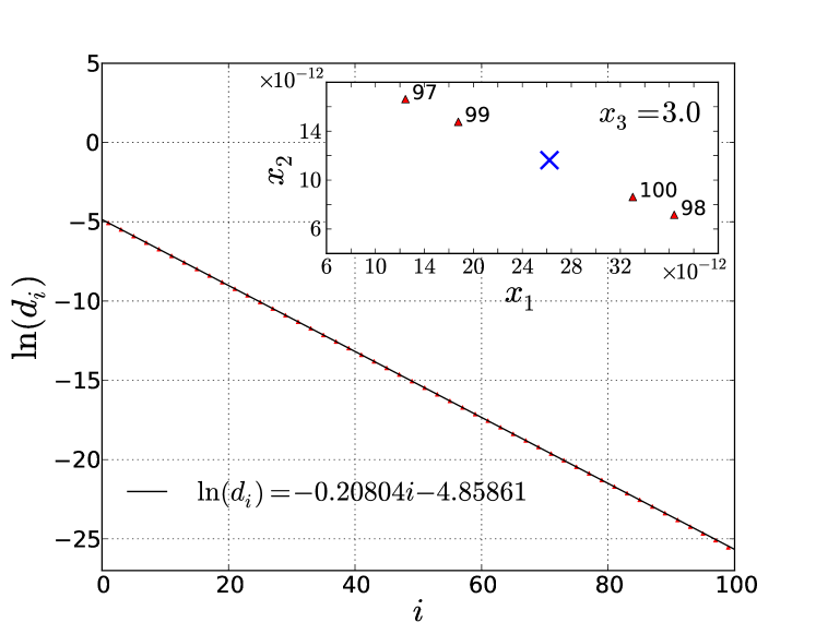
Figure 1: (Color online) Logarithmic plot of distance to convergence versus number of iterations, from the point on the orbit found by Zhou et al. zho01 , to the more accurate point found by the code in the Appendix after only 20 additional integration cycles. More than $100$ ordinary integration cycles are required before the Zhou et al. orbit converges to a distance smaller than $6\times 10^{-12}$. The inset shows a Poincaré section through the plane $x_{3}=3.0$, with successive intersections of the converging orbit indicated by (red) triangles, and the more accurate point by a (blue) cross. The bottom left corner of the inset correspond to $x_{1}=2.628655670296$ and $x_{2}=3.509456205164$. These values should be added to the corresponding axis labels.

point on the orbit, found by the optimized shooting method, has been plotted as a blue cross. The triangular markers in the inset show the successive crossing of the other orbit that slowly converges toward the cross. Note that labels for the horizontal and vertical axes of the inset should be multiplied by $10^{-12}$ and then added to $x_{1}=2.628655670296$ and $x_{2}=3.509456205164$, respectively. The last two coordinates are those of the bottom left corner of the inset.

As may be expected, the distances $d_{i}$ converge exponentially toward the stable limit cycle. The decay constant was found to be $-0.20804$. From the Poincaré section we see that it takes approximately an additional $100$ cycles before the orbit found by Zhou et al. zho01 converges to a distance of less than $6\times 10^{-12}$ away from the orbit found by the optimized shooting method. The same problem, namely the incomplete convergence of the orbit, is also responsible for inaccuracies in the results reported by Li and Xu li005 and it points to an important advantage of the present method. In the case of the code listed in Appendix A, convergence to the final orbit is complete after only $20$ integration cycles, as opposed to the more than $100$ additional cycles that are required before the other two methods converge to the true periodic orbit to the same accuracy. Moreover, in many applications one is interested in obtaining unstable periodic orbits, but numerical integration methods will fail to converge to unstable orbits. As we shall see in the next section, the optimized shooting method is also suitable for finding unstable periodic orbits.

To conclude this section we note that we have also tested and compared the new method for the case of period-2 and higher orbits. Figure 2 summarizes our results for the RS, by showing the phase portraits of the obtained period-1 and period-2 orbits.

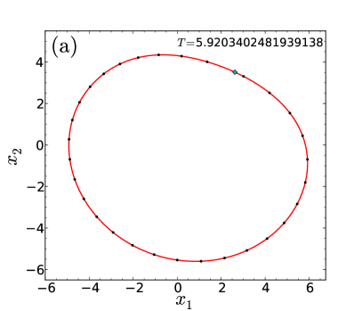
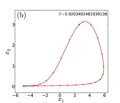
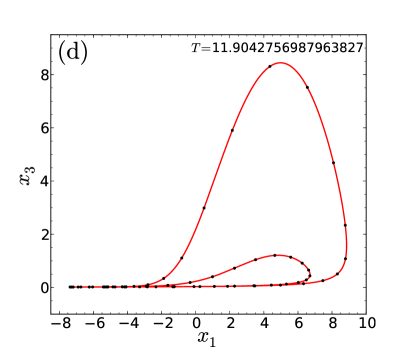
Figure 2: (Color online) Comparison of phase portraits obtained via the optimized shooting method, with that of Ref. li005 . Figures (a) and (b) show phase portraits of the period-1 solution obtained by solving Eq. (10) with $c=3.5$. Similarly. Figs. (c) and (d) show the period-2 solution, with $c=5.0$. The optimized periods are given in the upper right-hand corners of each figure. For Figs. (a) and (b), the precise coordinates of the point marked by (blue) diamond markers are listed in the first row of Table 1.

Figures 2(a) to (d) correspond very closely to to Figs. 1 to 4 in Ref. li005 . In the case of Figs. 2(c) and (d), for the parameter $c=5.0$, Li and Xu calculated the period of the bifurcated orbit to be $T=11.89692819$. From our calculated value, shown in upper right corner of Fig. 2(d), we see that the value that was calculated by Li and Xu li005 is again only accurate to two decimal places.

4 Unstable periodic orbits in the Rössler system

When applied to the RS the optimized shooting method finds, in addition to stable periodic orbits, a large number of unstable periodic orbits. In what follows we will characterize the stability of these orbits by calculating the characteristic (Floquet) multipliers, i.e. the eigenvalues of the monodromy matrix, according to the method developed by Lust lus01 . The monodromy matrix $\mathbf{M}\left(t\right)$ is the solution at time $T$ of the variational equation

$$\frac{d\mathbf{M}}{dt}=\mathbf{JM}\mbox{, \ \ with }\mathbf{M}\left(0\right)=\mathbf{1}\mbox{,}$$ (12)

where $\mathbf{J}$ is the system Jacobian. One of the Floquet multipliers, called the trivial multiplier, is always one. Its eigenvector is tangential to the limit cycle at the initial point $\mathbf{x}\left(0\right)$. A periodic solution is asymptotically stable if the modulus of each Floquet multiplier, except the trivial one, is strictly less than one. Otherwise, if one or more of the multipliers is greater than one in modulus, the solution is asymptotically unstable. For the stable orbits that were seen in Fig. 2, for example, the moduli of the largest nontrivial multipliers are found to be $\mu_{\max}=0.812252$ (in the case of Figs. 2(a) and (b)) and $\mu_{\max}=0.572052$ (in the case of Figs. 2(c) and (d)), respectively.

As a further test of the optimization method we have also optimized the parameters $a$, $b$ $c$ and $T$ in the Rössler system, for fixed initial values of the coordinates $(x_{1},x_{2},x_{3})$.

As the initial condition we systematically chose the coordinates to lie on three-dimensional cubic grids of varying sizes, starting from $8^{3}$ grid points, on a cube surrounding the origin of side length $1$, and systematically increasing the number of grid points and the cube length. In total, literally thousands of periodic orbits were thus obtained for the Rössler system by optimizing the four parameters. In some cases more than one periodic orbit (corresponding to different sets of optimized parameters) was found to pass through the initial condition. In most cases the found orbits were unstable. After examining several hundreds of these orbits graphically, we have concluded that they are qualitatively of two different types, depending on the sign of the $x_{3}$ coordinate.

To illustrate the main qualitative difference between the two types of orbits, we show four of the found orbits in Fig. 3. The orbits in Figs. 3(a) and (b) lie entirely in the half space $x_{3}>0$ and they all have a distinctive peak in the $x_{3}$ coordinate direction.

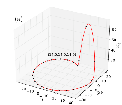
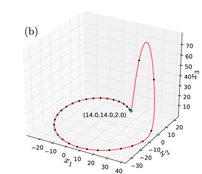
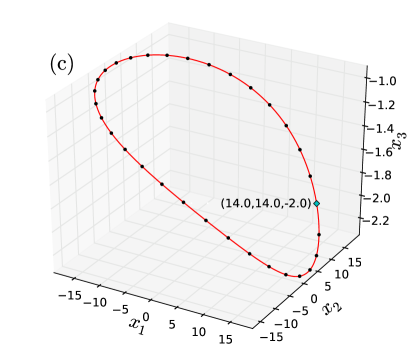
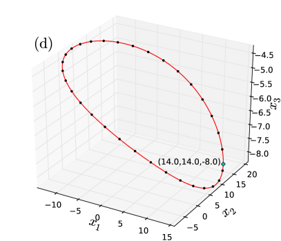
Figure 3: (Color online) Qualitative differences between periodic orbits of the Rössler system in the half space $x_{3}>0$, shown in (a) and (b), and in the half space $x_{3}<0$, shown in (c) and (d). Note the characteristic peak of the orbit in the $x_{3}$ direction, for $x_{3}>0$.

This peak is related to an exponential growth in the $x_{3}$ coordinate, when $x_{1}>0$. In this region the nonlinear term in the third equation of the RS tends to dominate, causing the exponential growth. However, depending on the value of the parameter $c$, as well as the other parameters in the system, the exponential growth in the coordinate $x_{3}$ eventually changes to exponential decay; either because the term $-cx_{3}$ becomes significant in comparison to the nonlinear term or else because of a change in sign of the coordinate $x_{1}$ (or both). Thus, qualitatively, all the obtained orbits for which $x_{3}>0$ were roughly elliptical, when projected onto the $x_{1}x_{2}$-plane, containing a characteristic peak in the $x_{3}$ direction, as show in Figs. 3(a) and (b). On the other hand, orbits for which $x_{3}<0$ were also elliptical in the $x_{1}x_{2}$-plane, but these did not have the exponential peak that was seen for the $x_{3}>0$ orbits. Two examples of orbits in the lower half plane are shown in Figs. 3(c) and (d). The optimized parameters for these orbits, together with the modulus of the largest non-trivial multiplier $\mu_{\max}$ and the magnitude of the located minimum in the residual $R_{\min}$ are listed in Table 2 for convenience. Each row in Table 2 is labeled by the corresponding figure number.

Fig.	$T$	$R_{\min}\left(10^{-13}\right)$	$\mu_{\max}$
3(a)	6.0368126768371511	6.07	5.635982
3(b)	6.1360301575904730	2.71	4.552192
3(c)	6.2906328270213132	0.08	1.037877
3(d)	6.3510302249381043	0.87	1.070770
Fig.	$a$	$b$	$c$
3(a)	0.2639519863856384	0.0076361389339972	28.4349476839393454
3(b)	0.2511744525989691	0.0681976088482620	29.4473072446435609
3(c)	-0.0360057068462920	-56.9446489079999978	42.8808270302575707
3(d)	-0.1323654753343560	-262.2015992062510463	46.9462750789147378

Table 2: Optimized periods $T$, minimum residuals $R_{\min}$ and the moduli of the largest non-trivial Floquet multipliers $\mu_{\max}$ corresponding to the the unstable periodic orbits shown in Fig. 3, for the optimized control parameters $a$, $b$ and $c$.

It is easy to see why closed orbits cannot cross the $x_{3}=0$ plane. If such orbits existed, they would have to cross the plane twice; once with $\dot{x}_{3}>0$ and once with $\dot{x}_{3}<0$. However, as Eq. (10) shows, for $x_{3}=0$ the sign of $\dot{x}_{3}$ is determined by the parameter $b$. Thus $\dot{x}_{3}$ can be either positive or negative, but its sign never alternates for a given set of parameters. If one does try to construct a periodic orbit passing through the plane $x_{3}=0$, the optimized shooting method simply fails to converge, indicating that the orbit does not exist.

To conclude this section we also investigate the degree of instability in the calculated unstable periodic orbits. The degree of instability is particularly important for unstable solutions with long periods (especially those embedded in strange attractors of a chaotic system). The latter problem is considered to be hard to solve and is therefore a good test of the present method.

For unstable orbits, numerical errors that occur during the integration procedure grow larger as the integration proceeds, and this growth eventually causes the trajectory to move away from the closed orbit. For the most unstable orbits which we have found, having $\mu_{\max}\approx 5$, such deviations become visible in the phase portraits after integration times of $15$-$20T$, where $T$ is the period of the shortest obtained (period-1) solution. In the least unstable cases, for which $\mu_{\max}$ is only slightly greater than one, the deviations become visible after about $80$-$100T$, i.e. after much longer integration times, as one would expect. It is also interesting to note that, after an unstable orbit has decayed, the trajectory may follow a variety of paths. In some cases we have found that it can decay into a quasi-periodic orbit (with essentially an infinite period), as shown in Figure 4(a), in other cases it can spiral inward or outward, either toward or away from a fixed point, as shown in Figs. 4(b) and (c), and lastly, it may enter the basin of attraction of the chaotic attractor, as shown in Fig. 4(d).

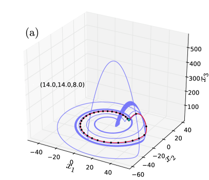
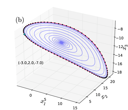
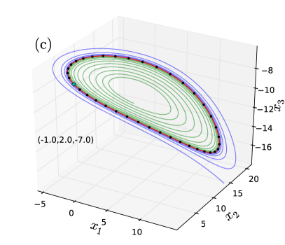
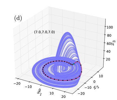
Figure 4: (Color online) Different types of paths followed by the unstable periodic orbits of the RS after they have decayed: (a) Quasi-periodic orbits, (b) and (c) Inward or outward spiral toward or away from a fixed point, and (d) Chaotic orbit in basin of attraction of a chaotic attractor. The blue and green lines spiraling out of and into the fixed point in (c) demonstrate the stochastic nature of the decay routes.

The precise parameter values corresponding to all the orbits shown in Fig. 4 are listed in Table 3 for convenience.

Fig.	$T$	$R_{\min}\left(10^{-13}\right)$	$\mu_{\max}$
4(a)	6.0692872165404559	0.57	5.301613
4(b)	7.6628544529751386	0.60	2.597276
4(c)	7.4670894888859385	0.23	1.844971
4(d)	6.0907519243177850	1.16	4.086460
Fig.	$a$	$b$	$c$
4(a)	0.2591659663922890	0.0157490292455600	28.9026881232841184
4(b)	-0.5160312363632790	-211.2660719529740447	27.0217872597939994
4(c)	-0.4931680147640250	-181.9747123841032987	24.8103827712413185
4(d)	0.2573147265532380	0.5728277554035760	13.6096389284738102

Table 3: Optimized periods $T$, minimum residuals $R_{\min}$ and the moduli of the largest non-trivial Floquet multipliers $\mu_{\max}$ corresponding to the unstable periodic orbits shown in Fig. 4, for the optimized control parameters $a$, $b$ and $c$.

We note that in Fig. 4(c), two spiral trajectories are shown: the first spiraling inward, the second outward. The difference seen here, in the way that this orbit decays, occurred as a result of using two different values for the integration time step. In the first case $\Delta\tau=1/1024$, and in the second $\Delta\tau=1/2048$. Thus it is clear that the small numerical errors that occur during the integration process can perturb the unstable trajectory in different ways. This observation emphasizes the stochastic nature of the decay routes that are depicted in Fig. 4.

5 Designing periodic orbits with specific characteristics

Unlike the other methods zho01 ; li005 , the optimized shooting method can be used to obtain periodic orbits with very specific characteristics. To illustrate this feature of the method, we consider the following hypothetical example.

Suppose we are interested in using a Field Programmable Gate Array (FPGA) implementation of the RS sad09 to generate a periodic electrical pulse of a particular amplitude (pulse height). We may select the coordinate $x_{3}$, for this purpose, and assume that the desired amplitude is $(x_{3})_{\max}=318.6$, in the dimensionless units of Eq. (11). The problem then is to optimize the parameters $a$, $b$, $c$, and $T$ (if indeed it is possible), in order to achieve the desired pulse.

To check the feasibility of this project one can use the optimization method to search for all stable periodic orbits for which the $x_{3}$ coordinate has the desired maximum. The only modification that needs to be made is to the definition of the residual. In addition to the components that were used previously (in Eq. (11)), extra components must be added to the residual in order to define the additional requirement for the maximum at $x_{3}=318.6$. Thus we must extend the definition of the residual to

$$\mathbf{R}=(\mathbf{x}\left(1\right)-\mathbf{x}\left(0\right),b+x_{3}\left(1\right)\left(x_{1}\left(1\right)-c\right),b+x_{3}\left(0\right)\left(x_{1}\left(0\right)-c\right))\,\mbox{,}$$ (13)

where the first three components are as before, and the last two components express the condition for the maximum, i.e. they come from the requirement $\dot{x}_{3}\left(1\right)=\dot{x}_{3}\left(0\right)=0$, with $x_{3}\left(0\right)=318.6$. The remaining two components of the initial condition, $x_{1}\left(0\right)$ and $x_{2}\left(0\right)$, can of course be chosen arbitrarily in order to set the phase of the pulse.

Figure 5(a) shows the optimized pulse obtained by using the modified residual (Eq. (13)), the initial condition $\left(-0.01,8.14,318.60\right)$ , and initial guess for the parameters: $a=-0.1,b=0,c=-0.1$, and $T=4$.

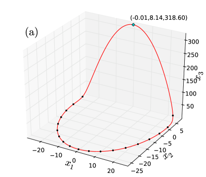
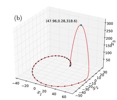
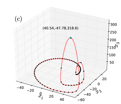
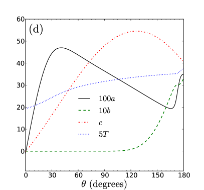
Figure 5: (Color online) Illustration of the usefulness of the property of the RS discovered in this work. The optimal parameters of the periodic orbit in (a) passing exactly through $\left(-0.01\mbox{, }8.14\mbox{, }318.60\right)$ are used in a subsequent optimization step of an orbit rotated from the previous one by $1$ degree relative to an axis parallel to the $x_{3}$-direction and passing through the point $\left(20,-20\right)$. (b) The orbit obtained after $90$ degrees of rotation. (c) After $180$ degrees of rotation. (d) The (scaled) optimized parameters as functions of the rotation angle.

In this case the optimized parameters for the pulse were found after $178$ iterations. In practice the question of how variations in the parameters will affect the phase of the pulse is also important.

To illustrate this more clearly we re-solve the same problem after rotating the initial coordinates $x_{1}(0)$ and $x_{2}(0)$ on a circle in the $x_{1}x_{2}$-plane. Starting from the initial condition $\left(-0.01,8.14,318.60\right)$ we rotate the initial condition by $1$ degree at a time about an axis parallel to the $x_{3}$-direction and passing through the point $\left(20,-20\right)$. For the optimization of the orbit through the rotated points we choose the the previously obtained optimized parameters as the initial guess.

Figure 5(b) shows the periodic orbit obtained after the first initial condition, i.e. $\left(-0.01\mbox{, }8.14\mbox{, }318.60\right)$, has been rotated clockwise by $90$ degrees about the axis of rotation. Similarly Fig. 5(c) shows the orbit after $180$ degrees of rotation. Figure 5(d) shows how the optimized system parameters may be varied continuously in order to achieve a smooth rotation in the phase of the pulse. In this example we have allowed the period $T$ of the pulse to vary while the phase is being rotated. However, there are many other possibilities afforded by the present method. For example, one can also rotate the phase of the pulse for a fixed period.

It is interesting to note that, as one perhaps may have anticipated, for the second and subsequent optimizations in the above example the number of iterations required to reach the set tolerance of $R_{\min}<10^{-14}$ become considerably fewer than the initial number of $178$. The subsequent optimizations only require $20$ to $35$ iterations to converge.

6 Periodic solutions of a coupled Rössler system

To test the optimization method on a system that exhibits high-dimensional chaos, we have also applied it to a six-dimensional (symmetrically) coupled RS ros96 , using for comparison the same parameter values that were considered in Ref. zho01 . The study of the dynamics of identical coupled nonlinear chaotic flows, such as two coupled RS ras96 ; yan01 ; pra13 , has provided insights into the chaotic behavior of higher dimensional systems. These systems exhibit hyperchaos, which differs from ordinary chaos in that there is more than one positive Lyapunov exponent, and hence more than one direction in phase space in which the chaotic attractor expands ras96 ; pra13 .

In the notation of Ref. zho01 , the system equations are given by

$$\dot{x}_{1} = -w_{1}x_{2}-x_{3}+c\left(x_{4}-x_{1}\right)$$

$$\dot{x}_{2} = w_{1}x_{1}+0.15x_{2}$$

$$\dot{x}_{3} = 0.2+x_{3}\left(x_{1}-3.5\right)$$ (14)

$$\dot{x}_{4} = -w_{2}x_{5}-x_{6}+c\left(x_{1}-x_{4}\right)$$

$$\dot{x}_{5} = w_{2}x_{4}+0.15x_{5}$$

$$\dot{x}_{6} = 0.2+x_{6}\left(x_{4}-3.5\right)$$

where $w_{1}=1.03$, $w_{2}=0.97$ and the coupling constant $c=0.13$.

To test our method on this six-dimensional system, we started from the initial condition $(1,0,1,0,1,0)$ and an initial guess, $T=5$, for the period.

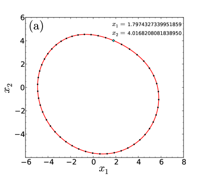
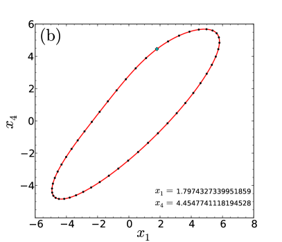
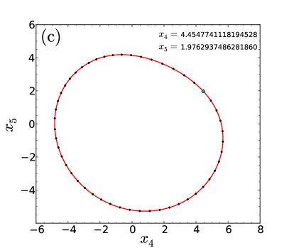
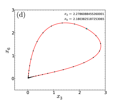
Figure 6: (Color online) Phase portraits of the periodic orbit found by the optimized shooting method, in agreement with the results of Ref. zho01 . The precise coordinates of one point on the orbit, indicated by a blue diamond marker, are listed in each figure.

The optimized period of $T=5.9773863584207021$ was found for the period-1 orbit, with an error in the residual $\sim 10^{-14}$. Figure 6 shows four projections of the phase portrait for the calculated periodic orbit, together with one point on the orbit. Figures 6(a)-(c) are the same as Figs. 2-4 in the paper by Zhou et al. zho01 The magnitude of the largest non-trivial Floquet multiplier for this orbit was found to be $\mu_{\max}=0.649768$, indicating that the orbit is stable. For other values of the control parameters the system was found to exhibit quasi-periodic behaviour, interrupted by periodic windows in which frequency-locking occurs, in agreement with Ref. ras96 .

7 Periodic solution of a flexible rotor-bearing system

To demonstrate that our method is equally applicable to non-autonomous systems, we model the Jeffcott flexible rotor-bearing system that was tested by Li and Xu li005 . This non-autonomous system also exhibits high-dimensional chaos. In the notation of Ref. li005 , the system equation is given by

$$\dot{x}_{i} = x_{i+4}\mbox{ \ \ (}i=1,2,3,4\mbox{) }$$

$$\dot{x}_{5} = -\frac{\sigma}{\omega}f_{x}+\frac{d}{\omega}\left(x_{7}-x_{5}\right)+\frac{k}{\omega^{2}}\left(x_{3}-x_{1}\right)$$

$$\dot{x}_{6} = -\frac{\sigma}{\omega}f_{y}+\frac{d}{\omega}\left(x_{8}-x_{6}\right)+\frac{k}{\omega^{2}}\left(x_{4}-x_{2}\right)-\frac{1}{\omega^{2}}$$ (15)

$$\dot{x}_{7} = \beta\cos\tau+\frac{d}{\gamma\omega}\left(x_{5}-x_{7}\right)+\frac{k}{\gamma\omega^{2}}\left(x_{1}-x_{3}\right)$$

$$\dot{x}_{8} = \beta\sin\tau+\frac{d}{\gamma\omega}\left(x_{6}-x_{8}\right)+\frac{k}{\gamma\omega^{2}}\left(x_{2}-x_{4}\right)-\frac{1}{\omega^{2}}$$

where $\sigma=0.843$, $k=5893.9$, $d=7.677$, $\gamma=16$, $\beta=0.14328$ and $\omega$ is the variable parameter which is related to the angular frequency at which the rotor is driven. In the last equation the overdot indicates the total time derivative with respect to the dimensionless time $\tau$ and the components of the nonlinear oil film force are

$$f_{x}=-p_{r}\cos\psi-p_{t}\sin\psi\mbox{ and \ }f_{y}=-p_{r}\sin\psi+p_{t}\cos\psi\mbox{, }$$ (16)

where

$$p_{r} = \frac{6\varepsilon^{2}(1-2\dot{\psi})}{(1-\varepsilon^{2})(2+\varepsilon^{2})}+\frac{3\dot{\varepsilon}}{(1-\varepsilon^{2})^{3/2}}\left(\pi-\frac{16}{\pi(2+\varepsilon^{2})}\right)\mbox{ and}$$

$$p_{t} = \frac{3\pi\varepsilon(1-2\dot{\psi})}{(1-\varepsilon^{2})^{1/2}(2+\varepsilon^{2})}+\frac{12\varepsilon\dot{\varepsilon}}{(1-\varepsilon^{2})(2+\varepsilon^{2})}$$

are the radial and tangential forces on the oil film. (See Refs. cho13 ; sha90 for details.) We note here that it was extremely difficult to reconstruct the full set of equations from the information provided in the paper by Li and Xu li005 , firstly because of two typographical errors in their equations, and secondly because their equations were incomplete, with the only references provided to unavailable papers in Chinese. In view of these difficulties we have corrected the typographical errors and provided (with the help of Refs. cho13 ; sha90 and the references therein) the missing transformation equations,

$$x_{1}=-\varepsilon\cos\psi\mbox{ and \ }x_{2}=-\varepsilon\sin\psi\mbox{, }$$ (17)

that allow one to express the polar coordinates, $\varepsilon$ and $\psi$, and their total time derivatives, in terms of the dynamical variables $x_{1}$ and $x_{2}$.

Figure 7 shows good agreement for the quantities that were

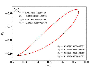
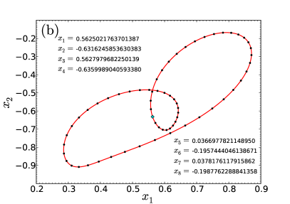
Figure 7: (Color online) Phase portraits reproduced from Ref. li005 for the Jeffcott rotor-bearing system by the numerical method described in this paper. (a) The period-1 solution of Eq. (15) obtained from the initial conditions shown when $\omega=1.2$. (b) The period-2 solution obtained when $\omega=2.3$ and the starting conditions shown are used.

plotted in Figs. 6 and 7 of Ref. li005 . Starting from the same initial conditions that were used in Ref. li005 , we calculated the period of the period-1 orbit ($\omega=1.2$) to be $T=6.2831853071795498$. The phase portrait for the corresponding orbit is shown in Fig. 7(a), together with the coordinates of one point on the orbit. For the period-2 orbit ($\omega=2.3$), shown in Fig. 7(b), our method produces an optimized period of $T=12.5663706143591707$. The calculated periods agree with the theoretically expected values of $2\pi$ ($4\pi$) to an impressive thirteen (fourteen) decimal places.

8 Conclusion

We have developed an optimized shooting method for finding the periodic solutions of both autonomous and non-autonomous nonlinear systems of differential equations. The method essentially re-casts the problem of finding periodic orbits in a form that is suitable for applying multi-dimensional optimization. In the present work we have made use of Levenberg-Marquardt optimization (LMO) for this purpose. LMO is widely regarded as being one of the most efficient methods of optimization for medium-sized problems, i.e. for those with up to a few hundred weights.

Since LMO is already available in the standard libraries for the most important scientific programming languages, such as Python, Fortran, Matlab, C and C++, our present method for finding periodic orbits is relatively easy to implement and does not require additional resources. In the present work we have provided a simple implementation of the method in the Python programming language. Even though we have only explored a few possible ways of defining the residual (error vector) that is required for the method, we would like to emphasize that the true versatility of the method ultimately depends on the user’s ability to define the residual appropriately. Nevertheless we hope that the present examples have served to illustrate the basic idea behind the method and that they will in future stimulate the creative use of the optimized shooting method for finding periodic orbits in nonlinear dynamical systems.

Appendix A: Example of computer implementation

The following code, written in the Python programming language chu07 , sets up and minimizes the residual vector $\mathbf{R}$, given by Eq. (11), excluding the $x_{3}$-coordinate from the minimization. Although there is an integration scheme which is specially adapted to orbital problems such as these ana05 , the present example makes use of a fifth-order Runge-Kutta scheme that already produces excellent results. In the code below the function f() returns the derivatives for the Rössler system. The function ef() returns the residual by integrating the system from $\tau=0$ to $\tau=1+p\Delta\tau$, through calls to integrate(). In the present example, $p=2$, and the step size is set to $\Delta\tau=1/1024$. The code given below is designed to work with step sizes of the form $1/2^{\ell}$, where $\ell$ is an appropriately chosen positive integer. The function leastsq(), which is imported from the module scipy.optimize lan04 , uses LMO to minimize the residual defined in the function ef(). The function leastsq() is called from within the main() function, which sets up the initial parameters and quantities to be optimized. Notice that in this example, only the three quantities $x_{1}$, $x_{2}$ and $T$ are passed to leastsq() for optimization, via the vector v0.

from scipy import zeros, concatenate, sqrt, dot
from scipy.optimize import leastsq

def f(t,x,T,a):
    """
    Rossler system written in the form of Eq. (7)
    """
    xd = zeros(len(x),’d’)
    xd[0] = T*(-x[1]-x[2])
    xd[1] = T*(x[0]+a[0]*x[1])
    xd[2] = T*(a[1]+x[2]*x[0]-a[2]*x[2])
    return xd

def integrate(t,x,func,h,w,a):
    """
    5th-order Runge-Kutta integration scheme. Input:
    t - initial time
    x - vector of initial conditions at initial time t
    h - integration time step, w - period
    a - additional parameters
    """
    k1=h*func(t,x,w,a)
    k2=h*func(t+0.5*h,x+0.5*k1,w,a)
    k3=h*func(t+0.5*h,x+(3.0*k1+k2)/16.0,w,a)
    k4=h*func(t+h,x+0.5*k3,w,a)
    k5=h*func(t+h,x+(-3.0*k2+6.0*k3+9.0*k4)/16.0,w,a)
    k6=h*func(t+h,x+(k1+4.0*k2+6.0*k3-12.0*k4+8.0*k5)/7.0,w,a)
    xp = x + (7.0*k1+32.0*k3+12.0*k4+32.0*k5+7.0*k6)/90.0
    return xp

def ef(v,x,func,dt,a,p):
    """
    Residual (error vector). Input:
    v - vector containing the quantities to be optimized
    x - vector of initial conditions
    func - function, dt - integration time step
    a - additional parameters
    p - controls length of error vector
    """
    j = int(2.0/dt)
    vv = zeros((j,len(x)),’d’)
    vv[0,0:2] = v[0:2]       # set initial condition
    vv[0,2] = x[2]
    T = v[2]                 # set period
    i = 0
    while i < j/2+p:
        t = i*dt
        vv[i+1,:] = integrate(t,vv[i,:],func,dt,T,a)
        i = i+1
    er = vv[j/2,:]-vv[0,:]   # creates residual error vector
    for i in range(1,p):     # of appropriate length
        er = concatenate((er,vv[j/2+i,:]-vv[i,:]))
    print ’Error:’, sqrt(dot(er,er))
    return er

def main():
    a0 = zeros(3,’d’)        # predetermined system parameters
    a0[0] = 0.15; a0[1] = 0.2; a0[2] = 3.5
    x0 = zeros(3,’d’)        # initial conditions (N=3)
    x0[0] = 2.7002161609; x0[1] = 3.4723025491; x0[2] = 3.0
    v0 = zeros(3,’d’)        # quantities for optimization
    v0[0:2] = x0[0:2]
    v0[2] =   5.92030065     # initial guess for period
    p = 2                    # length of residual is pN
    h = 1.0/1024.0           # integration time step
    #                        # LM optimization
    v, succ = leastsq(ef,v0,args=(x0,f,h,a0,p),ftol=1e-12,maxfev=200)
    err = ef(v,x0,f,h,a0,p)  # error estimation
    es = sqrt(dot(err,err))
    #
    fout = open(’fig1ab.dat’,’w’) # for file output
    u0 = (v[0],v[1],x0[2],v[2],es/1e-13)
    print (’%20.16f %20.16f %20.16f %20.16f %6.2f’ % u0)
    print >> fout,(’%20.16f %20.16f %20.16f %20.16f %6.2f’ % u0)
    fout.close()

main()

The above code executes in 3.78 CPU seconds on an Intel 3.0 GHz Xeon processor and requires a maximum memory (RAM) of 2MB, with at least 30MB of additional swap space. The output of the code is written to screen as well as to the file called fig1ab.dat. After execution the file will contain the following numbers:

2.6286556703142154 3.5094562051716300 3.0000000000000000
5.9203402481939138 0.21

Here the quantities are: the optimized initial point on the periodic orbit, the corresponding period, and the magnitude of the final value of the residual, divided by $10^{-13}$.

References

- (1) Z. Galias, Int. J. Bifurcation Chaos 11, 2427 (2001)
- (2) R.C. Hilborn, Chaos and Nonlinear Dynamics: An Introduction, pp. 413-414, 2nd edn. (Oxford University Press, New York, 2000)
- (3) P.H. Franses, D. van Dijk, Nonlinear Time Series Models in Empirical Finance (Cambridge University Press, Cambridge, 2000)
- (4) J. Guckenheimer, B. Meloon, SIAM J. Sci. Comput. 22, 951 (2000)
- (5) P. Deuflhard, in Computational Techniques for Ordinary Differential Equations, ed. by I. Gladwell, D.K. Sayers (Academic Press, New York, 1980), p. 217
- (6) U. Ascher, R. Mattheij, R. Russell, Numerical Solution of Boundary Value Problems (Prentice Hall, Englewood Cliffs, NJ, 1988)
- (7) T. Zhou, J.X. Xu, C.L. Chen, J. Sound Vib. 245, 239 (2001)
- (8) O.E. Rössler, Phys. Lett. A 57, 397 (1976)
- (9) M.G. Rosenblum, A.S. Pikovsk, J. Kurths, Phys. Rev. Lett. 76, 1804 (1996)
- (10) D. Li, J. Xu, Engineering with Computers 20, 316 (2005)
- (11) M. Chouchane, R. Sghir, in MEDYNA 2013: 1st Euro-Mediterranean Conference on Structural Dynamics and Vibroacoustics (Marrakech, Morocco, 2013), pp. 1–4
- (12) J. Shaw, S. Shaw, Nonlinear Dynamics 1, 293 (1990)
- (13) K. Levenberg, Quart. Appl. Math. 2, 164 (1944)
- (14) D.W. Marquardt, SIAM J. Appl. Math. 11, 431 (1963)
- (15) J. Fan, Mathematics of Computation 81, 447 (2012)
- (16) J. Fan, J. Zeng, Appl. Math. Comput. 219, 9438 (2013)
- (17) S. Roweis, Levenberg-Marquardt Optimization. Tech. rep., Available online at http://www.cs.nyu.edu/~roweis/notes/lm.pdf (2013)
- (18) J.W. Kim, P.A. Robinson, Phys. Rev. E 75, 031907 (2007)
- (19) H. Gavin, The Levenberg-Marquardt method for nonlinear least squares curve-fitting problems. Tech. rep., Duke University (2011)
- (20) M. Gilli, D. Maringer, E. Schumann, Numerical Methods and Optimization in Finance (Academic Press, Waltham, MA, USA, 2011)
- (21) H.P. Langtangen, Python Scripting for Computational Science, 3rd edn. (Springer Verlag, Berlin, 2008)
- (22) K. Lust, Int. J. Bifurcation Chaos 11, 2389 (2001)
- (23) S. Sadoudi, M.S. Azzaz, in Proceedings of the 5th International Conference: Sciences of Electronic,Technologies of Information and Telecommunications (22-26 March, 2009)
- (24) J. Rasmussen, E. Mosekilde, C. Reick, Mathematics and Computers in Simulation 40, 247 (1996)
- (25) S. Yanchuk, Y. Maistrenko, E. Mosekilde, Physica D 154, 26 (2001)
- (26) W. Prants, P. Rech, Physica Scripta 88, 015001 (2013)
- (27) W.J. Chun, Core Python Programming, 2nd edn. (Prentice Hall, New Jersey, 2007)
- (28) Z.A. Anastassi, T.E. Simos, J. Comput. Appl. Math. 175, 1 (2005)