Second Order Differences of Cyclic Data
and Applications in Variational Denoising

Abstract

In many image and signal processing applications, as interferometric synthetic aperture radar (SAR) or color image restoration in HSV or LCh spaces the data has its range on the one-dimensional sphere $\mathbb{S}^{1}$. Although the minimization of total variation (TV) regularized functionals is among the most popular methods for edge-preserving image restoration such methods were only very recently applied to cyclic structures. However, as for Euclidean data, TV regularized variational methods suffer from the so called staircasing effect. This effect can be avoided by involving higher order derivatives into the functional.

This is the first paper which uses higher order differences of cyclic data in regularization terms of energy functionals for image restoration. We introduce absolute higher order differences for $\mathbb{S}^{1}$-valued data in a sound way which is independent of the chosen representation system on the circle. Our absolute cyclic first order difference is just the geodesic distance between points. Similar to the geodesic distances the absolute cyclic second order differences have only values in $[0,\pi]$. We update the cyclic variational TV approach by our new cyclic second order differences. To minimize the corresponding functional we apply a cyclic proximal point method which was recently successfully proposed for Hadamard manifolds. Choosing appropriate cycles this algorithm can be implemented in an efficient way. The main steps require the evaluation of proximal mappings of our cyclic differences for which we provide analytical expressions. Under certain conditions we prove the convergence of our algorithm. Various numerical examples with artificial as well as real-world data demonstrate the advantageous performance of our algorithm.

1 Introduction

A frequently used method for edge-preserving image denoising is the variational approach which minimizes the Rudin-Osher-Fatemi (ROF) functional [40]. In a discrete (penalized) form the ROF functional can be written as

$$\sum_{i,j}(f_{i,j}-x_{i,j})^{2}+\lambda\sum_{i,j}\lvert\nabla x_{i,j}\rvert,\quad\lambda>0,$$

where $f\in\mathbb{R}^{N,M}$ is the given corrupted image and $\nabla$ denotes the discrete gradient operator which contains usually first order forward differences in vertical and horizontal directions. The regularizing term $\sum_{i,j}\lvert\nabla x_{i,j}\rvert$ can be considered as discrete version of the total variation (TV) functional. Since the gradient does not penalize constant areas the minimizer of the ROF functional tends to have such regions, an effect known as staircasing. An approach to avoid this effect consists in the employment of higher order differences/derivatives. Since the pioneering work [10] which couples the TV term with higher order terms by infimal convolution various techniques with higher order differences/derivatives were proposed in the literature, among them [8, 11, 12, 15, 16, 27, 29, 31, 32, 41, 42, 43].

In various applications in image processing and computer vision the functions of interest take values on the circle $\mathbb{S}^{1}$ or another manifold. Processing manifold-valued data has gained a lot of interest in recent years. Examples are wavelet-type multiscale transforms for manifold data  [25, 37, 49] and manifold-valued partial differential equations  [13, 24]. Finally we like to mention statistical issues on Riemannian manifolds [19, 20, 36] and in particular the statistics of circular data [18, 28]. The TV notation for functions with values on a manifold has been studied in [22, 23] using the theory of Cartesian currents. These papers were an extension of the previous work [21] were the authors focus on $\mathbb{S}^{1}$-valued functions and show in particular the existence of minimizers of certain energies in the space of functions with bounded total cyclic variation. The first work which applies a cyclic TV approach among other models for imaging tasks was recently published by Cremers and Strekalovskiy in [44, 45]. The authors unwrapped the function values to the real axis and proposed an algorithmic solution to account for the periodicity. An algorithm which solves TV regularized minimization problems on Riemannian manifolds was proposed by Lellmann et al. in [30]. They reformulate the problem as a multilabel optimization problem with an infinite number of labels and approximate the resulting hard optimization problem using convex relaxation techniques. The algorithm was applied for chromaticity-brightness denoising, denoising of rotation data and processing of normal fields for visualization. Another approach to TV minimization for manifold-valued data via cyclic and parallel proximal point algorithms was proposed by one of the authors and his colleagues in [50]. It does not require any labeling or relaxation techniques. The authors apply their algorithm in particular for diffusion tensor imaging and interferometric SAR imaging. For Cartan-Hadamard manifolds convergence of the algorithm was shown based on a recent result of Bačák [1]. Unfortunately, one of the simplest manifolds that is not of Cartan-Hadamard type is the circle $\mathbb{S}^{1}$.

In this paper we deal with the incorporation of higher order differences into the energy functionals to improve denoising results for $\mathbb{S}^{1}$-valued data. Note that the (second-order) total generalized variation was generalized for tensor fields in [46]. However, to the best of our knowledge this is the first paper which defines second order differences of cyclic data and uses them in regularization terms of energy functionals for image restoration. We focus on a discrete setting. First we provide a meaningful definition of higher order differences for cyclic data which we call absolute cyclic differences. In particular our absolute cyclic first order differences resemble the geodesic distance (arc length distance) on the circle. As the geodesics the absolute cyclic second order differences take only values in $[0,\pi]$. This is not necessary the case for differences of order larger than two. Following the idea in [50] we suggest a cyclic proximal point algorithm to minimize the resulting functionals. This algorithm requires the evaluation of certain proximal mappings. We provide analytical expression for these mappings. Further, we suggest an appropriate choice of the cycles such that the whole algorithm becomes very efficient. We apply our algorithm to artificial data as well as to real-world interferometric SAR data.

The paper is organized as follows: in Section 2 we propose a definition of differences on $\mathbb{S}^{1}$. Then, in Section 3, we provide analytical expressions for the proximal mappings required in our cyclic proximal point algorithm. The approach is based on unwrapping the circle to $\mathbb{R}$ and considering the corresponding proximal mappings on the Euclidean space. The cyclic proximal point algorithm is presented in Section 4. In particular we describe a vectorization strategy which makes the Matlab implementation efficient and provides parallelizability, and prove its convergence under certain assumptions. Section 5 demonstrates the advantageous performance of our algorithm by numerical examples. Finally, conclusions and directions of future work are given in Section 6.

2 Differences of $\mathbb{S}^{1}$–valued data

Let $\mathbb{S}^{1}$ be the unit circle in the plane

$$\mathbb{S}^{1}:=\{p_{1}^{2}+p_{2}^{2}=1:p=(p_{1},p_{2})^{\mathrm{T}}\in\mathbb{R}^{2}\}$$

endowed with the geodesic distance (arc length distance)

$$d_{\mathbb{S}^{1}}(p,q)=\arccos(\langle p,q\rangle).$$

Given a base point $q\in\mathbb{S}^{1}$, the exponential map  $\exp_{q}:\mathbb{R}\rightarrow\mathbb{S}^{1}$ from the tangent space $T_{q}\mathbb{S}^{1}\simeq\mathbb{R}$ of $\mathbb{S}^{1}$ at $q$ onto $\mathbb{S}^{1}$ is defined by

$$\exp_{q}(x)=R_{x}q,\qquad R_{x}:=\begin{pmatrix}\cos x&-\sin x\\ \sin x&\cos x\end{pmatrix}.$$

This map is $2\pi$-periodic, i.e., $\exp_{q}(x)=\exp_{q}((x)_{2\pi})$ for any $x\in\mathbb{R}$, where $(x)_{2\pi}$ denotes the unique point in $[-\pi,\pi)$ such that $x=2\pi k+(x)_{2\pi}$, $k\in\mathbb{Z}$. Some useful properties of the mapping  $(\cdot)_{2\pi}:\mathbb{R}\rightarrow[-\pi,\pi)$ (which can also be considered as mapping from $\mathbb{R}$ onto $\mathbb{R}/2\pi\mathbb{Z}$) are collected in the following remark.

Remark 2.1.

The following relations hold true:

1. $\big{(}(x)_{2\pi}\pm(y)_{2\pi}\big{)}_{2\pi}=(x\pm y)_{2\pi}\qquad$ for all $x,y\in\mathbb{R}$.

2. If $z=(x-y)_{2\pi}$ then $x=(z+y)_{2\pi}\qquad$ for all $x\in[-\pi,\pi),\ y\in\mathbb{R}$.

While i) follows by straightforward computation relation ii) can be seen as follows: For $z=(x-y)_{2\pi}$ there exists $k\in\mathbb{Z}$ such that

$$x-y=(x-y)_{2\pi}+2\pi k=z+2\pi k.$$

Hence it follows $x=z+y+2\pi k$ and since $x\in[-\pi,\pi)$ further

$$x=(x)_{2\pi}=(z+y+2\pi k)_{2\pi}=(z+y)_{2\pi}.$$

To guarantee the injectivity of the exponential map, we restrict its domain of definition from $\mathbb{R}$ to $[-\pi,\pi)$. Thus, for $p,q\in\mathbb{S}^{1}$, there is now a unique $x\in[-\pi,\pi)$ satisfying $\exp_{q}(x)=p$. In particular we have $\exp_{q}(0)=q$. Given such representation system $x_{j}\in[-\pi,\pi)$ of $p_{j}\in\mathbb{S}^{1}$, $j=1,2$ centered at an arbitrary point $q$ on $\mathbb{S}^{1}$ the geodesic distance becomes

$$d_{\mathbb{S}^{1}}(p_{1},p_{2})=d(x_{1},x_{2})=\min_{k\in\mathbb{Z}}\lvert x_{2}-x_{1}+2\pi k\rvert=\lvert(x_{2}-x_{1})_{2\pi}\rvert.$$ (1)

Actually we need only $k\in\{0,\pm 1\}$ in the minimum. Clearly, this definition does not depend on the chosen center point $q$.

We want to determine general finite differences of $\mathbb{S}^{1}$-valued data. Let $w=(w_{j})_{j=1}^{d}\in\mathbb{R}^{d}\backslash\{0\}$ with

$$\langle w,1_{d}\rangle=\sum_{j=1}^{d}w_{j}=0,$$ (2)

where $1_{d}$ denotes the vector with $n$ components one. We define the finite difference operator $\Delta(\cdot;w):\mathbb{R}^{d}\rightarrow\mathbb{R}$ by

$$\Delta(x;w):=\langle x,w\rangle\quad\mbox{for all}\;x\in\mathbb{R}^{d}.$$

By (2), we see that $\Delta(\cdot;w)$ vanishes for constant vectors and is therefore translation invariant, i.e.,

$$\Delta(x+\alpha 1_{d};w)=\Delta(x;w)\quad\mbox{for all}\;\alpha\in\mathbb{R}.$$ (3)

Example 2.2.

For the binomial coefficients with alternating signs

$$w=b_{n}:=\left((-1)^{j+n-1}{n\choose{j-1}}\right)_{j=1}^{n+1}$$

we obtain the (forward) differences of order $n$:

$$\Delta(x;w)=\Delta_{n}(x)=\langle x,b_{n}\rangle=\sum_{j=1}^{n+1}(-1)^{j+n-1}{n\choose{j-1}}x_{j}.$$

Note that $\Delta_{n}$ does not only fulfill (2), but vanishes exactly for all ‘discrete polynomials of order $n-1$’, i.e., for all vectors from $\operatorname{span}\{(j^{r})_{j=0}^{n}:r=0,\ldots,n-1\}$. Here we are interested in first and second order differences

$$\Delta_{1}(x_{1},x_{2}) =\Delta(x;b_{1})=x_{2}-x_{1},$$

$$\Delta_{2}(x_{1},x_{2},x_{3}) =\Delta(x;b_{2})=x_{1}-2x_{2}+x_{3}.$$

Moreover, we will apply the ‘mixed second order’ difference with $w=b_{1,1}:=(-1,1,1,-1)^{\mathrm{T}}$ and use the notation

$$\Delta_{1,1}(x_{1},x_{2},x_{3},x_{4})=\Delta(x;b_{1,1})=-x_{1}+x_{2}+x_{3}-x_{4}.$$

We want to define differences for points $(p_{j})_{j=1}^{d}\in(\mathbb{S}^{1})^{d}$ using their representation $x:=(x_{j})_{j=1}^{d}\in[-\pi,\pi)^{d}$ with respect to an arbitrary fixed center point. As the geodesic distance (1) these differences should be independent of the choice of the center point. This can be achieved if and only if the differences are shift invariant modulo $2\pi$. Let $\mathbb{I}_{d}:=\{1,\ldots,d\}$. We define the absolute cyclic difference of $x\in[-\pi,\pi)^{d}$ (resp. $(p_{j})_{j=1}^{d}\in(\mathbb{S}^{1})^{d}$) with respect to $w$ by

$$d(x;w):=\min_{\alpha\in\mathbb{R}}\bigl{\lvert}\Delta\big{(}[x+\alpha 1_{d}]_{2\pi};w\big{)}\bigr{\rvert}=\min_{j\in\mathbb{I}_{d}}\bigl{\lvert}\Delta\big{(}[x-(x_{j}+\pi)1_{d}]_{2\pi};w\big{)}\bigr{\rvert},$$ (4)

where $[x]_{2\pi}$ denotes the component-by-component application of $(t)_{2\pi}$ if $t\not=(2k+1)\pi$, $k\in\mathbb{Z}$ and $[(2k+1)\pi]_{2\pi}=\pm\pi$, $k\in\mathbb{Z}$. The definition allows that points having the same value are treated separately, cf. Figure 2. This ensures that $d(\cdot;w):(\mathbb{S}^{1})^{d}\rightarrow\mathbb{R}$ is a continuous map. For example we have $d\bigl{(}(-\pi,0,-\pi)^{\mathrm{T}};b_{2}\bigr{)}=0$. Figures 1 and 2 illustrate definition (4). For the absolute cyclic differences related to the differences in Example 2.2 we will use the simpler notation

$$d_{n}(x):=d(x;b_{n})\quad\text{and}\quad d_{1,1}(x):=d(x;b_{1,1}).$$ (5)

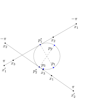
 (a) ${\exp}_{p_{1}^{*}}$ (top) and ${\exp}_{p_{2}^{*}}$ (bottom).

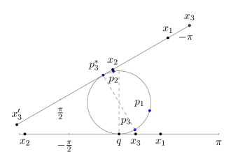
 (b) ${\exp}_{p_{3}^{*}}$ (top) and ${\exp}_{q}$ (bottom).

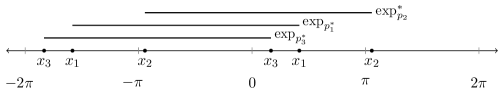
 (c) Settings from the tangential maps of $p_{j}^{*}$, $j=1,2,3$, on $\mathbb{R}$ using the representation system according to $\exp_{q}$.

Figure 1: Three points $p_{j}$, $j=1,2,3$, on the circle (blue) and their inverse exponential maps at $p_{j}^{*}$, $j=1,2,3$, (dark blue), where $p_{j}^{*}$ denotes the antipodal point of $p_{j}$. In other words, we cut the circle at the point $p_{j}$ and unwind it with respect to the tangent line at the antipodal point $p_{j}^{*}$. The absolute cyclic differences take the three pairwise different positions of the points $x_{j}$, $j=1,2,3$ to each other into account. These are shown in1 (c) with respect to the representation system from the arbitrary point $q$ in1 (b).

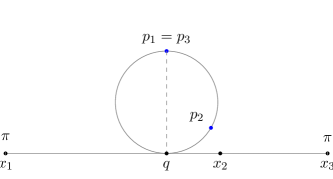
Figure 2: Three points $p_{j}$, $j=1,2,3$ on the circle, where $p_{1}=p_{3}$ and ${\exp}_{q}$, $q=p_{1}^{*}$. Though $p_{1},p_{3}$ denote the same point on the circle they are treated separately in the definition of the absolute cyclic differences.

The following equivalent definition of absolute cyclic differences appears to be useful.

Lemma 2.3.

Let $x\in[-\pi,\pi)^{d}$ be sorted in ascending order as $-\pi\leq x_{j_{1}}\leq\ldots\leq x_{j_{d}}<\pi$ and set $x^{1}:=(x_{j_{i}})_{i=1}^{d}$. Let $P$ denote the corresponding permutation matrix, i.e., $Px=x^{1}$ and $x=P^{\mathrm{T}}x^{1}.$ Consider the $2\pi$ shifted versions of $x^{1}$ given by

$$x^{k}=x^{1}+2\pi\sum_{j=1}^{k-1}e_{j}\quad k=2,\ldots,d,$$

where $e_{j}\in\mathbb{R}^{d}$ denotes the $j$-th unit vector. Then it holds

$$d(x;w)=\min_{k\in\mathbb{I}_{d}}\bigl{\lvert}\Delta(P^{\mathrm{T}}x^{k};w)\bigr{\rvert}=\min_{k\in\mathbb{I}_{n}}\Bigl{\lvert}\Delta(x^{k};w)+2\pi\Bigl{\langle}\sum_{j=1}^{k-1}e_{j},Pw\Bigr{\rangle}\Bigr{\rvert}.$$ (6)

Proof.

The first equality in (6) follows directly by definition (4). To see the second one, note that by linearity of the inner product we have

$$\langle P^{\mathrm{T}}x^{k},w\rangle=\langle P^{\mathrm{T}}x^{1},w\rangle+2\pi\Bigl{\langle}\sum_{j=1}^{k-1}e_{j},Pw\Bigr{\rangle}=\langle x,w\rangle+2\pi\Bigl{\langle}\sum_{j=1}^{k-1}e_{j},Pw\Bigr{\rangle}.$$ (7)

∎

For the geodesic distance we obtain by (1) that $d_{1}(x)=\big{\lvert}\big{(}\Delta_{1}(x))_{2\pi}\big{)}\big{\rvert}$. In general the relation

$$d(x;w)=\lvert(\langle x,w\rangle)_{2\pi}\rvert\qquad\text{ for all }x\in[-\pi,\pi)^{d}$$ (8)

does not hold true as the following example shows.

Example 2.4.

In general the $n$-th order absolute cyclic difference cannot be written as $d_{n}(x)=\lvert(\langle x,b_{n}\rangle)_{2\pi}\rvert=\lvert(\Delta_{n}(x))_{2\pi})\rvert.$ Consider for example the absolute cyclic third order difference for $x:=\frac{\pi}{16}(-15,-13,12,14)^{\mathrm{T}}$ given by (6) as

$$d_{3}(x_{1},x_{2},x_{3},x_{4})=\min_{k=1,2,3,4}\Delta_{3}(x^{k}),\quad\Delta_{3}(x)=-x_{1}+3x_{2}-3x_{3}+x_{4}.$$

We obtain

$$\Delta_{3}(x^{1})=\Delta_{3}(x)=\frac{-46\pi}{16},\;\Delta_{3}(x^{2})=\Delta_{3}(x^{4})=\frac{-78\pi}{16},\;\Delta_{3}(x^{3})=\frac{18\pi}{16},$$

so that $d_{3}(x)=\frac{18\pi}{16}>\pi$.

For $w\in\{b_{2},b_{1,1}\}$ relation  (8) holds true by the next lemma.

Proposition 2.5.

For $w\in\{b_{2},b_{1,1}\}$ the following relation holds true:

$$d(x;w)=\min_{k\in\mathbb{Z}}\lvert\Delta(x;w)+2\pi k\rvert=\bigl{\lvert}\bigl{(}\Delta(x;w)\bigr{)}_{2\pi}\bigr{\rvert}.$$ (9)

Note that we need only the minimum over $k\in\{0,\pm 1,\pm 2\}$ in Proposition 2.5 and more precisely

$$d(x;w)=\begin{cases}\lvert\Delta(x;w)\rvert&\mbox{if }\lvert\Delta(x;w)\rvert\in[0,\pi],\\ \lvert\Delta(x;w)-2\pi\sigma\rvert=2\pi-\lvert\Delta(x;w)\rvert&\mbox{if}\;\;\lvert\Delta(x;w)\rvert\in(\pi,2\pi],\\ \lvert\Delta(x;w)\rvert-2\pi&\mbox{if }\lvert\Delta(x;w)\rvert\in(2\pi,3\pi],\\ \lvert\Delta(x;w)-4\pi\sigma\rvert=4\pi-\lvert\Delta(x;w)\rvert&\mbox{if}\;\;\lvert\Delta(x;w)\rvert\in(3\pi,4\pi),\end{cases}$$ (10)

where $\sigma=\operatorname{sgn}\left(\Delta(x;w)\right)\in\{-1,1\}$ and

$$\operatorname{sgn}(x):=\left\{\begin{array}[]{rl}1&\text{ if}\;x>0,\\ 0&\text{ if}\;x=0,\\ -1&\text{ otherwise.}\end{array}\right.$$

Proof.

Since $\lvert x_{j}-x_{k}\rvert<2\pi$ for $x_{j},x_{k}\in[-\pi,\pi)$, we see that $\lvert\Delta_{2}(x)\rvert<4\pi$ and $\lvert\Delta_{1,1}(x)\rvert<4\pi$.

First we consider $d_{2}$. By Lemma 2.3 we obtain

$$d_{2}(x)=\min_{k\in\mathbb{I}_{3}}\bigl{\lvert}\Delta(P^{\mathrm{T}}x^{k};b_{2})\bigr{\rvert}=\min_{k\in\mathbb{I}_{3}}\Bigl{\lvert}\Delta_{2}(x)+2\pi\bigl{\langle}\sum_{j=1}^{2}e_{j},Pb_{2}\bigr{\rangle}\Bigr{\rvert},$$ (11)

where we can assume by the cyclic shift invariance of $d_{2}$ that $x_{j_{1}}=x_{1}$.

If $x^{1}=(x_{1},x_{2},x_{3})^{\mathrm{T}}$, then the corresponding permutation matrix $P$ in Lemma 2.3 is the identity matrix. Further we obtain that $\Delta_{2}(x)=(x_{1}-x_{2})+(x_{3}-x_{2})\in(-2\pi,2\pi)$ and by (11) we get

$$\lvert\Delta_{2}(P^{\mathrm{T}}x^{2})\rvert=\lvert\Delta_{2}(x^{2})\rvert=\lvert\Delta_{2}(x)+2\pi\rvert\qquad\text{and}\qquad\lvert\Delta_{2}(x^{3})\rvert=\lvert\Delta_{2}(x)-2\pi\rvert.$$

If $x^{1}=(x_{1},x_{3},x_{2})^{\mathrm{T}}$, then $P=\left(\begin{smallmatrix}1&0&0\\ 0&0&1\\ 0&1&0\end{smallmatrix}\right)$ and $\Delta_{2}(x)\in(-4\pi,0]$. In this case we get

$$\lvert\Delta_{2}(P^{\mathrm{T}}x^{2})\rvert=\lvert\Delta_{2}(x)+2\pi\rvert\qquad\text{and}\qquad\lvert\Delta_{2}(P^{\mathrm{T}}x^{3})\rvert=\lvert\Delta_{2}(x)+4\pi\rvert.$$

This proves the first assertion.

For $d_{1,1}$ we can again assume that $x_{j_{1}}=x_{1}$. Exploiting that

$$\Delta_{1,1}(x_{1},x_{2},x_{3},x_{4})=\Delta_{1,1}(x_{1},x_{3},x_{2},x_{4})$$

we have to consider the following three cases:

If $x^{1}=(x_{1},x_{2},x_{3},x_{4})^{\mathrm{T}}$, then $P$ is the identity matrix, $\Delta_{1,1}(x)=(x_{2}-x_{1})+(x_{3}-x_{4})\in(-2\pi,2\pi)$ and

$$\lvert\Delta_{1,1}(x^{2})\rvert=\lvert\Delta_{2}(x)-2\pi\rvert,\quad\lvert\Delta_{1,1}(x^{3})\rvert=\lvert\Delta_{2}(x)\rvert,\quad\lvert\Delta_{1,1}(x^{4})\rvert=\lvert\Delta_{2}(x)+2\pi\rvert.$$

If $x^{1}=(x_{1},x_{2},x_{4},x_{3})^{\mathrm{T}}$, then $P=\left(\begin{smallmatrix}1&0&0&0\\ 0&1&0&0\\ 0&0&0&1\\ 0&0&1&0\end{smallmatrix}\right)$ and $\Delta_{2}(x)\in[0,2\pi)$. By  (7) we have

$$\lvert\Delta_{1,1}(x^{2})\rvert=\lvert\Delta_{2}(x)-2\pi\rvert,\quad\lvert\Delta_{1,1}(x^{3})\rvert=\lvert\Delta_{2}(x)\rvert,\quad\lvert\Delta_{1,1}(x^{4})\rvert=\lvert\Delta_{2}(x)-2\pi\rvert.$$

If $x^{1}=(x_{1},x_{4},x_{2},x_{3})^{\mathrm{T}}$, then $P=\left(\begin{smallmatrix}1&0&0&0\\ 0&0&0&1\\ 0&1&0&0\\ 0&0&1&0\end{smallmatrix}\right)$ and $\Delta_{2}(x)\in[0,4\pi)$. Here we obtain

$$\lvert\Delta_{1,1}(x^{2})\rvert=\lvert\Delta_{2}(x)-2\pi\rvert,\quad\lvert\Delta_{1,1}(x^{3})\rvert=\lvert\Delta_{2}(x)-4\pi\rvert,\quad\lvert\Delta_{1,1}(x^{4})\rvert=\lvert\Delta_{2}(x)-2\pi\rvert.$$

This finishes the proof. ∎

3 Proximal mapping of absolute cyclic differences

For a proper, closed, convex function $\varphi:\mathbb{R}^{N}\rightarrow(-\infty,+\infty]$ and $\lambda>0$ the proximal mapping $\operatorname{prox}_{\lambda\varphi}:\mathbb{R}^{N}\rightarrow\mathbb{R}^{N}$ is defined by

$$\operatorname{prox}_{\lambda\varphi}(f):=\operatorname*{arg\,min}_{x\in\mathbb{R}^{N}}\frac{1}{2}\lVert f-x\rVert_{2}^{2}+\lambda\varphi(x),$$ (12)

see [34]. The above minimizer exits and is uniquely determined. Many algorithms which were recently used in variational image processing reduce to the iterative computation of values of proximal mappings. An overview of applications of proximal mappings is given in [35].

In this section, we are interested in proximal mappings of absolute cyclic differences $d(\cdot;w)^{p}$, i.e., $\operatorname{prox}_{\lambda d(\cdot;w)^{p}}:(\mathbb{S}^{1})^{d}\rightarrow(\mathbb{S}^{1})^{d},$ for $w\in\mathbb{R}^{d}$. More precisely, we will determine for ${\mathbb{S}}^{1}$-valued vectors represented by $f\in[-\pi,\pi)^{d}$ the values

$$\operatorname{prox}_{\lambda d(\cdot;w)^{p}}(f):=\operatorname*{arg\,min}_{x\in[-\pi,\pi)^{d}}\frac{1}{2}\sum_{j=1}^{d}d(x_{j},f_{j})^{2}+\lambda d(x;w)^{p},\qquad\lambda>0$$

for $p\in\{1,2\}$ and first and second order absolute cyclic differences $d(\cdot;w)$, $w\in\{b_{1},b_{2},b_{1,1}\}$. Here $\operatorname*{arg\,min}_{x\in[-\pi,\pi)^{d}}$ means that we are looking for the representative of $x\in({\mathbb{S}}^{1})^{d}$ in $[-\pi,\pi)^{d}$. In particular, we will see that these proximal mapping are single-valued for $f\in[-\pi,\pi)^{d}$ with $\lvert(\langle f,w\rangle)_{2\pi}\rvert<\pi$ and have two values for $\lvert(\langle f,w\rangle)_{2\pi}\rvert=\pi$.

We start by considering the proximal mappings of the appropriate differences in $\mathbb{R}^{d}$. Then we use the results to find the proximal functions of the absolute cyclic differences.

3.1 Proximity of differences on $\mathbb{R}^{d}$

First we give analytical expressions for $\operatorname{prox}_{\lambda\lvert\langle\cdot,w\rangle-a\rvert^{p}}$, where $p\in\{1,2\}$ and $w\in\mathbb{R}^{d}$, $a\in\mathbb{R}$. Since we could not find a corresponding reference in the literature, the computation of the minimizer of

$$E(x;f,a,w):=\frac{1}{2}\lVert f-x\rVert_{2}^{2}+\lambda\lvert\langle x,w\rangle-a\rvert^{p},\qquad\lambda>0$$ (13)

is described in the following lemmas. We start with $p=1$.

Lemma 3.1.

For given $f\in\mathbb{R}^{d}$ and $0\not=w\in\mathbb{R}^{d}$, $a\in\mathbb{R}$ set

$$s:=\operatorname{sgn}(\langle f,w\rangle-a)\quad\text{and}\quad\mu:=\frac{\langle f,w\rangle-a}{\lVert w\rVert_{2}^{2}}.$$

Then the minimizer $\hat{x}$ of

$$E(x;f,a,w):=\frac{1}{2}\lVert f-x\rVert_{2}^{2}+\lambda\lvert\langle x,w\rangle-a\rvert,\qquad\lambda>0$$ (14)

is given by

$$\hat{x}=f-s\,\min\{\lambda,\lvert\mu\rvert\}\,w$$ (15)

and the minimum by

$$E(\hat{x};f,a,w)=\left\{\begin{array}[]{cl}\lVert w\rVert_{2}^{2}\,\frac{1}{2}\mu^{2}&\text{ if }\lvert\mu\rvert\leq\lambda,\\ \lVert w\rVert_{2}^{2}\bigl{(}\frac{1}{2}\lambda^{2}+\lambda(\lvert\mu\rvert-\lambda)\bigr{)}&\text{ otherwise.}\end{array}\right.$$ (16)

Proof.

Since $w\not=0$, there exists a component $w_{j}\not=0$ and we rewrite

$$E(x;f,a,w)=\frac{1}{2}\lVert f-x\rVert_{2}^{2}+\lambda\lvert w_{j}\rvert\,\big{\lvert}\big{\langle}\frac{w}{w_{j}},x-\frac{a}{w_{j}}e_{j}\big{\rangle}\big{\rvert}.$$

Substituting $y:=x-\frac{a}{w_{j}}e_{j}$, $g=f-\frac{a}{w_{j}}e_{j}$ and $\nu:=\lambda\lvert w_{j}\rvert$, $v:=\frac{w}{w_{j}}$ we see that $\hat{x}=\hat{y}$, where $\hat{y}$ is the minimizer of

$$F(y;g,v):=\frac{1}{2}\lVert g-y\rVert_{2}^{2}+\nu\lvert\langle v,y\rangle\rvert.$$

The (Fenchel) dual problem of $\operatorname*{arg\,min}_{y\in\mathbb{R}^{d}}F(y)$ reads

$$\hat{t}:=\operatorname*{arg\,min}_{t\in\mathbb{R}}\left\{\lVert g-t\,w\rVert_{2}^{2}\quad\mbox{subject to}\quad\lvert t\rvert\leq\nu\right\}$$ (17)

and the relation between the minimizers of the primal and dual problems is given by

$$\hat{y}=g-\hat{t}\,v.$$ (18)

Rewriting (17) we see that $\hat{t}$ is the minimizer of

$$(t-\tilde{\mu})^{2}\quad\mbox{subject to}\quad\lvert t\rvert\leq\nu,$$

where $\tilde{\mu}:=\frac{\langle v,g\rangle}{\lVert v\rVert^{2}}$. Hence we obtain

$$\hat{t}=\left\{\begin{array}[]{cl}\tilde{\mu}&\text{ if }\lvert\tilde{\mu}\rvert\leq\nu,\\ \operatorname{sgn}(\tilde{\mu})\nu&\text{ otherwise.}\end{array}\right.$$

and by (18) further

$$\hat{y}=g-\operatorname{sgn}(\tilde{\mu})\min\{\nu,\lvert\tilde{\mu}\rvert\}\,v.$$

Substituting back results in (15) and plugging $\hat{x}$ into $E$ we get (16). ∎

Example 3.2.

Let $p=1$, $a=0$, and $E(x;f,w):=E(x;f,0,w)$.

1. For $w=b_{1}=(-1,1)^{\mathrm{T}}$ and $f\in\mathbb{R}^{2}$ we get $\lVert w\rVert_{2}^{2}=2$ and $s=\operatorname{sgn}(f_{2}-f_{1})$ so that the minimizer of $E(x;f,b_{1})$ follows by soft shrinkage of $f$ with threshold $\lambda$:

   $$\hat{x}=\left(\begin{array}[]{l}f_{1}+s\,m\\ f_{2}-s\,m\end{array}\right),\qquad m:=\min\{\lambda,\frac{\lvert f_{2}-f_{1}\rvert}{2}\}.$$ (19)

2. For $w=b_{2}=(1,-2,1)^{\mathrm{T}}$ and $f\in\mathbb{R}^{3}$ we obtain $\lVert w\rVert_{2}^{2}=6$ and $s=\operatorname{sgn}(f_{1}-2f_{2}+f_{3})$. Consequently, the minimizer of $E(x;f,b_{2})$ is given by

   $$\hat{x}=\left(\begin{array}[]{l}f_{1}-s\,m\\ f_{2}+2s\,m\\ f_{3}-s\,m\end{array}\right),\qquad m:=\min\left\{\lambda,\frac{\lvert f_{1}-2f_{2}+f_{3}\rvert}{6}\right\}.$$ (20)

3. For $w=b_{1,1}=(-1,1,1,-1)^{\mathrm{T}}$ and $f\in\mathbb{R}^{4}$ we obtain $\lVert w\rVert_{2}^{2}=4$ and $s=\operatorname{sgn}(f_{2}-f_{1}+f_{3}-f_{4})$, so that the minimizer of $E(x;f,b_{1,1}$ is given by

   $$\hat{x}=\left(\begin{array}[]{l}f_{1}+s\,m\\ f_{2}-s\,m\\ f_{3}-s\,m\\ f_{4}+s\,m\end{array}\right),\qquad m:=\min\left\{\lambda,\frac{\lvert f_{2}-f_{1}+f_{3}-f_{4}\rvert}{4}\right\}.$$ (21)

We will apply the following corollary.

Corollary 3.3.

Let $0\not=w\in\mathbb{R}^{d}$. Further, let $f,\tilde{f}\in\mathbb{R}^{d}$ and $a,\tilde{a}\in\mathbb{R}$ be given such that $\lvert\langle f,w\rangle-a\rvert<\lvert\langle\tilde{f},w\rangle-\tilde{a}\rvert$. Then

$$\min_{x\in\mathbb{R}^{d}}E(x;f,a,w)<\min_{x\in\mathbb{R}^{d}}E(x;\tilde{f},\tilde{a},w).$$ (22)

Proof.

Set $\mu:=\frac{\langle f,w\rangle-a}{\lVert w\rVert_{2}^{2}}$ and $\tilde{\mu}:=\frac{\langle\tilde{f},w\rangle-\tilde{a}}{\lVert w\rVert_{2}^{2}}$. By assumption $\lvert\mu\rvert<\lvert\tilde{\mu}\rvert$ and according to (16) we have to consider three cases.

1. Let $\lvert\tilde{\mu}\rvert\leq\lambda$. Then by assumption also $\lvert\mu\rvert<\lambda$ and we conclude by (16) that

   $$\min_{x\in\mathbb{R}^{d}}E(x;f,a,w)=\frac{1}{2}\lVert w\rVert^{2}_{2}\mu^{2}<\frac{1}{2}\lVert w\rVert_{2}^{2}\tilde{\mu}^{2}=\min_{x\in\mathbb{R}^{d}}E(x;\tilde{f},\tilde{a},w).$$

2. Let $\lvert\tilde{\mu}\rvert>\lambda$ and $\lvert\mu\rvert\leq\lambda$. By (16) this implies

   $$\min_{x\in\mathbb{R}^{d}}E(x;f,a,w) =\frac{1}{2}\lVert w\rVert_{2}^{2}\mu^{2},$$

   $$\min_{x\in\mathbb{R}^{d}}E(x;\tilde{f},\tilde{a},w) =\frac{1}{2}\lVert w\rVert_{2}^{2}\lambda^{2}+\lVert w\rVert_{2}^{2}\lambda(\lvert\tilde{\mu}\rvert-\lambda).$$

   Since $\lVert w\rVert^{2}\lambda(\lvert\tilde{\mu}\rvert-\lambda)>0$ and $\lvert\mu\rvert\leq\lambda$ we obtain $\min_{x\in\mathbb{R}^{d}}E(x;f,a,w)<\min_{x\in\mathbb{R}^{d}}E(x;\tilde{f},\tilde{a},w)$.

3. Let $\lvert\tilde{\mu}\rvert>\lambda$ and $\lvert\mu\rvert>\lambda$. By (16) this implies

   $$\min_{x\in\mathbb{R}^{d}}E(x;f,a,w) =\frac{1}{2}\lVert w\rVert_{2}^{2}\lambda^{2}+\lVert w\rVert_{2}^{2}\lambda(\lvert\mu\rvert-\lambda)$$

   $$<\frac{1}{2}\lVert w\rVert_{2}^{2}\lambda^{2}+\lVert w\rVert_{2}^{2}\lambda(\lvert\tilde{\mu}\rvert-\lambda)=\min_{x\in\mathbb{R}^{d}}E(x;\tilde{f},\tilde{a},w)$$

   and we are done.∎

Next we consider the case $p=2$.

Lemma 3.4.

Let $0\not=w\in\mathbb{R}^{d}$.

1. Then, for $f\in\mathbb{R}^{d}$ and $a\in\mathbb{R}$, the minimizer $\hat{x}$ of

   $$E(x;f,a,w)=\left\lVert f-x\right\rVert_{2}^{2}+\lambda\bigl{(}\langle x,w\rangle-a\bigr{)}^{2}\text{,}\qquad\lambda>0$$ (23)

   is given by

   $$\hat{x}=f-\frac{\lambda(\langle f,w\rangle-a)}{1+\lambda\left\lVert w\right\rVert_{2}^{2}}\,w$$

   and the minimum by

   $$E(\hat{x};f,a,w)=\frac{\lambda}{1+\lambda\left\lVert w\right\rVert_{2}^{2}}\bigl{(}\langle f,w\rangle-a\bigr{)}^{2}.$$ (24)

2. If $\bigl{(}\langle f,w\rangle-a\bigr{)}^{2}<\bigl{(}\langle\tilde{f},w\rangle-\tilde{a}\bigr{)}^{2}$ for some $f,\tilde{f}\in\mathbb{R}^{d}$ and $a,\tilde{a}\in\mathbb{R}$, then

   $$\underset{x\in\mathbb{R}^{d}}{\min}E(x;f,a,w)<\underset{x\in\mathbb{R}^{d}}{\min}E(x;\tilde{f},\tilde{a},w).$$ (25)

Proof.

1. Setting the gradient of (23) to zero results in

   $$2(x-f)+2\lambda(\langle x,w\rangle-a)\,w =0,$$

   $$(I+\lambda ww^{\mathrm{T}})x =f+\lambda aw.$$

   Using the Sherman-Morrison formula [7, p. 129] it follows

   $$\hat{x} =\left(I-\frac{\lambda}{1+\lambda\left\lVert w\right\rVert_{2}^{2}}ww^{\mathrm{T}}\right)(f+\lambda aw)$$

   $$=f-\frac{\lambda\langle f,w\rangle}{1+\lambda\left\lVert w\right\rVert_{2}^{2}}\,w+\lambda aw-\frac{\lambda^{2}a\left\lVert w\right\rVert_{2}^{2}}{1+\lambda\left\lVert w\right\rVert_{2}^{2}}\,w$$

   $$=f-\frac{\lambda(\langle f,w\rangle-a)}{1+\lambda\left\lVert w\right\rVert_{2}^{2}}\,w.$$

   For the corresponding energy we obtain by straightforward computation

   $$E(\hat{x};f,a,w) =\left\lVert f-\hat{x}\right\rVert_{2}^{2}+\lambda\bigl{(}\langle x,w\rangle-a\bigr{)}^{2}$$

   $$=\frac{\lambda^{2}\left(\langle f,w\rangle-a\right)^{2}}{\left(1+\lambda\left\lVert w\right\rVert_{2}^{2}\right)^{2}}\left\lVert w\right\rVert_{2}^{2}+\lambda\left[\langle f,w\rangle-\frac{\lambda\left(\langle f,w\rangle-a\right)\lVert w\rVert_{2}^{2}}{1+\lambda\left\lVert w\right\rVert_{2}^{2}}-a\right]^{2}$$

   $$=\frac{\lambda}{1+\lambda\left\lVert w\right\rVert_{2}^{2}}\bigl{(}\langle f,w\rangle-a\bigr{)}^{2}\text{.}$$

2. follows directly from (24).∎

3.2 Proximity of absolute cyclic differences of first and second order

Now we turn to $\mathbb{S}^{1}$-valued data represented by $f\in[-\pi,\pi)^{d}$. We are interested in the minimizers of

$${\mathcal{E}}(x;f,w):=\frac{1}{2}\sum_{j=1}^{d}d(f_{j},x_{j})^{2}+\lambda d(x;w)^{p},\quad\lambda>0$$ (26)

on $[-\pi,\pi)^{d}$ for $p\in\{1,2\}$ and $w\in\{b_{1},b_{2},b_{1,1}\}$. We start with the case $p=1$.

Theorem 3.5.

For $w\in\{b_{1},b_{2},b_{1,1}\}$ set $s:=\operatorname{sgn}(\langle f,w\rangle)_{2\pi}$. Let $p=1$ and $f\in[-\pi,\pi)^{d}$, where $d$ is adapted to the respective length of $w$.

1. If $\lvert(\langle f,w\rangle)_{2\pi}\rvert<\pi$, then the unique minimizer of ${\mathcal{E}}(x;f,w)$ is given by

   $$\hat{x}=(f-s\,m\,w)_{2\pi},\qquad m:=\min\left\{\lambda,\frac{\lvert(\langle f,w\rangle)_{2\pi}\rvert}{\lVert w\rVert_{2}^{2}}\right\}.$$ (27)

2. If $\lvert(\langle f,w\rangle)_{2\pi}\rvert=\pi$, then ${\mathcal{E}}(x;f,w)$ has the two minimizers

   $$\hat{x}=(f\mp s\,m\,w)_{2\pi},\qquad m:=\min\left\{\lambda,\frac{\pi}{\lVert w\rVert_{2}^{2}}\right\}.$$ (28)

Note that for $w=b_{1}$ case ii) appears exactly if $f_{1}$ and $f_{2}$ are antipodal points.

Proof.

By (1) and Lemma 2.5 we can rewrite ${\mathcal{E}}$ in (26) as

$${\mathcal{E}}(x;f,w) :=\frac{1}{2}\sum_{j=1}^{d}\min_{k_{j}\in\mathbb{Z}}\lvert f_{j}-x_{j}-2\pi k_{j}\rvert^{2}+\lambda\min_{\sigma\in\mathbb{Z}}\lvert\langle x,w\rangle-2\pi\sigma\rvert$$ (29)

$$=\min_{\genfrac{}{}{0.0pt}{}{k\in\mathbb{Z}^{d}}{\sigma\in\mathbb{Z}}}\frac{1}{2}\lVert f-x-2\pi k\rVert_{2}^{2}+\lambda\lvert\langle x,w\rangle-2\pi\sigma\rvert,$$ (30)

where $k=(k_{j})_{j=1}^{d}$. Let

$$E_{k,\sigma}(x):=\frac{1}{2}\lVert f-x-2\pi k\rVert_{2}^{2}+\lambda\lvert\langle x,w\rangle-2\pi\sigma\rvert.$$

We are looking for

$$\min_{x\in[-\pi,\pi)^{d}}{\mathcal{E}}(x;f,w)=\min_{x\in[-\pi,\pi)^{d}}\min_{\genfrac{}{}{0.0pt}{}{k\in\mathbb{Z}^{d}}{\sigma\in\mathbb{Z}}}E_{k,\sigma}(x)=\min_{\genfrac{}{}{0.0pt}{}{k\in\mathbb{Z}^{d}}{\sigma\in\mathbb{Z}}}\min_{x\in[-\pi,\pi]^{d}}E_{k,\sigma}(x),$$ (31)

where the last equality can be seen by the following argument: If for some $k,\sigma$ the minimizer $\hat{x}:=\operatorname*{arg\,min}_{x\in[-\pi,\pi]^{d}}E_{k,\sigma}(x)$ has components $\hat{x}_{j}=\pi$ for $j\in J\subseteq\mathbb{I}_{d}$, then we get using $\tilde{x}:=\hat{x}-2\pi\sum_{j\in J}e_{j}\in[-\pi,\pi)^{d}$, that

$$E_{k,\sigma}(\hat{x})=\frac{1}{2}\lVert f-\tilde{x}-2\pi\underbrace{(k-\sum_{j\in J}e_{j})}_{\tilde{k}}\rVert_{2}^{2}+\lambda\lvert\langle\tilde{x},w\rangle-2\pi\underbrace{(\sigma-\langle\sum_{j\in J}e_{j},w\rangle)}_{\tilde{\sigma}}\rvert=E_{\tilde{k},\tilde{\sigma}}(\tilde{x}).$$

By Lemma 3.1 the minimizers over $\mathbb{R}^{d}$ of $E_{k,\sigma}(x)$ are given by

$$\hat{x}_{k,\sigma}=f-2\pi k-s_{k,\sigma}\,m_{k,\sigma}\,w,$$ (32)

where

$$s_{k,\sigma}:=\operatorname{sgn}\left(\nu_{k,\sigma}\right),\quad m_{k,\sigma}:=\min\left\{\lambda,\frac{\lvert\nu_{k,\sigma}\rvert}{\lVert w\rVert_{2}^{2}}\right\}\quad\text{and}\quad\nu_{k,\sigma}:=\langle f,w\rangle-2\pi(\langle k,w\rangle+\sigma).$$ (33)

By Corollary 3.3 the minimum of $E_{k,\sigma}$ is determined by $\lvert\nu_{k,\sigma}\rvert$. Note that $\lvert\langle f,w\rangle\rvert<2\pi$ for $w=b_{1}$ and $\lvert\langle f,w\rangle\rvert<4\pi$ for $w\in\{b_{2},b_{1,1}\}$. We distinguish two cases.

1. If $\langle f,w\rangle\in((2r-1)\pi,(2r+1)\pi)$, $r\in\mathbb{Z}$ then $\nu_{k,\sigma}$ attains its smallest value exactly for $\langle k,w\rangle+\sigma=r$ and

   $$\nu_{k,r-\langle k,w\rangle}=\langle f,w\rangle-2\pi r=(\langle f,w\rangle)_{2\pi}.$$

   By (32) we obtain

   $$\hat{x}_{k,r-\langle k,w\rangle}=f-2\pi k-s\,m\,w$$

   with $s,m$ as in (27). Corollary 3.3 implies that

   $$E_{k,r-\langle k,w\rangle}(\hat{x}_{k,r-\langle k,w\rangle})<E_{k,\sigma}(\hat{x}_{k,\sigma})\leq\min_{x\in[-\pi,\pi]^{d}}E_{k,\sigma}(x)\qquad\forall\sigma\in\mathbb{Z}\backslash\{r-\langle k,w\rangle\}.$$

   Finally, there exists exactly one $k^{*}\in\mathbb{Z}^{d}$ such that $\hat{x}_{k^{*},r-\langle k^{*},w\rangle}\in[-\pi,\pi)^{d}$ and by (31) we conclude that

   $$\hat{x}:=\hat{x}_{k^{*},r-\langle k^{*},w\rangle}=f-2\pi k^{*}-s\,m\,w=(f-s\,m\,w)_{2\pi}$$

   is the unique minimizer of ${\mathcal{E}}(x;f,w)$ over $[-\pi,\pi)^{d}$.

2. If $\langle f,w\rangle=(2r-1)\pi$, $r\in\mathbb{Z}$, then $\nu_{k,\sigma}$ attains its smallest value exactly for $\langle k,w\rangle+\sigma\in\{r,r-1\}$ and by Corollary 3.3 the minimum of the corresponding functions $E_{k,\sigma}$ is smaller than those of the other functions in (31). We obtain

   $$\nu_{k,r-\langle k,w\rangle}=-\pi,\quad\nu_{k,r-1-\langle k,w\rangle}=\pi$$

   and

   $$\hat{x}_{k,r-\langle k,w\rangle}=f-2\pi k+m\,w,\quad\hat{x}_{k,r-1-\langle k,w\rangle}=f-2\pi k-m\,w,\qquad m:=\min\left\{\lambda,\frac{\pi}{\lVert w\rVert_{2}^{2}}\right\}.$$

As in part 1 of the proof we conclude that $\hat{x}=(f\pm m\,w)_{2\pi}$ are the minimizers of ${\mathcal{E}}(x;f,w)$ over $[-\pi,\pi)^{d}$. This finishes the proof. ∎

Next we focus on $p=2$.

Theorem 3.6.

Let $p=2$ in (26), $w\in\{b_{1},b_{2},b_{1,1}\}$ and $f\in[-\pi,\pi)^{d}$, where $d$ is adapted to the respective length of $w$.

1. If $\lvert(\langle f,w\rangle)_{2\pi}\rvert<\pi$, then the unique minimizer of ${\mathcal{E}}(x;f,w)$ is given by

   $$\hat{x}=\left(f-\frac{\lambda(\langle f,w\rangle)_{2\pi}}{1+\lambda\left\lVert w\right\rVert_{2}^{2}}w\right)_{2\pi}\text{.}$$ (34)

2. If $\lvert(\langle f,w\rangle)_{2\pi}\rvert=\pi$, then ${\mathcal{E}}(x;f,w)$ has the two minimizers

   $$\hat{x}=\left(f\mp\frac{\lambda\pi}{1+\lambda\left\lVert w\right\rVert_{2}^{2}}w\right)_{2\pi}\text{.}$$ (35)

Proof.

The proof follows the lines of the proof of Theorem 3.5 using Lemma 3.4. ∎

Finally, we need the proximal mapping ${\operatorname{prox}}_{\lambda d(f,\cdot)^{2}}$ for given $f\in(\mathbb{S}^{1})^{N}$. The proximal mapping of the (squared) cyclic distance function was also computed (for more general manifolds) in [17]. Here we give an explicit expression for spherical data.

Proposition 3.7.

For $f,g\in[-\pi,\pi)^{N}$ let

$${\mathcal{E}}(x;g,f):=d(g,x)^{2}+\lambda d(f,x)^{2}=\sum_{j=1}^{N}d(g_{j},x_{j})^{2}+\lambda d(f_{j},x_{j})^{2}.$$ (36)

Then the minimizer(s) of ${\mathcal{E}}(x;g,f)$ are given by

$$\hat{x}=\left(\frac{g+\lambda f}{1+\lambda}+\frac{\lambda}{1+\lambda}\,2\pi\,v\right)_{2\pi},$$ (37)

where $v=(v_{j})_{j=1}^{N}\in\mathbb{R}^{N}$ is defined by

$$v_{j}:=\left\{\begin{array}[]{ll}0&\mbox{if $\lvert g_{j}-f_{j}\rvert\leq\pi$},\\ \operatorname{sgn}(g_{j}-f_{j})&\mbox{ if $\lvert g_{j}-f_{j}\rvert>\pi$}\end{array}\right.$$

and the minimum is

$$\mathcal{E}(\hat{x};g,f)=\frac{\lambda}{1+\lambda}(g-f)_{2\pi}^{2}.$$ (38)

Proof.

Obviously, the minimization of ${\mathcal{E}}$ can be done component wise so that we can restrict our attention to $N=1$.

1. First we look at the minimization problem over $\mathbb{R}$ which reads

   $$\min_{x\in\mathbb{R}}\ (g-x)^{2}+\lambda(f-x)^{2}$$ (39)

   and has the following minimizer and minimum:

   $$\hat{x}=\frac{g+\lambda f}{1+\lambda},\qquad(g-\hat{x})^{2}+\lambda(f-\hat{x})^{2}=\frac{\lambda}{1+\lambda}(g-f)^{2}.$$ (40)

2. For the original problem

   $$\underset{x\in[-\pi,\pi)}{\min}{\mathcal{E}}(x;g,f) =\underset{x\in[-\pi,\pi)}{\min}\Bigl{\{}d(g,x)^{2}+\lambda d(f,x)^{2}\Bigr{\}}$$

   $$=\min_{x\in[-\pi,\pi)}\left\{\min_{k\in\{0,\operatorname{sgn}(g)\}}(g-x-2\pi k)^{2}+\min_{l\in\{0,\operatorname{sgn}(f)\}}\lambda(f-x-2\pi l)^{2}\right\}$$

   we consider the related energy functionals on $\mathbb{R}$, namely

   $$E_{k,l}(x;g,f):=(g-x-2\pi k)^{2}+\lambda(f-x-2\pi l)^{2},\quad k\in\{0,\operatorname{sgn}g\},\,l\in\{0,\operatorname{sgn}f\}.$$ (41)

   By part 1 of the proof these functions have the minimizers

   $$\hat{x}_{k,l}=\frac{(g-2\pi k)+\lambda(f-2\pi l)}{1+\lambda}=\frac{g+\lambda f-2\pi(k+\lambda l)}{1+\lambda}$$

   and

   $$E_{k,l}(\hat{x}_{k,l};g,f)=\frac{\lambda}{1+\lambda}\left((g-2\pi k)-(f-2\pi l)\right)^{2}=\frac{\lambda}{1+\lambda}\left(g-f-2\pi(k-l)\right)^{2}.$$ (42)

   We distinguish three cases:

   1. If $\left\lvert g-f\right\rvert<\pi$, then the minimum in (42) occurs exactly for $k=l$ and it holds

      $$\hat{x}_{k,k}=\frac{g+\lambda f-2\pi k(1+\lambda)}{1+\lambda}=\frac{g+\lambda f}{1+\lambda}-2\pi k.$$

      For $k=0$ we see that $\hat{x}_{0,0}\in[-\pi,\pi)$ and $\mathcal{E}(\hat{x};g,f)=\frac{\lambda}{1+\lambda}(g-f)^{2}.$

   2. If $\left\lvert g-f\right\rvert>\pi$, then (42) has its minimum exactly for $k-l=\operatorname{sgn}(g-f)$ and

      $$\hat{x}_{k,k-\operatorname{sgn}(g-f)}=\frac{g+\lambda f-2\pi(k+\lambda(k-\operatorname{sgn}(g-f)))}{1+\lambda}=\frac{g+\lambda(f+\operatorname{sgn}(g-f)2\pi)}{1+\lambda}-2\pi k$$

      which is in $[-\pi,\pi)$ for $k=0$ or $k=\operatorname{sgn}(g)$ and

      $$\mathcal{E}(\hat{x};g,f)=\frac{\lambda}{1+\lambda}(g-f-\operatorname{sgn}(g-f)2\pi)^{2}.$$

   3. In the case $\left\lvert g-f\right\rvert=\pi$ the minimum in (42) is attained for $k-l=0,\pm 1$ so that we have both solutions from i) and ii). This completes the proof.∎

4 Cyclic proximal point method

The proximal point algorithm (PPA) on the Euclidean space goes back to [39]. Recently this algorithm was extended to Riemannian manifolds of non-positive sectional curvature [17] and also to Hadamard spaces [2]. A cyclic version of the proximal point algorithm (CPPA) on the Euclidean space was given in [4], see also the survey [3]. A CPPA for Hadamard spaces can be found in [1]. In the CPPA the original function $J$ is split into a sum $J=\sum_{l}J_{l}$ and, iteratively, the proximal mappings of the functions $J_{l}$ are applied in a cyclic way. The great advantage of this method is that often the proximal mappings of the summands $J_{l}$ are much easier to compute or can even be given in a closed form. In the following we develop a CPPA for functionals of $\mathbb{S}^{1}$-valued signals and images containing absolute cyclic first and second order differences.

4.1 One-dimensional data

First we have a look at the one-dimensional case, i.e., at signals. For given $\mathbb{S}^{1}$-valued signals represented by $f=\bigl{(}f_{i})_{i=1}^{N}\in[-\pi,\pi)^{N}$, $N\in\mathbb{N}$, and regularization parameters $\alpha,\beta\geq 0$, $\max\{\alpha,\beta\}\neq 0$, we are interested in

$$\operatorname*{arg\,min}_{x\in[-\pi,\pi)^{N}}J(x),\quad J(x)=J(x,f):=F(x;f)+\alpha\operatorname{TV}_{1}(x)+\beta\operatorname{TV}_{2}(x),$$ (43)

where

$$F(x;f) :=\frac{1}{2}\sum_{i=1}^{N}d(f_{i},x_{i})^{2},$$ (44)

$$\operatorname{TV}_{1}(x) :=\sum_{i=1}^{N-1}d(x_{i},x_{i+1}),\quad\operatorname{TV}_{2}(x):=\sum_{i=2}^{N-1}d_{2}(x_{i-1},x_{i},x_{i+1}).$$ (45)

To apply a CPPA we set $J_{1}(x):=F(x;f)$, split $\alpha\operatorname{TV}_{1}$ into an even and an odd part

$$\alpha\operatorname{TV}_{1}(x)=\sum_{\nu=0}^{1}\alpha\sum_{i=1}^{\bigl{\lfloor}\!\frac{N-1}{2}\!\bigr{\rfloor}}d(x_{2i-1+\nu},x_{2i-\nu})=:\sum_{\nu=0}^{1}J_{2+\nu}(x)$$ (46)

and $\beta\operatorname{TV}_{2}$ into three sums

$$\beta\operatorname{TV}_{2}(x)=\sum_{\nu=0}^{2}\beta\sum_{i=1}^{\bigl{\lfloor}\!\frac{N-1}{3}\!\bigr{\rfloor}}d_{2}(x_{3i-2+\nu},x_{3i-1+\nu},x_{3i+\nu})=:\sum_{\nu=0}^{2}J_{4+\nu}(x)$$

Then the objective function decomposes as

$$J=\sum_{l=1}^{6}J_{l}.$$ (47)

We compute in the $k$-th cycle of the CPPA the signal

$$x^{(k)}:=\operatorname{prox}_{\lambda_{k}J_{6}}\left(\operatorname{prox}_{\lambda_{k}J_{5}}\ldots\left(\operatorname{prox}_{\lambda_{k}J_{1}}(x^{(k-1)})\right)\right).$$ (48)

The different proximal values can be obtained as follows:

1. By Proposition 3.7 with $x^{(k-1)}$ playing the role of $g$ we get

   $$x^{(k-1+\frac{1}{6})}:=\operatorname{prox}_{\lambda_{k}J_{1}}(x^{(k-1)}).$$ (49)

2. For $\nu=0,1$, we obtain the vectors

   $$x^{(k-1+\frac{\nu+2}{6})}:=\operatorname{prox}_{\lambda_{k}J_{2+\nu}}\left(x^{(k-1+\frac{\nu+1}{6})}\right)$$

   by applying Theorem 3.5 with $w=b_{1}$ independently for the pairs $(x_{2i-1+\nu},x_{2i+\nu})$, $i=1,\ldots,\bigl{\lfloor}\!\frac{N-1}{2}\!\bigr{\rfloor}$.

3. For $\nu=0,1,2$, we compute

   $$x^{(k-1+\frac{\nu+4}{6})}:=\operatorname{prox}_{\lambda_{k}J_{4+\nu}}\left(x^{(k-1+\frac{\nu+3}{6})}\right)$$

   by applying Theorem 3.5 with $w=b_{2}$ independently for the vectors $(x_{3i-2+\nu},x_{3i-1+\nu},x_{3i+\nu})$, $i=1,\ldots,\bigl{\lfloor}\!\frac{N-1}{3}\!\bigr{\rfloor}$.

The parameter sequence $\{\lambda_{k}\}_{k}$ of the algorithm should fulfill

$$\sum_{k=0}^{\infty}\lambda_{k}=\infty,\quad\text{and}\quad\sum_{k=0}^{\infty}\lambda_{k}^{2}<\infty.$$ (50)

This property is also essential for proving the convergence of the CPPA for real-valued data and data on a Hadamard manifold, see [1, 4]. In our numerical experiments we choose $\lambda_{k}:=\lambda_{0}/k$ with some initial parameter $\lambda_{0}>0$ which clearly fulfill (50). The whole procedure is summarized in Algorithm 1.

Algorithm 1 CPPA for minimizing (43) or (51) for cyclic data

Input $\{\lambda_{k}\}_{k}$ fulfilling (50) and $\alpha$, $\beta$ or $\alpha=(\alpha_{1},\alpha_{2})$, $\beta=(\beta_{1},\beta_{2})$, $\gamma$

data $f\in[-\pi,\pi)^{N}$ or $f\in[-\pi,\pi)^{N\times M}$

function CPPA($\alpha$, $\beta$, $\lambda_{0}$, $f$)

     Initialize $x^{(0)}=f$, $k=0$

     Initialize the cycle length as $c=6$ (1D) or $c=15$ (2D)

     repeat

         for $l\leftarrow 1$ to $c$ do

              $x^{(k+\frac{l}{c})}\leftarrow\operatorname{prox}_{\lambda_{k}J_{l}}(x^{(k+\frac{l-1}{c})})$          

         $k\leftarrow k+1$

     until a convergence criterion are reached

     return $x^{(k)}$

4.2 Two-dimensional data

Next we consider two-dimensional data, i.e., images of the form $f:=\bigl{(}f_{i,j})_{i,j=1}^{N,M}\in[-\pi,\pi)^{N\times M}$, $N,M\in\mathbb{N}$. Our functional includes horizontal and vertical cyclic first and second order differences $d_{1}$ and $d_{2}$ and diagonal (mixed) differences $d_{1,1}$. For non-negative regularization parameters $\alpha:=(\alpha_{1},\alpha_{2})$, $\beta:=(\beta_{1},\beta_{2})$ and $\gamma$ not all equal to zero we are looking for

$$\operatorname*{arg\,min}_{x\in[-\pi,\pi)^{N\times M}}J(x),\quad J(x)=J(x,f):=F(x;f)+\alpha\operatorname{TV}_{1}(x)+\beta\operatorname{TV}_{2}^{\mathrm{hv}}(x)+\gamma\operatorname{TV}_{2}^{\mathrm{d}}(x),$$ (51)

where

$$F(x;f) :=\frac{1}{2}\sum_{i,j=1}^{n,m}d(f_{i,j},x_{i,j})^{2},$$ (52)

$$\alpha\operatorname{TV}_{1}(x) :=\alpha_{1}\sum_{i,j=1}^{N-1,M}d(x_{i,j},x_{i+1,j})+\alpha_{2}\sum_{i,j=1}^{N,M-1}d(x_{i,j},x_{i,j+1}),$$ (53)

$$\beta\operatorname{TV}_{2}^{\mathrm{hv}}(x) :=\beta_{1}\sum_{i=1,j=2}^{N-1,M}d_{2}(x_{i-1,j},x_{i,j},x_{i+1,j}),\beta_{2}\sum_{i=2,j=1}^{N,M-1}d_{2}(x_{i,j-1},x_{i,j},x_{i,j+1})+$$ (54)

$$\gamma\operatorname{TV}_{2}^{\mathrm{d}}(x) :=\gamma\sum_{i,j=1}^{N-1,M-1}d_{1,1}(x_{i,j},x_{i+1,j},x_{i,j+1},x_{i+1,j+1}).$$ (55)

Here the objective function splits as

$$J=\sum_{l=1}^{15}J_{l}$$ (56)

with the following summands: Again we set $J_{1}:=F(x;f)$ and compute the proximal value of $\lambda_{k}J_{1}$ by Proposition 3.7. Each of the sums in $\operatorname{TV}_{1}$ and $\operatorname{TV}_{2}^{\text{hv}}$ can be split analogously as in the one-dimensional case, where we have to consider row and column vectors now. This results in $2(2+3)=10$ functions $J_{2},\ldots,J_{11}$ whose proximal values can be computed by Theorem 3.5. Finally, we split $\operatorname{TV}_{2}^{\text{d}}$. into the four sums

$$\gamma\operatorname{TV}_{2}^{\text{d}}(x)=\sum_{\mu,\nu=0}^{1}\gamma\sum_{i,j=1}^{\bigl{\lfloor}\frac{N-1}{2}\bigr{\rfloor},\bigl{\lfloor}\frac{M-1}{2}\bigr{\rfloor}}d_{1,1}(x_{2i-1+\mu,2j-1+\nu},x_{2i+\mu,2j-1+\nu},x_{2i-1+\mu,2j+\nu},x_{2i+\mu,2j+\nu})$$ (57)

and denote the inner sums by $J_{12},\ldots,J_{15}$. Clearly, the proximal values of the functions $\lambda_{k}J_{l}$, $l=12,\ldots,15$ can be computed separately for the vectors

$$(x_{2i-1+k,2j-1+l},x_{2i+k,2j-1+l},x_{2i-1+k,2j+l},x_{2i+k,2j+l}),\;i=1,\ldots\bigl{\lfloor}\frac{N-1}{2}\bigr{\rfloor},\;j=1,\ldots,\bigl{\lfloor}\frac{M-1}{2}\bigr{\rfloor}$$

by Theorem 3.5 with $w=b_{1,1}$. In summary, the computation can be done by Algorithm 1. Note that the presented approach immediately generalizes to arbitrary dimensions.

4.3 Convergence

Since $\mathbb{S}^{1}$ is not a Hadamard space, the convergence analysis of the CPPA in [1] cannot be applied. We show the convergence of the CPPA for the 2D $\mathbb{S}^{1}$-valued function (51) under certain conditions. The 1D setting in (43) can then be considered as a special case. In the following, let $\mathbb{I}:=\{1,\ldots,N\}\times\{1,\ldots,M\}$.

Our first condition is that the data $f\in(\mathbb{S}^{1})^{N\times M}$ is dense enough, this means that the distance between neighboring pixels

$$d_{\infty}(f):=\max_{(i,j)\in\mathbb{I}}\max_{(k,l)\in N_{i,j}}d(f_{i,j},f_{k,l}),\qquad\mathcal{N}_{i,j}:=\bigl{\{}(k,l)\in\mathbb{I}:\,\lvert i-k\rvert+\lvert l-j\rvert=1\bigr{\}}$$ (58)

is sufficiently small. Similar conditions also appear in the convergence analysis of nonlinear subdivision schemes for manifold-valued data in [47, 48]. In the context of nonlinear subdivision schemes, even more severe restrictions such as ‘almost equally spaced data’ are frequently required [26]. This imposes additional conditions on the second order differences to make the data almost lie on a ‘line’. Our analysis requires only bounds on the first, but not on the second order differences.

Our next requirement is that the regularization parameters $\alpha,\beta,\gamma$ in (51) are sufficiently small. For large parameters any solution tends to become almost constant. In this case, if the data is for example equidistantly distributed on the circle, e.g., $f_{i}=2\pi i/N$ in 1D, any $2\pi j/N$ shift is again a solution. In this situation the model loses its interpretation which is an inherent problem due to the cyclic structure of the data.

Finally, the parameter sequence $\{\lambda_{k}\}_{k}$ of the CPPA has to fulfill (50) with a small $\ell^{2}$ norm. The later can be achieved by rescaling.

Our convergence analysis is based on a convergence result in [1] and an unwrapping procedure. We start by reformulating the convergence result for the CPPA of real-valued data, which is a special case of [1] and can also be derived from [3].

Theorem 4.1.

Let $E=\sum_{l=1}^{c}E_{l}$, where $E_{l}$, $l=1,\ldots,c$, are proper, closed, convex functionals on $\mathbb{R}^{N\times M}$. Let $E$ have a global minimizer. Assume that there exists $L>0$ such that the iterates $\{x^{(k+\frac{l}{c})}\}$ of the CPPA (see Algorithm 1) satisfy

$$E_{l}(x^{(k)})-E_{l}(x^{(k+\frac{l}{c})})\leq L\|x^{(k)}-x^{(k+\frac{l}{c})}\|_{2},\quad l=1,\ldots,c,$$

for all $k\in\mathbb{N}_{0}$. Then the sequence $\{x^{(k)}\}_{k}$ converges to a minimizer of $E$. Moreover the iterates fulfill

$$\lVert x^{(k+\frac{l-1}{c})}-x^{(k+\frac{l}{c})}\lVert_{2}\leq 2\lambda_{k}L,$$ (59)

$$\lVert x^{(k+1)}-x\rVert_{2}^{2}\leq\lVert x^{(k)}-x\rVert_{2}^{2}-2\lambda_{k}[E(x^{(k)})-E(x)]+2\lambda_{k}^{2}L^{2}c(c+1)\quad\mbox{for all}\;x\in\mathbb{R}^{N\times M}.$$ (60)

The next lemma states a discrete analogue of a well-known result on unwrapping or lifting from algebraic topology. We supply a short proof since we did not found it in the literature.

Lemma 4.2.

Let $x\in(\mathbb{S}^{1})^{N\times M}$ with $d_{\infty}(x)<\frac{\pi}{2}$. For $q\in\mathbb{S}^{1}$ not antipodal to $x_{1,1}$ fix an $\tilde{x}_{1,1}\in\mathbb{R}$ such that $\exp_{q}(\tilde{x}_{1,1})=x_{1,1}$. Then there exists a unique $\tilde{x}\in\mathbb{R}^{N\times M}$ such that for all $(i,j)\in\mathbb{I}$ the following relations are fulfilled:

1. $\exp_{q}(\tilde{x}_{i,j})=x_{i,j},$

2. $d(x_{i,j},x_{k,l})=\lvert\tilde{x}_{i,j}-\tilde{x}_{k,l}\rvert,\quad(k,l)\in\mathcal{N}_{i,j}$.

We call $\tilde{x}$ the lifted or unwrapped image of $x$ (w.r.t. a fixed $\tilde{x}_{1,1}$).

Proof.

For $x_{k,l}$, $(k,l)\in\mathcal{N}_{1,1}$, it holds by assumption on $d_{\infty}(x)$ that $d(x_{1,1},x_{k,l})<\frac{\pi}{2}$. Hence we have $s_{k,l}:=(x_{k,l}-x_{1,1})_{2\pi}\in\bigl{(}-\frac{\pi}{2},\frac{\pi}{2}\bigr{)}$, where with an abuse of notation $x_{k,l}$ stands for an arbitrary representative in $T_{q}\mathbb{S}^{1}$ of $x_{k,l}$. Then obviously $\tilde{x}_{k,l}:=\tilde{x}_{1,1}+\operatorname{sgn}(s_{k,l})d(x_{1,1},x_{k,l})$ , $(k,l)\in N_{1,1}$ are the unique values satisfying i) and ii).

For $x_{2,2}\in\mathcal{N}_{2,1}\cap\mathcal{N}_{1,2}$ consider

$$\tilde{x}_{2,2} :=\tilde{x}_{1,2}+\operatorname{sgn}\bigl{(}(x_{2,2}-x_{1,2})_{2\pi}\bigr{)}d(x_{1,2},x_{2,2})$$

$$\ =\tilde{x}_{1,1}+\operatorname{sgn}(s_{1,2})d(x_{1,1},x_{1,2})+\operatorname{sgn}\bigl{(}(x_{2,2}-x_{1,2})_{2\pi}\bigr{)}d(x_{1,2},x_{2,2}),$$

$$\tilde{y}_{2,2} :=\tilde{x}_{2,1}+\operatorname{sgn}\bigl{(}(x_{2,2}-x_{2,1})_{2\pi}\bigr{)}d(x_{2,1},x_{2,2})$$

$$\ =\tilde{x}_{1,1}+\operatorname{sgn}(s_{2,1})d(x_{1,1},x_{2,1})+\operatorname{sgn}\bigl{(}(x_{2,2}-x_{2,1})_{2\pi}\bigr{)}d(x_{2,1},x_{2,2}).$$

By assumption on $d_{\infty}(x)$ we see that $|\tilde{x}_{2,2}-\tilde{y}_{2,2}|<2\pi$ so that $\tilde{x}_{2,2}=\tilde{y}_{2,2}$. Thus $\tilde{x}_{2,2}$ is the unique value with properties i) and ii).

Proceeding this scheme successively, we obtain the whole unique image $\tilde{x}$ fulfilling i) and ii). ∎

For $\delta\in(0,\pi)$ we define

$${\mathcal{S}}(f,\delta):=\bigl{\{}x\in(\mathbb{S}^{1})^{N\times M}:\,d_{\infty}(x,f)\leq\delta\bigr{\}},$$ (61)

where

$$d_{\infty}(x,f):=\max_{(i,j)\in\mathbb{I}}d(x_{i,j},f_{i,j}),$$ (62)

to measure how ‘near’ the images $f$ and $x$ are to each other.

Lemma 4.3.

Let $f\in(\mathbb{S}^{1})^{N\times M}$ with $d_{\infty}(f)<\frac{\pi}{8}$ and $q\in\mathbb{S}^{1}$ be not antipodal to $f_{1,1}$. Fix $\tilde{f}_{1,1}$ with $\exp_{q}(\tilde{f}_{1,1})=f_{1,1}$ and let $\tilde{f}$ be the corresponding lifting of $f$. Let $\delta\in(0,\frac{\pi}{8}]$.

1. Then every $x\in{\mathcal{S}}(f,\delta)$ has a unique lifting $\tilde{x}$ w.r.t. to the base point $q$ with $|\tilde{x}_{1,1}-\tilde{f}_{1,1}|\leq\frac{\pi}{8}$.

2. For $J$ defined by  (51), let $\tilde{J}$ denote its analog for real-valued data, i.e.,

   $$\tilde{J}(x)=\tilde{J}(x,\tilde{f}):=\widetilde{F}(x;\tilde{f})+\alpha\widetilde{\operatorname{TV}}_{1}(x)+\beta\widetilde{\operatorname{TV}}_{2}^{\mathrm{hv}}(x)+\gamma\widetilde{\operatorname{TV}}_{2}^{\mathrm{d}}(x),$$ (63)

   where the cyclic distances in $F$ and in the $\operatorname{TV}$ terms are replaced by absolute differences in $\tilde{F}$ and $\widetilde{\operatorname{TV}}$. Then it holds

   $$J(x)=\tilde{J}(\tilde{x})\quad\mbox{for all}\quad x\in{\mathcal{S}}(f,\delta).$$ (64)

Proof.

By definition of ${\mathcal{S}}(f,\delta)$ and assumption on $f$ we have for any $x\in{\mathcal{S}}(f,\delta)$ that

$$d(x_{i,j},x_{k,l})\leq d(x_{i,j},f_{i,j})+d(f_{i,j},f_{k,l})+d(f_{k,l},x_{k,l})<\frac{3\pi}{8},\quad(k,l)\in{\mathcal{N}}_{i,j},$$

and hence $d_{\infty}(x)<\frac{3\pi}{8}$. Further it holds $d(x_{1,1},f_{1,1})<\frac{\pi}{8}$. Consequently, every $x\in{\mathcal{S}}(f,\delta)$ has a unique lifting $\tilde{x}$ by Lemma 4.2 w.r.t. to the base point $q$ fulfilling $|\tilde{x}_{1,1}-\tilde{f}_{1,1}|\leq\frac{\pi}{8}$.

To see (64) we show the equality for the involved summands in $J$ and $\tilde{J}$ separately.

First we consider $\operatorname{TV}_{1}$. By properties of the lifting in Lemma 4.2 we have $d(x_{i,j},x_{i,j+1})=|\tilde{x}_{i,j}-\tilde{x}_{i,j+1}|$ and $d(x_{i,j},x_{i+1,j})=|\tilde{x}_{i,j}-\tilde{x}_{i+1,j}|$. By the definition of $\operatorname{TV}_{1}$ and $\operatorname{\widetilde{TV}}_{1}$, this implies $\operatorname{TV}_{1}(x)=\operatorname{\widetilde{TV}}_{1}(\tilde{x})$.

Next we consider $\operatorname{TV}_{2}^{\mathrm{hv}}$. The corresponding second order differences are given by the expressions $d_{2}(x_{i-1,j},x_{i,j},x_{i+1,j})$ and $d_{2}(x_{i,j-1},x_{i,j},x_{i,j+1})$, respectively. We exemplarily consider the first term. Since

$$d(x_{i-1,j},x_{i+1,j})\leq d(x_{i-1,j},f_{i-1,j})+d(f_{i-1,j},f_{i+1,j})+d(f_{i+1,j},x_{i+1,j})<\frac{\pi}{8}+\frac{\pi}{4}+\frac{\pi}{8}=\frac{\pi}{2}$$

the distance between any two members of the triple is smaller than $\frac{\pi}{2}$. Due to the properties of the lifting $\tilde{x}$ this implies $|\Delta(\tilde{x}_{i-1,i},\tilde{x}_{i,j},\tilde{x}_{i+1,j};b_{2})|<\pi$. Then we conclude by Proposition 2.5 that $\operatorname{TV}^{\mathrm{hv}}_{2}(x)=\operatorname{\widetilde{TV}}^{\mathrm{hv}}_{2}(\tilde{x})$. Similarly it follows that $\operatorname{TV}^{\mathrm{d}}_{2}(x)=\operatorname{\widetilde{TV}}^{\mathrm{d}}_{2}(\tilde{x})$.

Concerning the data term $F(x;f)$ we consider $e_{i,j}:=d(x_{i,j},f_{i,j})$ and $\tilde{e}_{i,j}:=\lvert\tilde{x}_{i,j}-\tilde{f}_{i,j}\rvert$. By definition of ${\mathcal{S}}(f,\delta)$ we have $e_{i,j}\leq\delta=\frac{\pi}{8}$ and by construction of $\tilde{f}$ and $\tilde{x}$ that $\tilde{e}_{i,j}=e_{i,j}+2\pi k_{i,j}$, $k_{i,j}\in\mathbb{N}$ and $k_{1,1}=0$. Furthermore it holds $|\tilde{e}_{i,j+1}-\tilde{e}_{i,j}|=\bigl{|}|\tilde{x}_{i,j+1}-\tilde{f}_{i,j+1}|-|\tilde{x}_{i,j}-\tilde{f}_{i,j}|\bigr{|}\leq 2\delta$. If $k_{i,j}\neq k_{i,j+1}$, then there exists $k\in\mathbb{Z}\backslash\{0\}$ such that

$$|\tilde{e}_{i,j+1}-\tilde{e}_{i,j}|=|\tilde{e}_{i,j+1}-\tilde{e}_{i,j}+2\pi k|\geq 2\pi-2\delta>2\delta$$

which is a contradiction. Thus $k_{i,j}=k_{i,j+1}$. Similarly we conclude $k_{i,j}=k_{i+1,j}$. In summary we obtain $k_{i,j}=k_{1,1}=0$ for all $(i,j)\in\mathbb{I}$ which implies  $e_{i,j}=\tilde{e}_{i,j}$. This finishes the proof. ∎

Remark 4.4.

The set ${\mathcal{S}}(f,\delta)$ is a convex subset of $(\mathbb{S}^{1})^{N\times M}$ which means that for $x,y\in{\mathcal{S}}(f,\delta)$ and $t\in[0,1]$ we have $[x,y]_{t}\in{\mathcal{S}}(f,\delta)$. Here $[x,y]_{t}$ denotes the point reached after time t on the unit speed geodesic starting at $x$ in direction of $y$. Recall that a function $\varphi$ is convex on ${\mathcal{S}}(f,\delta)$ if for all $x,y\in{\mathcal{S}}(f,\delta)$ and all $\lambda\in[0,1]$ the relation $\varphi([x,y]_{t})\leq t\varphi(x)+(1-t)\varphi(y)$ holds true. Let $f\in(\mathbb{S}^{1})^{N\times M}$ with $d_{\infty}(f)<\frac{\pi}{8}$ and $\delta\in(0,\frac{\pi}{8}]$. Then we conclude by Lemma 4.3, since $\tilde{J}$ is convex, that $J$ is convex on ${\mathcal{S}}(f,\delta)$.

Lemma 4.5.

Let $f\in(\mathbb{S}^{1})^{N\times M}$ and $m:=\max\{\alpha_{1},\alpha_{2},\beta_{1},\beta_{2},\gamma\}>0$. Let $\varepsilon>0$ such that

$$\operatorname{TV}_{1}(f)+\operatorname{TV}_{2}^{\mathrm{hv}}(f)+\operatorname{TV}_{2}^{\mathrm{d}}(f)\leq\frac{\varepsilon^{2}}{m}\text{.}$$ (65)

Then any minimizer $x^{\ast}$ of $J$ in (51) fulfills

$$d_{\infty}(x^{\ast},f)\leq\left(\sum_{i,j=1}^{N,M}d(x_{i,j}^{*},f_{i,j})^{2}\right)^{\frac{1}{2}}\leq\varepsilon.$$ (66)

Proof.

Any minimizer $x^{*}$ of (51) satisfies

$$J(x^{*})\leq J(f) \leq m\,\bigl{(}\operatorname{TV}_{1}(f)+\operatorname{TV}_{2}^{\mathrm{hv}}(f)+\operatorname{TV}_{2}^{\mathrm{d}}(f)\bigr{)}.$$ (67)

As a consequence we obtain

$$d_{\infty}(x^{*},f)^{2}\leq\sum_{i,j=1}^{N,M}d(x_{i,j}^{*},f_{i,j})^{2}\leq m\bigl{(}\operatorname{TV}_{1}(f)+\operatorname{TV}_{2}^{\mathrm{hv}}(f)+\operatorname{TV}_{2}^{\mathrm{d}}(f)\bigr{)}\leq\varepsilon^{2}.\qed$$

Remark 4.6.

Lemma 4.5 holds also true for real-valued data and $\tilde{J}$ in (63).

Now we combine Lemma 4.5 and 4.3 to locate the minimizers of $J$ and $\tilde{J}$.

Lemma 4.7.

Let $f\in(\mathbb{S}^{1})^{N\times M}$ with $d_{\infty}(f)<\frac{\pi}{8}$ and $0<\varepsilon<\delta\leq\frac{\pi}{8}$ be given. Choose the parameters $\alpha,\beta,\gamma$ of $J$ in (51) such that (65) with $\varepsilon$ holds true. Then any minimizer $x^{\ast}$ of $J$ lies in ${\mathcal{S}}(f,\delta)$. Furthermore, if $\tilde{f}$ is the unique lifting of $f$ w.r.t. a base point $q$ and fixed $\tilde{f}_{1,1}$ with $\exp_{q}(\tilde{f}_{1,1})=f_{1,1}$, then each minimizer $y^{\ast}$ of $\tilde{J}$ defines a minimizer $x^{\ast}:=\exp_{q}(y^{\ast})$ of $J$. Conversely, the uniquely defined lifting $\tilde{x}^{\ast}$ of a minimizer $x^{\ast}$ of $J$ is a minimizer of $\tilde{J}$.

Proof.

By Lemma 4.5 we obtain  $d_{\infty}(x^{\ast},f)\leq\varepsilon<\frac{\pi}{8}$ so that $x^{\ast}\in{\mathcal{S}}(f,\delta)$.

In order to show the second statement note that the mapping $x\mapsto\tilde{x}$ is a bijection from ${\mathcal{S}}(f,\delta)$ to the set ${\widetilde{\mathcal{S}}}(f,\delta)$ defined by

$${\widetilde{\mathcal{S}}}(f,\delta):=\limits{}_{(i,j)\in\mathbb{I}}\bigl{[}\tilde{f}_{i,j}-\delta,\tilde{f}_{i,j}+\delta\bigr{]}.$$

If $y^{\ast}$ minimizes $\tilde{J}$, then it lies in ${\widetilde{\mathcal{S}}}(f,\delta)$ which follows by Remark 4.6. By (64) and the minimizing property of $y^{\ast}$ we obtain for any $x\in{\mathcal{S}}(f,\delta)$ that

$$J(\exp_{q}(y^{\ast}))=\tilde{J}(y^{\ast})\leq\tilde{J}(\tilde{x})=J(x).$$

As a consequence, $\exp_{q}(y^{\ast})$ is a minimizer of $J$ on ${\mathcal{S}}(f,\delta)$. By Lemma 4.5 all the minimizers of $J$ are contained in ${\mathcal{S}}(f,\delta)$ so that $\exp_{q}(y^{\ast})$ is a minimizer of $J$ on $(\mathbb{S}^{1})^{N\times M}$.

We proceed with the last statement. Let $x^{\ast}$ be a minimizer of $J$ with lifting $\tilde{x}^{\ast}$. Then we get for any $\tilde{y}\in\widetilde{S}(f,\delta)$ that

$$\tilde{J}(\tilde{x}^{\ast})=J(x^{\ast})\leq J(\exp_{q}(\tilde{y}))=\tilde{J}(\tilde{y}).$$ (68)

This shows that $\tilde{x}^{\ast}$ is a minimizer of $\tilde{J}$ on ${\widetilde{\mathcal{S}}}(f,\delta)$. Since by Remark 4.6 all minimizers of $\tilde{J}$ lie in ${\widetilde{\mathcal{S}}}(f,\delta)$, the last assertion follows. ∎

Next we locate the iterates of the CPPA for real-valued data on a ball whose radius can be controlled.

Lemma 4.8.

For $f\in\mathbb{R}^{N\times M}$ and $\lambda:=\{\lambda_{k}\}_{k}$ with property (50), let $\bigl{\{}x^{(k+\frac{l}{c})}\bigr{\}}$ be the sequence produced by Algorithm 1 for $\tilde{J}$. Assume that $\lVert f-x^{(k+\frac{l}{c})}\rVert_{\infty}\leq\pi$. Let $x^{\ast}\in\mathbb{R}^{N\times M}$ be the minimizer of $\tilde{J}$. Then, for $k\in\mathbb{N}_{0}$ and $l\in\{1,\ldots,c\}$, it holds

$$\lVert x^{(k+\frac{l}{c})}-x^{\ast}\rVert_{2}\leq R:=\sqrt{\lVert f-x^{\ast}\rVert_{2}^{2}+2\lVert\lambda\rVert_{2}^{2}L^{2}c(c+1)}+2\lVert\lambda\rVert_{\infty}cL,$$ (69)

where $c=15$ denotes the number of inner iterations and $L=4$.

The assumption on the distances $|f_{i,j}-x^{(k+\frac{l}{c})}_{i,j}|$, $(i,j)\in\mathbb{I}$, to be smaller than $\pi$ is automatically fulfilled for any unwrapping of $\mathbb{S}^{1}$-valued data.

Proof.

By Theorem 4.1 we know that

$$\lVert x^{(k+1)}-x\rVert_{2}^{2}\leq\lVert x^{(k)}-x\rVert_{2}^{2}-2\lambda_{k}[\tilde{J}(x^{(k)})-\tilde{J}(x)]+2\lambda_{k}^{2}L^{2}c(c+1).$$ (70)

As a constant $L$ we can choose the maximum of the Lipschitz constants of the involved summands. For $\operatorname{\widetilde{TV}}_{1}$, $\operatorname{\widetilde{TV}}_{2}^{\mathrm{hv}}$ and $\operatorname{\widetilde{TV}}_{2}^{\mathrm{d}}$ the Lipschitz constants are $1$, $4$, and $4$, respectively. For the quadratic data term we have

$$\frac{1}{2}\left||f_{i,j}-x_{i,j}|^{2}-|f_{i,j}-y_{i,j}|^{2}\right|\leq\frac{1}{2}|2f_{i,j}-x_{i,j}-y_{i,j}||x_{i,j}-y_{i,j}|\leq\pi|x_{i,j}-y_{i,j}|.$$

Therefore, we can set $L=4$. Plugging in the minimizer $x=x^{\ast}$ into (70) and using $x^{(0)}=f$ yields

$$\lVert x^{(k+1)}-x^{\ast}\rVert_{2}^{2} \leq\lVert x^{(k)}-x^{\ast}\rVert_{2}^{2}+2\lambda_{k}^{2}L^{2}c(c+1)$$ (71)

$$\leq\lVert x^{(0)}-x^{\ast}\rVert_{2}^{2}+2\sum_{j=0}^{k}\lambda_{j}^{2}L^{2}c(c+1)$$ (72)

$$\leq\lVert f-x^{\ast}\rVert_{2}^{2}+2\lVert\lambda\rVert_{2}^{2}L^{2}c(c+1).$$ (73)

By Theorem 4.1 it holds

$$\lVert x^{(k+\frac{l}{c})}-x^{(k+\frac{l-1}{c})}\lVert_{2}\leq 2\lambda_{k}L.$$ (74)

Using the triangle inequality we obtain

$$\lVert x^{(k+\frac{l}{c})}-x^{\ast}\rVert_{2}\leq\lVert x^{(k+\frac{l}{c})}-x^{(k+\frac{l-1}{c})}\lVert_{2}+\ldots+\lVert x^{(k+\frac{1}{c})}-x^{(k)}\lVert_{2}+\lVert x^{(k)}-x^{\ast}\rVert_{2}^{2},$$

which implies the assertion by (73) and (74). ∎

Now we compare the proximal mappings acting on data with values in $\mathbb{S}^{1}$ and $\mathbb{R}.$

Lemma 4.9.

For $f\in(\mathbb{S}^{1})^{N\times M}$ with $d_{\infty}(f)<\frac{\pi}{8}$, let $J$ be defined by (51) with the splitting (56). Let $\tilde{f}$ be the unique lifting of $f$ w.r.t. a base point $q$ not antipodal to $f_{1,1}$ and fixed $\tilde{f}_{1,1}$ with $\exp_{q}(\tilde{f}_{1,1})=f_{1,1}$. Further, denote by $\tilde{J}$ the functional (63) corresponding to $J$. Then, for any $x\in\mathcal{S}(f,\delta)$, $\delta\in(0,\frac{\pi}{8}]$ and its lifting $\tilde{x}$ w.r.t. $q$, we have

$$\operatorname{prox}_{\lambda J_{l}}(x)=\exp_{q}(\operatorname{prox}_{\lambda\tilde{J}_{l}}(\tilde{x})),\quad l\in\{1,\ldots,15\},$$ (75)

i.e., the canonical projection $\exp_{q}$ commutes with the proximal mappings.

Proof.

The function $J_{1}$ is based on the distance to the data $f$. Since $x\in\mathcal{S}(f,\delta)$, we have $d(x_{i,j},f_{i,j})\leq\frac{\pi}{8}$ for all $(i,j)\in\mathbb{I}$. The components of the proximal mapping $\operatorname{prox}_{\lambda J_{1}}$ are given by Proposition 3.7 from which we conclude (75) for $l=1.$

The proximal mappings of $J_{l}$, $l=2,\ldots,15$, are given via proximal mappings of the first and second order cyclic differences. We consider the first order difference $d_{1}=d$. By the triangle inequality, we have $d(x_{i,j},x_{i,j+1})\leq\frac{3\pi}{8}$ as well as $d(x_{i,j},x_{i+1,j})\leq\frac{3\pi}{8}$. By the explicit form of the proximal mapping in Theorem 3.5 we obtain (75) for $J_{l}$, $l=2,\ldots,5$.

Next we consider the horizontal and vertical second order differences $d_{2}(x_{i-1,j},x_{i,j},x_{i+1,j})$ and $d_{2}(x_{i,j-1},x_{i,j},x_{i,j+1})$. We have that $d(x_{i,j-1},x_{i,j})<\frac{3\pi}{8}$, $d(x_{i,j},x_{i,j+1})<\frac{3\pi}{8}$ as well as $d(x_{i,j-1},x_{i,j})<\frac{\pi}{2}$. Hence all contributing values of $x$ lie on a quarter of the circle. Applying the proximal mapping in Theorem 3.5 the resulting data lie on one half of the circle. An analogous statement holds true for the horizontal part. Hence the proximal mappings of the ordinary second differences agree with the cyclic version (under identification via $\exp_{q}$). This implies (75) for $J_{l}$, $l=6,\ldots,11$.

Finally, we consider the mixed second order differences $d_{1,1}(x_{i,j},x_{i+1,j},x_{i,j+1},x_{i+1,j+1})$. As above, we have for neighboring data items that the distance is smaller than $\frac{3\pi}{8}$. For all four contributing values of $x$ we have that the pairwise distance is smaller by $\frac{\pi}{2}$. Thus again they lie on a quarter of the circle. Hence, the proximal mapping for the ordinary mixed second differences agree with the cyclic version (under identification via $\exp_{q}$). This implies (75) for $J_{l}$, $l=12,\ldots,15$. ∎

We note that Lemma 4.9 does not guarantee that $\operatorname{prox}_{\lambda J_{l}}(x)$ remains in $\mathcal{S}(f,\delta)$. Therefore it does not allow for an iterated application. In the following main theorem we combine the preceding lemmas to establish this property.

Theorem 4.10.

Let $f\in(\mathbb{S}^{1})^{N\times M}$ with $d_{\infty}(f)<\frac{\pi}{8}$. Let $\lambda:=\{\lambda_{k}\}_{k}$ fulfill property (50) and

$$\sqrt{\varepsilon^{2}+2\lVert\lambda\rVert_{2}^{2}L^{2}c(c+1)}+2\lVert\lambda\rVert_{\infty}cL<\frac{\pi}{16},$$ (76)

for some $\varepsilon>0$, where $c=15$ and $L=4$. Further, assume that the parameters $\alpha,\beta,\gamma$ of the functional $J$ in (51) and $\varepsilon$ satisfy (65). Then the sequence $\{x^{(k)}\}_{k}$ generated by the CPPA in Algorithm 1 converges to a global minimizer of $J$.

Proof.

Let $\tilde{f}$ be the lifting of of $f$ with respect to a base point $q$ not antipodal to $f_{1,1}$ and fixed $\tilde{f}_{1,1}$ with $\exp_{q}(\tilde{f}_{1,1})=f_{1,1}$. Further, let $\tilde{J}$ denote the real analog of $J$. By Lemma 4.3 we have $\operatorname{TV}_{1}(f)=\operatorname{\widetilde{TV}}_{1}(\tilde{f})$ and $\operatorname{TV}_{2}^{\bullet}(f)=\operatorname{\widetilde{TV}}_{2}^{\bullet}(\tilde{f})$ for $\bullet\in\{{\rm hv},\rm{d}\}$ such that (65) is also fulfilled for the real-valued setting. Then we can apply Remark 4.5 and conclude that the minimizer $y^{\ast}$ of $\tilde{J}$ fulfills $\lVert y^{\ast}-\tilde{f}\rVert_{2}\leq\varepsilon<\frac{\pi}{16}$. By (69) we obtain

$$R =\sqrt{\lVert y^{\ast}-\tilde{f}\rVert_{2}^{2}+2\lVert\lambda\rVert_{2}^{2}L^{2}c(c+1)}+2\lVert\lambda\rVert_{\infty}cL$$ (77)

$$\leq\sqrt{\varepsilon^{2}+2\lVert\lambda\rVert_{2}^{2}L^{2}c(c+1)}+2\lVert\lambda\rVert_{\infty}cL<\frac{\pi}{16}.$$ (78)

By Lemma 4.8 the iterates $y^{(k+\frac{l}{c})}$ of the real-valued CPPA fulfill

$$\lVert y^{(k+\frac{l}{c})}-y^{\ast}\rVert_{2}\leq R<\frac{\pi}{16}.$$

Hence $\lVert y^{(k+\frac{l}{c})}-\tilde{f}\rVert_{\infty}<\frac{\pi}{8}$ which means that all iterates $y^{(k+\frac{l}{c})}$ stay within $\tilde{\mathcal{S}}(\tilde{f},\frac{\pi}{8})$.

Next, we consider the sequence $\{x^{(l+\frac{k}{c})}\}$ of the CPPA for the $\mathbb{S}^{1}$-valued data $f$. We use induction to verify $x^{(k+\frac{l}{c})}=\exp_{q}(y^{(k+\frac{l}{c})})$. By definition we have $x^{(0)}=f=\exp_{q}(\tilde{f})=\exp_{q}(y^{(0)})$. Assume that $x^{(k+\frac{l-1}{c})}=\exp_{q}(y^{(k+\frac{l-1}{c})})$. By bijectivity of the lifting, cf. Lemma 4.3, and since $y^{(k+\frac{l-1}{c})}\in\tilde{\mathcal{S}}(\tilde{f},\delta)$, we conclude $x^{(k+\frac{l-1}{c})}\in\mathcal{S}(f,\delta)$. By Lemma 4.9 we obtain

$$\exp_{q}(y^{(k+\frac{l}{c})})=\exp_{q}\bigl{(}\operatorname{prox}_{\lambda_{k}\tilde{J}_{l}}(y^{(k+\frac{l-1}{c})})\bigr{)}=\operatorname{prox}_{\lambda_{k}J_{l}}(x^{(k+\frac{l-1}{c})})=x^{(k+\frac{l}{c})}.$$

By the same argument as above we have again $x^{(k+\frac{l}{c})}\in\mathcal{S}(f,\delta)$.

Finally, we know by Theorem 4.1 that

$$x^{(k)}=\exp_{q}(y^{(k)})\rightarrow\exp_{q}(y^{\ast})\quad{\rm as}\quad k\rightarrow\infty$$

and by Lemma 4.7 that $x^{\ast}:=\exp_{q}(y^{\ast})$ is a global minimizer of $J$. This completes the proof. ∎

5 Numerical results

For the numerical computations of the following examples, the algorithms presented in Section 4 were implemented in MatLab. The computations were performed on a MacBook Pro with an Intel Core i5, 2.6 Ghz and 8 GB of RAM using MatLab 2013, Version 2013a (8.1.0.604) on Mac OS 10.9.2.

5.1 Signal denoising of synthetic data

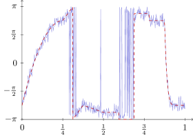
 (a) $f_{\text{o}}$ and $f_{\text{n}}$.

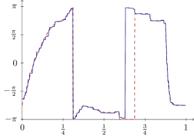
 (b) $\text{TV}_{1}$, $e(f_{\text{o}},f_{\text{r}})\approx 6.06\times 10^{-3}$​.

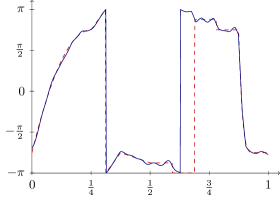
 (c) $\text{TV}_{2}$, $e(f_{\text{o}},f_{\text{r}})\approx 4.34\times 10^{-3}$​.

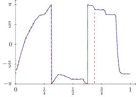
 (d) $\text{TV}_{1}$&$\text{TV}_{2}$, , $e(f_{\text{o}},f_{\text{r}})\approx 3.53\times 10^{-3}$​.

Figure 3: Denoising of an one-dimensional signal by minimizing (43) with CPPA. 3 (a) Original signal $f_{\text{o}}$ (dashed red) and disturbed signal by wrapped Gaussian noise $f_{\text{n}}$ (solid black). 3 (b)—3 (d) Reconstructed signals $f_{\text{r}}$ using 3 (b) only the $\text{TV}_{1}$ regularizer ($\alpha=\frac{3}{4}$), 3 (c) only the $\text{TV}_{2}$ regularizer ($\beta=\frac{3}{2}$), and 3 (d) both of them ($\alpha=\frac{1}{2}$, $\beta=1$). While 3 (b) suffers from the staircasing effect, 3 (c) shows weak results at constant areas. The combination of both regularizers in 3 (d) yields the best image.

The first example of an artificial one-dimensional signal demonstrates the effect of different models containing absolute cyclic first order differences, second order differences or both combined. The function $f:[0,1]\to[-\pi,\pi)$ given by

$$f(x):=\begin{cases}-24\pi x^{2}+\frac{3}{4}\pi&\mbox{ for $0\leq x\leq\frac{1}{4}$,}\\ 4\pi x-\frac{\pi}{4}&\mbox{ for $\frac{1}{4}<x\leq\frac{3}{8}$,}\\ \bigl{(}-\pi x-\frac{3}{8}\bigr{)}_{2\pi}&\mbox{ for $\frac{3}{8}<x\leq\frac{1}{2}$,}\\ \bigl{(}-\frac{j+7}{8}\pi\bigr{)}_{2\pi}&\mbox{ for $\frac{3j+16}{32}<x\leq\frac{3j+19}{32}$, $j=0,1,2,3$,}\\ \frac{3}{2}\pi\exp\bigl{(}-\frac{35}{7}-\frac{1}{1-x}\bigr{)}-\frac{3}{4}\pi&\mbox{ for $\frac{7}{8}<x\leq 1$,}\end{cases}$$

is sampled equidistantly to obtain the original signal $f_{\text{o}}=\Bigl{(}f\bigl{(}\frac{i-1}{N-1}\bigr{)}\Bigr{)}_{i=1}^{N}$ at $N=500$ samples. This function is distorted by wrapped Gaussian noise $\eta$ of standard deviation $\sigma=\frac{1}{5}$ to get $f_{\text{n}}:=\bigl{(}f_{\text{o}}+(\eta)_{2\pi}\bigr{)}_{2\pi}=(f_{\text{o}}+\eta)_{2\pi}$, see also Remark 2.1. The functions $f_{\text{o}}$ and $f_{\text{n}}$ are depicted in Figure 3 (a). Note the following effects due to the cyclic data representation on $[-\pi,\pi)$: The linear increase on $\bigl{[}\frac{1}{4},\frac{3}{8}\bigr{]}$ of $f$ is continuous and the change from $\pi$ to $-\pi$ at $\frac{5}{16}$ is just due to the chosen representation system. Similarly the two constant parts with the values $-\pi$ and $\frac{7}{8}\pi$ differ only by a jump size of $-\frac{\pi}{8}$. For the noise around these two areas, we have the same situation.

We apply Algorithm 1 with different model parameters $\alpha$ and $\beta$ to $f_{\text{n}}$ which yields the restored signals $f_{\text{r}}$. The restoration error is measured by the ‘cyclic’ mean squared error (cMSE) with respect to the arc length distance

$$e(f_{\text{o}},f_{\text{r}}):=\frac{1}{N}\sum_{i=1}^{M}d(f_{\text{o},i},f_{\text{r},i})^{2}.$$

We use $\lambda_{0}=\pi$ and $k=4000$ iterations as stopping criterion. For any choice of parameters $\alpha,\beta$ the computation time is about $6$ seconds.

The result $f_{\text{r}}$ in Figure 3 (b) is obtained using only the $\text{TV}_{1}$ regularization ($\alpha=\frac{3}{4},\beta=0$). The restoration of constant areas is favored by this regularization term, but linear, quadratic and exponential parts suffer from the well-known ‘staircasing’ effect. Utilizing only the $\text{TV}_{2}$ regularization ($\alpha=0,\beta=\frac{2}{3}$) , cf. Figure 3 (c), the restored function becomes worse in flat areas, but shows a better quality in the linear parts. By combining the regularization terms ($\alpha=\frac{1}{2}$, $\beta=1$) as illustrated in Figure 3 (d) both the linear and the constant parts are reconstructed quite well and the cMSE is smaller than for the other choices of parameters. Note that $\alpha$ and $\beta$ were chosen in $\frac{1}{4}\mathbb{N}$ with respect to an optimal cMSE.

5.2 Image denoising of InSAR data

The complex-valued synthetic aperture radar (SAR) data is obtained emitting specific radar signals at equidistant points and measuring the amplitude and phase of their reflections by the earth’s surface. The amplitude provides information about the reflectivity of the surface. The phase encodes both the change of the elevation of the surface’s elements within the measured area and their reflection properties and is therefore rather arbitrary. When taking two SAR images of the target area at the same time but from different angles or locations. The phase difference of these images encodes the elevation, but it is restricted to one wavelength and also includes noise. The result is the so called interferometric synthetic aperture radar (InSAR) data and consists of the ‘wrapped phase’ or the ‘principal phase’, a value in $[-\pi,\pi)$ representing the surface elevation. For more details see, e.g., [9, 33].

After a suitable preregistration the same approach can be applied to two images from the same area taken at different points in time to measure surface displacements, e.g., before and after an earthquake or the movement of glaciers.

The main challenge in order to unwrap the phase is the presence of noise. Ideally, if the surface would be smooth enough and no noise would be present, unwrapping is uniquely determined, i.e., differences between two pixels larger than $\pi$ are regarded as a wrapping result and hence become unwrapped.

There are several algorithms to unwrap, even combining the denoising and the unwrapping, see for example [5, 6]. For denoising, Deledalle et al. [14] use both SAR images and apply a non-local means algorithm jointly to their reflection, the interferometric phase and the coherence.

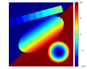
 (a) Original data.

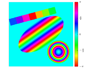
 (b) Wrapped data $f_{\text{o}}$.

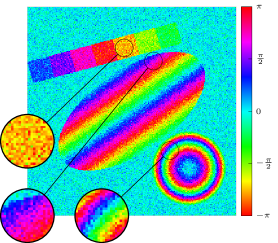
 (c) Noisy data $f_{\text{n}}$.

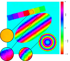
 (d) $\text{TV}_{1}$, $e(f_{\text{o}},f_{\text{r}})=7.09\,\times 10^{-3}$.

 (e) $\text{TV}^{\mathrm{hv}}_{2}$, $e(f_{\text{o}},f_{\text{r}})=6.70\,\times\,10^{-3}$.

 (f) $\text{TV}_{1}$ & $\text{TV}^{\mathrm{hv}}_{2}$, $e(f_{\text{o}},f_{\text{r}})=5.37\,\times\,10^{-3}$.

Figure 4: Denoising of two-dimensional artificial data by minimizing (51) with CPPA. 4 (a) Artificial surface, 4 (b) its wrapped variant, and 4 (c) wrapped image corrupted by wrapped Gaussian noise. 4 (d)–4 (f) Reconstructed images $f_{\text{r}}$ using 4 (d) only the $\operatorname{TV}_{1}$ regularizer ($\alpha=(\frac{3}{8},\frac{1}{4})$), 4 (e) only the $\operatorname{TV}^{\text{hv}}_{2}\,\&\;\operatorname{TV}^{\text{d}}_{2}$ regularizer ($\beta=(\frac{1}{8},\frac{1}{8})$, $\gamma=\frac{1}{8}$), and 4 (f) both of them ($\alpha=(\frac{1}{4},\frac{1}{8})$, $\beta=(\frac{1}{8},\frac{1}{8})$, $\gamma=0$).

Application to synthetic data.

In order to get a better understanding in the two-dimensional case, let us first take a look at a synthetic surface given on $[0,1]^{2}$ with the profile shown in Figure 4 (a). This surface consists of two plates of height $\pm 2\pi$ divided at the diagonal, a set of stairs in the upper left corner in direction $\frac{\pi}{3}$, a linear increasing area connecting both plateaus having the shape of an ellipse with major axis at the angle $\frac{\pi}{6}$, and a half ellipsoid forming a dent in the lower right of the image with circular diameter of size $\frac{9}{25}$ and depth $4\pi$. The initial data is given by sampling the described surface at $M=N=256$ sampling points. The usual InSAR measurement would ideally result in data as given in Figure 4 (b), i.e., the data is wrapped with respect to $2\pi$. In the figure the resulting ideal phase is represented using the hue component of the HSV color space. Again, the data is perturbed by wrapped Gaussian noise, standard deviation $\sigma=0.3$, see Figure 4 (c).

For an application of Algorithm 1 to the minimization problem (51), we have to fix five parameters $\alpha_{1},\alpha_{2},\beta_{1},\beta_{2},\gamma$ which were chosen on $\frac{1}{8}\mathbb{N}$ such that they minimize the cMSE. Using only the cyclic first order differences with $\alpha=\frac{1}{8}(3,2)$, see Figure 4 (d), the reconstructed image $f_{\text{r}}$ reproduces the piecewise constant parts of the stairs in the upper left part and the background, but introduces a staircasing in both linear increasing areas inside the ellipse and in the half ellipsoid. This is highlighted in the three magnifications in Figure 4 (d). Applying only cyclic second order differences with $\beta_{1}=\beta_{2}=\gamma=\frac{1}{8}$ manages to reconstruct the linear increasing part and the circular structure of the ellipsoid, but compared to the first case it even increases the cMSE due to the approximation of the stairs and the background, see especially the magnification of the stairs in Figure 4 (e). Combining first and second order cyclic differences by setting $\alpha_{1}=\alpha_{2}=\frac{1}{8}(2,1)$ and $\beta_{1}=\beta_{2}=\frac{1}{8}$, $\gamma=0$, these disadvantages can be reduced, cf. Figure 4 (f). Note especially the three magnified regions and the cMSE.

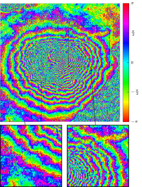
 (a) Complete Vesuvuis data.

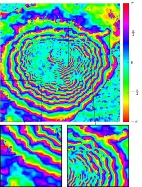
 (b) Denoised Vesuvius data.

Figure 5: 5 (a) Noisy InSAR data set of the Vesuvius taken by the ERS-1 satellite [38]. 5 (b) Denoised image by minimizing (51) with CPPA ($\alpha=\bigl{(}\frac{1}{4},\frac{1}{4}\bigr{)}$, $\beta=\bigl{(}\frac{3}{4},\frac{3}{4}\bigr{)}$ and $\gamma=\frac{3}{4}$).

Application to real-world data.

Next we examine a real-world example. The data from [38] is a set of InSAR data recorded in 1991 by the ERS-1 satellite capturing topographical information from the Mount Vesuvius. The data is available online and a part of it was also used as an example in [50] for TV based denoising of manifold-valued data. In Figure 5 the phase is represented by the hue component of the HSV color space. We apply Algorithm 1 to the image of size $426\times 432$, cf. Figure 5 (a), with  $\alpha_{1}=\alpha_{2}=\frac{1}{4}$ and $\beta_{1}=\beta_{2}=\gamma=\frac{3}{4}$. This reduces the noise while keeping all significant plateaus, ascents and descents, cf. Figure 5 (b). The left zoom illustrates how the plateau in the bottom left of the data is smoothened but kept in its main elevation shown in blue. In the zoom on the right all major parts except the noise are kept. We notice just a little smoothening due to the linearization introduced by $\operatorname{TV}_{2}$. In the bottom left of this detail some of the fringes are eliminated, and a small plateau is build instead, shown in cyan. The computation time for the whole image using $k=600$ iterations as stopping criterion was 86.6 sec and 11.1 sec for each of the details of size $150\times 150$.

6 Conclusions

In this paper we considered functionals having regularizers with second order absolute cyclic differences for $\mathbb{S}^{1}$-valued data. Their definition required a proper notion of higher order differences of cyclic data generalizing the corresponding concept in Euclidian spaces. We derived a CPPA for the minimization of our functionals and gave the explicit expressions for the appearing proximal mappings. We proved convergence of the CPPA under certain conditions. To the best of our knowledge this is the first algorithm dealing with higher order TV-type minimization for $\mathbb{S}^{1}$-valued data. We demonstrated the denoising capabilities of our model on synthetic as well as on real-world data.

Future work includes the application of our higher order methods for cyclic data to other imaging tasks such as segmentation, inpainting or deblurring. For deblurring, the usually underlying linear convolution kernel has to be replaced by a nonlinear construction based on intrinsic (also called Karcher) means. This leads to the task of solving the new associated inverse problem.

Further, we intend to investigate other couplings of first and second order derivatives similar to infimal convolutions or GTV for Euclidean data. Finally, we want to set up higher order TV-like methods for more general manifolds, e.g. higher dimensional spheres. Here, we do not believe that it is possible to derive explicit expressions for the involved proximal mappings – at least not for Riemannian manifolds of nonzero sectional curvature. Instead, we plan to resort to iterative techniques.

Acknowledgement.

We acknowledge the financial support by DFG Grant STE571/11-1.

References

- [1] M. Bačák. Computing medians and means in Hadamard spaces. Preprint, ArXiv, 2013.
- [2] M. Bačák. The proximal point algorithm in metric spaces. Isr. J. Math., 194(2):689–701, 2013.
- [3] D. P. Bertsekas. Incremental gradient, subgradient, and proximal methods for convex optimization: a survey. Technical Report LIDS-P-2848, Laboratory for Information and Decision Systems, MIT, Cambridge, MA, 2010.
- [4] D. P. Bertsekas. Incremental proximal methods for large scale convex optimization. Math. Program., Ser. B, 129(2):163–195, 2011.
- [5] J. Bioucas-Dias, V. Katkovnik, J. Astola, and K. Egiazarian. Absolute phase estimation: adaptive local denoising and global unwrapping. Appl. Optics, 47(29):5358–5369, 2008.
- [6] J. Bioucas-Dias and G. Valadão. Phase unwrapping via graph cuts. IEEE Trans. on Image Process., 16(3):698–709, 2007.
- [7] A. Björck. Numerical Methods for Least Squares Problems. SIAM, Philadelphia, 1996.
- [8] K. Bredies, K. Kunisch, and T. Pock. Total generalized variation. SIAM J. Imaging Sci., 3(3):1–42, 2009.
- [9] R. Bürgmann, P. A. Rosen, and E. J. Fielding. Synthetic aperture radar interferometry to measure earth’s surface topography and its deformation. Annu. Rev. Earth Planet. Sci., 28(1):169–209, 2000.
- [10] A. Chambolle and P.-L. Lions. Image recovery via total variation minimization and related problems. Numer. Math., 76(2):167–188, 1997.
- [11] T. F. Chan, S. Esedoglu, and F. E. Park. Image decomposition combining staircase reduction and texture extraction. J. Vis. Commun. Image R., 18(6):464–486, 2007.
- [12] T. F. Chan, A. Marquina, and P. Mulet. High-order total variation-based image restoration. SIAM J. Sci. Comput., 22(2):503–516, 2000.
- [13] C. Chefd’Hotel, D. Tschumperlé, R. Deriche, and O. Faugeras. Regularizing flows for constrained matrix-valued images. J. Math. Imaging Vis., 20(1-2):147–162, 2004.
- [14] C.-A. Deledalle, L. Denis, and F. Tupin. NL-InSAR: Nonlocal interferogram estimation. IEEE Trans. Geosci. Remote Sensing, 49(4):1441–1452, 2011.
- [15] S. Didas, G. Steidl, and S. Setzer. Combined data and gradient fitting in conjunction with regularization. Adv. Comput. Math., 30(1):79–99, 2009.
- [16] S. Didas, J. Weickert, and B. Burgeth. Properties of higher order nonlinear diffusion filtering. J. Math. Imaging Vis., 35:208–226, 2009.
- [17] O. P. Ferreira and P. R. Oliveira. Proximal point algorithm on Riemannian manifolds. Optimization, 51(2):257–270, 2002.
- [18] N. I. Fisher. Statistical Analysis of Circular Data. Cambridge University Press, 1995.
- [19] P. Fletcher. Geodesic regression and the theory of least squares on Riemannian manifolds. Int. J. Comput. Vision, 105(2):171–185, 2013.
- [20] P. Fletcher and S. Joshi. Riemannian geometry for the statistical analysis of diffusion tensor data. Signal Process., 87(2):250–262, 2007.
- [21] M. Giaquinta, G. Modica, and J. Souček. Variational problems for maps of bounded variation with values in . Calc. Var., 1(1):87–121, 1993.
- [22] M. Giaquinta and D. Mucci. The BV-energy of maps into a manifold: relaxation and density results. Ann. Sc. Norm. Super. Pisa Cl. Sci., 5(4):483–548, 2006.
- [23] M. Giaquinta and D. Mucci. Maps of bounded variation with values into a manifold: total variation and relaxed energy. Pure Appl. Math. Q., 3(2):513–538, 2007.
- [24] P. Grohs, H. Hardering, and O. Sander. Optimal a priori discretization error bounds for geodesic finite elements. Technical Report 2013-16, Seminar for Applied Mathematics, ETH Zürich, Switzerland, 2013.
- [25] P. Grohs and J. Wallner. Interpolatory wavelets for manifold-valued data. Appl. Comput. Harmon. Anal., 27(3):325–333, 2009.
- [26] S. Harizanov, P. Oswald, and T. Shingel. Normal multi-scale transforms for curves. Found. Comput. Math., 11(6):617–656, 2011.
- [27] W. Hinterberger and O. Scherzer. Variational methods on the space of functions of bounded Hessian for convexification and denoising. Computing, 76(1):109–133, 2006.
- [28] S. R. Jammalamadaka and A. SenGupta. Topics in Circular Statistics. World Scientific Publishing Company, 2001.
- [29] S. Lefkimmiatis, A. Bourquard, and M. Unser. Hessian-based norm regularization for image restoration with biomedical applications. IEEE Trans. on Image Process., 21(3):983–995, 2012.
- [30] J. Lellmann, E. Strekalovskiy, S. Koetter, and D. Cremers. Total variation regularization for functions with values in a manifold. In IEEE ICCV 2013, pages 2944–2951, 2013.
- [31] M. Lysaker, A. Lundervold, and X.-C. Tai. Noise removal using fourth-order partial differential equations with applications to medical magnetic resonance images in space and time. IEEE Trans. on Image Process., 12(12):1579–1590, 2003.
- [32] M. Lysaker and X.-C. Tai. Iterative image restoration combining total variation minimization and a second-order functional. Int. J. Comput. Vis., 66(1):5–18, 2006.
- [33] D. Massonnet and K. L. Feigl. Radar interferometry and its application to changes in the Earth’s surface. Rev. Geophys., 36(4):441–500, 1998.
- [34] J. J. Moreau. Fonctions convexes duales et points proximaux dans un espace hilbertien. C. R. Acad. Sci. Paris Ser. A Math., 255:2897–2899, 1962.
- [35] N. Parikh and S. Boyd. Proximity algorithms. Foundations and Trends in Optimization, 1(3):123–231, 2013.
- [36] X. Pennec. Intrinsic statistics on Riemannian manifolds: Basic tools for geometric measurements. J. Math. Imaging Vis., 25(1):127–154, 2006.
- [37] I. U. Rahman, I. Drori, V. C. Stodden, and D. L. Donoho. Multiscale representations for manifold-valued data. Multiscale Model. Simul., 4(4):1201–1232, 2005.
- [38] F. Rocca, C. Prati, and A. M. Guarnieri. Possibilities and limits of SAR interferometry. ESA SP, pages 15–26, 1997.
- [39] R. T. Rockafellar. Monotone operators and the proximal point algorithm. SIAM J. Control Optim., 14(5):877–898, 1976.
- [40] L. I. Rudin, S. Osher, and E. Fatemi. Nonlinear total variation based noise removal algorithms. Physica D., 60(1):259–268, 1992.
- [41] O. Scherzer. Denoising with higher order derivatives of bounded variation and an application to parameter estimation. Computing, 60:1–27, 1998.
- [42] S. Setzer and G. Steidl. Variational methods with higher order derivatives in image processing. In Approximation XII: San Antonio 2007, pages 360–385, 2008.
- [43] S. Setzer, G. Steidl, and T. Teuber. Infimal convolution regularizations with discrete l1-type functionals. Commun. Math. Sci., 9(3):797–872, 2011.
- [44] E. Strekalovskiy and D. Cremers. Total variation for cyclic structures: Convex relaxation and efficient minimization. In IEEE CVPR 2011, pages 1905–1911. IEEE, 2011.
- [45] E. Strekalovskiy and D. Cremers. Total cyclic variation and generalizations. J. Math. Imaging Vis., 47(3):258–277, 2013.
- [46] T. Valkonen, K. Bredies, and F. Knoll. Total generalized variation in diffusion tensor imaging. SIAM J. Imag. Sci., 6(1):487–525, 2013.
- [47] J. Wallner and N. Dyn. Convergence and analysis of subdivision schemes on manifolds by proximity. Comput. Aided Geom. D., 22:593–622, 2005.
- [48] A. Weinmann. Nonlinear subdivision schemes on irregular meshes. Constr. Approx., 31(3):395–415, 2010.
- [49] A. Weinmann. Interpolatory multiscale representation for functions between manifolds. SIAM J. Math. Anal., 44(1):162–191, 2012.
- [50] A. Weinmann, L. Demaret, and M. Storath. Total variation regularization for manifold-valued data. Preprint, ArXiv, 2013.