Asymptotic Reissner-Nordström black holes

Abstract

We consider two types of Born-Infeld like nonlinear electromagnetic fields and obtain their interesting black hole solutions. The asymptotic behavior of these solutions is the same as that of Reissner-Nordström black hole. We investigate the geometric properties of the solutions and find that depending on the value of the nonlinearity parameter, the singularity covered with various horizons.

1 Introduction

Standard Maxwell theory is confronted with the infinite self-energy of charged point-like particles. The renormalization procedure in quantum electrodynamics theory has been applied to obtain a finite value, as deduced from the difference between two infinite forms [1]. The Lagrangian of linear Maxwell field, $L_{Max}=-\mathcal{F}=-F_{\mu\nu}F^{\mu\nu}$, has been considered in various theories of gravity [2]. It is well-known that the Reissner–Nordström (RN) metric is the spherically symmetric solution of Einstein-Maxwell gravity, which corresponds to the charged static black hole of mass $M$ and charge $Q$ [3]. Within gravitational field theories, generalization of RN black holes to nonlinear electromagnetic fields plays a crucial role since most of physical systems are intrinsically nonlinear in the nature.

Among nonlinear electromagnetic fields the well-known Born-Infeld (BI) theory is quite special as low energy limiting cases of certain models of string theory [4]. This classical theory has been designed to regulate the self-energy of a point-like charge [5]. Although coupling of the BI theory with Einstein gravity has been studied in $1935$ [6], in recent years, black hole solutions of BI theory are of interest [7].

Other kinds of nonlinear electrodynamics, with various motivations, in the context of gravitational field have been investigated [8, 9, 10]. In this paper, we consider $(3+1)$-dimensional action of Einstein gravity with two kinds of BI-like nonlinear electromagnetic fields. Generalization of Maxwell field to nonlinear BI model provides powerful tools for investigation of interesting black hole solutions. In addition, it was found that all order loop corrections to gravity may be regarded as a BI-like Lagrangian [11]. Considering the BI Lagrangian

$$L_{BI}=4\beta^{2}\left(1-\sqrt{1+\frac{\mathcal{F}}{2\beta^{2}}}\right),$$ (1)

one can expand it for large values of nonlinearity parameter ($\beta\longrightarrow\infty$) to obtain

$$\left.L_{BI}\right|_{{Large\;}\beta}=-\mathcal{F}+\frac{1}{\beta^{2}}O(\mathcal{F}^{2}),$$ (2)

which confirms that $L_{BI}$ reduces to the linear Maxwell Lagrangian for $\beta\longrightarrow\infty$.

Moreover, from cosmological point of view, it was shown that the early universe inflation may be explained with the nonlinear electrodynamics [12]. Also, one can connect the nonlinear electrodynamics with the large scale correlated magnetic fields observed nowadays [13].

Motivated by all the above, we seek four dimensional solutions to Einstein gravity with the BI-like Lagrangian. We consider a recently proposed BI-like model [14], namely Exponential form of nonlinear electromagnetic field (ENEF) and Logarithmic form of nonlinear electromagnetic field (LNEF), whose Lagrangians are

$$L(\mathcal{F})=\left\{\begin{array}[]{ll}\beta^{2}\left(\exp(-\frac{\mathcal{F}}{\beta^{2}})-1\right),&\;~{}{ENEF}\\ -8\beta^{2}\ln\left(1+\frac{\mathcal{F}}{8\beta^{2}}\right),&\;~{}{LNEF}\end{array}\right..$$ (3)

in which, for large values of $\beta$, $\mathcal{F}^{2}$ correction to Maxwell Lagrangian is included. In other words, the two forms of the mentioned Lagrangians have the same expansion as presented in Eq. (2).

The plan of the paper is as follows. We give a brief review of the simplest coupling of the nonlinear gauge field system (3) to Einstein gravity. Then, we obtain the solutions of the four dimensional spherical symmetric spacetime in the presence of two classes of nonlinear electromagnetic fields, investigate their properties and compare them with BI solution. The paper ends with some conclusions.

2 $(3+1)$-dimensional black holes with nonlinear electromagnetic field

Let us begin with the $(3+1)$-dimensional nonlinear electromagnetic field in general relativity, with the action

$$I_{G}=-\frac{1}{16\pi}\int_{\mathcal{M}}d^{4}x\sqrt{-g}\left[R-2\Lambda+L(\mathcal{F})\right]-\frac{1}{8\pi}\int_{\partial\mathcal{M}}d^{3}x\sqrt{-\gamma}K,$$ (4)

where ${R}$ is the Ricci scalar, $\Lambda$ refers to the negative cosmological constant and $L(\mathcal{F})$ is defined in Eq. (3). In addition, the second integral in Eq. (4) is the boundary term that does not affect the equations of motion, namely the Gibbons-Hawking boundary term [15]. The factors $K$ and $\gamma$ are, respectively, the traces of the extrinsic curvature and the induced metric of boundary ${\partial\mathcal{M}}$ of the manifold ${\mathcal{M}}$. The Einstein and electromagnetic field equations derived from the above action are

$$R_{\mu\nu}-\frac{1}{2}g_{\mu\nu}\left(R-2\Lambda\right)=\alpha\left(\frac{1}{2}g_{\mu\nu}L(\mathcal{F})-2F_{\mu\lambda}F_{\nu}^{\;\lambda}L_{\mathcal{F}}\right),$$ (5)

$$\partial_{\mu}\left(\sqrt{-g}L_{\mathcal{F}}F^{\mu\nu}\right)=0,$$ (6)

where $L_{\mathcal{F}}=\frac{dL(\mathcal{F})}{d\mathcal{F}}$. Our main aim here is to obtain charged static black hole solutions of the field equations (5) and (6) and investigate their properties. We assume a $(3+1)$-dimensional static spacetime is described by the spherically symmetric line element

$$ds^{2}=-f(r)dt^{2}+\frac{dr^{2}}{f(r)}+r^{2}\left(d\theta^{2}+\sin^{2}\theta d\phi^{2}\right).$$ (7)

The electromagnetic tensor $F_{\mu\nu}$ compatible with the metric (7) can involve only a radial electric field $F_{tr}=-F_{rt}$. Therefore, we should use the gauge potential ansatz $A_{\mu}=h(r)\delta_{\mu}^{t}$ in the nonlinear electromagnetic field equation (6). Considering the mentioned ansatz, one can show that Eq. (6) reduces to

$$\begin{array}[]{rr}r\left[1+\left(\frac{2h^{\prime}(r)}{\beta}\right)^{2}\right]h^{\prime\prime}(r)+2h^{\prime}(r)=0,&\;~{}{ENEF\vspace{0.1cm}}\\ r\left[1+\left(\frac{h^{\prime}(r)}{2\beta}\right)^{2}\right]h^{\prime\prime}(r)+2h^{\prime}(r)\left[1-\left(\frac{h^{\prime}(r)}{2\beta}\right)^{2}\right]=0,&\;~{}{LNEF}\end{array},$$ (8)

with the following solutions

$$h(r)=\left\{\begin{array}[]{ll}-\frac{1}{10}\left(4Q^{2}\beta^{2}L_{W}e^{-L_{W}}\right)^{1/4}\left[5+L_{W}F{\left(\left[1\right],\left[\frac{9}{4}\right],\frac{{Lw}}{4}\right)}\right],&\;~{}{ENEF\vspace{0.1cm}}\\ \frac{2Q}{3r}\left[\frac{1}{\left(1+\Gamma\right)}-2F{\left(\left[\frac{1}{4},\frac{1}{2}\right],\left[\frac{5}{4}\right],1-\Gamma^{2}\right)}\right],&\;~{}{LNEF}\end{array}\right.,$$ (9)

where prime and double primes denote the first and second derivative with respect to $r$, respectively, $\Gamma=\sqrt{1+\frac{Q^{2}}{r^{4}\beta^{2}}}$ and $Q$ is an integration constant which is the electric charge of the black holes. In addition, $L_{W}=LambertW\left(\frac{4Q^{2}}{\beta^{2}r^{4}}\right)$ which satisfies $LambertW(x)\exp\left[LambertW(x)\right]=x$ and $F([a],[b],z)$ is hypergeometric function (for more details, see [16]).

It is notable that the same procedure for the linear Maxwell and nonlinear BI theory leads to

$$h(r)=\left\{\begin{array}[]{ll}-\frac{Q}{r},&\;~{}{Maxwell\vspace{0.1cm}}\\ -\frac{Q}{r}F{\left(\left[\frac{1}{4},\frac{1}{2}\right],\left[\frac{5}{4}\right],1-\Gamma^{2}\right)},&\;~{}{BINEF\vspace{0.1cm}}\end{array}\right.$$ (10)

which are completely different with Eq. (9). In order to find the asymptotic behavior of the solutions, we should expand them for large distances ($r>>1$). The radial function $h(r)$ is expanded as

$$\left.h(r)\right|_{{Large\;}r}=-\frac{Q}{r}+\frac{\chi Q^{3}}{20\beta^{2}r^{5}}+O\left(\frac{1}{r^{9}}\right),$$ (11)

where $\chi=2$, $8$ and $1$ for BINEF, ENEF and LNEF, respectively. So, we find that for large values of $r$, the dominant term of Eq. (11) is the gauge potential of RN black hole. Now, we consider the nonvanishing components of $F_{\mu\nu}$. One can show that

$$F_{tr}=-F_{rt}=\frac{Q}{r^{2}}\times\left\{\begin{array}[]{ll}e^{-\frac{L_{W}}{2}},&\;~{}{ENEF}\\ \frac{2}{\Gamma+1},&\;~{}{LNEF}\end{array}\right.,$$ (12)

and it has been shown for BI theory [7]

$$F_{tr}=-F_{rt}=\frac{Q}{\Gamma r^{2}}.$$

Differentiating from Eq. (11) or expanding $F_{tr}$ for large distances, one can obtain

$$F_{tr}=\frac{Q}{r^{2}}-\frac{\chi Q^{3}}{4\beta^{2}r^{6}}+O\left(\frac{1}{r^{10}}\right),$$ (13)

which contain additional radial electric fields apart from the usual Coulomb one.

It is easy to find that all the mentioned electric fields vanish at large values of $r$, as they should be. Furthermore, one may expect to obtain a finite value for the nonlinear electric fields at $r=0$. It is interesting to mention that, despite ENEF, the electric field of LNEF is finite at the origin. One can find that $F_{tr}^{ENEF}$ has a finite value near the origin, which is the same as the electric fields of BINEF and LNEF, but $F_{tr}^{ENEF}$ diverges at $r=0$, as it occurs for Maxwell field.

Now, we should find a suitable function $f(r)$ to satisfy all components of Eq. (5). Considering Eq. (9), one may show that the $rr$ and $tt$ components of Eq. (5) can be simplified as

$$Eq_{tt}=Eq_{rr}=f^{\prime}(r)+\frac{f(r)+\Lambda r^{2}-1}{r}-r\beta^{2}g(r)=0,$$ (14)

where

$$g(r)=\left\{\begin{array}[]{ll}1-\frac{Q}{\beta r^{2}\sqrt{L_{W}}}\left(1-L_{W}\right),&\;~{}{ENEF\vspace{0.2cm}}\\ 4\left[1-\Gamma-\ln\left(\frac{2}{\Gamma+1}\right)\right],&\;~{}{LNEF}\end{array}\right..$$ (15)

Other nonzero components of Eq. (5) can be written as

$$Eq_{\theta\theta}=Eq_{\phi\phi}=\left(\frac{d}{dr}-\frac{1}{r}\right)Eq_{tt}=0,$$ (16)

and therefore it is sufficient to solve $Eq_{tt}=0$. After some cumbersome calculations, the solutions of Eq. (14) can be written as

$$f(r)=1-\frac{2M}{r}-\frac{\Lambda r^{2}}{3}+\left\{\begin{array}[]{ll}\frac{Q}{3}\left(\frac{4Q^{2}\beta^{6}e^{-L_{W}}}{r^{4}L_{W}^{5}}\right)^{1/8}\left[1+L_{W}+\frac{4}{5}L_{W}^{2}F{\left(\left[1\right],\left[\frac{9}{4}\right],\frac{L_{W}}{4}\right)}\right],&\;~{}{ENEF\vspace{0.2cm}}\\ \frac{8Q^{2}F{\left(\left[\frac{1}{2},\frac{1}{4}\right],\left[\frac{5}{4}\right],1-\Gamma^{2}\right)}}{3r^{2}}-\frac{4\beta^{2}r^{2}\left(\Gamma-\ln\left[\frac{\left(\Gamma^{2}-1\right)}{2e^{-7/3}}\right]\right)}{3}-\frac{4\beta^{2}\int r^{2}\ln\left(\Gamma-1\right)dr}{r},&\;~{}{LNEF}\end{array}\right.,$$ (17)

where $M$ is the integration constant which is the total mass of spacetime (the integral term of Eq. (17) will be solved in the appendix). In order to compare our solutions with the BI and RN black holes, we should present the BI and RN solutions. Considering Eq. (10), it has been shown that the field equation (5) reduces to the Eqs. (14) and (16) with

$$g(r)=\left\{\begin{array}[]{ll}\frac{Q^{2}}{r^{3}},&\;~{}{RN\vspace{0.2cm}}\\ 2\left(1-\Gamma\right),&\;~{}{BINEF\vspace{0.2cm}}\end{array}\right.,$$ (18)

and the following solutions

$$f(r)=1-\frac{2M}{r}-\frac{\Lambda r^{2}}{3}+\left\{\begin{array}[]{ll}\frac{Q^{2}}{r^{2}},&\;~{}{RN\vspace{0.2cm}}\\ \frac{4Q^{2}}{3r^{2}}F{\left(\left[\frac{1}{4},\frac{1}{2}\right],\left[\frac{5}{4}\right],1-\Gamma^{2}\right)},&\;~{}{BINEF\vspace{ 0.2cm}}\end{array}\right..$$ (19)

We should note that although Eq. (17) is different with RN and BI solutions, as previously mentioned, they display the same asymptotic behavior. The metric functions of nonlinear electromagnetic fields are expanded as

$$f(r)=1-\frac{2M}{r}-\frac{\Lambda r^{2}}{3}+\frac{Q^{2}}{r^{2}}-\frac{\chi Q^{4}}{40r^{6}\beta^{2}}+O\left(\frac{1}{r^{10}}\right).$$ (20)

Considering the first correction term in Eq. (20), we should stress that the this equation contains both the usual RN terms as well as an analytic function of $O(\frac{1}{r^{6}})$, in which one can ignore it to obtain RN solution for large values of $r$.

In what follows, we are going to investigate the geometric nature of the obtained solutions. At first, we look for the existence of curvature singularities and their horizons. Given the metric in Eq. (7), we can compute the Ricci and the Kretschmann scalars

$$R = -f^{\prime\prime}(r)-\frac{4f^{\prime}(r)}{r}-\frac{2f(r)}{r^{2}},$$ (21)

$$R_{\mu\nu\rho\sigma}R^{\mu\nu\rho\sigma} = f^{\prime\prime 2}(r)+\left(\frac{2f^{\prime}(r)}{r}\right)^{2}+\left(\frac{2f(r)}{r^{2}}\right)^{2}.$$ (22)

where $f(r)$ is the metric function. Also one can show that other curvature invariants (such as Ricci square) are functions of $f^{\prime\prime}$, $f^{\prime}/r$ and $f/r^{2}$, and therefore it is sufficient to study the Ricci and the Kretschmann scalars for the investigation of the spacetime curvature. After a number of manipulations, we find these scalars diverge in the vicinity of the origin

$$\lim_{r\longrightarrow 0^{+}}R = \infty,$$ (23)

$$\lim_{r\longrightarrow 0^{+}}R_{\mu\nu\rho\sigma}R^{\mu\nu\rho\sigma} = \infty,$$ (24)

which confirms that the spacetime given by Eqs. (7) and (17) has an essential singularity at $r=0$.

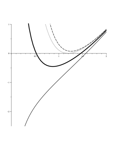
Figure 1: $f(r)$ (ENEF branch) versus $r$ for $\Lambda=-1$, $q=2$, $M=2.5$, and $\beta=0.5<\beta_{c}$ (solid line: black hole with a non-extreme horizon), $\beta_{c}<\beta=1<\beta_{ext}$ (bold line: black hole with two horizons), $\beta=\beta_{ext}=3$ (dotted line: black hole with an extreme horizon) and $\beta=10>\beta_{ext}$ (dashed line: naked singularity)

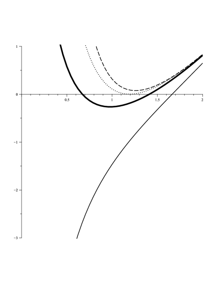
Figure 2: $f(r)$ (LNEF branch) versus $r$ for $\Lambda=-1$, $q=2$, $M=2.5$, and $\beta=0.1<\beta_{c}$ (solid line: black hole with a non-extreme horizon), $\beta_{c}<\beta=0.5<\beta_{ext}$ (bold line: black hole with two horizons), $\beta=\beta_{ext}=1.1$ (dotted line: black hole with an extreme horizon) and $\beta=5>\beta_{ext}$ (dashed line: naked singularity)

In order to investigate the asymptotic behavior of the solution, we should simplify Eqs. (21) and (22) for large distances. Expanding these equations and keep the first order nonlinear correction, we can obtain

$$\lim_{r\longrightarrow\infty}R = 4\Lambda+\frac{\chi Q^{4}}{2\beta^{2}r^{8}}+O\left(\frac{1}{r^{12}}\right),$$ (25)

$$\lim_{r\longrightarrow\infty}R_{\mu\nu\rho\sigma}R^{\mu\nu\rho\sigma} = \frac{8}{3}\Lambda^{2}+\frac{48M^{2}}{r^{6}}-\frac{96MQ^{2}}{r^{7}}+\frac{56Q^{4}}{r^{8}}-\frac{2\chi Q^{4}}{\beta^{2}l^{2}r^{8}}+O\left(\frac{1}{r^{11}}\right),$$ (26)

where the last term is the leading nonlinear correction to the RN black hole solutions. Equations (25) and (26) show that the asymptotic behavior of the obtained solutions is adS for $\Lambda<0$.

Now, we investigate the effects of nonlinear electromagnetic fields and the nonlinearity parameter, $\beta$. Figs. 1 and 2 show that the nonlinearity parameter has effect on the value of the inner and outer horizons in addition to the minimum value of the metric function (when $f(r)$ has a minimum). Furthermore, considering Eq. (19), we find that due to the fact that the metric function of RN black hole is positive near the origin as well as large values of $r$, depending on the value of the metric parameters, one can obtain a black hole with two inner and outer horizons, an extreme black hole with zero temperature and a naked singularity. It is so interesting to mention that for the nonlinear solutions, a new situation may appear. In other words, one can show that near the origin ($r\longrightarrow 0$), the metric function, Eq. (17), may be positive, zero or negative for $\beta>\beta_{c}$, $\beta=\beta_{c}$ or $\beta<\beta_{c}$, respectively (see Figs. 1 and 2 for more details). We should note that considering $\lim_{r\longrightarrow 0^{+}}f(r)=0$, one may obtain $\beta_{c}$ as a function of $\Lambda$, $Q$ and $M$, numerically. The new situation appears for $\beta<\beta_{c}$, in which the black holes have one non-extreme horizon with positive temperature as it happens for (adS) Schwarzschild solutions (uncharged solutions). In addition, Figs. 1 and 2 show that for $\beta>\beta_{c}$, we may obtain an extreme value for the nonlinearity parameter ($\beta_{ext}$) to achieve a black hole with two horizons, an extreme black hole and a naked singularity for $\beta_{c}<\beta<\beta_{ext}$, $\beta=\beta_{ext}$ and $\beta>\beta_{ext}$, respectively.

3 Conclusions

In this paper, we have considered two classes of the BI-like nonlinear electromagnetic fields in the Einsteinian gravity. Expansion of both the mentioned nonlinear Lagrangians, for large values of nonlinearity parameter, is the same as that of BI theory and so we called them BI-like fields.

Regarding four dimensional spherically symmetric spacetime, we have obtained the compatible electromagnetic fields and found that, in contrast with Maxwell field, the mentioned nonlinear electromagnetic fields have finite values in the vicinity of the origin. In addition, we have found that $F_{tr}^{ENEF}$ diverges at $r=0$, but its divergency is much slower than the Maxwell one. In other words, the behavior of the $F_{tr}^{LNEF}$ is very close to BI field, but in the neighborhood of the origin, $F_{tr}^{ENEF}$ has a special behavior between $F_{tr}^{BINEF}$ and $F_{tr}^{RN}$. Expansion of the nonlinear electromagnetic fields for large $r$ showed that the asymptotic behavior of all of them is exactly the same as linear Maxwell field.

Then, we have solved the gravitational field equations and obtained asymptotic AdS solutions with a curvature singularity at $r=0$. We have found that depending on the values of the nonlinearity parameter, $\beta$, the singularity is covered with various horizons. To state the matter differently, we should note that one can obtain two nonlinearity values, $\beta_{c}$ (critical value) and $\beta_{ext}$ (extreme value), in which the singularity covered with a non-extreme horizon for $\beta<\beta_{c}$, two horizons when $\beta_{c}<\beta<\beta_{ext}$, an extreme horizon for $\beta=\beta_{ext}$, and there is a naked singularity otherwise. We have plotted some figures for more clarifications. Finally, we should remark that the ($3+1$)-dimensional nonlinear charged black holes described here have similar asymptotic properties to RN black holes which are well studied.

It would be interesting to carry out a study of the thermodynamic and dynamic properties of the mentioned solutions. Also, it is worthwhile to generalize these four dimensional solutions to the rotating and higher dimensional cases. We leave these problems for future works.

Appendix

In order to complete our discussion, we may solve the following integral

$$\int r^{2}\ln\left(\Gamma-1\right)dr = -\frac{q^{3/2}(\Gamma-1)^{1/4}}{2^{3/4}\beta^{3/2}}\left[\frac{14}{3}F{\left(\left[\frac{1}{4},\frac{1}{4},\frac{11}{4}\right],\left[\frac{5}{4},\frac{5}{4}\right],\frac{1-\Gamma}{2}\right)}-\right.$$

$$\left.\frac{14}{25}(\Gamma-1)F{\left(\left[\frac{5}{4},\frac{5}{4},\frac{11}{4}\right],\left[\frac{9}{4},\frac{9}{4}\right],\frac{1-\Gamma}{2}\right)-}\right.$$

$$\left.\frac{\left[4+3\ln(\Gamma-1)\right]}{9(\Gamma-1)}F{\left(\left[\frac{-3}{4},\frac{7}{4}\right],\left[\frac{1}{4}\right],\frac{1-\Gamma}{2}\right)}+\right.$$

$$\left.\left[-4+\ln(\Gamma-1)\right]F{\left(\left[\frac{1}{4},\frac{7}{4}\right],\left[\frac{5}{4}\right],\frac{1-\Gamma}{2}\right)}\right].$$

References

- [1] L. H. Ryder, Quantum Field Theory Cambridge Univ. Press, (1996).
- [2] A. Chamblin, R. Emparan, C. V. Johnson and R. C. Myers, Phys. Rev. D 60, 064018 (1999); M. H. Dehghani and S. H. Hendi, Phys. Rev. D 73, 084021 (2006); M. H. Dehghani, J. Pakravan and S. H. Hendi, Phys. Rev. D 74, 104014 (2006); M. H. Dehghani, G. H. Bordbar and M. Shamirzaie, Phys. Rev. D 74, 064023 (2006).
- [3] H. Reissner, Ann. Phys. 59, 106 (1916); G. Nordström, Proc. Kon. Ned. Akad. Wet. 20, 1238 (1918).
- [4] N. Seiberg and E. Witten, JHEP 09, 032 (1999); A. A. Tseytlin, [arXiv:hep-th/9908105].
- [5] M. Born and L. Infeld, Proc. R. Soc. London A 143, 410 (1934); M. Born and L. Infeld, Proc. R. Soc. London A 144, 425 (1934).
- [6] B. Hoffmann, Phys. Rev. 47, 877 (1935).
- [7] M. H. Dehghani and H. R. Rastegar-Sedehi, Phys. Rev. D 74, 124018 (2006); D. L. Wiltshire, Phys. Rev. D 38, 2445 (1988); M. Aiello, R. Ferraro and G. Giribet, Phys. Rev. D 70, 104014 (2004); M. H. Dehghani and S. H. Hendi, Int. J. Mod. Phys. D 16, 1829 (2007); M. H. Dehghani, S. H. Hendi, A. Sheykhi and H. R. Rastegar-Sedehi, JCAP, 02, 020 (2007); M. H. Dehghani, N. Alinejadi and S. H. Hendi, Phys. Rev. D 77, 104025 (2008); S. H. Hendi, J. Math. Phys. 49, 082501 (2008).
- [8] M. Hassaine and C. Martinez, Phys. Rev. D 75, 027502 (2007); M. Hassaine and C. Martinez, Class. Quantum Gravit. 25, 195023 (2008); S. H. Hendi and H. R. Rastegar-Sedehi, Gen. Relativ. Gravit. 41, 1355 (2009); S. H. Hendi, Phys. Lett. B 677, 123 (2009); H. Maeda, M. Hassaine and C. Martinez, Phys. Rev. D 79, 044012 (2009); S. H. Hendi and B. Eslam Panah, Phys. Lett. B 684, 77 (2010); S. H. Hendi, Phys. Lett. B 690, 220 (2010); S. H. Hendi, Prog. Theor. Phys. 124, 493 (2010); S. H. Hendi, Eur. Phys. J. C 69, 281 (2010); S. H. Hendi, Phys. Rev. D 82, 064040 (2010).
- [9] H. P. de Oliveira, Class. Quantum Gravit. 11, 1469 (1994).
- [10] B. L. Altshuler, Class. Quantum Gravit. 7, 189 (1990); H. H. Soleng, Phys. Rev. D 52, 6178 (1995).
- [11] E. S. Fradkin and A. A. Tseytlin, Phys. Lett. B 163, 123 (1985); E. Bergshoeff, E. Sezgin, C. N. Pope and P. K. Townsend, Phys. Lett. B 188, 70 (1987); R. R. Metsaev, M. A. Rahmanov and A. A. Tseytlin, Phys. Lett. B 193, 207 (1987); A. A. Tseytlin, Nucl. Phys. B 501, 41 (1997); D. Brecher and M. J. Perry, Nucl. Phys. B 527, 121 (1998).
- [12] R. Garcia-Salcedo and N. Breton, Int. J. Mod. Phys. A 15, 4341 (2000); C. S. Camara, M. R. deGarciaMaia, J. C. Carvalho and J. A. S. Lima, Phys. Rev. D 69, 123504 (2004).
- [13] K. E. Kunze, Phys. Rev. D 77, 023530 (2008); H. J. Mosquera Cuesta and G. Lambiase, Phys. Rev. D 80, 023013 (2009) L. Campanelli , P. Cea, G. L. Fogli and L. Tedesco, Phys. Rev. D 77, 043001 (2008).
- [14] S. H. Hendi, JHEP 03, 065 (2012).
- [15] R. C. Myers, Phys. Rev. D 36, 392 (1987); S. C. Davis, Phys. Rev. D 67, 024030 (2003).
- [16] M. Abramowitz and I. A. Stegun, Handbook of Mathematical Functions, Dover, New York, (1972); R. M. Corless, etal., Adv. Computational Math. 5, 329 (1996).