Synchronization of oscillators in a Kuramoto-type model with generic coupling

Abstract

We study synchronization properties of coupled oscillators on networks that allow description in terms of global mean field coupling. These models generalize the standard Kuramoto-Sakaguchi model, allowing for different contributions of oscillators to the mean field and to different forces from the mean field on oscillators. We present the explicit solutions of self-consistency equations for the amplitude and frequency of the mean field in a parametric form, valid for noise-free and noise-driven oscillators. As an example we consider spatially spreaded oscillators, for which the coupling properties are determined by finite velocity of signal propagation.

Synchronization of large ensembles of oscillators is an ubiquitous phenomenon in physics, engineering, and life sciences. The most simple setup pioneered by Winfree and Kuramoto is that of global coupling, where all the oscillators equally contribute to a mean field which acts equally on all oscillators. In this study we consider a generalized Kuramoto-type model of mean field coupled oscillators with different parameters for all elements. In our setup there is still a unique mean field, but oscillators differently contribute to it with their own phase shifts and coupling factors, and also the mean field acts on each oscillator with different phase shifts and coupling coefficients. Additionally, the noise term is included in the consideration. Such a situation appears, e.g., if the oscillators are spatially arranged and the phase shift and the attenuation due to propagation of their signals cannot be neglected. A regime, where the mean field rotates uniformly, is the most important one. For this case the solution of the self-consistency equation for an arbitrary distribution of frequencies and coupling parameters is found analytically in the parametric form, both for noise-free and noisy oscillators. First, we consider independent distributions for the coupling parameters when self-consistency equations can be greatly simplified. Secondly, we consider an example of a particular geometric organization of oscillators with one receiver that collects signals from oscillators, and with one emitter that sends the driving field on them. By using our approach, synchronization properties can be found for different geometric structures and/or for different parameter distributions.

I Introduction

Kuramoto model of globally coupled phase oscillators lies at the basis of the theory of synchronization of oscillator populations Kuramoto (1984); Acebrón et al. (2005). The model can be formulated as the maximally homogeneous mean field interaction: all oscillators equally contribute to the complex mean field, and this field equally acts on each oscillator (when this action also includes a phase shift, common for all oscillators, one speaks of the Kuramoto-Sakaguchi model Sakaguchi and Kuramoto (1986)). The only complexity in this setup stems from the distribution of the natural frequencies of the oscillators, and from a possibly nontrivial form of the coupling function (which can be e.g. a nonlinear function of the mean field Rosenblum and Pikovsky (2007); Pikovsky and Rosenblum (2009)).

If one considers coupled oscillators on networks, quite a large variety of setups is possible where different oscillators are subject to different inputs, so that mean fields are not involved in the interaction and thus the coupling cannot be described as a global one. In this paper we consider a situation where the oscillators are structured as a specific network that allows one to describe the coupling as a global one. We assume that there is some complex “global field” which involves contributions from individual oscillators, and which acts on all of them. However, contrary to the usual Kuramoto-Sakaguchi setup, we assume the contributions to the global field to be generally different, depending on individual oscillators. Furthermore, the action of this global field on individual oscillators is also different.

Different models having features described above have been studied in the literature. In Hong and Strogatz (2011) the contributions to the global field from all oscillators were the same, but the action on the oscillators was different – some oscillators were attracted to the mean field, and some repelled from it. A generalization of these results on the case of a general distribution of forcing strengths is presented in Iatsenko et al. (2013a). In paper Paissan and Zanette (2008) the authors considered different factors for contributions to the mean field and for the forcing on the oscillators, however no diversity in the phase shifts was studied. In Montbrió and Pazó (2011a) only diversity of these phase shifts was considered.

In this paper we consider a generic Kuramoto-type globally coupled model, where all parameters of the coupling (factors and phases of the contributions of oscillators to the global field, and factors and phases for the forcing of this mean field on the individual oscillators) can be different (cf. Iatsenko et al. (2013b) where such a setup has been recently independently suggested). Furthermore, external noise terms are included in the consideration. We formulate self-consistency conditions for the global field and give an explicit solution of these equations in a parametric form. We illustrate the results with different cases of the coupling parameter distributions. In particular, we consider a situation where the factors and phases of the coupling are determined by a geometrical configuration of the oscillator distribution in space.

II Basic model

We consider a generic system of the Kuramoto-type phase oscillators $\theta_{i}(t)$ having frequencies $\omega_{i}$, with the mean field coupling depicted in Fig. 1. Each oscillator $j$ contributes to the mean field $H(t)$ with its own phase shift $\beta_{j}$ and coupling constant $B_{j}$. The mean field $H(t)$ acts on oscillator $i$ with a specific phase shift $\alpha_{i}$ and a coupling strength $A_{i}$.

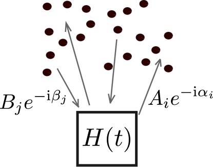
Figure 1: Configuration of the network, coupled via the mean field $H(t)$.

It is convenient to introduce additionally the overall coupling strength $\varepsilon$ (e.g, by normalizing one or both of the introduced quantities $A_{i},B_{j}$; below for definiteness we assume $A_{i},B_{j}>0$ because changing the sign of the coupling can be absorbed to the phase shifts $\beta_{j},\alpha_{i}$) and the overall phase shift $\delta$ (e.g., by normalizing the shifts $\beta_{j},\alpha_{i}$). Additionally we assume that the oscillators are subject to independent Gaussian white noise forces ($\langle\xi_{i}(t)\xi_{j}(t^{\prime})\rangle=2\delta_{ij}\delta(t-t^{\prime})$) with intensity $D$. In this formulation the equations of motions of the oscillators read

$$\dot{\theta}_{i}=\omega_{i}+A_{i}{\varepsilon\over N}\sum_{j=1}^{N}B_{j}\sin(\theta_{j}-\beta_{j}-\theta_{i}+\alpha_{i}-\delta)+\sqrt{D}\xi_{i}(t).$$ (1)

The system (1) can be rewritten in terms of the mean field $H(t)$:

$$\begin{split}\dot{\theta}_{i}&=\omega_{i}+A_{i}\,{\rm Im}\left(H(t)e^{-\text{i}(\theta_{i}-\alpha_{i})}\right)+\sqrt{D}\xi_{i}(t),\\ H(t)&={\varepsilon e^{-\text{i}\delta}\over N}\sum_{j=1}^{N}B_{j}e^{\text{i}(\theta_{j}-\beta_{j})}.\end{split}$$ (2)

It is convenient to reduce the number of parameters by a transformation of phases $\varphi_{i}=\theta_{i}-\alpha_{i}$. Then the equations for $\varphi_{i}$ are:

$$\begin{split}\dot{\varphi}_{i}&=\omega_{i}+A_{i}\,{\rm Im}\left(H(t)e^{-\text{i}\varphi_{i}}\right)+\sqrt{D}\xi_{i}(t),\\ H(t)&={\varepsilon e^{-\text{i}\delta}\over N}\sum_{j=1}^{N}B_{j}e^{\text{i}(\varphi_{j}-\psi_{j})}.\end{split}$$ (3)

where $\psi_{j}=\beta_{j}-\alpha_{j}$.

This model appears to be the most generic one among models of mean-field coupled Kuramoto-type phase oscillators. If all the parameters of the coupling $A_{i},B_{i},\beta_{i},\alpha_{i}$ are constant, then the model reduces to the standard Kuramoto-Sakaguchi one Sakaguchi and Kuramoto (1986). The case with different $A_{i}$, $\alpha_{i}$ and $\omega_{i}$ of specific form has been considered previously in refs. Montbrió and Pazó (2011a, b); *Pazo-Montbrio-11. Also, the case with double delta distribution of $A_{i}$ has been studied in ref. Hong and Strogatz (2011). The case $\alpha_{i}=\beta_{i}=0$ was considered in ref. Paissan and Zanette (2008). In ref. Iatsenko et al. (2013b) the system (1) without noise was examined. Below we formulate the self-consistent equation for this model and present its explicit solution.

It should be noted that the complex mean field $H(t)$ is different from the “classical” Kuramoto order parameter $N^{-1}\sum_{j}e^{\text{i}\varphi_{j}}$ and can be larger than one, depending on the parameters of the system. Because this mean field yields the forcing on the oscillators, it serves as a natural order parameter for this model.

III Self-consistency condition and its solution

Here we formulate, in the spirit of the original Kuramoto approach, a self-consistent equation for the mean field $H(t)$ in the thermodynamic limit, and present its solution. In the thermodynamic limit the quantities $\omega$, $A$, $B$ and $\psi$ have a joint distribution density $g(x)=g(\omega,A,B,\psi)$, where $x$ is a general vector of parameters. While formulating in a general form, we will consider below two specific situations: (i) all the quantities $\omega$, $A$, $B$ and $\psi$ are independent, then $g$ is a product of four corresponding distribution densities; and (ii) situation where the coupling parameters $A$, $B$, and $\psi$ are determined by a geometrical position of an oscillator and thus depend on this position, parametrized by a scalar parameter $x$, while the frequency $\omega$ is distributed independently of $x$.

Introducing the conditional probability density function $\rho(\varphi,t\,|\,x)$, we can rewrite the system (3) as

$$\begin{split}\dot{\varphi}&=\omega+A\,{\rm Im}\left(H(t)e^{-\text{i}\varphi}\right)+\sqrt{D}\xi(t)=\omega+A\,Q\sin(\Theta-\varphi)+\sqrt{D}\xi(t),\\ H(t)&=Qe^{\text{i}\Theta}=\varepsilon e^{-\text{i}\delta}\int g(x)Be^{-\text{i}\psi}\int_{0}^{2\pi}\rho(\varphi,t\,|\,x)e^{\text{i}\varphi}d\varphi\,dx.\end{split}$$ (4)

It is more convenient to write equations for $\Delta\varphi=\varphi-\Theta$, with the corresponding conditional probability density function $\rho(\Delta\varphi,t\,|\,x)=\rho(\varphi-\Theta,t\,|\,x)$:

$$\frac{d}{dt}\Delta\varphi=\omega-\dot{\Theta}-A\,Q\sin(\Delta\varphi)+\sqrt{D}\xi(t),$$ (5)

$$Q=\varepsilon e^{-\text{i}\delta}\int g(x)Be^{-\text{i}\psi}\int_{0}^{2\pi}\rho(\Delta\varphi,t\,|\,x)e^{\text{i}\Delta\varphi}d\Delta\varphi\,dx.$$ (6)

The Fokker-Planck equation for the conditional probability density function $\rho(\Delta\varphi,t\,|\,x)$ follows from (5):

$$\frac{\partial\rho}{\partial t}+\displaystyle\frac{\partial}{\partial\Delta\varphi}\left(\left[\omega-\dot{\Theta}-A\,Q\sin(\Delta\varphi)\right]\rho\right)=D\displaystyle\frac{\partial^{2}\rho}{\partial\Delta\varphi^{2}}.$$ (7)

While one cannot a priori exclude complex regimes in Eq. (7), of particular importance are the simplest synchronous states where the mean field $H(t)$ rotates uniformly (this corresponds to the classical Kuramoto solution). Therefore, we look for such solutions that the phase $\Theta$ of the mean field $H(t)$ rotates with a constant (yet unknown) frequency $\Omega$. Correspondingly, the distribution of phase differences $\Delta\varphi$ is stationary in the rotating with $\Omega$ reference frame (such a solution is often called traveling wave):

$$\dot{\Theta}=\Omega,\ \ \dot{\rho}(\Delta\varphi,t\,|\,x)=0.$$ (8)

Thus, the equation for the stationary density $\rho(\Delta\varphi,t\,|\,x)=\rho(\Delta\varphi\,|\,x)$ reads:

$$\frac{\partial}{\partial\Delta\varphi}\left(\left[\omega-\Omega-A\,Q\sin(\Delta\varphi)\right]\rho\right)=D\displaystyle\frac{\partial^{2}\rho}{\partial\Delta\varphi^{2}}.$$ (9)

Suppose we find solution of (9), which then depends on $Q$ and $\Omega$. Denoting

$$F(\Omega,Q)=\int g(x)Be^{-\text{i}\psi}\int_{0}^{2\pi}\rho(\Delta\varphi,t\,|\,x)e^{\text{i}\Delta\varphi}d\Delta\varphi\,dx\;,$$ (10)

we can then rewrite the self-consistency condition (6) as

$$Q=\varepsilon e^{-\text{i}\delta}F(\Omega,Q)\;.$$ (11)

It is convenient to consider now $Q$, $\Omega$ not as unknowns but as parameters, and to write explicit equations for the coupling strength constants $\varepsilon,\delta$ via these parameters:

$$\varepsilon=\frac{Q}{|F(\Omega,Q)|}\,,\ \ \ \delta=\text{arg}(F(\Omega,Q))\,.$$ (12)

This solution of the self-consistency problem is quite convenient for the numerical implementation, as it reduces to finding of solutions of the stationary Fokker-Planck equation (9) and their integration (10). Below we consider separately how this can be done in the noise-free case and in presence of noise.

IV Noise-free case

In the case of vanishing noise $D=0$ and (9) reduces to

$$\frac{\partial}{\partial\Delta\varphi}\left(\left[\omega-\Omega-A\,Q\sin(\Delta\varphi)\right]\rho\right)=0.$$ (13)

The solution of Eq. (13) depends on the value of the parameter $A$. There are locked phases when $|A|>|\Omega-\omega|/Q$ so $\omega-\Omega-A\,Q\sin(\Delta\varphi)=0$ and rotated phases when $|A|<|\Omega-\omega|/Q$ such that $\rho=C(A,\omega)|\omega-\Omega-A\,Q\sin(\Delta\varphi)|^{-1}$. So the integral over parameter $x$ in (10) splits into two integrals:

$$\begin{split}F(\Omega,Q)&=\int_{|A|>|\Omega-\omega|/Q}g(x)Be^{-\text{i}\psi}\,e^{\text{i}\Delta\varphi(A,\omega)}dx\,+\\ &+\int_{|A|<|\Omega-\omega|/Q}g(x)Be^{-\text{i}\psi}\,C(A,\omega)\int_{0}^{2\pi}\frac{e^{\text{i}\Delta\varphi}\,d\Delta\varphi}{|\omega-\Omega-A\,Q\sin(\Delta\varphi)|}\,dx\,,\end{split}$$ (14)

where in the first integral

$$\sin(\Delta\varphi(A,\omega))=-\frac{\Omega-\omega}{A\,Q}\,,$$

and in the second one

$$C(A,\omega)=\left(\int_{0}^{2\pi}\frac{d\Delta\varphi}{|\omega-\Omega-A\,Q\sin(\Delta\varphi)|}\right)^{-1}\,.$$

Integrations over $\Delta\varphi$ in (14) can be performed explicitely:

$$\begin{split}C(A,\omega)=&\left(\int_{0}^{2\pi}\frac{d\Delta\varphi}{|\omega-\Omega-A\,Q\sin(\Delta\varphi)|}\right)^{-1}=\frac{\sqrt{(\Omega-\omega)^{2}-A^{2}Q^{2}}}{2\pi}\,,\\ &\int_{0}^{2\pi}\frac{e^{\text{i}\Delta\varphi}\,d\Delta\varphi}{|\omega-\Omega-A\,Q\sin(\Delta\varphi)|}=\frac{2\pi\text{i}}{AQ}\left(\frac{\Omega-\omega}{|\Omega-\omega|}-\frac{\Omega-\omega}{\sqrt{(\Omega-\omega)^{2}-A^{2}Q^{2}}}\right)\,.\end{split}$$ (15)

After substitution (15) into (14), we obtain the final general expression for the main function $F(\Omega,Q)$:

$$\begin{split}F(\Omega,Q)&=\int_{|A|>|\Omega-\omega|/Q}g(x)Be^{-\text{i}\psi}\,\sqrt{1-\frac{(\Omega-\omega)^{2}}{A^{2}Q^{2}}\,}\,dx\,-\\ &-\text{i}\int g(x)Be^{-\text{i}\psi}\,\frac{\Omega-\omega}{A\,Q}\,dx\,+\\ &+\text{i}\int_{|A|<|\Omega-\omega|/Q}g(x)Be^{-\text{i}\psi}\,\frac{\Omega-\omega}{|\Omega-\omega|}\sqrt{\frac{(\Omega-\omega)^{2}}{A^{2}Q^{2}}-1\,}\ dx\,.\end{split}$$ (16)

IV.1 Independent parameters

The integrals in (16) simplify in the case of independent distributions of the parameters $\omega$, $A$ and $B$, $\psi$. That means that $g(x)=g_{1}(\omega,A)\,g_{2}(B,\psi)$. In this case it is convenient to consider $\varepsilon$ and $\delta$ as scaling parameters of the distribution $\tilde{g}_{2}(\tilde{B},\tilde{\psi})$, such that

$$\varepsilon e^{-\text{i}\delta}=\int\int\tilde{g}_{2}(\tilde{B},\tilde{\psi})\tilde{B}e^{-\text{i}\tilde{\psi}}d\tilde{B}d\tilde{\psi},$$ (17)

so the parameters $B=\tilde{B}/\varepsilon$ and $\psi=\tilde{\psi}-\delta$ have such a distribution $g_{2}(B,\psi)=\varepsilon\tilde{g}_{2}(\tilde{B},\tilde{\psi})$ that satisfies

$$\int\int g_{2}(B,\psi)Be^{-\text{i}\psi}dBd\psi=1.$$ (18)

From Eq. (18) it follows that Eq. (16) reduces, because the integration over $B$ and $\psi$ yields $1$, to the following expression:

$$\begin{split}F(\Omega,Q)&=\int\int_{|A|>|\Omega-\omega|/Q}g_{1}(\omega,A)\,\sqrt{1-\frac{(\Omega-\omega)^{2}}{A^{2}Q^{2}}\,}\,dAd\omega\,-\\ &-\text{i}\int\int g_{1}(\omega,A)\frac{\Omega-\omega}{A\,Q}\,dAd\omega\,+\\ &+\text{i}\int\int_{|A|<|\Omega-\omega|/Q}g_{1}(\omega,A)\,\frac{\Omega-\omega}{|\Omega-\omega|}\sqrt{\frac{(\Omega-\omega)^{2}}{A^{2}Q^{2}}-1\,}\ dAd\omega\,.\end{split}$$ (19)

Then the parameters $\varepsilon$ and $\delta$ can be found from Eqs. (12) depending on $\Omega$ and $Q$. Noteworthy, all the complexity of distributions of parameters $B$ and $\psi$ is accumulated in values of $\varepsilon$ and $\delta$, while distributions of $\omega,A$ still contribute to the integrals.

Below we give an example of application of our theory. In Fig. 2 we present results of the calculation of the order parameter $Q$ and the frequency of the global field $\Omega$ as function $\varepsilon,\delta$ , for $g_{1}(\omega,A)=g(A)g(\omega)$ and $g(A)=\frac{A}{\theta^{2}}e^{-A/\theta}$, $g(\omega)=\frac{1}{\sqrt{2\pi}}e^{-\omega^{2}/2}$.

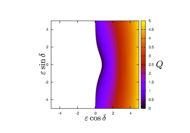
(a) (b)

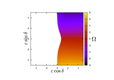
Figure 2: (color online) Dependencies of the amplitude $Q$ of the mean field (a) and of its frequency $\Omega$ on the parameters $\varepsilon$ and $\delta$, for $\theta=1$. White area corresponds to asynchronous state with vanishing mean field.

Furthermore, Eq. (19) simplifies even more when the individual frequencies of the oscillators are identical, i.e. when $g(\omega)=\delta(\omega-\omega_{0})$. Then the integration over $d\omega$ can be performed first:

$$\begin{split}F(\Omega,Q)&=\int_{|A|>|\Omega-\omega_{0}|/Q}g(A)\,\sqrt{1-\frac{(\Omega-\omega_{0})^{2}}{A^{2}Q^{2}}\,}\,dA\,-\\ &-\text{i}\int g(A)\frac{\Omega-\omega_{0}}{A\,Q}\,dA\,+\text{i}\int_{|A|<|\Omega-\omega_{0}|/Q}g(A)\,\frac{\Omega-\omega_{0}}{|\Omega-\omega_{0}|}\sqrt{\frac{(\Omega-\omega_{0})^{2}}{A^{2}Q^{2}}-1\,}\ dA\,.\end{split}$$ (20)

It is convenient to treat the function $F(\Omega,Q)$ in Eq. (20) as a function of a new variable $Y=\frac{\Omega-\omega_{0}}{Q}$, which is a combination of variables $\Omega$ and $Q$. Then Eq. (20) for $F(\Omega,Q)$ transforms to the following equation for $F(Y)$

$$\begin{split}F(Y)&=\int_{|A|>|Y|}g(A)\,\sqrt{1-\frac{Y^{2}}{A^{2}}\,}\,dA\,-\\ &-\text{i}\int g(A)\frac{Y}{A}\,dA\,+\text{i}\int_{|A|<|Y|}g(A)\,\frac{Y}{|Y|}\sqrt{\frac{Y^{2}}{A^{2}}-1\,}\ dA\,,\end{split}$$ (21)

where we took into account that $Q\geq 0$.

Despite the fact that Eqs (12) are still valid for finding $\varepsilon$ and $\delta$, it is more convenient to use $Y$ and $\varepsilon$ as a parameters in Eq. (11) instead of $Q$ and $\Omega$. Then the final expressions for finding $Q$, $\Omega$ and $\delta$ take the following form:

$$Q=\varepsilon\,|F(Y)|\,,\ \ \ \Omega=\omega_{0}+\varepsilon Y\,|F(Y)|\,,\ \ \ \delta=\text{arg}(F(Y))\,.$$ (22)

The results of the calculation of $Q(\varepsilon,\delta)$ and $\Omega(\varepsilon,\delta)$ for the identical natural frequencies are shown in Fig. 3, where we chose $g_{1}(\omega,A)=\frac{A}{\theta^{2}}e^{-A/\theta}\delta(\omega-\omega_{0})$.

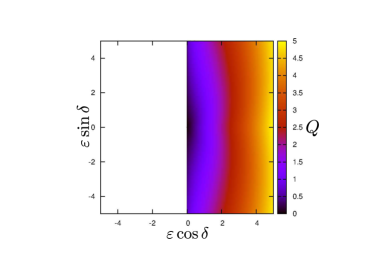
(a) (b)

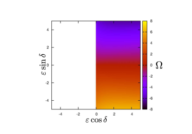
Figure 3: (Color online) Dependencies of the amplitude $Q$ of the mean field (a) and of its frequency $\Omega$ on the parameters $\varepsilon$ and $\delta$, for $\theta=1$ and $\omega_{0}=0$. White area corresponds to asynchronous state with vanishing mean field.

Summarizing this section, we have presented general expressions for the order parameter, frequency of the mean field and the coupling parameters in a parametric form. These expressions are exemplified for specific distributions of the strengths and phase shifts in the couplings in Figs. 2, 3. In the case of a distribution of natural frequencies (Fig. 2) there is a threshold in the coupling for the onset of collective dynamics. For the oscillators with equal frequencies (Fig. 3) there is no threshold.

V Self-consistent solution in the presence of noise

Here we have to find the stationary solution of the Fokker-Planck equation (9). It can be solved in the Fourier modes representation:

$$\rho(\Delta\varphi\,|\,x)=\frac{1}{2\pi}\sum_{n}C_{n}(x)e^{\text{i}n\Delta\varphi}\;,\qquad C_{n}(x)=\int_{0}^{2\pi}\rho e^{-\text{i}n\Delta\varphi}d\Delta\varphi\;,\qquad C_{0}(x)=1\;.$$ (23)

Substituting (23) in Eq. (9), we obtain

$$\begin{split}&\int_{0}^{2\pi}d\Delta\varphi\left[-\frac{\partial}{\partial\Delta\varphi}([\omega-\Omega-AQ\sin(\Delta\varphi)]\rho)+D\frac{\partial^{2}\rho}{\partial\Delta\varphi^{2}}\right]e^{-\text{i}k\Delta\varphi}=\\ &=-k^{2}DC_{k}+\text{i}k(\Omega-\omega)C_{k}+\text{i}kAQ\frac{C_{k-1}-C_{k+1}}{2\text{i}}=0.\end{split}$$ (24)

As a consequence, we get a tridiagonal system of algebraic equations

$$[2kD-\text{i}2(\Omega-\omega)]C_{k}+AQ(C_{k+1}-C_{k-1})=0.$$ (25)

The infinite system (25) can be solved by cutting it at some large $N$, as follows (see ref. Risken (1989)):

$$C_{k}=\alpha_{k}C_{k-1},\quad a_{k}=2kD-\text{i}2(\Omega-\omega)\;,\quad\alpha_{N}=\frac{AQ}{a_{N}}\;,\quad\alpha_{k}=\frac{AQ}{a_{k}+AQ\alpha_{k+1}}.$$ (26)

As a result, $C_{1}$ can be found recursively as a continued fraction:

$$C_{1}=\alpha_{1}=\frac{AQ}{a_{1}+AQ\alpha_{2}}=\ldots\;.$$ (27)

From Eq. (27) it is obvious that in general $C_{1}$ is a function of $\Omega$, $Q$, $\omega$ and $A$:

$$C_{1}=C_{1}(\Omega,Q,\omega,A).$$ (28)

The integral over $\Delta\varphi$ in (10) can be calculated using the Fourier-representation (23), yielding

$$\int_{0}^{2\pi}\rho(\Delta\varphi\,|\,x)e^{\text{i}\Delta\varphi}d\Delta\varphi=C_{1}^{*}(\Omega,Q,\omega,A).$$ (29)

Thus the expression for $F$ in the case of noisy oscillators reads

$$F(\Omega,Q)=\int g(x)Be^{-\text{i}\psi}C_{1}^{*}(\Omega,Q,\omega,A)dx.$$ (30)

V.1 Independent parameters

From the expression (28) it follows that the integral in (30) simplifies in the same case of independent distribution of the parameters $g(x)=g_{1}(\omega,A)\,g_{2}(B,\psi)$, similar to the noise-free case described in the previous section. Here we use the same notations as before, including condition (18).

The parameters $\varepsilon$ and $\delta$ can be found from Eqs. (12), where $F(\Omega,Q)$ is determined from

$$F(\Omega,Q)=\int g_{1}(\omega,A)C_{1}^{*}(\Omega,Q,\omega,A)dAd\omega.$$ (31)

In this way we obtain $Q(\varepsilon,\delta)$ and $\Omega(\varepsilon,\delta)$ (Fig. 4). For calculations we used the same distribution $g_{1}(\omega,A)$ as in the noise-free case.

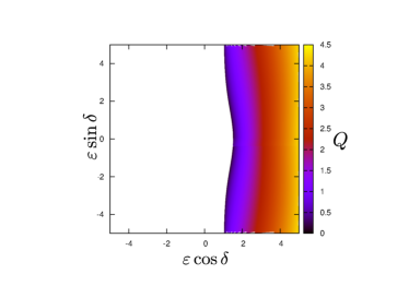
(a) (b)

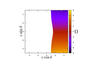
Figure 4: (Color online) The same as Fig. 2, but with noise $D=1$

Contrary to the noise-free case, when oscillator’s individual frequencies are identical (delta-function distribution), no further simplification of $F(\Omega,Q)$ appears possible. In Fig. 5 we report the results for the same parameters as in Fig. 3, but with noise $D=1$.

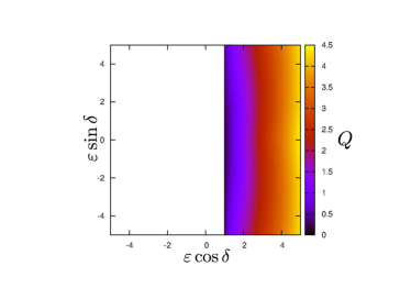
(a) (b)

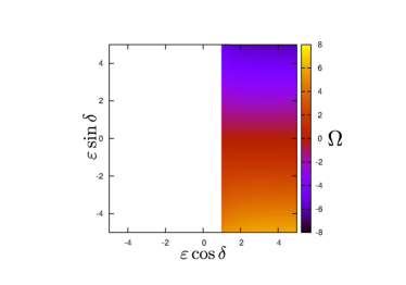
Figure 5: (Color online)The same as Fig. 3, but with noise $D=1$.

In the considered model the main effect caused by noise is the shift of the synchronization threshold to larger values of the coupling strength $\varepsilon$. The noise acts very much similar to the distribution of natural frequencies; if the oscillator’s individual frequencies are identical, noise leads to a non-zero threshold in the coupling.

VI Example of a geometric organization of oscillators

In this section we present a particular example of application of general expressions above to the case where distributions of parameters are determined by configuration of oscillators. We consider spatially spreaded phase oscillators with a common receiver that collects signals from all oscillators, and with an emitter that receives the summarized signal from the receiver and sends the coupling signal to the oscillators; below we assume that these signals propagate with velocity $c$. We assume that the oscillators have the same natural frequencies $\omega_{0}=1$ (cases where the frequencies are distributed (dependent or independent of geometric positions of oscillators) can be straightforwardly treated within the same framework).

We assume that oscillators are distributed uniformly on a circle of radius $r$. Each oscillator is thus labeled by the angle $x_{i}$ (Fig. 6). The receiver, the emitter, and the center of the circle are supposed to lie on one line.

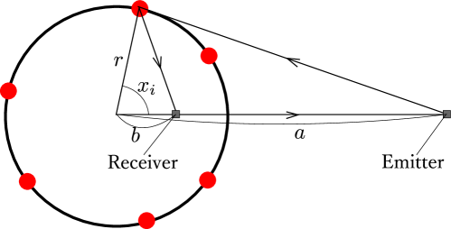
Figure 6: (Color online) The scheme of the system.

Also, we assume that the phase shifts $\beta_{j}$ and $\alpha_{i}$ are proportional to the distances between the oscillator, the receiver and the emitter, so that the system can be described by Eq. (1), where:

$$\beta_{j}={\omega_{0}\over c}\sqrt{r^{2}+b^{2}-2rb\cos x_{j}}\,,\quad\alpha_{i}={\omega_{0}\over c}\sqrt{r^{2}+a^{2}-2ra\cos x_{i}}\,.$$ (32)

Coupling strengths $B_{j}$ and $A_{i}$ are inversely proportional to the square distances between each oscillator, receiver and emitter:

$$B_{j}=\frac{1}{r^{2}+b^{2}-2rb\cos x_{j}},\quad A_{i}=\frac{1}{r^{2}+a^{2}-2ra\cos x_{i}}\;,$$ (33)

where $a$ and $b$ is the distances from the center of the circle to the emitter and the receiver respectively (Fig. 6). The parameters $\varepsilon$ and $\delta$ can be interpreted as a coupling coefficient and a phase shift for the signal transfer from the receiver to the emitter.

The theory developed above yields stable solutions for any given parameters $a$ and $b$. Since all the oscillators have the same natural frequencies, the variable transformation $Y=(\Omega-\omega_{0})/Q$ described in section III should be performed. Thus, it is suitable to use Eqs. (22) in order to find $Q$, $\Omega$ and $\delta$ as a functions of $\varepsilon$ and $Y$.

In the numerical example presented in Fig. 7, we fixed $b=r/2$ and varied $a$, finding the order parameter $Q(a)$ and the frequency of the collective oscillations $\Omega(a)$ for $\varepsilon=1$ and $\delta=0$. One can see a sequence of synchronization regions separated by asynchronous intervals; this is typical for systems with time delay in the coupling – in our case this delay is due to separation of the emitter from the community of oscillators, and the finite speed of signal propagation assumed. The dependencies shown are not smooth, because as parameter $a$ varies, some oscillators enter/leave the synchronization domain.

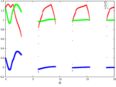
Figure 7: (Color online) The dependance of $Q(a)$, $\Omega(a)$ and $Y(a)$ on the distance from the center of the circle to the emitter $a$, $b=0.5$, $r=1$, $\varepsilon=1$ and $\delta=0$. Periodicity in $a$ corresponds to the zones of attractive and repulsive coupling due to delay-induced phase shift.

VII Conclusion

We have developed a theory of synchronization for phase oscillators on networks with a special structure of coupling through a global mean field. A unified description of the frequency and the amplitude of the mean field in a parametric form is valid both for noise-free and noisy oscillators. In the latter case numerical evaluation of a continued fraction is needed, otherwise the solution reduces to calculation of integrals over parameter distributions. As one of the examples we considered a situation, where contributions to the mean field and its action on oscillators are prescribed by a geometric configuration of the oscillators; phase shifts and the contribution factors result from the propagation of the signals as waves having certain velocity. The general formulation we developed can be used for any such configuration. It appears that the method above may be useful also in more general network setups, where there is no global mean field, but such a field can be introduced as approximation (cf. Skardal and Restrepo (2012); Burioni et al. (2013)).