jahmm: a tool for discretizing multiple ChIP-seq profiles

1 Abstract

Chromatin immunoprecipitation and high throughput sequencing (ChIP-seq) is the de facto standard method to map chromatin features on genomes. The output of ChIP-seq is quantitative within a single genome-wide profile, but there is no natural way to compare experiments, which is why the data is often discretized as present/absent calls. Many tools perform this task efficiently, however they process a single input at a time, which produces discretization conflicts among replicates. Here we present the implementation of a Hidden Markov Model (HMM) using mixture negative multinomial emissions to discretize ChIP-seq profiles. The method gives meaningful discretization for a wide range of features and allows to merge datasets from different origins into a single discretized profile, which resolves discretization conflicts. A quality control step performed after the discretization accepts or rejects the discretization as a whole. The implementation of the model is called jahmm, and it is available as an R package. The source can be downloaded from http://github.com/gui11aume/jahmm.

2 Introduction

The discovery that genes are activated and repressed by transcription factors (proteins that regulate transcription) was the foundation of the modern theory of gene regulation [12]. More recent work on histone post-translational modifications (PTMs) showed that they play a key role in the regulation of transcription. However, the influence of transcription factors and histone PTMs on transcription is still poorly understood, in part because of the discrepancy between their behavior in vivo and in vitro.

Chromatin immunoprecipitation (ChIP) was the first method to address the need to analyze protein-DNA interactions in the context of the nucleus [14]. Earlier methods such as footprinting and electrophoretic mobility shift assays were invaluable in their time, but they could not guarantee that a protein of interest was present on a given sequence of the genome in vivo. The advent of microarrays and later high throughput sequencing gave genome-wide insight into the distribution of transcription factors, but these technologies raised several statistical issues that are still not resolved today. Such methods produce a large amount of data (currently of the order of 100 million reads per run), which calls for efficient and robust analysis methods.

The constant improvement of high throughput sequencing technologies makes the comparison of experiments performed at different dates inconvenient. In addition, it is practically impossible for two laboratories to produce identical ChIP-seq results due to the high number of steps and the complexity of the protocol. For these reasons, the classical approach is to discretize ChIP-seq signals to obtain a call specifying whether the feature of interest is present or absent at every position of the genome. This process is often referred-to as “peak finding” in the biological literature, because transcription factors are believed to bind a single location in a large neighborhood. In practice however, ChIP-seq signals (histone PTMs in particular) often consist of wide domains extending over several Kb.

Many peak finding tools have been developed since the emergence of the ChIP-seq technology, the most popular of which are PeakFinder [6], FindPeaks [3], CisGenome [5], MACS [17], SISSRs [7], BayesPeak [15] and HPeak [13]. BayesPeak and HPeak are based on elaborate statistical models accounting for the overdispersion of ChIP-seq signals and implement a Hidden Markov Model (HMM). However, all these tools can discretize only one ChIP-seq profile at a time, which creates call conflicts when replicates are available. The IDR (Irreproducible Discovery Rate [10]) is an endeavour to solve this issue, but it is restricted to two replicates, meaning that there is no solution for conflict resolution when more than two replicates are available.

Here we present a model addressing this issue. The jahmm (Just Another HMM) discretizer uses an HMM with mixture negative multinomial emissions. This distribution is a good representation of the sequence count at the output of modern sequencers, and it offers an intuitive interpretation as Gamma-Poisson process. The jahmm discretizer not only allows to discretize any ChIP-seq profile, it also allows to combine signals from different sources and/or different technologies into a single discretized profile. Finally, jahmm includes an atomic quality control step that either accepts the discretization or rejects it as a whole.

3 Results

Here we present an accessible overview of jahmm. Mathematical details and complements can be found in the annexes.

3.1 Motivation for the emission model

At the output of a ChIP-seq experiment, we assume that the genome is segmented in windows of identical size and that reads from the sequencer are mapped on the genome and binned in those windows. The number of reads mapping to a genomic window is a discrete variable without upper limit, so the Poisson distribution comes as a natural first guess. However, this choice imposes that the mean number of reads is equal to the variance, which poorly matches experimental observations. It is indeed well known that the distribution of read counts in ChIP-seq experiments is overdispersed [15, 13].

Fig. 1a shows the read count distribution in an experiment performed without immunoprecipitation (the DNA is broken by sonication and sequenced), which describes the baseline distribution of ChIP-seq signals for 300 bp windows. The red histogram shows the distribution of a Poisson variable fitted to the observation. The variance of the observed distribution is more than 3 times larger than the mean and the difference between these distributions is evident for low read counts. For larger windows, the lack of fit of the Poisson distribution becomes more pronounced, as shown in Fig. 1b (in this case the variance is more than 10 times larger than the mean). Discarding non mappable windows reduces the skew but the resulting distribution is not Poisson (data not shown). In summary, the Poisson distribution is not suitable to model ChIP-seq experiments.

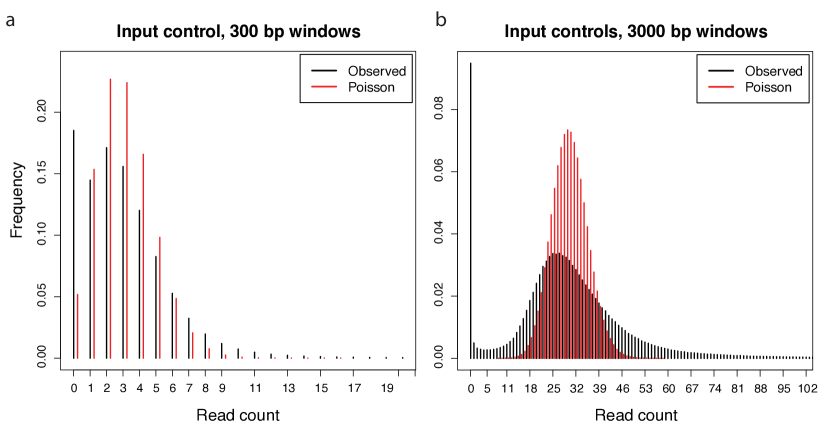
Figure 1: ChIP-seq read count distribution. Left (a): distribution of read counts for a negative control experiment in 300 bp windows (black bars) and the corresponding fitted Poisson distribution (red bars). Notice the lack of fit for the number of windows with no read and for windows with 7 and higher reads. Right (b): same as a for 3000 bp windows.

The negative binomial distribution is more flexibile because it has two parameters, which allows to separate the mean from the variance. More importantly, an intuition of this distribution is given by the two step “Gamma-Poisson mixture”. In the first step, a parameter $\lambda$ is drawn from a Gamma distribution; in the second step, a random observation is drawn from a Poisson distribution with parameter $\lambda$. In other words, the negative binomial distribution can be viewed as a mixture of Poisson distributions with means (i.e. $\lambda$ parameters) distributed as a Gamma random variable.

In the case of ChIP-seq experiments, the mean number of reads mapping to a window is expected to vary due to experimental and computational biases. The G+C content is known to affect the efficiency of the PCR amplification taking place before sequencing. As a consequence, the number of reads is expected to depend on the G+C content of the window. In addition, read mappability is not constant throughout the genome because of polymorphism and repeated sequences, which can decrease the number of mappable reads. These variations are not expected to have an exact Gamma distribution, but since the shape of the Gamma family is flexible, it is a good approximation for many unimodal distributions.

However, the read distribution is clearly bimodal for large windows (Fig. 1b) and is skewed for smaller windows (Fig. 1a). This bimodality is mostly due to the repeated sequences of the genome, since mapping the human genome sequence (hg19) onto itself without any experimental step yields a multimodal distribution (not shown). A mixture of two negative binomial distributions was thus chosen to model the amount of read counts mapping to each genomic window. The mixture model can be estimated efficiently with the EM algorithm [2] and gives a good fit for short windows (Fig. 2a). For 3000 bp windows, the central part of the distribution shows a misfit, but the tails are well captured by the model, which makes it robust to overdispersion. Fitting the right tail is a key property for a discretization model because it reduces the number of false positives compared to the Poisson distribution.

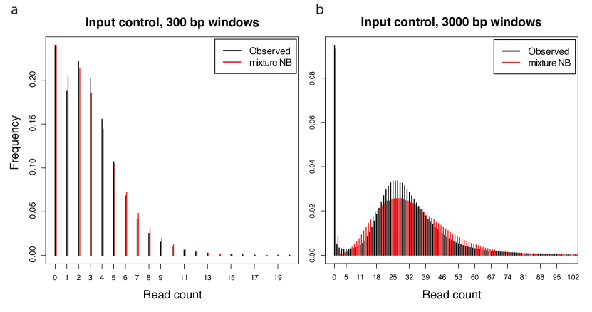
Figure 2: Fit of the mixture negative binomial model. Left (a): same as Fig. 1a, but the red bars represent the corresponding negative binomial mixture distribution fitted by the EM algorithm. Right (b): same as a for 3000 bp windows. The mixture negative binomial model is a good fit for the tail of the distribution.

3.2 Implementation and test

The input of jahmm consists of a set of binned ChIP-seq profiles (assumed to be replicates of each other) plus one negative control ChIP-seq profile binned in the same way. This profile is instrumental to estimate the baseline variations of the read count per window. The output is a single profile of present/absent calls per genomic window. Each ChIP-seq profile represents one dimension of the emissions, modelled by the mixture negative binomial distribution motivated above. We assume that the “shape” parameter of the Gamma distribution underlying the Gamma-Poisson process is a global parameter fixed by the genome and the window size. This means that every genomic window is associated to a reference $\lambda$ parameter, and that the number of reads in each profile have a Poisson distribution with a fixed scaling relative to the reference. These assumptions make the profiles a mixture of negative multinomial variables.

The HMM is assumed to have 3 states, only one of which is interpreted as “present” or “target”; the other 2 are interpreted as “absent”. Hands-on experience with ChIP-seq data shows that many profiles consist of 3 distinct levels (typically “depleted”, “average”, “enriched”) and that low-frequency baseline variations can sometimes capture one state of the HMM, which masks the highest peaks. For these reasons a 3-state model is more robust to process vastly different ChIP-seq data. The full model is fitted using the Baum-Welch algorithm [1], followed by a multi-thread variant of simulated annealing [8] to reduce the chances of being trapped in a local optimum. The present/absent calls are then attributed to each window using the Viterbi algorithm [16], which returns the optimal segmentation under the observations and the fitted model.

Finally, a quality control (QC) for the segmentation is performed using the smoothing distribution of the HMM (the posterior distribution of the states given the emissions). The QC score is the estimated probability of false positives among the “present” calls, which expresses the confidence of the classifier for these calls. In the negative controls we have tested (profiles containing no target), the estimated false positive rate is higher than 0.09 for 300 bp windows. The QC is atomic, in other words the discretization is rejected altogether if the QC score of the sample exceeds this threshold value. Because there are high confidence peaks even in negative controls, it is more meaningful to judge the validity of the discretization, rather than the reliability of each call.

We used jahmm on ENCODE ChIP-seq data [9] for the transcription factor CTCF which is known to bind its targets as single peaks, and for the histone PTM H3K27me3 which is known to be present in the genome in domains. The datasets were produced from the K562 myelogenous leukaemia cell line by different laboratories (five distinct laboratories for CTCF and three for H3K27me3). Fig. 3a and 3b shows that the discretization closely matches the visual expectations in both cases, which is supported by the fact that the QC scores are below the rejection threshold (0.015 and 0.057 respectively).

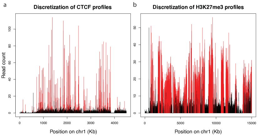
Figure 3: Example discretization by jahmm. Left (a): Discretization of CTCF binding sites. For concision only one of the thirteen profiles used for the discretization is shown. The “present” calls are indicated in red. Right (b): Riscretization of H3K27me3 domains. As for a, only one of the five profiles used for the discretization is shown with the same color code. Notice the different scale of the x axis in both panels.

We also used jahmm to discretize profiles of HDAC6 from a single laboratory. HDAC6 has an overwhelmingly cytosolic distribution [4], it should therefore give a baseline signal with no target. In this case, the discretization proceeded normally, but the QC score was 0.17, exceeding the threshold. This suggests that the discretization of this profile is meaningless. Therefore jahmm can be used to discretize ChIP-seq signals of different types, without prior knowledge of the signal under study, nor of the quality of the experiment.

4 Methods

4.1 ChIP-seq data processing

The raw data .fastq files linked in the supplementary file downloads.lst were downloaded from the ENCODE repository.

Mapping was carried out by gem [11] with options -q ignore -m 2 -T 4 --unique mapping. The versions of gem-indexer and gem-mapper were 1.423 (beta), and 1.376 (beta) respectively. The sequence of the human genome (hg19) in fasta format was downloaded from http://hgdownload.cse.ucsc.edu/goldenPath/hg19/bigZips/chromFaMasked.tar.gz.

In the text, we often refer to the digamma and trigamma functions. The digamma function, noted $\psi(\alpha)$ is the derivative of $\log\Gamma(\alpha)$, and the trigramma function, noted $\psi^{\prime}(\alpha)$ is the derivative of the digamma function.

Appendix A The negative multinomial distribution

A.1 The Gamma-Poisson approach

In what follows, $y$ is a non negative integer (an element of $\mathbb{N}$). Let $Y$ be a discrete random variable distributed according to the Poisson distribution with parameter $\lambda$, denoted $P(\lambda)$. The probability that $Y$ is equal to $y$ is by definition

$$P(Y=y)=e^{-\lambda}\frac{\lambda^{y}}{y!}.$$

Let us now assume that $\lambda$ is itself a random variable, such that the above equality is actually $P(Y=y|\lambda)$. If $\lambda$ has a Gamma distribution with parameters $\alpha$ and $\beta$, the joint distribution of $Y$ and $\lambda$ is written as

$$P(Y=y,\lambda)=e^{-\lambda}\frac{\lambda^{y}}{y!}\frac{1}{\Gamma(\alpha)\beta^{\alpha}}e^{-\lambda/\beta}\lambda^{\alpha-1}.$$

The marginal distribution of $Y$, i.e. $P(Y=y)$, is found by integrating the equality above over $\lambda$.

$$P(Y=y) =\frac{1}{\Gamma(\alpha)\beta^{\alpha}y!}\int_{0}^{+\infty}e^{-\lambda(1+1/\beta)}\lambda^{\alpha+y-1}d\lambda$$

$$=\frac{\Gamma(\alpha+y)}{\Gamma(\alpha)\beta^{\alpha}(1+1/\beta)^{\alpha+y}y!}$$

$$=\frac{\Gamma(\alpha+y)}{\Gamma(\alpha)y!}\left(\frac{1}{1+\beta}\right)^{\alpha}\left(\frac{\beta}{1+\beta}\right)^{y}.$$ (1)

Equation (1) is the expression of the negative binomial distribution, with a somewhat unusual parametrization. We will refer to this distribution as a negative binomial with parameters $(\alpha,1/(1+\beta))$.

A.2 The negative multinomial distribution

As introduced in section A.1, the following equation defines $r$ Poisson variables that are conditionally independent given $\lambda$

$$P(Y_{1}=y_{1},\ldots,Y_{r}=y_{r}|\lambda)=e^{-\gamma_{1}\lambda}\frac{(\gamma_{1}\lambda)^{y_{1}}}{y_{1}!}\times\ldots\times e^{-\gamma_{r}\lambda}\frac{(\gamma_{r}\lambda)^{y_{r}}}{y_{r}!}.$$ (2)

Multiplying by the density of $\lambda$ and integrating as above, the marginal distribution of the vector $(Y_{1},\ldots,Y_{r})$ comes out to

$$P(Y_{1}=y_{1},\ldots,Y_{r}=y_{r}) =\frac{\Gamma(\alpha+y_{1}+\ldots+y_{r})}{\Gamma(\alpha)y_{1}!\ldots y_{r}!}p_{0}^{\alpha}p_{1}^{y_{1}}\ldots p_{r}^{y_{r}},\;\text{where}$$ (3)

$$p_{0} =\frac{1/\beta}{1/\beta+\gamma_{1}+\ldots+\gamma_{r}},\;\text{and}$$

$$p_{i} =\frac{\gamma_{i}}{1/\beta+\gamma_{1}+\ldots+\gamma_{r}},\;\text{for}\;i=1,\ldots,r.$$

This distribution is called the negative multinomial. We will refer to it is as a negative multinomial with parameters $(\alpha,p_{1},\ldots,p_{r})$. We have shown that it can be interpreted as the observations of a Gamma-Poisson process, where a common $\lambda$ value is drawn from a Gamma distribution, and $r$ variables are drawn from independent Poisson distributions with scalings $\gamma_{1},\ldots,\gamma_{r}$ relative to $\lambda$. Note that the variables $Y_{1},\ldots,Y_{r}$ are independent contionally on $\lambda$, but in section A.3 we prove that they are never unconditionally independent.

The parameters of the negative binomial distribution have an alternative interpretation which emphasizes their dependence. Suppose an urn contains black balls and balls of $r$ different colors in respective proportions $p_{0},p_{1},\ldots,p_{r}$. Let us draw balls with replacement from this urn until we draw a black ball for the $k$-th time, and count how many balls of each color we drew. The probability of the $r$-tuple $(y_{1},\ldots,y_{r})$ is easily seen to be

$${k-1+y_{1}+\ldots+y_{r}\choose(k-1),y_{1},\ldots,y_{r}}p_{0}^{k}p_{1}^{y_{1}}\ldots p_{r}^{y_{r}}=\frac{\Gamma(k+y_{1}+\ldots+y_{r})}{\Gamma(k)y_{1}!\ldots y_{r}!}p_{0}^{k}p_{1}^{y_{1}}\ldots p_{r}^{y_{r}}.$$

This is formula (3), where $\alpha$ has been replaced by $k$. The negative multinomial distribution is a generalization of the drawing process described above with non integer values of $k$. The ball and urn interpretation makes it clear that the observed counts $(y_{1},\ldots,y_{r})$ are expected to be twice smaller for a twice larger value of $p_{0}$ or for a twice smaller value of $\alpha$.

A.3 Marginal distributions

Finally, we compute the marginal distributions of $(Y_{1},\ldots,Y_{r})$. Summing (3) is straightforward, but instead we observe that taking the margins of (2) and integrating over $\lambda$ as above yields for $l=1,\ldots,r$

$$P(Y_{l}=y_{l}) =\frac{\Gamma(\alpha+y_{l})}{\Gamma(\alpha)y_{l}!}p_{0}^{*\alpha}p_{l}^{*y_{l}},\;\text{where}$$

$$p_{0}^{*} =\frac{1/\beta}{1/\beta+\gamma_{l}},\;\text{and}$$

$$p_{l}^{*} =\frac{\gamma_{l}}{1/\beta+\gamma_{l}}.$$

Not surprisingly, we obtain a negative binomial distribution. More interestingly though, the parameters of this distribution are linked to the previous parameters by the equality $p_{0}^{*}/p_{l}^{*}=p_{0}/p_{l}$. These constraints are valid for any number of variables in the negative multinomial model, so they come in handy to reparametrize the model every time variables are added or dropped.

As an example of the use of these constraints, we show with $r=2$ that the margins of a negative multinomial distribution are never independent (for the general case, observe that mutual independence entails pairwise independence and that the margins over $r-2$ variables have a negative multinomial distribution). Let us fix $z_{2}=0$. The terms $P(z_{1}=k,z_{2}=0)$ are proportional to $\Gamma(\alpha+k)p_{1}^{k}/k!$ and the terms $P(z_{1}=k)P(z_{2}=0)$ are proportional to $\Gamma(\alpha+k)p_{1}^{*k}/k!$ where $p_{1}^{*}=p_{1}/(p_{1}+p_{0})<p_{1}$ so equality cannot hold for every $k\geq 0$. This shows that the joint distribution is never equal to the product of the marginal distributions.

Note that the proof above assumes $p_{0}>0$, which is a consequence of $\beta<\infty$. So as long as $\lambda$ is distributed according to a proper Gamma distribution, which is a defining feature of the negative multinomial distribution, the variables cannot be independent.

From the marginal distributions we can compute the conditional distribution of $(Y_{1},\ldots,Y_{i})$ given $(Y_{i+1},\ldots,Y_{r})$ (and similary the distribution of any set of variables given the complentary set). Using the same rationale as above, the marginal distribution is found to be negative multinomial with

$$P(Y_{i+1}=y_{i+1},\ldots,Y_{r}=y_{r}) =$$

$$\frac{\Gamma(\alpha+y_{r+1}+\ldots+y_{r})}{\Gamma(\alpha)y_{i+1}!\ldots y_{r}!} p_{0}^{\alpha}p_{i+1}^{y_{i+1}}\ldots p_{r}^{y_{r}}\left(\frac{1}{p_{0}+p_{i+1}+\ldots+p_{r}}\right)^{\alpha+y_{i+1}+\ldots+y_{r}}.$$

The conditional distribution is computed as the ratio of the full distribution and the marginal distribution.

$$P(Y_{1}=y_{1},\ldots,Y_{i}=y_{i}|Y_{i+1}=y_{i+1},\ldots,Y_{r}=y_{r}) =$$

$$\frac{\Gamma(\alpha+y_{1}+\ldots+y_{r})}{\Gamma(\alpha+y_{i+1}+\ldots+y_{r})y_{1}!\ldots y_{i}!} q_{0}^{\alpha+y_{i+1}+\ldots+y_{r}}p_{1}^{y_{1}}\ldots p_{i}^{y_{i}},$$

where $q_{0}=1-(p_{1}+\ldots+p_{i})$. In other words, the distribution of $(Y_{1},\ldots,Y_{i})$ given $(Y_{i+1},\ldots,Y_{r})$ is negative multinomial with parameters $(\alpha+y_{i+1}+\ldots+y_{r},p_{1},\ldots,p_{i})$.

Appendix B Hidden Markov models

We will consider only discrete Hidden Markov models (HMMs) and will simply refer to them as Hidden Markov model, without mention of the term ‘discrete’ for simplicity. HMMs are defined by

1. a set $S$ of $m$ states numbered from 1 to $m$,

2. an initial state probability distribution $\nu$, which gives the probabilities that the system is initially in state $i$,

3. an $m\times m$ transition matrix $Q$ which contains the probabilities $Q(i,j)$ that the system goes from state $i$ to state $j$,

4. $m$ distributions denoted $g_{i}$ $(i=1,\ldots,m)$, which give the emission probabilities in the different states.

B.1 The Forward-Backward algorithm

For a sequence of emissions $y_{0},\ldots,y_{n}$, the likelihood of the state sequence $i_{0},\ldots,i_{n}$ is proportional to

$$\nu(i_{0})g_{i_{0}}(y_{0})\prod_{k=1}^{n}Q(i_{k-1},i_{k})g_{i_{k}}(y_{k}).$$

By summing over all possible combinations of states, we obtain the normalizing constant $L_{n}$ such that

$$L_{n}=\sum_{i_{0}\in S,\ldots,i_{n}\in S}\nu(i_{0})g_{i_{0}}(y_{0})\prod_{k=1}^{n}Q(i_{k-1},i_{k})g_{i_{k}}(y_{k}).$$ (4)

We denote $\phi_{k|n}(i)$ the probability that the system is in state $i$ at time $k$ given the emissions $y_{0},\ldots,y_{n}$. If we call $S_{n}(k,i)$ the set of $n$-tuples $(i_{0},\ldots,i_{n})$ such that $i_{k}=i$, the value of $\phi_{k|n}(i)$ comes as

$$\phi_{k|n}(i)=\frac{1}{L_{n}}\sum_{(i_{0},\ldots,i_{n})\in S_{n}(k,i)}\nu(i_{0})g_{i_{0}}(y_{0})\prod_{l=1}^{n}Q(i_{l-1},i_{l})g_{i_{l}}(y_{l}).$$

We now introduce $\alpha_{k}(i)$ the probability that the system is in state $i$ at time $k$ given the emissions $y_{0},\ldots,y_{k}$, and the $\beta_{k|n}(\cdot)$ the numerical function such that $\phi_{k|n}(i)=\alpha_{k}(i)\beta_{k|n}(i)$.

$$\alpha_{k}(i) =\frac{1}{L_{k}}\sum_{i_{0}=1}^{m}\cdots\sum_{i_{k-1}=1}^{m}\nu(i_{0})g_{i_{0}}(y_{0})\prod_{l=1}^{k-1}Q(i_{l-1},i_{l})g_{i_{l}}(y_{l})Q(i_{k-1},i)g_{i}(y_{k})$$

$$\beta_{k|n}(i) =\frac{L_{k}}{L_{n}}\sum_{i_{k+1}=1}^{m}\cdots\sum_{i_{n}=1}^{m}Q(i,i_{k+1})g_{i_{k+1}}(y_{k+1})\prod_{l=k+2}^{n}Q(i_{l-1},i_{l})g_{i_{l}}(y_{l})$$

To preserve the equality $\phi_{k|n}(i)=\alpha_{k}(i)\beta_{k|n}(i)$ for every $k$, we set by definition $\beta_{n|n}(i)=1$. From the equations above, we draw the following recursive equations:

$$\alpha_{k}(i) =\frac{L_{k-1}}{L_{k}}\sum_{j=1}^{m}\alpha_{k-1}(j)Q(j,i)g_{i}(y_{k})$$ (5)

$$\beta_{k|n}(i) =\frac{L_{k}}{L_{k+1}}\sum_{j=1}^{m}Q(i,j)g_{j}(y_{k+1})\beta_{k+1|n}(j).$$ (6)

Equations (5) and (6) are the basis of the Forward-Backward algorithm to compute $\phi_{k|n}(i)$. The terms $\alpha_{k}(i)$ can be recursively computed from $k=0$ to $k=n$ with equation (5), and the terms $\beta_{k|n}(i)$ can be computed from $k=n-1$ to $k=0$ with equation (6). The terms $\phi_{k|n}(i)$ are then found as the product $\alpha_{k}(i)\beta_{k|n}(i)$.

We now turn to the term $\phi_{k-1,k|n}(i,j)$, which is by definition the probability that the system is in state $i$ at time $k-1$ and in state $j$ at time $k$ given $y_{0},\ldots,y_{n}$. If we call $S_{n}(k,i,j)$ the set of $n$-tuples $(i_{0},\ldots,i_{n})$ such that $i_{k-1}=i$ and $i_{k}=j$, we get

$$\phi_{k-1,k|n}(i,j) =\frac{1}{L_{n}}\sum_{(i_{0},\ldots,i_{n})\in S_{n}(k,i,j)}\nu(i_{0})g_{i_{0}}(y_{0})\prod_{l=1}^{n}Q(i_{l-1},i_{l})g_{i_{l}}(y_{l})$$

$$=\frac{L_{k-1}}{L_{k}}\alpha_{k-1}(i)Q(i,j)g_{j}(y_{k})\beta_{k}(j).$$ (7)

When the $\alpha_{k}(i)$ and the $\beta_{k|n}(i)$ have been computed by the Forward-Backward algorithm, we also have access to the $\phi_{k-1,k|n}(i,j)$ by using formula (7).

B.2 The Baum-Welch algorithm

The Baum-Welch algorithm is the special case of the EM algorithm applied to HMMs. Let us consider the general case of the triplet $(X,Z,\theta)$ where the variable $X$ is observed, $Z$ is not observed, and $\theta$ is the set of parameters of the distribution of $(X,Z)$. The full likelihood $\mathcal{L}_{0}(X,Z,\theta)$ cannot be computed because the value of $Z$ is unknown.

To find the value of $\theta$ that maximizes the full likelihood, we introduce an iterative procedure where the values of the parameter are updated upon each iteration. The current value of $\theta$ is noted $\theta^{(t)}$, and we compute the expected complete log-likelihood $\mathcal{Q}(\theta|\theta^{(t)})$ assuming the current value of $\theta$ (note the difference between the intermediate quantity of the EM $\mathcal{Q}$ and the transition matrix $Q$).

$$\mathcal{Q}(\theta|\theta^{(t)})=E_{Z|X,\theta^{(t)}}\left\{\log\mathcal{L}_{0}(X,Z,\theta^{(t)})\right\}$$

This computation is called the E-step. The notations mean that the expectation is taken over the variable $Z$, assuming that it is conditional on the observed values of $X$ and that the parameters of the distribution are given by $\theta^{(t)}$. The E-step is followed by the M-step, in which $\theta^{(t+1)}$ is set to the value of $\theta$ that maximizes $\mathcal{Q}(\theta|\theta^{(t)})$.

In the case of HMMs, the variable that is not observed is the sequence of states. The set of parameters $\theta^{(t)}$ represents the transition probabilities (the matrix $Q$) and the parameters of the $m$ distributions of the emissions.

The log-likelihood of the state sequence $(i_{0},\ldots,i_{n})$ is

$$\log\nu(i_{0})+\sum_{k=1}^{n}\log Q(i_{l-1},i_{l})+\sum_{k=0}^{n}\log g_{i_{l}}(i_{l},\theta).$$

The addition of $\theta$ to the terms above emphasizes that they depend on the value of the parameters. To compute $\mathcal{Q}(\theta|\theta^{(t)})$, we need to take the expectation of the above over the state sequence conditionally on $y_{0},\ldots,y_{n}$ and assuming that the parameters are given by $\theta^{(t)}$.

$$\mathcal{Q}(\theta|\theta^{(t)}) =E_{\theta^{(t)}}\left\{\log\nu(i_{0})\big{|}y_{0},\ldots,y_{n}\right\}+$$

$$\sum_{k=1}^{n}E_{\theta^{(t)}}\left\{\log Q(i_{l-1},i_{l})\big{|}y_{0},\ldots,y_{n}\right\}+$$ (8)

$$\sum_{k=0}^{n}E_{\theta^{(t)}}\left\{\log g_{i_{l}}(y_{l},\theta)\big{|}y_{0},\ldots,y_{n}\right\}$$

In practice, the first term of (8) will often not depend on $\theta$ so it will not contribute to the evaluation. The third term can be rewritten as

$$\sum_{k=0}^{n}\sum_{i=1}^{m}\phi_{k}(i)\log g_{i_{l}}(y_{l},\theta).$$

This term depends on the emission probabilities, and nothing can be said about it in general terms because they differ between different models. But the second term depends only on the transition probabilities, which are present in every HMM, and it can be solved in general. First we notice that

$$E_{\theta^{(t)}}\left\{\log Q(i_{l-1},i_{l})\big{|}y_{0},\ldots,y_{n}\right\}=$$

$$E_{\theta^{(t)}}\left\{\sum_{i=1}^{m}\sum_{j=1}^{m}1_{\{(i_{l-1},i_{l})=(i,j)\}}\log Q(i,j)\big{|}y_{0},\ldots,y_{n}\right\}=$$

$$\sum_{i=1}^{m}\sum_{j=1}^{m}E_{\theta^{(t)}}\left\{1_{\{(i_{l-1},i_{l})=(i,j)\}}\big{|}y_{0},\ldots,y_{n}\right\}\log Q(i,j)$$

Remember that by definition $E_{\theta^{(t)}}\left\{1_{\{(i_{l-1},i_{l})=(i,j)\}}\big{|}y_{0},\ldots,y_{n}\right\}$ is $\phi_{k-1,k}(i,j)$, so that we can rewrite the second term of (8) as

$$\sum_{k=1}^{n}\sum_{i=1}^{m}\sum_{j=1}^{m}\phi_{k-1,k}(i,j)\log Q(i,j).$$

The values of $\phi_{k-1,k}(i,j)$ are computed during the E-step by the Forward-Backward algorithm. The terms $Q(i,j)$ are part of $\theta$ and are thus updated during the M-step. By using Lagrange multipliers, we can show that the update values are

$$Q(i,j)^{(t+1)}=\frac{\sum_{k=1}^{n}\phi_{k-1,k}(i,j)}{\sum_{k=1}^{n}\sum_{l=1}^{m}\phi_{k-1,k}(i,l)}.$$

To complete the Baum-Welch algorithm, we need to compute the last term of (8), which requires making a model for the emissions.

Appendix C Negative multinomial emissions

The readout of ChIP-seq and similar experiments is a sequence of reads mapped to genomic windows of identical size. The negative multinomial distribution is a good choice to describe the number of reads per window for the following reasons:

1. it is a discrete random variables with values in $\mathbb{N}$.

2. section A shows that it can be interpreted as a Poisson distribution where the parameter $\lambda$ varies as a Gamma variable. With this interpretation, each genomic window has a different expected read number. Conditionally on that number, the read count for a given window is a Poisson variable.

We further assume that $r$ experiments are available. For a given genomic window and a given state $x_{i}$, the probability of observing $(z_{1},\ldots,z_{r})$ reads in the available profiles is

$$\frac{\Gamma(\alpha+z_{1}+\ldots+z_{r})}{\Gamma(\alpha)z_{1}!\ldots z_{r}!}p_{0,i}^{\alpha}\;p_{1,i}^{z_{1}}\ldots p_{r,i}^{z_{r}}$$

The log-likelihood is thus proportional to

$$\log\Gamma(\alpha+z_{1}+\ldots+z_{r}) -\log\Gamma(\alpha)+$$

$$\alpha\log(p_{0,i}) +z_{1}\log(p_{1,i})+\ldots+z_{r}\log(p_{r,i})$$

The third term of (8) is then (up to an additive constant)

$$\ell= -n\log\Gamma(\alpha)+\sum_{k=1}^{n}\log\Gamma(\alpha+z_{k,1}+\ldots+z_{k,r})+$$ (9)

$$\sum_{i=1}^{m}\sum_{k=1}^{n}\phi_{k|n}(i)\Big{(}\alpha\log(p_{0,i})+z_{k,1}\log(p_{1,i})+\ldots+z_{k,r}\log(p_{r,i})\Big{)}.$$ (10)

The maximum is found by differentiation as shown below. We start by differentiating with respect to the parameters $p_{0,i},\ldots,p_{r,i}$, which are bound by the constraint $p_{0,i}+\ldots+p_{r,i}=1$.

$$\frac{\partial\ell}{\partial p_{0,i}}=\frac{\alpha}{p_{0,i}}\sum_{k=1}^{n}\phi_{k|n}(i)=\lambda$$ (11)

$$\frac{\partial\ell}{\partial p_{l,i}}=\frac{1}{p_{l,i}}\sum_{k=1}^{n}\phi_{k|n}(i)z_{k,l}=\lambda,\;l=1,\ldots,r.$$ (12)

The solution of equations (11) and (12) is given by

$$p_{0,i} =\frac{\alpha}{\alpha+\bar{z}_{1,i}+\ldots+\bar{z}_{r,i}}$$ (13)

$$p_{l,i} =\frac{\bar{z}_{l,i}}{\alpha+\bar{z}_{1,i}+\ldots+\bar{z}_{r,i}},\;\text{where}$$ (14)

$$\bar{z}_{l,i} =\frac{\sum_{k=1}^{n}\phi_{k|n}(i)z_{l,i}}{\sum_{k=1}^{n}\phi_{k|n}(i)}\;(l=1,\ldots,r).$$ (15)

Equation (13) is then used to obtain an equation in $\alpha$ by substitution.

$$\frac{\partial\ell}{\partial\alpha} =-n\psi(\alpha)+\sum_{k=1}^{n}\psi(\alpha+z_{k,1}+\dots+z_{k,r})+\sum_{i=1}^{m}\sum_{k=1}^{n}\phi_{k|n}(i)\log(p_{0,i})$$

$$=n(\log(\alpha)-\psi(\alpha))+\sum_{k=1}^{n}\psi(\alpha+z_{k,1}+\dots+z_{k,r})$$

$$-\sum_{i=1}^{m}\log(\alpha+\bar{z}_{1,i}+\ldots+\bar{z}_{r,i})\sum_{k=1}^{n}\phi_{k|n}(i)$$ (16)

The equation $\partial\ell/\partial\alpha\equiv f(\alpha)=0$ is solved by the Newton-Raphson method. For this we need to use the update formula $\alpha^{(t+1)}=\alpha^{(t)}-f(\alpha^{(t)})/f^{\prime}(\alpha^{(t)})$, which depends on $f^{\prime}(\alpha)$ which is computed as show below.

$$f^{\prime}(\alpha) =n\left(1/\alpha-\psi^{\prime}(\alpha)\right)+\sum_{k=1}^{n}\psi^{\prime}(\alpha+y_{k}+z_{k,1}+\ldots+z_{k,r})$$

$$-\sum_{i=1}^{m}\frac{1}{\alpha+\bar{z}_{1,i}+\ldots+\bar{z}_{r,i}}\sum_{k=1}^{n}\phi_{k|n}(i)$$

Appendix D Negative binomial mixture model

In a negative binomial mixture model, every observation is drawn from a finite set of negative binomial distributions. Here we will only consider the case of two distributions. More specifically we will consider that the observations are drawn from a negative binomial with parameters $(\alpha,p)$ with probability $\theta$ and from a negative binomial with parameters $(\alpha,q)$ with probability $1-\theta$. The distribution is thus

$$P(Y=y)=\frac{\Gamma(\alpha+y)}{\Gamma(\alpha)y!}\left(\theta p^{\alpha}(1-p)^{y}+(1-\theta)q^{\alpha}(1-q)^{y}\right).$$ (17)

Mixture distributions are commonly fitted by the EM algorithm. We suppose that an unobserved variable $Z$ takes value 1 with probability $\theta$ and value 0 with probability $1-\theta$. Obivously, $Z$ indicates which of the two distributions the observation is drawn from. The full likelihood is

$$P(y,z)=\frac{\Gamma(a+y)}{\Gamma(\alpha)y!}\left(\theta^{z}p^{\alpha}(1-p)^{y}+(1-\theta)^{1-z}q^{\alpha}(1-q)^{y}\right).$$

This immediately leads to the observation that

$$P(Z=1|Y=y)=\frac{\theta p^{\alpha}(1-p)^{y}}{\theta p^{\alpha}(1-p)^{y}+(1-\theta)q^{\alpha}(1-q)^{y}}.$$ (18)

The E-step of the algorithm is to write the expected log-likelihood of the distribution with respect to the conditional distribution of $Z$. If we write $\theta_{k}=P(Z_{k}=1|Y=y_{k})$ and drop the constant term, this quantity is

$$\ell=-n\log\Gamma(\alpha) +\sum_{k=1}^{n}\log\Gamma(\alpha+y_{k})+\theta_{k}(\log(\theta)+\alpha\log(p)+y_{k}\log(1-p))+$$

$$\;\;(1-\theta_{k})(\log(1-\theta)+\alpha\log(q)+y_{k}\log(1-q)).$$ (19)

The M-step is to maximize (19), which is done by differentiation. Introducing $\bar{y}_{1}=\sum_{k=1}^{n}\theta_{k}y_{k}/\sum_{k=1}^{n}\theta_{k}$ and $\bar{y}_{0}=\sum_{k=1}^{n}(1-\theta_{k})y_{k}/\sum_{k=1}^{n}(1-\theta_{k})$, it is easily verified that at the optimum

$$\theta =\frac{1}{n}\sum_{k=1}^{n}\theta_{k}$$

$$p =\frac{\alpha}{\alpha+\bar{y}_{1}}$$

$$q =\frac{\alpha}{\alpha+\bar{y}_{0}}.$$

By substituting those values in $\partial\ell/\partial\alpha$, we obtain an expression $f(\alpha)$ that depends on $\alpha$ only

$$f(\alpha)=n\left((\log(\alpha)-\psi(\alpha)\right)+\sum_{k=1}^{n}\psi(\alpha+y_{k})+\theta_{k}\log(\alpha+\bar{y}_{1})+(1-\theta_{k})\log(\alpha+\bar{y}_{0})$$

We need to find the solution of $f(\alpha)=0$, which is done by the Newton-Raphson method. For this, we use the update formula $\alpha_{i+1}=\alpha_{i}-f(\alpha_{i})/f^{\prime}(\alpha_{i})$, where

$$f^{\prime}(\alpha)=n\left(1/\alpha-\psi^{\prime}(\alpha)\right)+\sum_{k=1}^{n}\psi^{\prime}(\alpha+y_{k})+\frac{\theta_{k}}{\alpha+\bar{y}_{1}}+\frac{1-\theta_{k}}{\alpha+\bar{y}_{0}}.$$

Summary of the jahmm EM algorithm:

Assuming that the initial parameter values $\alpha_{0},\theta_{0},p_{0},q_{0}$ are available, do the following:

1. For $k=1,\ldots,n$ compute

   $$\theta_{k}=\frac{\theta_{t}p_{t}^{\alpha_{t}}(1-p_{t})^{y_{k}}}{\theta_{t}p_{t}^{\alpha_{t}}(1-p_{t})^{y_{k}}+(1-\theta_{t})q_{t}^{\alpha_{t}}(1-q_{t})^{y_{k}}}.$$

2. Compute

   $$\bar{y}_{1} =\frac{\sum_{k=1}^{n}\theta_{k}y_{k}}{\sum_{k=1}^{n}\theta_{k}},$$

   $$\bar{y}_{0} =\frac{\sum_{k=1}^{n}(1-\theta_{k})y_{k}}{\sum_{k=1}^{n}(1-\theta_{k})}.$$

3. Update $\alpha$ by the Newton-Raphson scheme. Starting with $\tilde{\alpha}_{0}=\alpha_{t}$, update the value of $\tilde{\alpha}$ with the formula $\tilde{\alpha}_{i+1}=\tilde{\alpha}_{i}-f(\tilde{\alpha}_{i})/f^{\prime}(\tilde{\alpha}_{i})$, where

   $$f(\tilde{\alpha}_{i}) =n\left((\log(\tilde{\alpha}_{i})-\psi(\tilde{\alpha}_{i})\right)+$$

   $$\sum_{k=1}^{n}\psi(\tilde{\alpha}_{i}+y_{k})+\theta_{k}\log(\tilde{\alpha}_{i}+\bar{y}_{1})+(1-\theta_{k})\log(\tilde{\alpha}_{i}+\bar{y}_{0}),\;\text{and}$$

   $$f^{\prime}(\tilde{\alpha}_{i}) =n\left(1/\tilde{\alpha}_{i}-\psi^{\prime}(\tilde{\alpha}_{i})\right)+\sum_{k=1}^{n}\psi^{\prime}(\tilde{\alpha}_{i}+y_{k})+\frac{\theta_{k}}{\tilde{\alpha}_{i}+\bar{y}_{1}}+\frac{1-\theta_{k}}{\tilde{\alpha}_{i}+\bar{y}_{0}}.$$

   Stop iterations when $|\tilde{\alpha}_{i+1}-\tilde{\alpha}_{i}|<\varepsilon$ for a chosen $\varepsilon$, and set $\alpha_{t+1}=\tilde{\alpha}_{i+1}$.

4. Update $\theta$, $p$ and $q$ by

   $$\theta_{t+1} =\frac{1}{n}\sum_{k=1}^{n}\theta_{k}$$

   $$p_{t+1} =\frac{\alpha_{t+1}}{\alpha_{t+1}+\bar{y}_{1}}$$

   $$q_{t+1} =\frac{\alpha_{t+1}}{\alpha_{t+1}+\bar{y}_{0}}.$$

5. If the values of $\alpha$, $\theta$, $p$ and $q$ are stable stop the algorithm, otherwise start another cycle.

Appendix E Negative multinomial mixture emissions

The parameters $\alpha$ and $\theta$ can be estimated from the reads counts of the negative control $(y_{1},\ldots,y_{n})$ by the EM algorithm as shown in section D. We now turn to the Baum-Welch algorithm under the assumptions that the observations in each profile are drawn from a negative binomial mixture distribution of which the parameters $\alpha$ and $\theta$ are the same.

Dropping the constants terms (also including $\alpha$ which is now fixed), expression (10) is replaced by

$$\ell=\sum_{i=1}^{m}\sum_{k=1}^{n}\phi_{k|n}(i)\log\Big{(}\theta p_{0,i}^{\alpha}\,p_{1,i}^{z_{k,1}}\ldots p_{r,i}^{z_{k,r}}+(1-\theta)q_{0,i}^{\alpha}\,q_{1,i}^{z_{k,1}}\ldots q_{r,i}^{z_{k,r}}\Big{)}.$$

For simplicity, we introduce the terms $\theta_{k}(i)$ for $k=1,\ldots,n$ and $i=1,\ldots,m$ defined by

$$\theta_{k}(i)=\frac{\theta p_{0,i}^{\alpha}\,p_{1,i}^{z_{k,1}}\ldots p_{r,i}^{z_{k,r}}}{\theta p_{0,i}^{\alpha}\,p_{1,i}^{z_{k,1}}\ldots p_{r,i}^{z_{k,r}}+(1-\theta)q_{0,i}^{\alpha}\,q_{1,i}^{z_{k,1}}\ldots q_{r,i}^{z_{k,r}}},$$ (20)

and the terms $\bar{z}_{l,i}^{*}$ for $l=1,\ldots,r$ and $i=1,\ldots,m$ defined by

$$\bar{z}_{l,i|1}^{*} =\frac{\sum_{k=1}^{n}\phi_{k|n}(i)\theta_{k}(i)z_{l,i}}{\sum_{k=1}^{n}\phi_{k|n}(i)\theta_{k}(i)},$$

$$\bar{z}_{l,i|0}^{*} =\frac{\sum_{k=1}^{n}\phi_{k|n}(i)(1-\theta_{k}(i))z_{l,i}}{\sum_{k=1}^{n}\phi_{k|n}(i)(1-\theta_{k}(i))}.$$

Using a similar strategy as the EM, we can fix the $\theta_{k}(i)$ and treat them as constants. The solution is subject to the constaints $p_{0,i}+\ldots+p_{r,i}=1$, $q_{0,i}+\ldots+q_{r,i}=1$, $p_{0,i}/p_{1,i}=C_{1}$ and $q_{0,i}/q_{1,i}=C_{2}$. Using Lagrange multipliers, we easily find that

$$p_{0,i} =\frac{C_{1}}{C_{1}+1}\cdot\frac{\alpha+\bar{z}_{1,i|1}^{*}}{\alpha+\bar{z}_{1,i|1}^{*}+\ldots+\bar{z}_{r,i|1}^{*}},$$

$$p_{1,i} =\frac{1}{C_{1}+1}\cdot\frac{\alpha+\bar{z}_{1,i|1}^{*}}{\alpha+\bar{z}_{1,i|1}^{*}+\ldots+\bar{z}_{r,i|1}^{*}},$$

$$p_{l,i} =\frac{\bar{z}_{l,i|1}^{*}}{\alpha+\bar{z}_{1,i|1}^{*}+\ldots+\bar{z}_{r,i|1}^{*}},\;(l=2,\ldots,r).$$

and

$$q_{0,i} =\frac{C_{2}}{C_{2}+1}\cdot\frac{\alpha+\bar{z}_{1,i|0}^{*}}{\alpha+\bar{z}_{1,i|0}^{*}+\ldots+\bar{z}_{r,i|0}^{*}},$$

$$q_{1,i} =\frac{1}{C_{2}+1}\cdot\frac{\alpha+\bar{z}_{1,i|0}^{*}}{\alpha+\bar{z}_{1,i|0}^{*}+\ldots+\bar{z}_{r,i|0}^{*}},$$

$$q_{l,i} =\frac{\bar{z}_{l,i|0}^{*}}{\alpha+\bar{z}_{1,i|0}^{*}+\ldots+\bar{z}_{r,i|0}^{*}},\;(l=2,\ldots,r).$$

The new values of $\theta_{k}(i)$ are then recomputed by formula (20). Those EM-like cycles are repeated until convergence.

References

- [1] Leonard E. Baum and Ted Petrie. Statistical inference for probabilistic functions of finite state markov chains. The Annals of Mathematical Statistics, 37(6):1554–1563, 12 1966.
- [2] A. P. Dempster, N. M. Laird, and D. B. Rubin. Maximum likelihood from incomplete data via the em algorithm. JOURNAL OF THE ROYAL STATISTICAL SOCIETY, SERIES B, 39(1):1–38, 1977.
- [3] Anthony P Fejes, Gordon Robertson, Mikhail Bilenky, Richard Varhol, Matthew Bainbridge, and Steven J M Jones. FindPeaks 3.1: a tool for identifying areas of enrichment from massively parallel short-read sequencing technology. Bioinformatics, 24(15):1729–30, August 2008.
- [4] Charlotte Hubbert, Amaris Guardiola, Rong Shao, Yoshiharu Kawaguchi, Akihiro Ito, Andrew Nixon, Minoru Yoshida, Xiao-Fan Wang, and Tso-Pang Yao. HDAC6 is a microtubule-associated deacetylase. Nature, 417(6887):455–8, May 2002.
- [5] Hongkai Ji, Hui Jiang, Wenxiu Ma, David S Johnson, Richard M Myers, and Wing H Wong. An integrated software system for analyzing ChIP-chip and ChIP-seq data. Nat. Biotechnol., 26(11):1293–300, November 2008.
- [6] David S Johnson, Ali Mortazavi, Richard M Myers, and Barbara Wold. Genome-wide mapping of in vivo protein-DNA interactions. Science, 316(5830):1497–502, June 2007.
- [7] Raja Jothi, Suresh Cuddapah, Artem Barski, Kairong Cui, and Keji Zhao. Genome-wide identification of in vivo protein-DNA binding sites from ChIP-Seq data. Nucleic Acids Res., 36(16):5221–31, September 2008.
- [8] S Kirkpatrick, C D Gelatt, and M P Vecchi. Optimization by simulated annealing. Science, 220(4598):671–80, May 1983.
- [9] Stephen G Landt, Georgi K Marinov, Anshul Kundaje, Pouya Kheradpour, Florencia Pauli, Serafim Batzoglou, Bradley E Bernstein, Peter Bickel, James B Brown, Philip Cayting, Yiwen Chen, Gilberto DeSalvo, Charles Epstein, Katherine I Fisher-Aylor, Ghia Euskirchen, Mark Gerstein, Jason Gertz, Alexander J Hartemink, Michael M Hoffman, Vishwanath R Iyer, Youngsook L Jung, Subhradip Karmakar, Manolis Kellis, Peter V Kharchenko, Qunhua Li, Tao Liu, X Shirley Liu, Lijia Ma, Aleksandar Milosavljevic, Richard M Myers, Peter J Park, Michael J Pazin, Marc D Perry, Debasish Raha, Timothy E Reddy, Joel Rozowsky, Noam Shoresh, Arend Sidow, Matthew Slattery, John A Stamatoyannopoulos, Michael Y Tolstorukov, Kevin P White, Simon Xi, Peggy J Farnham, Jason D Lieb, Barbara J Wold, and Michael Snyder. ChIP-seq guidelines and practices of the ENCODE and modENCODE consortia. Genome Res., 22(9):1813–31, September 2012.
- [10] Qunhua Li, James B. Brown, Haiyan Huang, and Peter J. Bickel. Measuring reproducibility of high-throughput experiments. The Annals of Applied Statistics, 5(3):1752–1779, 09 2011.
- [11] Santiago Marco-Sola, Michael Sammeth, Roderic Guigó, and Paolo Ribeca. The GEM mapper: fast, accurate and versatile alignment by filtration. Nat. Methods, 9(12):1185–8, December 2012.
- [12] Mark Ptashne. Regulation of transcription: from lambda to eukaryotes. Trends Biochem. Sci., 30(6):275–9, June 2005.
- [13] Zhaohui S Qin, Jianjun Yu, Jincheng Shen, Christopher A Maher, Ming Hu, Shanker Kalyana-Sundaram, Jindan Yu, and Arul M Chinnaiyan. HPeak: an HMM-based algorithm for defining read-enriched regions in ChIP-Seq data. BMC Bioinformatics, 11:369, 2010.
- [14] M J Solomon, P L Larsen, and A Varshavsky. Mapping protein-DNA interactions in vivo with formaldehyde: evidence that histone H4 is retained on a highly transcribed gene. Cell, 53(6):937–47, June 1988.
- [15] Christiana Spyrou, Rory Stark, Andy G Lynch, and Simon Tavaré. BayesPeak: Bayesian analysis of ChIP-seq data. BMC Bioinformatics, 10:299, 2009.
- [16] A.J. Viterbi. Error bounds for convolutional codes and an asymptotically optimum decoding algorithm. Information Theory, IEEE Transactions on, 13(2):260–269, April 1967.
- [17] Yong Zhang, Tao Liu, Clifford A Meyer, Jérôme Eeckhoute, David S Johnson, Bradley E Bernstein, Chad Nusbaum, Richard M Myers, Myles Brown, Wei Li, and X Shirley Liu. Model-based analysis of ChIP-Seq (MACS). Genome Biol., 9(9):R137, 2008.