Quantum Local Quench, AdS/BCFT and Yo-Yo String

Amin Faraji Astaneh^a,b, and Amir Esmaeil Mosaffa ^a,

^a   School of Particles and Accelerators,
Institute for Research in Fundamental Sciences (IPM),
P.O. Box 19395-5531, Tehran, Iran

^b   Department of Physics, Sharif University of Technology,
P.O. Box 11365-9161, Tehran, Iran

We propose a holographic model for local quench in $1+1$ dimensional Conformal Field Theory (CFT). The local quench is produced by joining two identical CFT’s on semi-infinite lines. When these theories have a zero boundary entropy, we use the AdS/Boundary CFT proposal to describe this process in terms of bulk physics. Boundaries of the original CFT’s are extended in AdS as dynamical surfaces. In our holographic picture these surfaces detach from the boundary and form a closed folded string which can propagate in the bulk. The dynamics of this string is governed by the tensionless Yo-Yo string solution and its subsequent evolution determines the time dependence after quench. We use this model to calculate holographic Entanglement Entropy (EE) of an interval as a function of time. We propose how the falling string deforms Ryu-Takayanagi’s curves. Using the deformed curves we calculate EE and find complete agreement with field theory results.

1 Introduction

Time dependent processes are of utmost interest in physics and most of the time difficult to address. In this work we consider such a process known as Quantum Quench [1],[2] and [3]. Our objective is to study this phenomenon by means of holography[4], [5] and [6].

The field theoretic setup is the one considered in [7]; two identical $1+1$ dimensional Conformal Field Theories (CFT’s) each living on a half line, and prepared in their ground states, are joined together at an instant of time to produce a CFT on the whole line. This process is called Local Quench and the question of interest is the time evolution of the system after quench [8], [9] and [10].

A natural probe to investigate the time evolution is the Entanglement Entropy (EE) of various subspaces [7]-[14]. On the field theory side, this problem has been addressed in full detail and rigour in [7],[11] using the power of conformal symmetry.

In this work we address the same problem using holography. The system we consider consists of two Boundary Conformal Field Theories (BCFT’s) on half line, each of which can be described holographically via the AdS/BCFT correspondence of [15], see also [16]. In this setup, each BCFT is described by part of the AdS₃ background which is bounded by the half plane of the BCFT on the one hand and a co-dimension one hyper-surface (two dimensional in this case) in the bulk on the other. The hyper-surface which is a dynamical object is part of the holographic description and intersects the boundary on a line.

In the holographic model that we propose for local quench, when the two BCFT’s are joined together, the corresponding hyper-planes detach from the boundary and attach one another in the bulk. This leaves the boundary of the whole system as the two dimensional world volume of a CFT on a plane. The bulk will be the whole AdS₃ with a two dimensional dynamical hyper-plane floating in it. The time evolution of this hyper-plane in the bulk determines that of the resulting CFT in the boundary.

The problem simplifies significantly if the BCFT’s have a zero value of the so called ”boundary entropy” and this is the problem we consider. The general case of nonzero boundary entropy is postponed to future works.

As we will describe in subsequent sections, when the boundary entropy is zero, the hyper-planes will become the world sheets of tensionless open strings in the bulk with the usual Polyakov action. The strings attach the boundary with a Neumann boundary condition. The quench will then correspond to detaching the strings from the boundary and attaching the tips together in the bulk. This will produce a folded closed string in AdS whose dynamics is determined by the Polyakov action. The solution will turn out to be the tensionless limit of the famous ”Yo-Yo String” [17], [18]. The tip of the string, i.e. the point where the closed string folds on itself, falls in the radial direction of AdS on a null geodesic.

Being in the tensionless limit, we can make the total energy of the string arbitrarily small and hence the geometry is not back reacted. Time evolution will solely be the result of causal effects. The light cone of the tip of the falling string will divide the bulk points into those that ”know” of the formation of a closed string and those that do not. The light cone is the holographic extension of the quasi-particles that are produced in the process of quench and which propagate in both directions on the line and change the state of the field theory.

Entanglement Entropy of various subspaces are described holographically by the Ryu-Takayanagi (RT) curves [20]-[22]. We propose how the light cone of the falling string deforms these curves and hence find the time dependent EE in terms of lengths of various curves in the bulk. Our results produce the field theory expressions in full detail.

The rest of the paper is organized as follows. In the next section we briefly review various ingredients that we need for the rest of the work. In particular we give a sketch of the field theory treatment of quench, mention the previous attempts for a holographic description of this process, state the AdS/BCFT correspondence and review the Yo-Yo string solution. In section three we state our proposal for holographic quench. In section four we calculate EE following a local quench by using the deformed RT curves. We conclude with some remarks and discussions and work out some details in the appendix.

2 Review Material

In this section we review different topics that we will need for our treatment of local quench by holography. We will be very brief in each part and simply state the main results.

2.1 Local Quench by Field Theory

The main reference for this work is [7]. The approach here is to find the path integral representation for the density matrix of the system at a time $t$ after quench. This amounts to considering the two world sheets with boundaries which have evolved from $t=-\infty$ to $t=0$. The two world sheets are then joined together, to produce one with no boundaries now, and is allowed to evolve for another time period $t$. The path integral on the resulting manifold corresponds to the ”ket” of the system at time $t$ after quench.

A similar manifold will then correspond to the ”bra” state and, once put together, the path integral on the two manifolds glued together will represent the density matrix. One can then calculate the expectation value o f various operators by introducing local operator insertions on the manifold. To make the expressions convergent a regulator , $\epsilon$, is introduced in the path integral. Once analytically continued, the whole thing will correspond to a path integral on a plane with two cuts along imaginary time, one from $-\infty$ to $-i\epsilon$ and the other from $i\epsilon$ to $+\infty$.

The final step is to use a conformal transformation to map the manifold with two cuts, parameterized by $(z,\bar{z})$, into the upper half plane of $(w,\bar{w})$ with $Re(w)>0$. This is achieved by

$$z\xrightarrow{f}w(z)=\frac{z}{\epsilon}+\sqrt{1+\left(\frac{z}{\epsilon}\right)^{2}}\,\,\,\,\,\,\text{with inverse}\,\,\,\,\,\,w\xrightarrow{f^{-1}}z(w)=\epsilon\frac{w^{2}-1}{2w}\,.$$ (2.1)

To calculate, for example, time dependent entanglement entropy of various intervals, one should insert the so called twist operators at proper locations and calculate the corresponding $n$-point functions. This amounts to doing the standard calculations on the upper half plane and use the conformal map to find the expressions on the original manifold with cuts.

This procedure has been done with great care and detail in [7]. In particular the time dependent EE following a local quench has been calculated for an interval with end points at different locations.

2.2 AdS/BCFT Correspondence

The main references here are [15],[16]. Consider a CFT living on a manifold $\mathcal{M}$ with boundary $\partial\mathcal{M}$. The conjectured AdS/BCFT correspondence states that this system has a gravitational dual consisting of a part of AdS geometry $\mathcal{N}$, together with a co-dimension one hypersurface $Q$, such that $\partial\mathcal{N}=\mathcal{M}\cup Q$. It is important to note that $Q$, which is homologous to $\mathcal{M}$, is part of the holographic description.

The action that describes this system is

$$S=S_{\mathcal{N}}+S_{Q}\ ,$$ (2.2)

where

$$S_{\mathcal{N}}=\frac{1}{16\pi G_{N}}\int_{\mathcal{N}}d^{d}x\sqrt{-G}(R-2\Lambda)\ ,\,\,\,\,S_{Q}=\frac{1}{8\pi G_{N}}\int_{Q}d^{d-1}x\sqrt{-h}(\mathcal{K}-T)\ .$$ (2.3)

In these expressions $h_{ij}$ and $\mathcal{K}_{ij}$ are the induced metric and extrinsic curvature of $Q$ respectively and $\mathcal{K}=h^{ij}\mathcal{K}_{ij}$. The constant $T$ is the tension of $Q$. One should also include the boundary action associated with $\mathcal{M}$

$$S_{\mathcal{M}}=\frac{1}{8\pi G_{N}}\int_{\mathcal{M}}d^{d-1}x\sqrt{-g}K\ ,$$ (2.4)

where again $g_{ij}$ and $K_{ij}$ are the induced metric and extrinsic curvature of $\mathcal{M}$, respectively and $K=g^{ij}K_{ij}$. We choose the usual Dirichlet boundary condition on $\mathcal{M}$ but Neumann boundary condition on $Q$. Then variational principle gives us Einstein equation in the bulk region, $\mathcal{N}$, as well as the following constraint on the boundary $Q$

$$\mathcal{K}_{ij}=h_{ij}(\mathcal{K}-T)\ .$$ (2.5)

The case of our interest, which we will need in future sections, is the dual description of a $1+1$ dimensional BCFT on the half plane $x<0$. Using the Poincaré coordinates for AdS₃ as

$$ds^{2}=\frac{L^{2}}{z^{2}}\left(-dt^{2}+dz^{2}+dx^{2}\right)\ ,$$ (2.6)

we can parameterize The hypersurface $Q$ as $x_{Q}=x_{Q}(z)$. The unit normal on this surface reads

$$n^{\mu}=\left(n^{t},n^{z},n^{x}\right)=\frac{z}{L\sqrt{1+{x^{\prime}_{Q}}^{2}(z)}}\left(0,-x^{\prime}_{Q}(z),1\right)\,.$$ (2.7)

Assuming a constant $T$ for simplicity, equation (2.5) determines the profile of $Q$

$$x_{Q}(z)=\alpha(T)\,z+\beta\,,$$ (2.8)

where

$$\alpha(T)\equiv\frac{TL}{\sqrt{1-T^{2}L^{2}}}\,,$$ (2.9)

and since $x=0$ when $z=0$, we should set $\beta=0$. The situation has been schematically shown in figure (1)

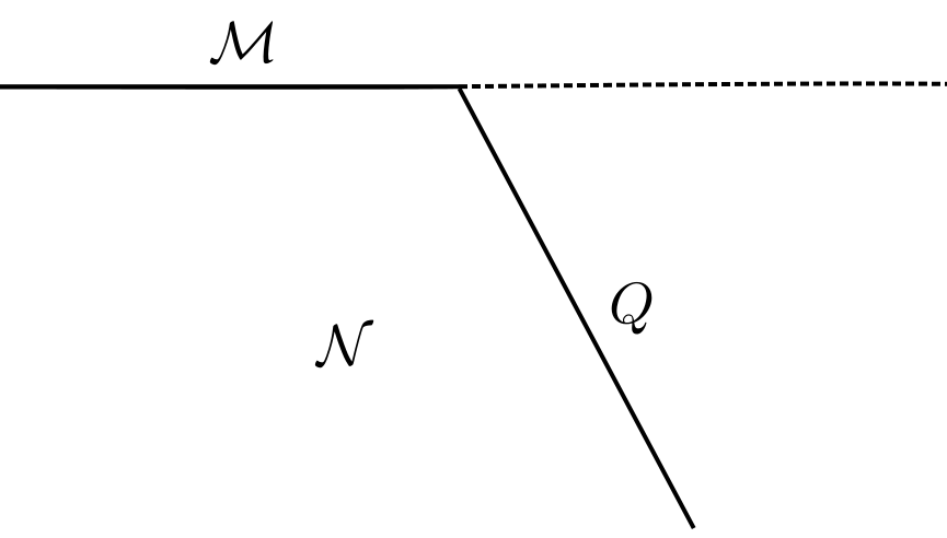
Figure 1: Holographic picture of a BCFT defined on the half-plane, $\mathcal{M}$.

One last point is that the boundary entropy of the BCFT is related to $T$. In particular, when $T=0$, the boundary entropy also vanishes.

2.3 The Yo-Yo String

The main reference here are [17] and [18]. The Yo-Yo solution is an example of a classical motion of an open string with finite momenta at end points. The main feature of such strings is that the end points move on light-like geodesics on a direction along the string itself. This is not compatible with any of the two allowed boundary conditions for open strings, namely the Dirichlet and Neumann boundary conditions. Still, they can be found as certain limits of allowed string configurations and hence should be considered as part of the classical theory.

In flat space, one can write solutions that interpolate between the Yo-Yo and the Regge solutions, the latter being an open string which rotates as a rod with a constant angular velocity. Such solutions satisfy the Neumann boundary conditions at ends and describes open strings that while rotating, their size changes between two positive numbers $l_{1}\geq l_{2}>0$. At any instant of time, the string is a straight line.

The Regge limit is when $l_{1}=l_{2}$. The other limit, Yo-Yo limit, is when $l_{2}\rightarrow 0$. In the Yo-Yo limit the Neumann boundary condition breaks down and for the energy of the string to be conserved one has to add a boundary term to the usual string action. The whole process can be generalised to arbitrary curved backgrounds [18].

In theories where open strings are not allowed, one can produce closed strings with the same above features. This amounts to attaching two open strings at end points and produce a closed string, folded back on itself, which, at any instant of time looks like a straight line. The important difference is that the open string ends are now replaced by the folding points which do not have to satisfy the open string boundary conditions. In the Yo-Yo limit, we will no longer need the additional boundary term and each half of the closed string provides the other half with the required boundary conditions. Therefore one has valid classical solutions of strings which carry momentum at the folding points. In the AdS background, these configurations are special cases of the rotating folded strings which were studied in [19], when the angular momentum is zero. The configurations are uniquely specified by a single number, the total length of the string or equivalently the total energy.

The solution of our interest in this work is the folded closed string in AdS₃ in coordinates (2.6). Working out the details (look at [18]) one finds that the folding points move on the trajectory $z=t$. Choosing the direction $z$ to parameterize this trajectory, one finds that the momentum of the folding point evolves as

$$\dot{p}_{t}=-\frac{TL^{2}}{4\pi G_{N}}\frac{1}{z^{2}}\ ,$$ (2.10)

where dot stands for differentiation with respect to $z$. One can state the initial value of $p_{t}$ in terms of the total energy of the string, $E$, which is $p_{t}(0)=-E/2$. Therefore one finds

$$p_{t}=-\frac{E}{2}+\frac{TL^{2}}{4\pi G_{N}}\frac{1}{z}\ .$$ (2.11)

Using this relation one can find the point where the folding point changes direction

$$z_{*}=\frac{TL^{2}}{2\pi G_{N}E}\ .$$ (2.12)

This is called the “snapback” point and is the closest the folding point can get to the boundary at $z=0$. This relation will find special significance in next section when we propose our holographic model for local quench.

2.4 Quench By Holography

There have been a number of attempts to describe local quench by holography, [23], [24] and [25]. see also [26]-[32]. Here we mention two of these works which are of more relevance to ours.

The first one is [23]. The process that is studied in this work is when a CFT undergoes a localized excitation. The excitation spreads throughout the system and changes the original state. The holographic model that [23] proposes for this process is to consider a massive particle which is falling freely in the AdS spacetime. As a result, the geometry in the bulk will be affected and the state of the system changes in time. Of particular interest is to compute the time dependence of EE for various subspaces. This is achieved by applying the RT prescription to the backreacted geometry and finding the corresponding minimal hypersurfaces in the bulk. In the case of AdS₃ the calculations can be done analytically. The results are in general agreement with expectations from field theory calculations.

The second work we mention here is [24], see also [25]. This reference makes a parallel computation of section(2.1) in the bulk. In particular, the bulk version of the map (2.1) is introduced and the field theory correlation functions of the twist operator are calculated by the usual RT curves in the bulk. The results thus obtained reproduce the field theory calculations of [7] correctly.

In the next section we propose another model for local quench when two CFT’s on semi-infinite lines are joined together. Our model considers each of the original BCFT’s in terms of their dual descriptions through the AdS/BCFT correspondence. Local quench occurs when the two extensions of the field theory boundaries, i.e., the $Q$ surfaces mentioned in (2.2) detach from the boundary and attach to one another. Their subsequent evolution in bulk determines the time dependence of the process. In this work we only consider BCFT’s with a zero boundary entropy. Extension to a general case is postponed to future works.

3 Local Quench By AdS/BCFT and Yo-Yo String

Consider a CFT living on a semi-infinite line $\mathcal{M}$ with $x<0$. The dual description will be the one depicted in figure (1). The $Q$ surface is determined by equations (2.8) and (2.9). Specify to the situation when the tension on $Q$ is zero. In the field theory language this means that the boundary entropy for this system is zero.

A key observation is that for $T=0$, the surface $Q$ is simply the world sheet of an open string which satisfies the classical equations of motion for a bosonic Polyakov string. The string attaches the boundary at $z=0$ with the usual Neumann boundary condition. The string, however, is tensionless; $\alpha^{\prime}\rightarrow\infty$. To see this, one can simply note that for $T=0$, the extrinsic curvature $\mathcal{K}$ of the surface $Q$ vanishes and hence it is a minimal surface. Classical solutions for Polyakov action are also nothing but minimal world sheets. The Neumann boundary condition is also obvious from (2.8) which gives

$$\partial_{z}x_{Q}|_{z=0}=0\ \ \ \ \ \text{when}\ \ \ T=0\ .$$ (3.1)

Now consider an identical field theory which lives on the semi-infinite line $\tilde{\mathcal{M}}$ with $x>0$. Again the same situation holds as above. Figure (2) shows the two systems together with $Q$ and $\tilde{Q}$ being the world sheets of tensionless Polyakov open strings

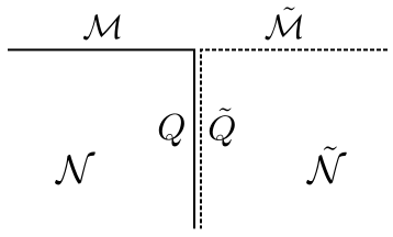
Figure 2: Two disconnected BCFT’s when $T\rightarrow 0$

Local quench occurs as a result of manipulations at and around the point $x=0$ which joins the two disconnected field theories into a single one. The question is what should be considered as the bulk version of these manipulations. Whatever these may be, they should occur in the UV part of the AdS space, around the $x=0$ point, which is a result of (rather) local manipulations around this point. It should ultimately result in the removal of the partition between the initially separate systems. Mirroring the field theory process, this should happen in a time dependent manner which entangles the degrees of freedom of the two systems as time goes by until one ends up in the ground state of single system, consisting of the two. Since this state is the ground state of conformal field theory on a line, the dual geometry must be empty AdS space.

Our proposal is that the bulk version corresponds to detaching each of the open strings from the boundary and attaching the two ends together. This will produce a folded closed string that can now propagate in the bulk (see figure(3)). This propagation happens according to the classical equations of motion for the string and should eventually result in the removal of the string, or its shrinking to a point, such that we are left with an empty AdS space at late times.

To find the subsequent motion of the string we note that once we attach the endpoints, we are left with a folded closed string which stretches along the radial coordinate in AdS with all of its points, including the folding point, at rest with zero momentum. This coincides with a tensionless yo-yo string at the snapback point which, in turn, is uniquely specified by its initial conditions. The dynamics will thus be governed by equations (2.10) and (2.11). The only remaining initial condition is the total energy of the string or the $z$ value of the folding point.

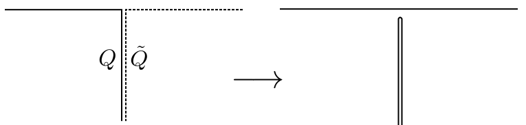
Figure 3: Holographic picture for local quench; appearance of a folded string

To find this last piece of information to determine the motion of the string we should properly define the tensionless limit of our yo-yo. Consulting equation (2.12), we see that a finite value for the snapback point $z_{*}$ can be find by

$$E\rightarrow 0\ ,\,\,\,\,\,T\rightarrow 0\ ,\,\,\,\,\,\lim_{T\rightarrow 0,E\rightarrow 0}z_{*}=\lim_{T\rightarrow 0,E\rightarrow 0}\frac{TL^{2}}{2\pi G_{N}E}\equiv\delta\ .$$ (3.2)

This is a reasonable limit once we remember what case of a quench we are studying. We are attaching two BCFT’s with zero boundary entropy. In such a case no energy is released or absorbed by quench [7]. Holographically this means that our AdS space never suffers back reactions by the folded string. This is also reflected in the $Q$ surfaces which are tensionless.

The last ingredient in our holographic picture for quench is to relate $\delta$ defined in (3.2) to field theory. A relevant question in the field theory side is how local the manipulations have been. In other words to what extent have the adjacent points around $x=0$ have been perturbed or excited as a result of quench. Let us assume that the process of attaching the two field theories has affected a region of size $\epsilon$.

We suggest that an interpretation of this length in terms of the bulk physics comes through the snapback point $z_{*}$ and hence $\delta$ (see figure (4))

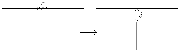
Figure 4: Regulators in boundary (Left) and bulk (Right).

A natural identification for our holographic picture will be then (fig.5)

$$\delta=\frac{1}{2}\ \epsilon\ .$$ (3.3)

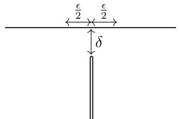
Figure 5: Identification of the regulators.

Let us see how this picture produces the general features of quench in the bulk. Dealing with zero boundary entropy for the initial BCFT’s, the whole process is governed by causal effects rather than energy transfer. In the field theory language this is a result of propagation of quasi-particles in both direction on the line which deliver the message of manipulations at $x=0$. These quasi-particles have an arbitrarily small energy.

In the bulk, the folded string falls freely away from the boundary into the bulk. The folding point falls on a light-like geodesic. The string has an arbitrarily small energy and does not back react on the geometry, again all that comes into play is the causal effects. The message of formation of the folded string propagates into the bulk along the light-cone depicted in figure (6).

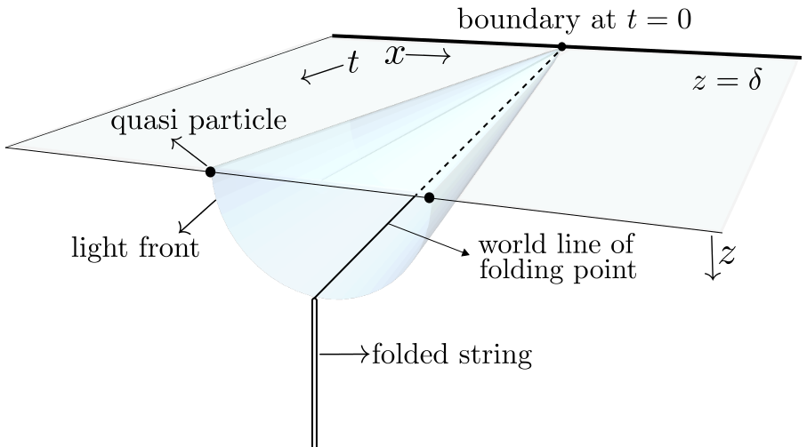
Figure 6: Holographic local quench: Light-cone and $\delta$ Vs. quasi-particles and $\epsilon$.

The light-cone divides bulk points into those who know of the manipulations and those who do not. The light front is identified as the bulk version of quasi-particles (6).

In the next section we will put our model to test by studying the time evolution of entanglement entropy of a single interval after quench.

4 Entanglement Entropy and Local Quench

The time dependence of entanglement entropy after quench will provide us with information of how the initial ground states of the disjoint BCFT’s will evolve into that of a single CFT on a line. Let us denote the entangling subregion by $A$ and its entanglement entropy by $S_{A}$. The complementary region and its entropy are denoted by $\bar{A}$ and $S_{\bar{A}}$ respectively. Since the entire system is in a pure state at any instant of time, $S_{A}=S_{\bar{A}}$ remains true at all times.

In field theory, one starts with the initial value for $S_{A}$. As the quasi-particles penetrate $A$, the entanglement pattern begins to change. One again arrives at a final value for $S_{A}$ as the quasi-particles exit $A$.

In the bulk side, one again starts with an initial condition. Denoting the endpoints of $A$ by $(x_{i},x_{j})$, the holographic value for $S_{A}$ is given by the RT curve through

$$S_{A}=\frac{\mathcal{A}(\gamma_{x_{i}x_{j}})}{4G_{N}}\,,$$ (4.1)

where $G_{N}$ is the newton constant, $\gamma_{x_{i}x_{j}}$ is the geodesic curve in the bulk that is homologous to $A$ and $\mathcal{A}(\gamma_{x_{i}x_{j}})$ is the length of $\gamma_{x_{i}x_{j}}$. As the light front of figure (6) intersects with $\gamma_{x_{i}x_{j}}$, it deforms the standard RT curve and changes $S_{A}$. Below, we propose how these deformations and modifications take place and try to justify them by physical intuitions and arguments.

The example we pick up for illustration is when $A$ is entirely inside one of the original BCFT’s. We follow the conventions of [7] to make comparisons immediate. The endpoints of $A$ are located at $\ell_{2}$ and $\ell_{1}$ with $\ell_{1}>\ell_{2}>0$. The two BCFT’s are joined at $x=t=0$. We first recall how the RT prescription works before quench and then propose how to modify it.

4.1 Entanglement entropy before the quench

To apply the standard RT prescription for holographic Entanglement Entropy one should find among all the curves that are homologous to the entangling region in the boundary the one that has the minimum length. In the case of a BCFT where additional boundaries exist both in the bulk and field theory sides the prescription has to be modified.

This amounts to considering two different types of curves, connected and disconnected. The former are the usual RT curves that end on the boundaries of the entangling region while the latter can end on the Q-surface in the bulk. Depending on the configuration of the entangling region and the Q-surface, the connected or disconnected pieces yield the minimum length and hence the EE.

To be more specific we consider the setup in the previous section where we have two BCFT’s with a common boundary and with a zero boundary entropy each. In the symmetrical situation at hand we find the introduction of ”Image Points” of special interest and use. These points make the application of the RT prescription more easy and systematic. We will later find that any modifications to the standard recipe will be facilitated by the image points.

One can see that the connected RT curves, $\gamma_{c}$, are those that start and end on (image) points whereas the disconnected curves, $\gamma_{d}$, correspond to those that have a point and an image on the ends. Below in figure (7), we have depicted the connected vs. disconnected RT curves.

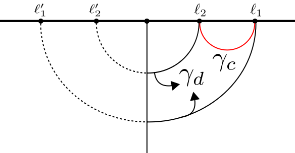
Figure 7: Connected vs. disconnected geodesic curves.

The recipe can then be summarized as

$$S_{EE}=\text{Min}\{\mathcal{A}(\gamma_{c})\,,\,\mathcal{A}(\gamma_{d})\}\,,$$ (4.2)

There are a number of comments worth mentioning. The problem of a single interval as the entangling region in a BCFT is in effect that of two disjoint intervals in a normal CFT. This is well expected as in a BCFT, the calculation of the two point function of twist operators will in effect be that of a four point function of operators inserted at points and their images, see for example [33]. In the holographic setup this corresponds to the curves that can end on image points.

It is well known that four point functions cannot be completely fixed by conformal symmetry completely. They depend also on the operator content of the theory. They, however, include a universal part which is fixed by symmetries. Using the notation of (2.1) we can find the correlation function of twist operators, $\sigma$ and $\tilde{\sigma}$, and thus the partition function of the replicated theory as follows

$$Z_{n}=\,\mathrm{Tr}\,\rho_{A}^{n}\propto\langle\sigma\tilde{\sigma}\text{(interval endpoints)}\rangle^{n}_{z}\sim\langle\sigma\tilde{\sigma}\text{(interval endpoints)}\sigma\tilde{\sigma}\text{(image points)}\rangle^{n}_{w}\,.$$ (4.3)

Consequently, we will have

$$Z_{n}=Z_{n}^{(u)}\,\widetilde{\mathcal{F}}_{n}(\{x\})\,,$$ (4.4)

where $Z_{n}^{(u)}$ represents the universal part of the replicated partition function, and $\widetilde{\mathcal{F}}_{n}(\{x\})$ stands for a non-universal function of cross-ratios which are shown by $\{x\}$ in sum.

However, as we will argue later, the important part for our purposes is the universal one. Using this technique the authors of [7] have computed the EE for various cases. For the most general case, i.e. for a single interval $A:[\ell_{2}>0,\ell_{1}>0]$ they have found

$$S_{A}=\frac{c}{6}\log\frac{(\ell_{1}-\ell_{2})^{2}}{(\ell_{1}+\ell_{2})^{2}}\frac{4\ell_{1}\ell_{2}}{a^{2}}\,.$$ (4.5)

To facilitate the following discussion, and also to make contact with the holographic description of EE, we rewrite the above relation as a sum of separate parts

$$S_{A}=S_{c}+S_{d}+S_{n}=\frac{c}{6}\log\frac{(\ell_{1}-\ell_{2})^{2}}{a^{2}}+\frac{c}{6}\log\frac{4\ell_{1}\ell_{2}}{a^{2}}+\frac{c}{6}\log\frac{a^{2}}{(\ell_{1}+\ell_{2})^{2}}\ ,$$ (4.6)

where the subscripts $c,d,n$ refer to connected, disconnected and negative contributions respectively. We recognize the first two contributions as corresponding to the familiar connected, $\gamma_{c}$, and disconnected, $\gamma_{d}$, RT curves. The negative contribution, however, although appearing in the universal part, has no counterpart amongst the RT curves.

In order to get an insight into this contribution to EE, consider a situation where one changes the length of the entangling region or its position with respect to the boundary smoothly. Interestingly, the negative contribution can make the transition between connected and disconnected pieces a smooth one. To see this we first consider the limit $\ell_{1}\gg\ell_{2}>0$ in (4.5). In this limit $\ell_{1}+\ell_{2}\sim\ell_{1}-\ell_{2}$ and the disconnected piece, $\gamma_{d}$, dominates. In the opposite limit $\ell_{2}\gg\ell_{1}-\ell_{2}>0$, we have $\ell_{1}\sim\ell_{2}$ and thus $(\ell_{1}+\ell_{2})^{2}\sim 4\ell_{1}\ell_{2}$ and therefore $\gamma_{c}$ survives.

Moving to the holographic description we find it natural to include the negative contribution in terms of geodesic curves specially since it appears in the universal part. This should be understood as our proposal for how to modify the RT prescription in case of multiple intervals as well as a single interval in presence of a boundary.

The holographic counterparts of these contributions can easily be identified as two intersecting curves between points and their images. Denoting the image points by $\tilde{\ell_{1}}$ and $\tilde{\ell_{2}}$ the negative contribution can be produced by

$$\text{Negative contribution}:\frac{1}{2}\{\mathcal{A}(\gamma_{\ell_{1}\ell^{\prime}_{2}})+\mathcal{A}(\gamma_{\ell^{\prime}_{1}\ell_{2}})\}\,.$$ (4.7)

So in summary, we have proposed the following prescription for computing the entanglement entropy holographically, before quench

$$\mathcal{A}_{0}=\frac{1}{2}\{\mathcal{A}(\gamma_{\ell_{1}\ell_{2}})+\mathcal{A}(\gamma_{\ell^{\prime}_{1}\ell^{\prime}_{2}})\}+\frac{1}{2}\mathcal{A}(\gamma_{\ell_{1}\ell^{\prime}_{1}})+\frac{1}{2}\mathcal{A}(\gamma_{\ell_{2}\ell^{\prime}_{2}})-\frac{1}{2}\{\mathcal{A}(\gamma_{\ell_{1}\ell^{\prime}_{2}})+\mathcal{A}(\gamma_{\ell^{\prime}_{1}\ell_{2}})\}\ .$$ (4.8)

This coincides with the universal part of the field theory calculations, produces the connected and disconnected pieces in the appropriate limits and makes a transition between the limits possible. (4.8) should be considered as our proposal to correct/modify the standard recipe of (4.2).

We have intentionally separated the contributions from points and their images because, as we will see in the following, the modifications will treat them differently. In figure (8) we have shown the positive and negative contributions by black and red curves, respectively.

In sum we believe that (4.8) should be considered as the holographic prescription for computing the EE which sums two connected and disconnected pieces and includes the negative contribution. We would like to emphasize again that it is somehow different from (4.2), since in the latter, among the connected and disconnected pieces only the minimal one is taken into account.

Incidentally we recently became aware of [34] in which the authors have computed the EE for two disconnected subregions in $1+1$ dimensions. Interestingly, our result is in a complete agreement with what they have found and hence this would provide a further support for what we have proposed in eq.(4.8).

The above prescription will give us the following value for $S_{A}$

$$S_{A}(t<\ell_{2})=\frac{c}{6}\log\frac{(\ell_{1}-\ell_{2})^{2}}{(\ell_{1}+\ell_{2})^{2}}\frac{4\ell_{1}\ell_{2}}{a^{2}}\,,$$ (4.9)

where $c$ is the central charge of the CFT and $a$ is a regularization parameter which is the lower bound for the coordinate $z$ (look at Appendix (A) for details).

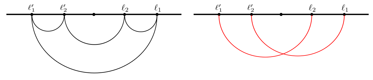
Figure 8: Positive (Left) vs. Negative (Right) contributions.

4.2 Entanglement entropy after the quench

As stated before the main reference for field theory results is [1]. As we discussed before, in their calculations universal as well as non-universal parts appear. The latter are in general, functions of cross ratios. In some limits these contributions become negligible.

As argued by the authors of [1], the EE after quench is well approximated by the universal parts. The non-universal parts are suppressed except at special times when the quasi-particles pass through the boundaries of the entangling region, i.e., the end points of the intervals.

In the following where we propose how the RT curves must be deformed and modified after quench, we are able to produce the universal contributions to EE as a function of time. This means that at times when the non-universal parts become important, further modifications should be introduced. Whatever these might be, they should depend on the specific CFT under study.

In the limit of a large central charge where classical gravity is believed to capture universal features of CFT’s, one may naturally expect that non-universal contributions will not have a simple gravitational description.

First step is to motivate the modification we formerly pointed out and to do that we note that the complementary region to $A$, denoted by $\bar{A}$, changes in time. At early times when $A$ has not yet received the message of quench, its reduced density matrix $\rho_{A}$ is unaffected and hence $S_{A}$ remains unchanged. After the quasi-particle has penetrated $A$ (say at time $t=t_{*}$), part of the region, denoted by $\alpha\subset A$, receives the message and the entanglement pattern begins to change. This continues until the quasi-particle exits the interval when $S_{A}$ assumes its steady state value. We are only interested in the intermediate times $\ell_{2}<t<\ell_{1}$ in the following.

Entanglement entropy changes by two competing contributions; one that decreases $S_{A}$ and one that increases it. Some of the existing entanglements disappear and some new ones form. In other words, the entanglement between $A$ and $\bar{A}(t<t_{*})$ transfers to that between $A$ and $\bar{A}(t>t_{*})$.

As the quasi-particle pair travel in both directions, the degrees of freedom in $\alpha$ find new counterparts to entangle with. These are those degrees of freedom which have been swept by the pair. This in turn transfers part of entanglement between $A$ and $\bar{A}(t<t_{*})$ to $\alpha$ and $\bar{A}(t>t_{*})$.

The decreasing contribution can be best understood by focusing on the image point $\ell^{\prime}_{2}$. Note that quasi-particles deal with points and their images differently. This is because the image points owe their existence to the boundary and as the boundary is removed the image points and their effects should be swept away. It is thus reasonable to assume that the point $\ell^{\prime}_{2}$ is swept off to left to $\tilde{\ell}^{\prime}_{2}$ (see figure (9)) as the quasi-particle passes through it.

Turning to the holographic description, this will modify some of the original RT curves. Out of the six contributions in (4.8), let us first focus on the four curves $\gamma_{\ell_{1}\ell_{2}},\gamma_{\ell^{\prime}_{1}\ell^{\prime}_{2}},\gamma_{\ell_{1}\ell^{\prime}_{2}}$ and $\gamma_{\ell_{2}\ell^{\prime}_{1}}$ and leave the remaining two for later. The shift of $\ell^{\prime}_{2}\rightarrow\tilde{\ell}^{\prime}_{2}$ decreases the positive contribution of $\mathcal{A}(\gamma_{\ell^{\prime}_{1}\ell^{\prime}_{2}})\rightarrow\mathcal{A}(\gamma_{\ell^{\prime}_{1}\tilde{\ell}^{\prime}_{2}})$ and increases the negative contribution of $\mathcal{A}(\gamma_{\ell_{1}\ell^{\prime}_{2}})\rightarrow\mathcal{A}(\gamma_{\ell_{1}\tilde{\ell}^{\prime}_{2}})$ while leaves the two parts $\mathcal{A}(\gamma_{\ell_{1}\ell_{2}})$ and $\mathcal{A}(\gamma_{\ell_{2}\ell^{\prime}_{1}})$ unchanged.

The modified curves, up to now, are summarized in figure(9).

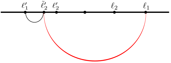
Figure 9: Image point moved to left. This decreases entanglement.

Using RT formula for the deformed curves and noting that $\tilde{\ell}^{\prime}_{2}=t$, we have

$$\mathcal{A}(\gamma_{\ell^{\prime}_{1}\tilde{\ell}^{\prime}_{2}})=\frac{c}{6}\log\frac{(\ell_{1}-t)^{2}}{a^{2}}\ ,\,\,\,\,\,\mathcal{A}(\gamma_{\ell_{1}\tilde{\ell}^{\prime}_{2}})=\frac{c}{6}\log\frac{(\ell_{1}+t)^{2}}{a^{2}}\ .$$ (4.10)

The contribution of the mentioned four curves appears in the following combination

$$\frac{1}{2}\{\mathcal{A}(\gamma_{\ell_{1}\ell_{2}})+\mathcal{A}(\gamma_{\ell^{\prime}_{1}\tilde{\ell}^{\prime}_{2}})\}-\frac{1}{2}\{\mathcal{A}(\gamma_{\ell_{1}\tilde{\ell}^{\prime}_{2}})+\mathcal{A}(\gamma_{\ell^{\prime}_{1}\ell_{2}})\}\ ,$$ (4.11)

Quite interestingly, this combination can be depicted in terms of geodesic curves in a very suggestive way. This is shown in figure (10) and illustrates the causal nature of deformations in the RT curves as a result of quench

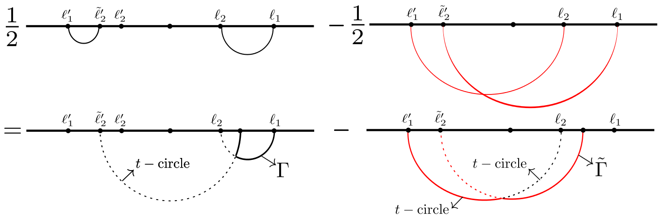
Figure 10: RT curves deformed by light-cone: $\Gamma$ and $\tilde{\Gamma}$.

The $t$-circle in this figure is the light front at time $t$. This picture motivates us to propose that the light-cone of the falling folded string deforms the RT curves as shown in figure(10). We call the combination in (4.11) as the decreasing contribution and denote it by $S_{D}$. In figure (10) we have introduced two new curves, $\Gamma$ and $\tilde{\Gamma}$. In figure(11) we give a better illustration for the former.

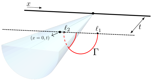
Figure 11: Deformed RT curve.

In calculating the lengths of the new curves we come across pieces that arrive at the boundary along the light front. We should note that along such pieces the minimal value for $z$, which appears as a limit in integrals, must be set equal to $\delta$, the light-cone regulator. Straightforward calculations lead to

$$\mathcal{A}(\Gamma)=\frac{c}{6}\ \log\frac{2t}{\delta}\ \frac{\ell_{1}-\ell_{2}}{a}\ \frac{\ell_{1}-t}{\ell_{2}+t}\ ,\ \ \ \\ \mathcal{A}(\tilde{\Gamma})=\frac{c}{6}\ \log\frac{2t}{\delta}\ \frac{\ell_{1}+\ell_{2}}{a}\ \frac{\ell_{1}+t}{\ell_{2}+t}\ ,$$ (4.12)

and the net contribution of the decreasing part, $S_{D}$, will be

$$S_{D}=\mathcal{A}(\Gamma)-\mathcal{A}(\tilde{\Gamma})=\frac{c}{6}\ \log\frac{\ell_{1}-\ell_{2}}{\ell_{1}+\ell_{2}}\ \frac{\ell_{1}-t}{\ell_{1}+t}\ .$$ (4.13)

As one can see, $a$ and $\delta$ dependence cancel out. The situation is of course different once we study the increasing contribution of $S_{A}$.

Up to now we have addressed four of the initial RT curves and their possible modifications after quench. We now turn to the remaining two. Of these, $\gamma_{\ell_{1}\ell^{\prime}_{1}}$ is unaffected through the whole process as it is outside the light cone. The other one however, $\gamma_{\ell_{2}\ell^{\prime}_{2}}$, will get modified in the increasing contribution to the EE. This contribution, as stated before, is a result of the new entanglements that the subset $\alpha$ finds with those degrees of freedom that have already received the quench message. In figure (12) we suggest how to modify RT for this contribution.

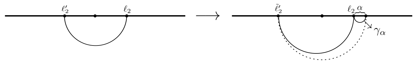
Figure 12: Modifications to RT for the increasing contribution to entanglement.

In the right hand side picture of figure (12), where we have proposed modifications to RT, the curve on the left is the deformation of the previously existing curve $\gamma_{\ell_{2}\ell^{\prime}_{2}}$. As the light front passes through the image point $\ell^{\prime}_{2}$, it sweeps away the image and drags the curve to $\tilde{\ell}^{\prime}_{2}$.

We also propose that a new piece of curve, henceforth denoted by $\gamma_{\alpha}$, forms between $\ell_{2}$ and the light front on the right. This is to account for the new entanglements that are formed between $\alpha$ and the interval $(\ell_{2},\tilde{\ell}^{\prime}_{2})$. Out of all the curves that we consider to find $S_{A}$, this is the only one that is produced during the process unlike the other ones which are deformations of initial curves. In this sense the appearance of $\gamma_{\alpha}$ in our recipe is not as natural and satisfactory as the deformed curves we have proposed. In particular, and as we will see below, we need to put a factor of $1/2$ in front of $\mathcal{A}(\gamma_{\alpha})$ to produce the correct results. This factor is a result of boundaries in the problem and we are aware that after quench when $\gamma_{\alpha}$ forms no boundaries exist. It would be much more satisfactory if one could predict and motivate the formation of this new curve by field theory arguments. Unfortunately at the moment we do not have a compelling argument in favour of this part of our proposal except that we have tested it in various cases when we change the relative position of the boundary and the interval and we have always produced the correct results. In particular we have applied the recipe to the cases of $\ell_{1}\rightarrow\infty,\ell_{2}=0$ and $\ell_{2}<0$ and found full agreement with field theory. We hope to report progress in this line in future works.

In any case for the curves in figure (12) one calculates

$$\mathcal{A}(\gamma_{\ell_{2}\tilde{\ell}^{\prime}_{2}})=\frac{c}{6}\log\frac{(t+\ell_{2})^{2}}{a\delta}\ ,\mathcal{A}(\gamma_{\alpha})=\frac{c}{6}\log\frac{(t-\ell_{2})^{2}}{a\delta}\ ,$$ (4.14)

which gives the increasing contribution, $S_{I}$ as

$$S_{I}=\frac{1}{2}\mathcal{A}(\gamma_{\ell_{2}\tilde{\ell}^{\prime}_{2}})+\frac{1}{2}\mathcal{A}(\gamma_{\alpha})=\frac{c}{6}\log\frac{t^{2}-\ell_{2}^{2}}{a\delta}\ .$$ (4.15)

Putting everything together, we end up with

$$S_{A}=S_{D}+S_{I}+\frac{1}{2}\mathcal{A}(\gamma_{\ell_{1}\ell^{\prime}_{1}})=\frac{c}{6}\ \log\frac{\ell_{1}-\ell_{2}}{\ell_{1}+\ell_{2}}\ \frac{\ell_{1}-t}{\ell_{1}+t}\ \frac{t^{2}-\ell_{2}^{2}}{a\delta}\ \frac{2\ell_{1}}{a}\ .$$ (4.16)

Note that the last term is simply the only initial curve which has not been affected by the light front. If we now express the holographic light-cone regulator $\delta$ in terms of the field theory quench regulator $\epsilon$ through equation (3.3), we recover the field theory result of [7] in full agreement.

A last point worth mentioning is to see how the image points and their effects are totally erased as the boundary is removed. This is accomplished by the deformed curves. By the time the quasi-particle reaches $\ell^{\prime}_{1}$, that is when $\tilde{\ell}^{\prime}_{2}$ coincides with $\ell^{\prime}_{1}$, $\mathcal{A}(\gamma_{\ell^{\prime}_{1}\tilde{\ell}^{\prime}_{2}})$ tends to zero while the negative part due to $\mathcal{A}(\gamma_{\ell_{1}\tilde{\ell}^{\prime}_{2}})$ will be canceled by $\mathcal{A}(\gamma_{\ell_{1}\ell^{\prime}_{2}})$ which is one of the initial RT curves before quench. In addition, $\mathcal{A}(\gamma_{\ell_{2}\tilde{\ell}^{\prime}_{2}})$ will cancel the negative part $\mathcal{A}(\gamma_{\ell_{2}\ell^{\prime}_{1}})$ which had remained unchanged by the modifications in the increasing contribution.

In figure (13) we summarize our proposal for the deformation and modification of RT curves by the folded string light-cone.

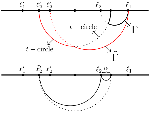
Figure 13: Summary of modifications to RT; Above (below) produces $S_{D}$($S_{I}$).

4.3 Interpretation of deformed RT curves

The deformed curves $\Gamma$ and $\tilde{\Gamma}$ suggest a very interesting interpretation. Recall the standard RT prescription for holographic EE. A very illuminating interpretation of this proposal was introduced in reference [35] where the EE of a spherical region was explained in terms of the statistical entropy of a related system in finite temperature. The latter system has a gravitational dual which is a topological black hole.

As was shown in [35], RT curve turns out to be the horizon of the topological black hole and the bulk points which are enclosed by this curve are the degrees of freedom outside the horizon. This suggests that the reduced density matrix of the entangling region can be described holographically by the bulk points enclosed by the RT curve and that the length of the curve gives an account for the number of states.

Now consider the RT curve $\gamma_{\ell_{1}\ell_{2}}$ which can be interpreted as above. As the light-front of quench intersects this curve it deforms it into $\Gamma$. This curve encloses only those points in the bulk which are still unaware of quench. The length of this curve can be interpreted as how the original EE of the region is decreasing. The new entanglements that are formed are accounted for by the points in the bulk that are inside the light-cone. This, in principle, should be responsible for the new curve $\gamma_{\alpha}$.

Finally, one should note that there are other possibilities for the entangling interval. In all cases our proposal for deformation of RT curves works perfectly and the results are in complete agreement with field theory.

5 Discussion

In this work we have proposed a holographic model for local quench in $1+1$ dimensional CFT. Local quench is a result of joining two identical BCFT’s living on semi-infinite lines. We have assumed that the initial theories have a zero boundary entropy.

Using AdS/BCFT our starting point in bulk is described by two halves of AdS₃ which are bounded by the boundary at $z=0$ on the one hand and a surface $Q$ (and $\tilde{Q}$) on the other. We observe that for a zero boundary entropy the surfaces $Q$ and $\tilde{Q}$ coincide with the tensionless Polyakov strings which end at the boundary with a Neumann boundary condition.

Local quench is described holographically when the open strings detach from boundary and form a closed string in the bulk. The resulting closed string is a folded tensionless string whose dynamics is given by the so called ”Yo-Yo” solution. In particular the tip of the folded string falls away from the boundary on a light-like geodesic. Being tensionless, the string does not back react on the geometry.

On the field theory side, the process of quench has a short distance regulator which determines the locality of the process. Also, the quasi-particles which are produced by local manipulations propagate through the system and produce the time dependence after quench. In our holographic setup we introduce the geometric counterparts of these features.

The short distance regulator naturally appears as the minimal distance between the tip of the folded string and the boundary. We give an interpretation of this regulator in terms of that for quench. As the folding point travels on a light-like geodesic, a light-cone propagates throughout the bulk. The origin of this cone is the space-time point that the closed string has formed. The light-front is thus interpreted as the bulk extension of the field theory quasi-particles.

We use the holographic model to calculate time dependent entanglement entropy after quench. We propose how the light-cone deforms standard RT curves and thus the EE. We find full agreement with field theory results.

Dealing with a time dependent process, it is more natural to apply the time dependent prescription to calculate holographic EE according to [36]. Working in constant time slices we avoid possible complications in this paper but it would be nice to derive same results by the mentioned proposal.

A possibly interesting generalization of this work is to study the same problem in the global coordinates. This would correspond to a process of joining two CFT’s on intervals at the two ends and create a CFT on a circle. The bulk picture will be a closed string that evolves in space.

A more challenging extension of this work is to study local quench when the boundary entropy is nonzero. The bulk surfaces $Q$ will not be tensionless in this case. One should find the dynamics of the surfaces in the bulk and should also take into account the back reaction on the geometry. As pointed out in [7], one expects that in a unitary evolution of the system, the original excess of energy will not dissipate and hence the system will always have a memory of the initial condition. This feature was absent in the present work as no energy excess existed in the first place. This problem is currently under investigation.

Appendix

Appendix A Geodesics in AdS₃

In this appendix we will find geodesics in $AdS_{3}$ and calculate their length.

Consider the following parametrization for a geodesic, $\gamma_{x_{1}x_{2}}$, in AdS₃, (2.6)

$$t=0\,\,\,\,\,,\,\,\,\,\,x_{\gamma}=x_{\gamma}(z)\,.$$ (A.1)

which is a co-dimension two hypersurface whose induced metric reads

$$ds_{ind}^{2}=\frac{L^{2}}{z^{2}}\left(1+{x^{\prime}_{\gamma}}^{2}\right)dz^{2}\,.$$ (A.2)

Hence, one can evaluate the length of the curve as

$$\mathcal{A}=2\int dz\frac{L}{z}\sqrt{1+{x^{\prime}_{\gamma}}^{2}}\,.$$ (A.3)

The integrand can be considered as a Lagrangian which does not explicitly depend on variable $x_{\gamma}$

$$\mathcal{L}=\mathcal{L}[{x^{\prime}_{\gamma}}(z)]\equiv\frac{L}{z}\sqrt{1+{x^{\prime}_{\gamma}}^{2}}\,,$$ (A.4)

therefore the equation of motion fixes the profile of the curve as

$$\frac{\partial\mathcal{L}}{\partial{x^{\prime}_{\gamma}}}=\text{const.}\rightarrow{x^{\prime}_{\gamma}}(z)=\frac{z}{\sqrt{z_{0}^{2}-z^{2}}}\,,$$ (A.5)

where $z_{0}$ is the turning point at which ${x^{\prime}_{\gamma}}\rightarrow\infty$.
Substituting this profile in (A.3) and performing the integral we arrive at

$$\mathcal{A}=2\left(-L\log\frac{z_{0}+\sqrt{z_{0}^{2}-z^{2}}}{z}-L\log z_{0}\right)\Bigg{|}_{a}^{z_{0}}=2L\log\left(\frac{2z_{0}}{a}\right),$$ (A.6)

where $a$, represents the cut-off of the radial direction and $z_{0}=\frac{1}{2}|x_{1}-x_{2}|$.

References

- [1] P.Calabrese,J. Cardy “Time Dependence of Correlation Functions Following a Quantum Quench” Physical Review Letters, vol. 96, Issue 13, id. 136801 arXiv:cond-mat/0601225
- [2] P. Calabrese and J. Cardy, “Quantum Quenches in Extended Systems,” J. Stat. Mech. 0706, P06008 (2007) [arXiv:0704.1880 [cond-mat.stat-mech]].
- [3] P. Calabrese and J. Cardy, “Quantum quench in interacting field theory: A Self-consistent approximation,” Phys. Rev. B 81 (2010) 134305 [arXiv:1002.0167 [quant-ph]].
- [4] J. M. Maldacena, “The Large N limit of superconformal field theories and supergravity,” Adv. Theor. Math. Phys. 2, 231 (1998) [hep-th/9711200].
- [5] E. Witten, “Anti-de Sitter space and holography,” Adv. Theor. Math. Phys. 2, 253 (1998) [hep-th/9802150].
- [6] O. Aharony, S. S. Gubser, J. M. Maldacena, H. Ooguri and Y. Oz, “Large N field theories, string theory and gravity,” Phys. Rept. 323 (2000) 183 [hep-th/9905111].
- [7] P. Calabrese and J. L. Cardy, “Entanglement and correlation functions following a local quench: a conformal field theory approach,“ J. Stat. Mech. P10004(2007) P10004 [cond-mat/0708.3750].
- [8] Eisler, V. and Peschel, I., “ Evolution of entanglement after a local quench,“ J. Stat. Mech. (2007) P06005, cond-mat/0703379;
- [9] , Eisler, V. and Karevski, D. and Platini, T. and Peschel, I. , “Entanglement evolution after connecting finite to infinite quantum chains“, J. Stat. Mech. (2008) P01023, arXiv:0711.0289.
- [10] Divakaran, U. and Iglói, F. and Rieger, H., “Non-equilibrium quantum dynamics after local quenches, Journal of Statistical Mechanics: Theory and Experiment, doi = 10.1088/1742-5468/2011/10/P10027,
- [11] P. Calabrese and J. Cardy, “Entanglement entropy and conformal field theory,” J. Phys. A 42, 504005 (2009) [arXiv:0905.4013 [cond-mat.stat-mech]].
- [12] T. Hartman and J. Maldacena, “Time Evolution of Entanglement Entropy from Black Hole Interiors,” JHEP 1305, 014 (2013) [arXiv:1303.1080 [hep-th]].
- [13] J. Aparicio and E. Lopez, “Evolution of Two-Point Functions from Holography,” JHEP 1112, 082 (2011) [arXiv:1109.3571 [hep-th]].
- [14] T. Albash and C. V. Johnson, “Evolution of Holographic Entanglement Entropy after Thermal and Electromagnetic Quenches,” New J. Phys. 13, 045017 (2011) [arXiv:1008.3027 [hep-th]].
- [15] T. Takayanagi, “Holographic Dual of BCFT,” Phys. Rev. Lett. 107, 101602 (2011) [arXiv:1105.5165 [hep-th]].
- [16] M. Fujita, T. Takayanagi and E. Tonni, “Aspects of AdS/BCFT,” JHEP 1111, 043 (2011) [arXiv:1108.5152 [hep-th]].
- [17] W. A. Bardeen, I. Bars, A. J. Hanson and R. D. Peccei, “A Study of the Longitudinal Kink Modes of the String,” Phys. Rev. D 13, 2364 (1976).
- [18] A. Ficnar and S. S. Gubser, “Finite momentum at string endpoints,” Phys. Rev. D 89, 026002 (2014) [arXiv:1306.6648 [hep-th]].
- [19] S. S. Gubser, I. R. Klebanov and A. M. Polyakov, “A Semiclassical limit of the gauge / string correspondence,” Nucl. Phys. B 636, 99 (2002) [hep-th/0204051].
- [20] S. Ryu and T. Takayanagi, “Holographic derivation of entanglement entropy from AdS/CFT,” Phys. Rev. Lett. 96, 181602 (2006) [hep-th/0603001].
- [21] T. Nishioka, S. Ryu and T. Takayanagi, “Holographic Entanglement Entropy: An Overview,” J. Phys. A 42, 504008 (2009) [arXiv:0905.0932 [hep-th]].
- [22] S. Ryu and T. Takayanagi, “Aspects of Holographic Entanglement Entropy,” JHEP 0608, 045 (2006) [hep-th/0605073].
- [23] M. Nozaki, T. Numasawa and T. Takayanagi, “Holographic Local Quenches and Entanglement Density,” JHEP 1305, 080 (2013) [arXiv:1302.5703 [hep-th]].
- [24] T. Ugajin, “Two dimensional quantum quenches and holography,” arXiv:1311.2562 [hep-th].
- [25] C. T. Asplund and A. Bernamonti, “Mutual information after a local quench in conformal field theory,” Phys. Rev. D 89, 066015 (2014) [arXiv:1311.4173 [hep-th]].
- [26] P. Basu and S. R. Das, “Quantum Quench across a Holographic Critical Point,” JHEP 1201, 103 (2012) [arXiv:1109.3909 [hep-th]].
- [27] S. R. Das, “Holographic Quantum Quench,” J. Phys. Conf. Ser. 343, 012027 (2012) [arXiv:1111.7275 [hep-th]].
- [28] A. Buchel, L. Lehner and R. C. Myers, “Thermal quenches in N=2* plasmas,” JHEP 1208, 049 (2012) [arXiv:1206.6785 [hep-th]].
- [29] P. Basu, D. Das, S. R. Das and T. Nishioka, “Quantum Quench Across a Zero Temperature Holographic Superfluid Transition,” JHEP 1303, 146 (2013) [arXiv:1211.7076 [hep-th]].
- [30] A. Buchel, L. Lehner, R. C. Myers and A. van Niekerk, “Quantum quenches of holographic plasmas,” JHEP 1305, 067 (2013) [arXiv:1302.2924 [hep-th]].
- [31] J. F. Pedraza, “Evolution of nonlocal observables in an expanding boost-invariant plasma,” Phys. Rev. D 90, 046010 (2014) [arXiv:1405.1724 [hep-th]].
- [32] M. M. Roberts, “Time evolution of entanglement entropy from a pulse,” arXiv:1204.1982 [hep-th].
- [33] P. Di Francesco, P. Mathieu and D. Senechal, “Conformal field theory,” New York, USA: Springer (1997) 890 p
- [34] V. E. Hubeny and M. Rangamani, “Holographic entanglement entropy for disconnected regions,” JHEP 0803, 006 (2008) [arXiv:0711.4118 [hep-th]].
- [35] H. Casini, M. Huerta and R. C. Myers, “Towards a derivation of holographic entanglement entropy,” JHEP 1105, 036 (2011) [arXiv:1102.0440 [hep-th]].
- [36] V. E. Hubeny, M. Rangamani and T. Takayanagi, “A Covariant holographic entanglement entropy proposal,” JHEP 0707, 062 (2007) [arXiv:0705.0016 [hep-th]].