Democratic Neutrino Theory

Abstract

New theory of neutrino masses and mixing is introduced. This theory is based on a simple $S_{3}$ symmetric democratic neutrino mass matrix, and predicts the neutrino mass spectrum of normal ordering. Taking into account the matter effect and proper averaging of the oscillations, this theory agrees with the variety of atmospheric, solar and accelerator neutrino data. Moreover, the absolute scale of the neutrino masses $m\approx 0.03$ eV is determined in this theory, using the atmospheric neutrino oscillation data. In case of tiny perturbations in the democratic mass matrix only one this scale parameter $m$ allows to explain the mentioned above neutrino results, and the theory has huge predictive power.

I Introduction

The neutrinos were proposed by W. Pauli in 1930 Pauli:2000ak and first detected by C. Cowan and F. Reines in 1956 Cowan:1992xc . Later the solar neutrino deficit Davis:1968cp , the atmospheric neutrino oscillations Fukuda:1998mi , and other neutrino oscillation results PDG2012 have revealed that the neutrino masses are nonzero. However the questions about the absolute scale of their masses, their type (whether Dirac or Majorana), etc., still remain unanswered.

Besides the reactor Mention:2011rk , Gallium Giunti:2012tn ; Abdurashitov:2005tb and few other neutrino anomalies, the available neutrino data can be explained within the phenomenological model of three light neutrinos with two mass splittings (squared mass differences) of close scales: $\Delta m_{s}^{2}\sim 10^{-4}$ eV² and $\Delta m_{a}^{2}\sim 10^{-3}$ eV² PDG2012 . We call it the conventional neutrino theory (CNT). In case of Majorana (Dirac) neutrinos the masses and mixings are generically parametrized in CNT by 9 (7) free parameters: 3 masses, 3 mixing angles and 3 phases (1 phase).

In this paper we show that the variety of the neutrino data can be explained in a model with three Majorana neutrinos with simple $S_{3}$ symmetric (in the leading order) “democratic” mass matrix. This democratic neutrino theory (DNT), which was briefly presented in Ref. Zhuridov:2013ika , predicts the normal hierarchy of the neutrino mass spectrum, and allows to determine from the atmospheric neutrino data the absolute scale of the neutrino masses of $m\approx 0.03$ eV.

In the case of slightly perturbed democratic mass matrix, DNT has huge predictive power, and only one its parameter $m$ is enough to determine to a good precision the available oscillation data. However there is a single large mass splitting. If it governs the atmospheric neutrino oscillations than the second mass splitting is much less than $10^{-4}$ eV². For this reason we give up the interpretation of the data obtained by the KamLAND experiment Araki:2004mb ; Gando:2010aa ; Gando:2013nba in terms of the neutrino oscillations due to their mass splitting of order $10^{-4}$ eV², and provide a nonstandard explanation of the solar neutrino data. Also in the discussed case the neutrino mass matrix is essentially different from the tri-bimaximal one Wolfenstein:1978uw ; Fritzsch:1995dj ; Harrison:2002er ; Harrison:2002kp ; Xing:2002sw , which motivates us to use alternative explanation of several atmospheric and accelerator neutrino observables.

On the other hand, for relatively large deviation from $S_{3}$ symmetric mass matrix a standard interpretation of the neutrino data may come into play, while the predictive power is reduced.

In the next section DNT is introduced, and the neutrino masses and mixing are derived. Further we discuss the neutrino oscillations in section III and alternative explanations of the neutrino experimental data in the framework of DNT in section IV. Then we compare DNT with CNT in section V, discuss the predictions of DNT in section VI, and conclude.

II Democratic Masses and Mixing

A lowest order democratic quark mass matrix proportional to

$$\left(\begin{array}[]{ccc}1&1&1\\ 1&1&1\\ 1&1&1\par\end{array}\right)$$ (4)

was discussed in the context of $S_{3}(L)\times S_{3}(R)$ symmetry of massless quarks in the $SU(2)_{L}\times SU(2)_{R}\times U(1)$ gauge model in Ref. Harari:1978yi . Possible relation of this matrix to the leptonic mixing was investigated in Ref. Fritzsch:1995dj . The two $S_{3}(L)$ invariant mass matrixes for Majorana neutrinos

$$\left(\begin{array}[]{ccc}1&0&0\\ 0&1&0\\ 0&0&1\\ \end{array}\right),\qquad\left(\begin{array}[]{ccc}0&1&1\\ 1&0&1\\ 1&1&0\\ \end{array}\right)$$ (11)

were discussed in Ref. Fukugita:1998vn with focus on the first of them. The second of the matrices in Eq. (11) was considered in Ref. Nicolaidis:2013hxa in the context of brane models. In DNT we consider this matrix as the leading order neutrino mass matrix in usual low-energy $SU(3)_{color}\times U(1)_{em}$ theory. Then we add either sizable (of order few %) or tiny (orders of magnitude less than 1%) perturbations. These two cases require different explanation of the neutrino data, see the following.

II.1 DNT to the leading order

Consider the mass term for three Majorana neutrinos

$$\mathcal{L}_{m}^{\nu}=-\frac{1}{2}\,\sum_{\alpha\beta}\bar{\nu}_{\alpha L}^{c}M_{\alpha\beta}\nu_{\beta L}+{\rm H.c.},$$ (12)

where $\alpha,\beta=e,\mu,\tau$ are the flavor indices, $c$ denotes charge conjugation, and

$$M=M_{0}+o(m)$$ (13)

is the neutrino mass matrix in the flavor basis, where

$$M_{0}=m\left(\begin{array}[]{ccc}0&1&1\\ 1&0&1\\ 1&1&0\\ \end{array}\right)$$ (17)

is a democratic mass matrix, which is invariant under the permutation group of three elements $S_{3}$ Harari:1978yi ; Fritzsch:1995dj ; Fukugita:1998vn ; Fujii:2002jw ; Mohapatra:1998rq ; Harrison:2003aw ; Nicolaidis:2013hxa , and is defined by the only mass scale parameter $m$. Possible perturbations to this leading order mass matrix are included in the little-o term $o(m)$ in Eq. (13), and they are discussed below. The eigenvectors of $M_{0}$ form the neutrino mixing matrix, which can be written as

$$U_{0}=\left(\begin{array}[]{ccc}\frac{1}{\sqrt{2}}&\frac{1}{\sqrt{6}}&\frac{1}{\sqrt{3}}\\ -\frac{1}{\sqrt{2}}&\frac{1}{\sqrt{6}}&\frac{1}{\sqrt{3}}\\ 0&-\frac{2}{\sqrt{6}}&\frac{1}{\sqrt{3}}\\ \end{array}\right),$$ (21)

and makes the transformation from flavor to mass basis as

$$\nu_{\alpha L}=\sum_{i=1,2,3}(U_{0})_{\alpha i}\nu_{iL},$$ (22)

where the subindex $0$ refers to the leading order approximation. The last column of $U_{0}$ corresponds to the larger eigenvalue of $M_{0}$, and the first row does not include zero to explain the solar neutrino data, see section IV.3. It is convenient to parametrize Eq. (21) using only two angles as

$$U_{0}=R_{12}(\tilde{\theta}_{12})\otimes R_{23}(\tilde{\theta}_{23})=\left(\begin{array}[]{ccc}c_{12}&s_{12}c_{23}&s_{12}s_{23}\\ -s_{12}&c_{12}c_{23}&c_{12}s_{23}\\ 0&-s_{23}&c_{23}\\ \end{array}\right)$$ (26)

where $c_{ij}\equiv\cos\tilde{\theta}_{ij}$, $s_{ij}\equiv\sin\tilde{\theta}_{ij}$, $\tilde{\theta}_{12}=45^{\circ}$, $\tilde{\theta}_{23}=\pi/2-\arctan(1/\sqrt{2})\approx 54.7^{\circ}$, and tilde denotes our parametrization. Notice that in Eq. (26) we used the opposite order of multiplication of the Euler rotation matrixes $R_{ij}$ with respect to the ordinary tri-bimaximal matrix Wolfenstein:1978uw ; Fritzsch:1995dj ; Harrison:2002er ; Harrison:2002kp ; Xing:2002sw .

In the case of standard parametrization of the neutrino mixing matrix PDG2012 ; Kayser:2002qs , Eq. (21) is reproduced by

$$U_{\text{standard}}=R_{23}(\theta_{23})\otimes R_{13}(\theta_{13})\otimes R_{12}(\theta_{12})$$ (27)

with $\theta_{12}=30^{\circ}$, $\theta_{23}=45^{\circ}$, $\theta_{13}=\arcsin(1/\sqrt{3})\approx 35.3^{\circ}$, and no $CP$ violating phases.

By diagonalizing the mass matrix $M_{0}$ with the matrix $U_{0}$ and expressing $\nu_{iL}$ through the Majorana spinors $\psi_{i}=\psi_{i}^{c}$ as

$$\nu_{iL}\equiv\frac{1}{2}(1-\gamma_{5})\psi_{i},$$ (28)

Eq. (12) can be rewritten as

$$\mathcal{L}_{m}^{\nu}=-\frac{1}{2}\,\sum_{i}s_{i}m_{i}\bar{\psi}_{i}\psi_{i},$$ (29)

where $m_{1}=m_{2}=m_{3}/2\equiv m$, and $s_{1}=s_{2}=-s_{3}=-1$ are the sign factors, which can be absorbed by the transformation $\psi_{j}\to i\gamma_{5}\psi_{j}^{\prime}$ ($j=1,2$). On relation of the sign factors to the neutrino $CP$ properties and mixing matrix see section 2.3.2 in Ref. Doi:1985dx and references therein. The resulting neutrino mass spectrum

$$\{m,m,2m\}$$ (30)

has normal ordering and two degenerate values, which results in the only mass splitting

$$\Delta m^{2}=3m^{2}.$$ (31)

II.2 Tiny perturbations

Similarly to the great variety of broken symmetries in nature, it is naturally that the degeneracy in Eq. (30) is violated by a small perturbations in Eq. (13). Suppose that these perturbations are tiny. This leads to a spectrum

$$\{m,m+\delta m,2m\},$$ (32)

where $0<\delta m/m$ measures the violation of “full democracy” (in section IV.3 we consider $\delta m/m\ll 10^{-4}$ for effective suppression of the respective oscillations in the Sun), and we ignore possible deviation in the eigenvalue $2m$ since this does not significantly effect the large neutrino mass splitting $\Delta m^{2}$. As a result, for the two splittings we have:

$$\Delta\mu^{2}\equiv(m+\delta m)^{2}-m^{2}\approx 2m\delta m$$ (33)

and $\Delta m^{2}=3m^{2}$. To consider the neutrino oscillations with reasonable accuracy the neutrino mixing matrix can be written as

$$U=\left(\begin{array}[]{ccc}\frac{1}{\sqrt{2}}&\frac{1}{\sqrt{6}}&\frac{1}{\sqrt{3}}\\ -\frac{1}{\sqrt{2}}&\frac{1}{\sqrt{6}}&\frac{1}{\sqrt{3}}\\ \lambda\left(\frac{\delta m}{m}\right)^{1/2}&-\frac{2}{\sqrt{6}}&\frac{1}{\sqrt{3}}\\ \end{array}\right),$$ (37)

where $\lambda$ is a constant of order one, and the deviations in nonzero elements are neglected since all these elements are large.

In section IV we show how atmospheric, solar and accelerator neutrino observables can be explained using only parameter $m$, neglecting small effects of other parameters.

II.3 Sizable perturbations

Consider the case of sizable perturbations in the mass matrix $M$, which lead to the spectrum

$$\{m+x_{1},m+x_{2},2m+x_{3}\},$$ (38)

where the deviations $x_{i}$ ($x_{2}>x_{1}$) can be written as

$$x_{i}=\xi_{i}\sqrt{\Delta m_{s}^{2}}$$ (39)

with the small, but essentially larger than $\delta m$ in Eq. (32), mass scale $\sqrt{\Delta m_{s}^{2}}$ ($0<\sqrt{\Delta m_{s}^{2}}\ll m$), and the dimensionless parameters $\xi_{i}$ of order unity ($\xi_{2}-\xi_{1}\ll 1$). Then the mass splitting

$$\Delta m_{a}^{2}\equiv(2m+x_{3})^{2}-(m+x_{1})^{2}$$ (40)

can be rewritten as

$$\Delta m_{a}^{2}=3m^{2}+\Delta m_{s}^{2}(\xi_{1}^{2}-\xi_{3}^{2})+{\cal O}\left(\frac{\Delta m_{s}^{4}}{\Delta m_{a}^{2}}\right),$$ (41)

and we end up with the spectrum

$$\left\{m_{1},\sqrt{m_{1}^{2}+\Delta m_{s}^{2}},\sqrt{m_{1}^{2}+\Delta m_{a}^{2}}\right\},$$ (42)

where $m_{1}\equiv m+x_{1}\approx\sqrt{\Delta m_{a}^{2}/3}$. The two splittings $\Delta m_{s}^{2}$ and $\Delta m_{a}^{2}$ may correspond to the ordinary solar and atmospheric neutrino mass splittings, respectively. (That is why we used this notation for them in Eqs. (39) and (40)). The neutrino mixing matrix has sizable corrections in relation to Eq. (21). In particular, the $U_{e3}$ element may be significantly smaller, and there may be essential $CP$ violation. Thereby, ordinary interpretation of the neutrino experimental data may be applied. However in the following sections we will concentrate on more interesting and predictive case of tiny perturbations, which requires an alternative explanation of the neutrino data.

In both cases of either tiny or sizable perturbations the neutrino mass spectrum has normal ordering, and the absolute neutrino mass scale is about $\sqrt{\Delta m^{2}/3}$. Using the atmospheric neutrino mass splitting $\Delta m_{a}^{2}=(2.06-2.67)\times 10^{-3}$ eV² (at 99.73% CL) PDG2012 , the absolute neutrino mass scale can be determined as

$$m\approx 0.03~{}\text{eV}.$$ (43)

III Neutrino oscillations

The probabilities of the flavor neutrino oscillations in vacuum can be written as

$$P_{\nu_{\alpha}\to\nu_{\beta}}(L,E)=\sum_{i}|U_{\alpha i}|^{2}|U_{\beta i}|^{2}$$

$$+2\sum_{i>j}|U_{\alpha i}^{*}U_{\beta i}U_{\alpha j}U_{\beta j}^{*}|\cos\left(2\pi\frac{L}{L_{ij}^{\text{osc}}}-\phi_{\beta\alpha;ij}\right),$$ (44)

where $L_{ij}^{\text{osc}}=4\pi E/\Delta m_{ij}^{2}$ is the oscillation length, and $\phi_{\beta\alpha;ij}=\arg(U_{\alpha i}^{*}U_{\beta i}U_{\alpha j}U_{\beta j}^{*})$ is the constant phase. Using the leading order democratic neutrino mass spectrum in Eq. (30) and mixing in Eq. (21) we have the “democratic” oscillation probabilities of the same size

$$P_{\nu_{\alpha}\to\nu_{\beta}}(L,E)=\frac{4}{9}\sin^{2}\left(\frac{\Delta m^{2}L}{4E}\right),$$ (45)

where $\beta\neq\alpha$.

In case of the spectrum of Eq. (32) the probabilities $P_{\nu_{\alpha}\to\nu_{\beta}}$ are slightly different from Eq. (45) due to the oscillation terms with $\Delta\mu^{2}$, while the results in Eq. (45) are reproduced in the limit $\Delta\mu^{2}L/4E\to 0$. In particular, for the electron neutrino survival probability we have

$$P_{\nu_{e}\to\nu_{e}}^{\text{survival}}=\frac{7}{18}+\frac{4}{9}\cos\left(\frac{\Delta m^{2}L}{2E}\right)+\frac{1}{6}\cos\left(\frac{\Delta\mu^{2}L}{2E}\right).$$ (46)

IV Neutrino experiments

In this section we discuss the explanation within DNT (in its case with tiny perturbations) of the data obtained by the neutrino experiments of several types.

IV.1 Atmospheric neutrinos

The atmospheric neutrino flux dominates by the neutrinos with the energies in the range $0.1-10^{2}$ GeV Giunti:2007ry . Correspondingly, for the oscillations due to $\Delta m^{2}\approx 3m^{2}$ with $m$ from Eq. (43) the oscillation length is in the range $10^{2}-10^{5}$ km, which is relevant for the terrestrial experiments. However the oscillations due to $\Delta\mu^{2}\ll 10^{-6}$ eV² can not be observed since their oscillation length $L_{12}^{\text{osc}}\gg 10^{5}$ km significantly exceeds the Earth diameter. For this reason, in DNT with tiny perturbations the atmospheric neutrino oscillation probabilities are well described by Eq. (45). Consider how this equation may explain the significant zenith-angle deficit of $\nu_{\mu}$ observed by the Super-Kamoikande (SK) detector Ashie:2005ik ; Ashie:2004mr ; Abe:2006fu . We remark that in CNT this deficit was interpreted as the 2-flavor $\nu_{\mu}\to\nu_{\tau}$ oscillations, taking into account the suppression of $\nu_{e}\to\nu_{\mu,\tau}$ oscillations by a small $\theta_{13}$.

In DNT this difference between the $e$-like and $\mu$-like event distributions in the SK can be explained by the 3-flavor oscillations in Eq. (45), taking into account the matter effect on $\nu_{e}$, which travel through the Earth. Indeed, for the electron neutrinos propagating in the matter with the electron number density $N_{e}$ the probability to oscillate into other flavor state can be written as PDG2012 ; Wolfenstein:1977ue ; Mikheev:1986gs ; Barger:1980tf

$$P_{m}(\nu_{e}\to\nu_{\alpha\neq e})=\sin^{2}2\theta_{m}\sin^{2}\left(\frac{\Delta M^{2}L}{4E}\right),$$ (47)

where

$$\sin 2\theta_{m}=\frac{\tan 2\theta}{\sqrt{\left(1-\frac{N_{e}}{N_{e}^{\rm res}}\right)^{2}+\tan^{2}2\theta}},$$ (48)

$$\Delta M^{2}=\Delta m^{2}\left[\left(1-\frac{N_{e}}{N_{e}^{\rm res}}\right)^{2}\cos^{2}2\theta+\sin^{2}2\theta\right]^{\frac{1}{2}},$$ (49)

and the Mikheyev-Smirnov-Wolfenstein (MSW) resonance density is given by

$$N_{e}^{\rm res} = \frac{\Delta m^{2}\cos 2\theta}{2\sqrt{2}EG_{\text{F}}}$$

$$\approx 6.56\times 10^{6}\,\frac{\Delta m^{2}[\text{eV}^{2}]}{E[\text{MeV}]}\cos 2\theta\quad\text{cm}^{-3}\,\text{N}_{\text{A}}$$

with $G_{\text{F}}$ and $\text{N}_{\text{A}}$ being Fermi constant and Avogadro number, respectively. In particular, for the atmospheric neutrinos with energies $E\sim 10$ GeV we have $N_{e}^{\rm res}\approx 1.15~{}\text{cm}^{-3}\,\text{N}_{\text{A}}$, and using the mean electron number density in the Earth core $\bar{N}_{e}^{c}\approx 5.4~{}\text{cm}^{-3}\,\text{N}_{\text{A}}$ PDG2012 ; Dziewonski:1981xy , we find

$$P_{m}(\nu_{e}\to\nu_{\alpha\neq e})=0.05\,\sin^{2}\left(2.8\frac{\Delta m^{2}L}{4E}\right),$$ (51)

which is significantly suppressed with respect to the vacuum oscillations in Eq. (45). Notice that the $\nu_{\mu}\leftrightarrow\nu_{\tau}$ oscillations in the matter of the Earth proceed practically as in vacuum due to approximate equality of the refraction indices PDG2012 .

IV.2 $\nu_{\mu}$ and $\bar{\nu}_{\mu}$ oscillations

The close to unity amplitude of the muon neutrino oscillations $A_{\mu}$ observed in the MINOS experiment Adamson:2013whj ; Adamson:2011ig is explained in DNT with tiny perturbations by the large oscillations of the muon neutrinos to both electron and tau neutrino flavors, and analogous for the antineutrinos. The matter effect plays a subdominant role for the beam neutrinos in the MINOS experiment in contrast to the nearly upward atmospheric neutrino events due to the shorter baseline $L=734$ km and relatively small matter density in the Earth crust $\bar{N}_{e}\approx 2~{}\text{cm}^{-3}\,\text{N}_{\text{A}}$. Neglecting the matter effect we have the probability

$$P(\nu_{\mu}\to\nu_{\alpha\neq\mu}) = P(\nu_{\mu}\to\nu_{e})+P(\nu_{\mu}\to\nu_{\tau})$$ (52)

$$\approx \frac{8}{9}\sin^{2}\left(\frac{\Delta m^{2}L}{4E}\right),$$

whose amplitude agrees with the MINOS result $\nobreak{A_{\mu}>0.890}$ ($\nobreak{A_{\mu}>0.83}$) at 90% CL for the muon (anti)neutrino oscillations, derived within 2-flavor approximation Adamson:2013whj . Reanalysis of the MINOS data taking into account the matter effect in the framework of 3-flavor democratic oscillations would even improve this agreement 1304.4870 .

We remark that in CNT $\nu_{\mu}\to\nu_{\tau}$ oscillations dominate in the muon neutrino disappearance in MINOS, and $A_{\mu}$ is considered as an amplitude $4|U_{\mu 3}|^{2}|U_{\tau 3}|^{2}$ of these $\nu_{\mu}\to\nu_{\tau}$ oscillations with close to maximal ($1/\sqrt{2}$) values of $|U_{\mu 3}|$ and $|U_{\tau 3}|$.

IV.3 Solar neutrinos

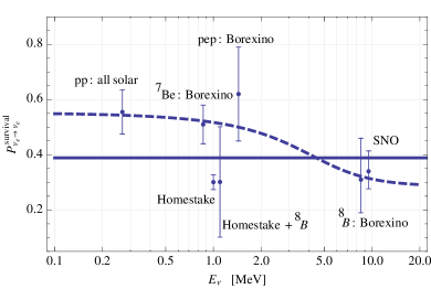
Figure 1: Survival probability for solar neutrinos $P_{ee}\equiv P_{\nu_{e}\to\nu_{e}}^{\text{survival}}$ vs. the neutrino energy. Solid (dashed) line represents the result of DNT with tiny perturbations (CNT).

Due to the combined effort of the fusion reactions, which produce the neutrinos in the core of the Sun

$$4p\to^{4}\text{He}+2e^{+}+2\nu_{e},$$ (53)

Sun is a source of the electron neutrinos. The observed flux of the solar neutrinos $\nu_{\odot}$ reveals a deficit with respect to the predictions of the standard solar model, which is known as the solar neutrino problem PDG2012 . In other words, the survival probability $P_{\nu_{e}\to\nu_{e}}^{\text{survival}}$ for solar neutrinos is suppressed with respect to unity, which is shown in Fig. 1 by the data points obtained by the Homestake Cleveland:1998nv , the SNO Aharmim:2005gt , the Borexino Bellini:2013lnn ; Calaprice:2012kc , and other solar neutrino experiments Giunti:2007ry . However part of the shown results for $P_{\nu_{e}\to\nu_{e}}^{\text{survival}}$ were determined by comparing the measured fluxes with standard solar model predictions Calaprice:2012kc .

In DNT with tiny perturbations the term in $P_{\nu_{e}\to\nu_{e}}^{\text{survival}}$, which is proportional to $\cos(\Delta m^{2}L/2E)$, is suppressed due to the averaging over the region of $\nu_{e}$ production in the Sun, similarly to CNT PDG2012 . On the other hand, the oscillations due to $\Delta\mu^{2}$ are strongly suppressed by the effect of solar matter if $\Delta\mu^{2}\ll 10^{-7}$. Hence from Eq. (46) we get an incoherent result

$$P_{\nu_{e}\to\nu_{e}}^{\text{survival}}=\frac{7}{18},$$ (54)

which is represented by the solid line in Fig. 1. This line comes to an agreement with the data in case of slightly less conservative error bars for the low energy data points. In fact, it is reasonable to reexamine these error bars since the low energy $\nu_{\odot}$ data still suffer from the Gallium anomaly Giunti:2012tn ; Abdurashitov:2005tb , the discrepancy between the Homestake and the Borexino results, effects of solar model calculations, etc. One example of such reexamination was done in Ref. Calaprice:2012kc , where the Homestake data were combined with the Borexino ⁸B data (the result is also shown in Fig. 1).

We should stress that $P_{\nu_{e}\to\nu_{e}}^{\text{survival}}$ in Eq. (54) is independent of the $\nu_{\odot}$ energy. This provides an efficient tool for verification of the solar model calculations, since the neutrino fluxes are quite sensitive to their parameter variations, in particular, in the solar models with late accretion Serenelli:2011py .

The dashed line in Fig. 1 represents the result of CNT, where the transition from higher to lower values of $P_{\nu_{e}\to\nu_{e}}^{\text{survival}}$ with the energy increase is due to the MSW resonant neutrino oscillations in the Sun. This line can be also approximately reproduced in the DNT with sizable perturbations.

V Discussion

There is a large number of (anti)neutrino flux calculations and Monte Carlo event generators in the market, and large number of discrepancies among them Christensen:2013eza ; Paukkunen:2013qfx ; Mention:2011rk ; Cao:2011gb . These generators were developed using the experimental data, but in the framework of CNT. From the point of view of DNT, this is an additional source of the systematic errors. For this reason, so far we have discussed the neutrino experimental results, which are less dependent on the absolute normalization of the data samples.

Table 1: Comparison of democratic and conventional models

Experimental	CNT	DNT with tiny
result		perturbations
$\nu_{e}\to\nu_{\mu,\tau}$	Small $|U_{e3}|^{2}$	Earth matter effect
suppression	(2-flavor oscillations)	(3-flavor oscillations)
Large $A_{\nu_{\mu}}$	Large $|U_{\mu 3}|^{2}$ and $|U_{\tau 3}|^{2}$	Cumulative effect of
	(about 1/2 each) in the	$\nu_{\mu}\to\nu_{\tau}$ and $\nu_{\mu}\to\nu_{e}$
	probability of $\nu_{\mu}\to\nu_{\tau}$	oscillations
$\nu_{\odot}$ deficit	MSW resonant	Averaged
	oscillations	$P_{\nu_{e}\to\nu_{e}}^{\text{survival}}=7/18$

The differences in the explanation of the discussed neutrino data in the framework of CNT and DNT are summarized in Table 1. Its left column lists the following experimental results: (1) suppression of $\nu_{e}\to\nu_{\mu,\tau}$ oscillations observed by the SK, (2) large amplitude of muon neutrino oscillations observed by the MINOS and the SK, and (3) deficit of solar neutrinos. Ways of explanation of these results within CNT (which can be applied also in the DMT with sizable perturbations) are listed in the second column. The third column shows the alternative ways to explain these results within the DNT with tiny perturbations. Note that in this case only the parameter $m$ significantly effects the discussed observables. This makes it possible to perform a simplified global analysis of the neutrino data. However the experiments, which measure $\theta_{13}$ should be properly taken into the consideration.

V.1 Measurements of $\theta_{13}$

Several experiments Adamson:2011qu ; Abe:2011fz ; An:2012eh ; Ahn:2012nd have interpreted their data as measuring of $\theta_{13}\approx 15^{\circ}$. However these results depend significantly on the discussed above normalization of the neutrino fluxes, the assumption of $\sin^{2}2\theta_{23}=1$, etc. For example, in the reactor experiments Abe:2011fz ; An:2012eh ; Ahn:2012nd $\bar{\nu}_{e}$ disappearance ratio is

$$R\equiv\frac{N^{\text{obs}}}{N^{\text{theor}}}=1-\sin^{2}2\theta_{13}\sin^{2}\left(\frac{1.27\Delta m^{2}L[m]}{E_{\bar{\nu}_{e}}[MeV]}\right),$$ (55)

where $N^{\text{obs}}$ ($N^{\text{theor}}$) is the observed (expected, assuming no oscillations) number of the antineutrinos. As a result, in case of close to unity value of $R$ (small $\theta_{13}$), which is supposed in CNT, a 10% error in the total neutrino flux leads to a huge error in $\theta_{13}$ exceeding 100%. On the other hand, in case of smaller $R$ the flux calculations derived within CNT (including the correlations among reactor cores, etc.) can not be applied in DNT. We argue that the measurements of $\theta_{13}$ should be reconsidered from the stage of development of the event generators in the framework of DNT, in order to seriously verify this theory.

VI Predictions

In DNT with tiny perturbations the neutrino masses and mixings are determined with good precision using the atmospheric neutrino data. This allows to make interesting predictions discussed below.

VI.1 Direct neutrino mass experiments

Using Eqs. (32) and (37), the average mass, determined through the analysis of low energy beta decays, can be written as

$$\langle m_{\beta}\rangle\equiv\sqrt{\sum_{i}m_{i}^{2}|U_{ei}|^{2}}=m\sqrt{2}+{\cal O}(m^{3/4}\delta m^{1/4}).$$ (56)

For $m\approx 0.03$ eV from Eq. (43) we have $\langle m_{\beta}\rangle\approx 0.04$ eV, which is far below the present upper limit $\langle m_{\beta}\rangle<2.5$ eV (at 95% CL) obtained in the “Troitsk $\nu$-mass” experiment Lobashev:2001uu , and below the sensitivity $0.2$ eV (at 90% CL) of ongoing KATRIN experiment Titov:2004pk ; Formaggio:2012zz . However the new approaches, such as planned MARE, ECHO, and Project8 experiments, may probe the neutrino mass in the sub-eV region Drexlin:2013lha .

VI.2 Neutrinoless double beta decay

Using Eqs. (32) and (37), the effective Majorana mass in the neutrinoless double beta decay can be written as

$$\langle m\rangle\equiv\sum_{i}s_{i}m_{i}U_{ei}^{2}={\cal O}\left(\sqrt{m\delta m}\right).$$ (57)

where the terms of order $m$ cancel each other due to the sign factors in Eq. (29). Hence this decay can not be observed in the near future searches, which makes them a useful tool for studying either precision nuclear physics or some new physics Ali:2010zza ; Ali:2007zza ; Ali:2007ec .

Note that in Eqs. (56) and (57) we took into account possible deviations of order $(\delta m/m)^{1/2}$ in the elements of the first row of the matrix $U$ in Eq. (37).

VI.3 Neutrino magnetic moment

The Majorana neutrinos do not have diagonal magnetic moments, while their transition magnetic moments in case of opposite $CP$ phases ($CP$ parities) are nonzero Broggini:2012df :

$$\mu_{ij}^{\text{Majorana}} = 2\mu_{ij}^{\text{Dirac}}\approx-8\times 10^{-24}~{}\left(\frac{m_{i}+m_{j}}{0.1~{}\text{eV}}\right)$$ (58)

$$\times \sum_{\ell=e,\mu,\tau}\left(\frac{m_{\ell}}{m_{\tau}}\right)^{2}U_{\ell i}^{*}U_{\ell j}~{}\mu_{B},$$

where $\mu_{B}=e/(2m_{e})=5.788\times 10^{-5}$ eV T^-1 is the Bohr magneton, and $m_{\ell}$ are the charged lepton masses.

Using Eqs. (21), (30) and (43), we have $\mu_{23}\approx 3.4\times 10^{-24}~{}\mu_{B}\gg\mu_{12},\mu_{13}$. The effects of perturbations can not increase this tiny scale of the neutrino magnetic moment, which is 13 orders of magnitude below the present terrestrial bound $\mu_{\bar{\nu}_{e}}\approx 2.9\times 10^{-11}~{}\mu_{B}$ (90% CL) Beda:2012zz . This leaves a good opportunity for the new physics searches Zhuridov:2013ika ; Bellazzini:2010gn .

VII Conclusion

A neutrino theory, which is based on the simple democratic neutrino mass matrix, is introduced. This theory predicts normal hierarchical neutrino mass spectrum with the absolute neutrino mass scale of $m\approx 0.03$ eV. In the case of tiny perturbations to the democratic mass matrix this theory explains to a good accuracy the atmospheric, solar and accelerator neutrino data, using only the parameter $m$, and has a significant predictive power. Interestingly, in this case we use an alternative explanation of several important neutrino results. Nevertheless, in the case of sizable perturbations the conventional explanation may be applied.

References

- (1) W. Pauli, Camb. Monogr. Part. Phys. Nucl. Phys. Cosmol. 14, 1 (2000).
- (2) C. L. Cowan, F. Reines, F. B. Harrison, H. W. Kruse and A. D. McGuire, Science 124, 103 (1956).
- (3) R. Davis, Jr., D. S. Harmer and K. C. Hoffman, Phys. Rev. Lett. 20, 1205 (1968).
- (4) Y. Fukuda et al. [Super-Kamiokande Collaboration], Phys. Rev. Lett. 81, 1562 (1998) [hep-ex/9807003].
- (5) J. Beringer et al. [Particle Data Group], Phys. Rev. D 86, 010001 (2012).
- (6) G. Mention, M. Fechner, T. .Lasserre, T. .A. Mueller, D. Lhuillier, M. Cribier and A. Letourneau, Phys. Rev. D 83, 073006 (2011) [arXiv:1101.2755 [hep-ex]].
- (7) C. Giunti, M. Laveder, Y. F. Li, Q. Y. Liu and H. W. Long, Phys. Rev. D 86, 113014 (2012) [arXiv:1210.5715 [hep-ph]].
- (8) J. N. Abdurashitov, V. N. Gavrin, S. V. Girin, V. V. Gorbachev, P. P. Gurkina, T. V. Ibragimova, A. V. Kalikhov and N. G. Khairnasov et al., Phys. Rev. C 73, 045805 (2006) [nucl-ex/0512041].
- (9) D. Zhuridov, arXiv:1309.2540 [hep-ph].
- (10) T. Araki et al. [KamLAND Collaboration], Phys. Rev. Lett. 94, 081801 (2005) [hep-ex/0406035].
- (11) A. Gando et al. [KamLAND Collaboration], Phys. Rev. D 83, 052002 (2011) [arXiv:1009.4771 [hep-ex]].
- (12) A. Gando et al. [KamLAND Collaboration], arXiv:1303.4667 [hep-ex].
- (13) H. Fritzsch and Z. -Z. Xing, Phys. Lett. B 372, 265 (1996) [hep-ph/9509389].
- (14) L. Wolfenstein, Phys. Rev. D 18, 958 (1978).
- (15) P. F. Harrison, D. H. Perkins and W. G. Scott, Phys. Lett. B 530, 167 (2002) [hep-ph/0202074].
- (16) P. F. Harrison and W. G. Scott, Phys. Lett. B 535, 163 (2002) [hep-ph/0203209].
- (17) Z. -Z. Xing, Phys. Lett. B 533, 85 (2002) [hep-ph/0204049].
- (18) H. Harari, H. Haut and J. Weyers, Phys. Lett. B 78, 459 (1978).
- (19) M. Fukugita, M. Tanimoto and T. Yanagida, Phys. Rev. D 57, 4429 (1998) [hep-ph/9709388].
- (20) A. Nicolaidis, arXiv:1303.6479 [hep-ph].
- (21) M. Fujii, K. Hamaguchi and T. Yanagida, Phys. Rev. D 65, 115012 (2002) [hep-ph/0202210].
- (22) R. N. Mohapatra and P. B. Pal, World Sci. Lect. Notes Phys. 60, 1 (1998) [World Sci. Lect. Notes Phys. 72, 1 (2004)].
- (23) P. F. Harrison and W. G. Scott, Phys. Lett. B 557, 76 (2003) [hep-ph/0302025].
- (24) S. K. Garg and S. Gupta, JHEP 1310, 128 (2013) [arXiv:1308.3054 [hep-ph]].
- (25) B. Kayser, In *Altarelli, G. (ed.) et al.: Neutrino mass* 1-24 [hep-ph/0211134].
- (26) M. Doi, T. Kotani and E. Takasugi, Prog. Theor. Phys. Suppl. 83, 1 (1985).
- (27) C. Giunti and C. W. Kim, “Fundamentals of Neutrino Physics and Astrophysics,” Oxford, UK: Univ. Pr. (2007) 710 p.
- (28) Y. Ashie et al. [Super-Kamiokande Collaboration], Phys. Rev. Lett. 93, 101801 (2004) [hep-ex/0404034].
- (29) Y. Ashie et al. [Super-Kamiokande Collaboration], Phys. Rev. D 71, 112005 (2005) [hep-ex/0501064].
- (30) K. Abe et al. [Super-Kamiokande Collaboration], Phys. Rev. Lett. 97, 171801 (2006) [hep-ex/0607059].
- (31) L. Wolfenstein, Phys. Rev. D 17, 2369 (1978).
- (32) S. P. Mikheev and A. Y. Smirnov, Sov. J. Nucl. Phys. 42, 913 (1985) [Yad. Fiz. 42, 1441 (1985)].
- (33) V. D. Barger, K. Whisnant, S. Pakvasa and R. J. N. Phillips, Phys. Rev. D 22, 2718 (1980).
- (34) A. M. Dziewonski and D. L. Anderson, Phys. Earth Planet. Interiors 25, 297 (1981).
- (35) P. Adamson et al. [MINOS Collaboration], arXiv:1304.6335 [hep-ex].
- (36) P. Adamson et al. [MINOS Collaboration], Phys. Rev. Lett. 106, 181801 (2011) [arXiv:1103.0340 [hep-ex]].
- (37) Work in progress. For earlier consideration see D. Zhuridov, arXiv:1304.4870 [hep-ph].
- (38) B. T. Cleveland, T. Daily, R. Davis, Jr., J. R. Distel, K. Lande, C. K. Lee, P. S. Wildenhain and J. Ullman, Astrophys. J. 496, 505 (1998).
- (39) B. Aharmim et al. [SNO Collaboration], Phys. Rev. C 72, 055502 (2005) [nucl-ex/0502021].
- (40) G. Bellini et al. [Borexino Collaboration], arXiv:1308.0443 [hep-ex].
- (41) F. Calaprice, C. Galbiati, A. Wright and A. Ianni, Ann. Rev. Nucl. Part. Sci. 62, 315 (2012).
- (42) A. M. Serenelli, W. C. Haxton and C. Pena-Garay, Astrophys. J. 743, 24 (2011) [arXiv:1104.1639 [astro-ph.SR]].
- (43) E. Christensen, P. Huber and P. Jaffke, arXiv:1312.1959 [physics.ins-det].
- (44) H. Paukkunen and C. A. Salgado, PoS DIS 2013, 273 (2013) [arXiv:1306.2432 [hep-ph]].
- (45) J. Cao, Nucl. Phys. Proc. Suppl. 229-232, 205 (2012) [arXiv:1101.2266 [hep-ex]].
- (46) P. Adamson et al. [MINOS Collaboration], Phys. Rev. Lett. 107, 181802 (2011) [arXiv:1108.0015 [hep-ex]].
- (47) Y. Abe et al. [DOUBLE-CHOOZ Collaboration], Phys. Rev. Lett. 108, 131801 (2012) [arXiv:1112.6353 [hep-ex]].
- (48) F. P. An et al. [DAYA-BAY Collaboration], Phys. Rev. Lett. 108, 171803 (2012) [arXiv:1203.1669 [hep-ex]].
- (49) J. K. Ahn et al. [RENO Collaboration], Phys. Rev. Lett. 108, 191802 (2012) [arXiv:1204.0626 [hep-ex]].
- (50) V. M. Lobashev et al., Nucl. Phys. Proc. Suppl. 91, 280 (2001).
- (51) N. A. Titov [KATRIN Collaboration], Phys. Atom. Nucl. 67, 1953 (2004).
- (52) J. A. Formaggio [KATRIN Collaboration], AIP Conf. Proc. 1441, 426 (2012).
- (53) G. Drexlin, V. Hannen, S. Mertens and C. Weinheimer, Adv. High Energy Phys. 2013, 293986 (2013).
- (54) A. Ali, A. V. Borisov and D. V. Zhuridov, Phys. Atom. Nucl. 73, 2083 (2010) [Yad. Fiz. 73, 2139 (2010)].
- (55) A. Ali, A. V. Borisov and D. V. Zhuridov, Phys. Atom. Nucl. 70, 1264 (2007) [Yad. Fiz. 70, 1305 (2007)].
- (56) A. Ali, A. V. Borisov and D. V. Zhuridov, Phys. Rev. D 76, 093009 (2007) [arXiv:0706.4165 [hep-ph]].
- (57) C. Broggini, C. Giunti and A. Studenikin, Adv. High Energy Phys. 2012, 459526 (2012) [arXiv:1207.3980 [hep-ph]].
- (58) A. G. Beda et al. [RENO Collaboration], Adv. High Energy Phys. 2012, 350150 (2012).
- (59) B. Bellazzini, Y. Grossman, I. Nachshon and P. Paradisi, JHEP 1106, 104 (2011) [arXiv:1012.3759 [hep-ph]].