Role of diquark correlations and the pion cloud in nucleon elastic form factors

Abstract

Electromagnetic form factors of the nucleon in the space-like region are investigated within the framework of a covariant and confining Nambu–Jona-Lasinio model. The bound state amplitude of the nucleon is obtained as the solution of a relativistic Faddeev equation, where diquark correlations appear naturally as a consequence of the strong coupling in the colour $\bar{3}$ $qq$ channel. Pion degrees of freedom are included as a perturbation to the “quark-core” contribution obtained using the Poincaré covariant Faddeev amplitude. While no model parameters are fit to form factor data, excellent agreement is obtained with the empirical nucleon form factors (including the magnetic moments and radii) where pion loop corrections play a critical role for $Q^{2}\lesssim 1\,$GeV². Using charge symmetry, the nucleon form factors can be expressed as proton quark sector form factors. The latter are studied in detail, leading, for example, to the conclusion that the $d$-quark sector of the Dirac form factor is much softer than the $u$-quark sector, a consequence of the dominance of scalar diquark correlations in the proton wave function. On the other hand, for the proton quark sector Pauli form factors we find that the effect of the pion cloud and axialvector diquark correlations overcomes the effect of scalar diquark dominance, leading to a larger $d$-quark anomalous magnetic moment and a form factor in the $u$-quark sector that is slightly softer than in the $d$-quark sector.

I Introduction

The electromagnetic form factors of a nucleon provide information on its internal momentum space distribution of charge and magnetization, thus furnishing a unique window into the quark and gluon substructure of the nucleon. Building a bridge between QCD and the observed nucleon properties is a key challenge for modern hadron physics and recent form factor measurements, for example, demonstrate that a robust understanding of nucleon properties founded in QCD is just beginning.

A key example of the impact of such measurements is provided by the polarization transfer experiments Jones:1999rz ; Gayou:2001qd ; Gayou:2001qt ; Puckett:2010ac ; Puckett:2011xg , which revealed that the ratio of the proton’s electric to magnetic Sachs form factors, $\mu_{p}\,G_{Ep}(Q^{2})/G_{Mp}(Q^{2})$, is not constant but instead decreases almost linearly with $Q^{2}$. These experiments dispelled decades of perceived wisdom which perpetuated the view that the nucleon contained similar distributions of charge and magnetization. Nucleon form factor data at large $Q^{2}$ can also be used to test the scaling behaviour predicted by perturbative QCD, which, for example, makes the prediction that $Q^{2}\,F_{2p}(Q^{2})/F_{1p}(Q^{2})$ should tend to a constant as $Q^{2}\to\infty$ Brodsky:1973kr ; Brodsky:1974vy . However, recent data extending to $Q^{2}\simeq 8\,$GeV² Puckett:2010ac ; Puckett:2011xg , find scaling behaviour much closer to $Q\,F_{2p}(Q^{2})/F_{1p}(Q^{2})$, which has been attributed to the quark component of the nucleon wave function possessing sizeable orbital angular momentum Ralston:2003mt . An interesting recent example, which demonstrates that there is much of a fundamental nature still to learn in hadron physics, involves the muonic hydrogen experiments Pohl:2010zza ; Antognini:1900ns that found a proton charge radius some 4% smaller than that measured in elastic electron scattering or electronic hydrogen, representing a 7$\sigma$ discrepancy. As yet there is no accepted resolution to this puzzle Cloet:2010qa ; Miller:2011yw ; Carroll:2011rv .

It is clear, therefore, that a quantitative theoretical understanding of nucleon form factors in terms of the fundamental degrees of freedom of QCD, namely the quarks and gluons, remains an important goal. This task is particularly challenging because nucleon form factors parameterize the amplitude for a nucleon to interact through a current and remain a nucleon, for arbitrary space-like momentum transfer. Therefore, long distance non-perturbative effects associated with quark binding and confinement must play an important role at all $Q^{2}$, while, because of asymptotic freedom at short distances, perturbative QCD must also be relevant at large momentum transfer. This scenario is somewhat in contrast to that found with the structure functions measured in deep inelastic scattering, which can be factorized into short distance Wilson coefficients, calculable in perturbative QCD, and the long distance parton distribution functions (PDFs) which encode non-perturbative information on the structure of the bound state. A consequence of factorization is that once the PDFs are known at a scale $Q_{0}^{2}\gg\Lambda_{\text{QCD}}^{2}$, the $Q^{2}$ evolution of the PDFs, on the Bjorken $x$ domain relevant to hadron structure, is governed by the DGLAP evolution equations Gribov:1972rt ; Altarelli:1977zs ; Dokshitzer:1977sg . An analogous factorization is not possible for the nucleon electromagnetic form factors.

Here we investigate the nucleon electromagnetic form factors using the Nambu–Jona-Lasinio (NJL) model Nambu:1961tp ; Nambu:1961fr ; Vogl:1991qt ; Hatsuda:1994pi ; Klevansky:1992qe , which is a Poincaré covariant quantum field theory with many of the same low-energy properties as QCD. For example, it encapsulates the key emergent phenomena of dynamical chiral symmetry breaking and confinement. This model also has the same flavour symmetries as QCD and should therefore provide a robust chiral effective theory of QCD valid at low to intermediate energies. The NJL model is solved non-perturbatively, using the standard leading order truncation. Finally, in order to respect chiral symmetry effectively, we also include pion degrees of freedom in a perturbative manner. This proves essential Thomas:1981vc ; Theberge:1982xs ; Thomas:1982kv for a good description of the nucleon form factors below $Q^{2}\sim 1\,$GeV².

The outline of the paper is as follows: Sect. II gives an introduction to the NJL model, encompassing the gap equation, the Bethe-Salpeter equation and the relativistic Faddeev equation. In Sect. III we explain how to calculate the matrix elements of the quark electromagnetic current which give the nucleon electromagnetic form factors. A key ingredient is the dressed quark-photon vertex; the interaction of a virtual photon with a non-pointlike constituent, or dressed quark, which is detailed in Sect. IV. Pion loop effects at the constituent quark level are also discussed and results for dressed quark form factors are presented. Because the nucleon emerges as a quark–diquark bound state, a critical step in determining the nucleon form factors is to determine the electromagnetic current for the relevant diquarks. This is discussed in Sect. V for scalar and axialvector diquarks, together with form factor results for the pion and rho mesons, which are the $\bar{q}q$ analogs of these diquarks. The electromagnetic current of the nucleon is determined in Sect. VI, where the role of pion loop effects is discussed in detail. Careful attention is paid to the flavour decomposition of the nucleon form factors and the interpretation of their $Q^{2}$ dependence in terms of the interplay between the roles of diquark correlations and pionic effects within the nucleon. Comparisons with experiment are presented and inferences drawn regarding features of the data and connections to the quark structure within the nucleon. Conclusions are presented in Sect. VII.

II Nambu–Jona-Lasinio Model

The Nambu–Jona-Lasinio (NJL) model, while originally a theory of elementary nucleons Nambu:1961tp ; Nambu:1961fr , is now interpreted as a QCD motivated chiral effective quark theory characterized by a 4-fermion contact interaction between the quarks Vogl:1991qt ; Hatsuda:1994pi ; Klevansky:1992qe . A salient feature of the model is that it is a Poincaré covariant quantum field theory where interactions dynamically break chiral symmetry, giving rise to dynamically generated dressed quark masses, a pion that is a $\bar{q}q$ bound state with the properties of a pseudo-Goldstone boson and a large mass splitting between low lying chiral partners. The NJL model has a long history of success in the study of meson properties Vogl:1991qt ; Klevansky:1992qe and more recently as a tool to investigate baryons as 3-quark bound states using the relativistic Faddeev equation Ishii:1993np ; Ishii:1993rt ; Ishii:1995bu . Recent examples include the study of nucleon parton distribution functions (PDFs) Mineo:2003vc ; Cloet:2005rt ; Cloet:2005pp ; Cloet:2006bq ; Cloet:2007em , quark fragmentation functions Ito:2009zc ; Matevosyan:2010hh and transverse momentum dependent PDFs Matevosyan:2011vj ; Matevosyan:2012ga . Finally, we mention that the NJL model has been used to study the self-consistent modification of the structure of the nucleon in-medium and its role in the binding of atomic nuclei Bentz:2001vc .

The $SU(2)$ flavour NJL Lagrangian relevant to this study, in the $\bar{q}q$ interaction channel, reads

$$\mathcal{L} =\bar{\psi}\left(i\not{\partial}-\hat{m}\right)\psi$$

$$\hskip 14.22636pt+\frac{1}{2}\,G_{\pi}\left[\left(\bar{\psi}\psi\right)^{2}-\left(\bar{\psi}\,\gamma_{5}\vec{\tau}\,\psi\right)^{2}\right]-\frac{1}{2}\,G_{\omega}\left(\bar{\psi}\,\gamma^{\mu}\,\psi\right)^{2}$$

$$\hskip 14.22636pt-\frac{1}{2}\,G_{\rho}\left[\left(\bar{\psi}\,\gamma^{\mu}\vec{\tau}\,\psi\right)^{2}+\left(\bar{\psi}\,\gamma^{\mu}\gamma_{5}\vec{\tau}\,\psi\right)^{2}\right],$$ (1)

where $\hat{m}\equiv\text{diag}[m_{u},\,m_{d}]$ is the current quark mass matrix and the 4-fermion coupling constants in each chiral channel are labelled by $G_{\pi}$, $G_{\omega}$ and $G_{\rho}$. Throughout this paper we take $m_{u}=m_{d}=m$. The interaction Lagrangian can be Fierz symmetrized, with the consequence that after a redefinition of the 4-fermion couplings one need only consider direct terms in the elementary interaction Ishii:1995bu . The elementary quark–antiquark interaction kernel is then given by

$$\mathcal{K}_{\alpha\beta,\gamma\delta} =\sideset{}{{}_{\Omega}}{\sum}K_{\Omega}\,\Omega_{\alpha\beta}\,\bar{\Omega}_{\gamma\delta}$$

$$=2i\,G_{\pi}\left[\left(\mbox{\bb 1}\right)_{\alpha\beta}\left(\mbox{\bb 1}\right)_{\gamma\delta}-\left(\gamma_{5}\tau_{i}\right)_{\alpha\beta}\left(\gamma_{5}\tau_{i}\right)_{\gamma\delta}\right]$$

$$-2i\,G_{\rho}\left[\left(\gamma_{\mu}\tau_{i}\right)_{\alpha\beta}\left(\gamma^{\mu}\tau_{i}\right)_{\gamma\delta}+\left(\gamma_{\mu}\gamma_{5}\tau_{i}\right)_{\alpha\beta}\left(\gamma^{\mu}\gamma_{5}\tau_{i}\right)_{\gamma\delta}\right]$$

$$-2i\,G_{\omega}\left(\gamma_{\mu}\right)_{\alpha\beta}\left(\gamma^{\mu}\right)_{\gamma\delta},$$ (2)

where the indices label Dirac, colour and isospin.

The building blocks of mesons and baryons in the NJL model are the quark propagators. The NJL dressed quark propagator is obtained by solving the gap equation, which at the level of approximation used here is illustrated in Fig. 1 and reads

$$S^{-1}(k)=S_{0}^{-1}(k)-\sum_{\Omega}K_{\Omega}\,\Omega\int\frac{d^{4}\ell}{(2\pi)^{4}}\ \text{Tr}\left[\bar{\Omega}\,S(\ell)\right],$$ (3)

where $S_{0}^{-1}(k)=\not{k}-m+i\varepsilon$ is the bare quark propagator and the trace is over Dirac, colour and isospin indices. The only piece of the $\bar{q}q$ interaction kernel given in Eq. (2) that contributes to the gap equation expressed in Eq. (3) is the isoscalar-scalar interaction $2i\,G_{\pi}\left(\mbox{\bb 1}\right)_{\alpha\beta}\left(\mbox{\bb 1}\right)_{\gamma\delta}$. This yields a solution of the form

$$S(k)=\frac{1}{\not{k}-M+i\varepsilon}.$$ (4)

The interaction kernel in the gap equation of Fig. 1 is local and therefore the dressed quark mass, $M$, is a constant and satisfies

$$M=m+12\,i\,G_{\pi}\int\frac{d^{4}\ell}{(2\pi)^{4}}\,\mathrm{Tr}_{D}\left[S(\ell)\right],$$ (5)

where the remaining trace is over Dirac indices. For sufficiently strong coupling, $G_{\pi}>G_{\text{critial}}$, Eq. (5) supports a non-trivial solution with $M>m$, which survives even in the chiral limit ($m=0$). This solution is a consequence of dynamical chiral symmetry breaking (DCSB) in the Nambu-Goldstone mode and it is readily demonstrated, by calculating the total energy Buballa:2003qv , that this phase corresponds to the ground state of the vacuum.

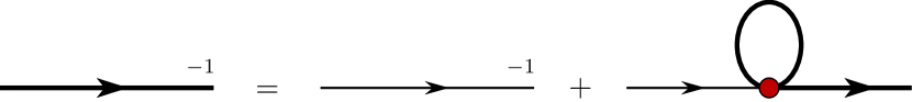
Figure 1: (Colour online) The NJL gap equation in the Hartree-Fock approximation, where the thin line represents the elementary quark propagator, $S_{0}^{-1}(k)=\not{k}-m+i\varepsilon$, and the shaded circle the $\bar{q}q$ interaction kernel given in Eq. (2). Higher order terms, attributed to meson loops, for example, are not included in the gap equation kernel.

The NJL model is a non-renormalizable quantum field theory, therefore a regularization prescription must be specified to fully define the model. We choose the proper-time regularization scheme Ebert:1996vx ; Hellstern:1997nv ; Bentz:2001vc , which is introduced formally via the relation

$$\frac{1}{X^{n}} =\frac{1}{(n-1)!}\int_{0}^{\infty}d\tau\,\tau^{n-1}\,e^{-\tau\,X},$$

$$\hskip 42.67912pt\longrightarrow\frac{1}{(n-1)!}\int_{1/\Lambda^{2}_{UV}}^{1/\Lambda^{2}_{IR}}d\tau\,\tau^{n-1}\,e^{-\tau\,X},$$ (6)

where $X$ represents a product of propagators that have been combined using Feynman parametrization. Only the ultraviolet cutoff, $\Lambda_{UV}$, is needed to render the theory finite, however, for bound states of quarks we also include the infrared cutoff, $\Lambda_{IR}$. This has the effect of eliminating unphysical thresholds for the decay of hadrons into free quarks and therefore simulates aspects of quark confinement in QCD.

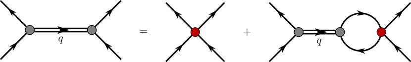
Figure 2: (Colour online) NJL Bethe-Salpeter equation for the quark–antiquark $t$-matrix, represented as the double line with the vertices. The single line corresponds to the dressed quark propagator and the BSE $\bar{q}q$ interaction kernel, consistent with the gap equation kernel used in Eq. (5), is given by Eq. (2).

Mesons in the NJL model are quark–antiquark bound states whose properties are determined by first solving the Bethe-Salpeter equation (BSE). The kernels of the gap and BSEs are intimately related, as exemplified by the vector and axialvector Ward–Takahashi identities, which relate the quark propagator to inhomogeneous Bethe-Salpeter vertices Maris:2003vk . The NJL BSE, consistent with the gap equation of Fig. 1, is illustrated in Fig. 2 and reads

$$\mathcal{T}(q)=\mathcal{K}+\int\frac{d^{4}k}{(2\pi)^{4}}\,\mathcal{K}\,S(k+q)\,S(k)\,\mathcal{T}(q),$$ (7)

where $q$ is the total momentum of the two-body system, $\mathcal{T}$ is the two-body $t$-matrix and $\mathcal{K}$ is the $\bar{q}q$ interaction kernel given in Eq. (2). Dirac, colour and isospin indices have been suppressed in Eq. (7). Solutions to the BSE in the $\bar{q}q$ channels with quantum numbers that correspond to those of the pion, rho and omega have the form

$$\mathcal{T}_{\pi}(q)_{\alpha\beta,\gamma\delta} =\left(\gamma_{5}\tau_{i}\right)_{\alpha\beta}\hskip 4.2679pt\,\tau_{\pi}(q)\hskip 8.53581pt\left(\gamma_{5}\tau_{i}\right)_{\gamma\delta},$$ (8)

$$\mathcal{T}_{\rho}(q)_{\alpha\beta,\gamma\delta} =\left(\gamma_{\mu}\tau_{i}\right)_{\alpha\beta}\ \,\tau^{\mu\nu}_{\rho}(q)\ \left(\gamma_{\nu}\tau_{i}\right)_{\gamma\delta},$$ (9)

$$\mathcal{T}_{\omega}(q)_{\alpha\beta,\gamma\delta} =\left(\gamma_{\mu}\right)_{\alpha\beta}\hskip 11.38109pt\,\tau^{\mu\nu}_{\omega}(q)\,\,\left(\gamma_{\nu}\right)_{\gamma\delta},$$ (10)

where $\tau_{i}$ are the Pauli matrices and

$$\tau_{\pi}(q) =\frac{-2i\,G_{\pi}}{1+2\,G_{\pi}\,\Pi_{PP}(q^{2})},$$ (11)

$$\tau^{\mu\nu}_{\rho}(q) =\frac{-2i\,G_{\rho}}{1+2\,G_{\rho}\,\Pi_{VV}(q^{2})}\left[g^{\mu\nu}+2\,G_{\rho}\,\Pi_{VV}(q^{2})\,\frac{q^{\mu}q^{\nu}}{q^{2}}\right],$$ (12)

$$\tau^{\mu\nu}_{\omega}(q) =\frac{-2i\,G_{\omega}}{1+2\,G_{\omega}\,\Pi_{VV}(q^{2})}\left[g^{\mu\nu}+2\,G_{\omega}\,\Pi_{VV}(q^{2})\,\frac{q^{\mu}q^{\nu}}{q^{2}}\right].$$ (13)

The functions $\tau_{\pi}(q)$, $\tau^{\mu\nu}_{\rho}(q)$ and $\tau^{\mu\nu}_{\omega}(q)$ are the reduced $t$-matrices, which are interpreted as propagators for the pion, rho and omega mesons. The bubble diagrams in Eqs. (11)–(13) have the form

$$\Pi_{PP}\left(q^{2}\right)\delta_{ij}=3i\int\frac{d^{4}k}{(2\pi)^{4}}\ \mathrm{Tr}\left[\gamma_{5}\,\tau_{i}\,S(k)\,\gamma_{5}\,\tau_{j}\,S(k+q)\right],$$ (14)

$$\Pi_{VV}(q^{2})\left(g^{\mu\nu}-\frac{q^{\mu}q^{\nu}}{q^{2}}\right)\delta_{ij}$$

$$\hskip 31.29802pt=3i\int\frac{d^{4}k}{(2\pi)^{4}}\ \mathrm{Tr}\left[\gamma^{\mu}\tau_{i}\,S(k)\,\gamma^{\nu}\tau_{j}\,S(k+q)\right],$$ (15)

where the traces are over Dirac and isospin indices. Meson masses are then defined by the pole in the corresponding two-body $t$-matrix.

In a covariant formulation a two-body $t$-matrix, near a bound state pole of mass $m_{i}$, behaves as

$$\mathcal{T}(q)\to\frac{\Gamma_{i}(q)\,\overline{\Gamma}_{i}(q)}{q^{2}-m_{i}^{2}},$$ (16)

where $\Gamma_{i}(q)$ is the normalized homogeneous Bethe-Salpeter vertex function for the bound state. Expanding the $t$-matrices in Eqs. (8)–(10) about the pole masses gives

$$\Gamma^{i}_{\pi} =\sqrt{Z_{\pi}}\,\gamma_{5}\,\tau_{i},\leavevmode\nobreak\ \leavevmode\nobreak\ \Gamma^{\mu,i}_{\rho}=\sqrt{Z_{\rho}}\,\gamma^{\mu}\,\tau_{i},\leavevmode\nobreak\ \leavevmode\nobreak\ \Gamma^{\mu}_{\omega}=\sqrt{Z_{\omega}}\,\gamma^{\mu},$$ (17)

where $i$ is an isospin index and the normalization factors are given by

$$Z_{\pi}^{-1} =-\frac{\partial}{\partial q^{2}}\,\Pi_{PP}(q^{2})\Big{\rvert}_{q^{2}=m_{\pi}^{2}},$$ (18)

$$Z_{\rho,\omega}^{-1} =-\frac{\partial}{\partial q^{2}}\,\Pi_{VV}(q^{2})\Big{\rvert}_{q^{2}=m_{\rho,\omega}^{2}}.$$ (19)

These residues are interpreted as the effective meson-quark-quark coupling constants. Homogeneous Bethe-Salpeter vertex functions are an essential ingredient in, for example, triangle diagrams that determine the meson form factors.

Baryons in the NJL model are naturally described as bound states of three dressed quarks. The properties of these bound states are determined by the relativistic Faddeev equation whose solution gives the Poincaré covariant Faddeev amplitude. To construct the interaction kernel of the Faddeev equation we require the elementary quark-quark interaction kernel. Using Fierz transformations to rewrite Eq. (1) as a sum of $qq$ interactions, keeping only the isoscalar–scalar ($0^{+},T=0$) and isovector–axialvector ($1^{+},T=1$) two-body channels, the NJL interaction Lagrangian takes the form

$$\mathcal{L}_{I,qq}=G_{s}\Bigl{[}\bar{\psi}\,\gamma_{5}\,C\,\tau_{2}\,\beta_{A}\,\bar{\psi}^{T}\Bigr{]}\Bigl{[}\psi^{T}\,C^{-1}\gamma_{5}\,\tau_{2}\,\beta_{A}\,\psi\Bigr{]}\\ +G_{a}\Bigl{[}\bar{\psi}\,\gamma_{\mu}\,C\,\tau_{i}\tau_{2}\,\beta_{A}\,\bar{\psi}^{T}\Bigr{]}\Bigl{[}\psi^{T}\,C^{-1}\gamma^{\mu}\,\tau_{2}\tau_{i}\,\beta_{A}\,\psi\Bigr{]},$$ (20)

where $C=i\gamma_{2}\gamma_{0}$ is the charge conjugation matrix and the couplings $G_{s}$ and $G_{a}$ give the strength of the scalar and axialvector $qq$ interactions. Because only colour $\bar{3}$ $qq$ states can couple to a third quark to form a colourless three-quark state, we must have $\beta_{A}=\sqrt{\tfrac{3}{2}}\,\lambda_{A}\leavevmode\nobreak\ (A=2,5,7)$ Ishii:1995bu . The Lagrangian of Eq. (20) gives the following elementary $qq$ interaction kernel

$$\mathcal{K}_{\alpha\beta,\gamma\delta} =4i\,G_{s}\left(\gamma_{5}\,C\,\tau_{2}\,\beta_{A}\right)_{\alpha\beta}\left(C^{-1}\,\gamma_{5}\,\tau_{2}\,\beta_{A}\right)_{\gamma\delta}$$

$$+4i\,G_{a}\left(\gamma_{\mu}\,C\,\tau_{i}\tau_{2}\,\beta_{A}\right)_{\alpha\beta}\left(C^{-1}\,\gamma^{\mu}\,\tau_{2}\tau_{i}\,\beta_{A}\right)_{\gamma\delta}.$$ (21)

This kernel has been truncated to support only scalar and axialvector diquark correlations because the pseudoscalar and vector diquark components of the nucleon must predominantly be in $\ell=1$ states and are therefore suppressed. Pseudoscalar and vector diquarks are also usually found to be considerably heavier than their scalar and axialvector counterparts Roberts:2011cf .

Using Eq. (21) as the interaction kernel in the Faddeev equation allows us to first sum all two-body $qq$ interactions to form the scalar and axialvector diquark $t$-matrices. Diquark correlations in the nucleon are therefore a natural consequence of the strong coupling in the colour $\bar{3}$ quark-quark interaction channel. The BSE in the $qq$ channel for our NJL model reads

$$\mathcal{T}(q)=\mathcal{K}+\frac{1}{2}\int\frac{d^{4}k}{(2\pi)^{4}}\,\mathcal{K}\,S(k+q)\,S(-k)\,\mathcal{T}(q),$$ (22)

where $\mathcal{K}$ is given in Eq. (21) and there is a symmetry factor of $\tfrac{1}{2}$ relative to the $\bar{q}q$ BSE of Eq. (7). The solutions to the BSE in the scalar and axialvector diquark channels are

$$\mathcal{T}_{s}(q)_{\alpha\beta,\gamma\delta} =\left(\gamma_{5}\,C\,\tau_{2}\,\beta_{A}\right)_{\alpha\beta}\tau_{s}(q)\left(C^{-1}\gamma_{5}\,\tau_{2}\,\beta_{A}\right)_{\gamma\delta},$$ (23)

$$\mathcal{T}_{a}(q)_{\alpha\beta,\gamma\delta} =\left(\gamma_{\mu}\,C\,\tau_{i}\tau_{2}\,\beta_{A}\right)_{\alpha\beta}\tau^{\mu\nu}_{a}(q)\left(C^{-1}\gamma_{\nu}\,\tau_{2}\tau_{i}\,\beta_{A}\right)_{\gamma\delta},$$ (24)

where

$$\tau_{s}(q) =\frac{-4i\,G_{s}}{1+2\,G_{s}\,\Pi_{PP}(q^{2})},$$ (25)

$$\tau^{\mu\nu}_{a}(q) =\frac{-4i\,G_{a}}{1+2\,G_{a}\,\Pi_{VV}(q^{2})}\left[g^{\mu\nu}+2\,G_{a}\,\Pi_{VV}(q^{2})\,\frac{q^{\mu}q^{\nu}}{q^{2}}\right].$$ (26)

The scalar and axialvector diquark masses are defined as the poles in Eqs. (25) and (26), respectively, and the homogeneous Bethe-Salpeter vertices read

$$\Gamma_{s} =\sqrt{Z_{s}}\,\gamma_{5}\,C\,\tau_{2}\,\beta_{A},\leavevmode\nobreak\ \Gamma^{\mu,i}_{a} =\sqrt{Z_{a}}\,\gamma^{\mu}\,C\,\tau_{i}\,\tau_{2}\,\beta_{A},$$ (27)

where $i$ is an isospin index. The pole residues are given by

$$Z_{s}^{-1} =-\frac{1}{2}\,\frac{\partial}{\partial q^{2}}\,\Pi_{PP}(q^{2})\Big{\rvert}_{q^{2}=M_{s}^{2}},$$ (28)

$$Z_{a}^{-1} =-\frac{1}{2}\,\frac{\partial}{\partial q^{2}}\,\Pi_{VV}(q^{2})\Big{\rvert}_{q^{2}=M_{a}^{2}},$$ (29)

where $M_{s}$ and $M_{a}$ are the scalar and axialvector diquark masses. These pole residues are interpreted as the effective diquark–quark-quark couplings.

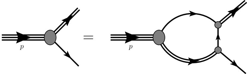
Figure 3: Homogeneous Faddeev equation for the nucleon in the NJL model. The single line represents the quark propagator and the double line the diquark propagators. Both scalar and axialvector diquarks are included in these calculations.

The homogeneous Faddeev equation is illustrated in Fig. 3, where diquark correlations have been made explicit. The relativistic Faddeev equation in the NJL model has been solved numerically in Refs. Buck:1992wz ; Mineo:1999eq ; Mineo:2002bg , where the integrals were regularized using the Lepage–Brodsky and transverse momentum cutoff schemes. In the proper-time regularization scheme used here, solving the Faddeev equation is much more challenging and we therefore employ the static approximation to the quark exchange kernel. In this approximation the propagator of the exchanged quark becomes $S(k)\to-\tfrac{1}{M}$ Buck:1992wz . The nucleon vertex function then takes the form

$$\Gamma_{N}(p)=\sqrt{-Z_{N}}\ \Gamma=\sqrt{-Z_{N}}\ \begin{bmatrix}\Gamma_{s}(p)\\ \Gamma_{a}^{\mu,i}(p)\end{bmatrix}$$

$$=\sqrt{-Z_{N}}\begin{bmatrix}\alpha_{1}\\ \left(\alpha_{2}\,\frac{p^{\mu}}{M_{N}}\,\gamma_{5}\ +\alpha_{3}\,\gamma^{\mu}\gamma_{5}\right)\frac{\tau_{i}}{\sqrt{3}}\end{bmatrix}\chi(t)\,u(p),$$ (30)

where $i$ is an isospin index and $\chi_{N}(t)$ is the nucleon isospinor:

$$\chi\!\left(\tfrac{1}{2}\right) =\begin{pmatrix}1\\ 0\end{pmatrix}, \chi\!\left(-\tfrac{1}{2}\right) =\begin{pmatrix}0\\ 1\end{pmatrix}.$$ (31)

The first element in the column vector of Eq. (30) represents the piece of the nucleon vertex function consisting of a quark and scalar diquark, while the second element represents the quark and axialvector diquark component. The nucleon mass is labelled by $M_{N}$ and the Dirac spinor is normalized such that $\bar{u}_{N}\,u_{N}=1$. $Z_{N}$ is the nucleon vertex function normalization and $\alpha_{1},\leavevmode\nobreak\ \alpha_{2},\leavevmode\nobreak\ \alpha_{3}$ are obtained by solving the Faddeev equation. After projection onto positive parity, spin one-half and isospin one-half, the homogeneous Faddeev equation is given by Ishii:1995bu

$$\Gamma_{N}(p,s)=K(p)\,\Gamma_{N}(p,s),$$ (32)

which in matrix form reads

$$\begin{bmatrix}\Gamma_{s}\\ \Gamma_{a}^{\mu}\end{bmatrix}=\frac{3}{M}\begin{bmatrix}\Pi_{Ns}&\sqrt{3}\gamma_{\alpha}\gamma_{5}\,\Pi^{\alpha\beta}_{Na}\\ \sqrt{3}\gamma_{5}\gamma^{\mu}\,\Pi_{Ns}&-\gamma_{\alpha}\gamma^{\mu}\,\Pi^{\alpha\beta}_{Na}\end{bmatrix}\begin{bmatrix}\Gamma_{s}\\ \Gamma_{a,\beta}\end{bmatrix}.$$ (33)

The quark-diquark bubble diagrams are defined as

$$\Pi_{Ns}(p) =\int\frac{d^{4}k}{(2\pi)^{4}}\,\tau_{s}(p-k)\,S(k),$$ (34)

$$\Pi^{\mu\nu}_{Na}(p) =\int\frac{d^{4}k}{(2\pi)^{4}}\,\tau^{\mu\nu}_{a}(p-k)\,S(k).$$ (35)

The vertex normalization of Eq. (30) is given by

$$Z_{N}=\left[\overline{\Gamma}\,\frac{\partial\,\Pi_{N}(p)}{\partial p^{2}}\,\Gamma\right]_{p^{2}=M_{N}^{2}}^{-1},$$ (36)

where

$$\Pi_{N}(p)=\begin{bmatrix}\Pi_{Ns}(p)&0\\ 0&\Pi^{\alpha\beta}_{Na}(p)\end{bmatrix}.$$ (37)

Regulating expressions such as those in Eqs. (34) and (35) using the proper-time scheme is tedious. Therefore, to render the Faddeev equation and form factor calculations tractable we make the pole approximation to the meson and diquark $t$-matrices, for example, Eqs. (25) and (26) become

$$\tau_{s}(q) \to-\frac{i\,Z_{s}}{q^{2}-M_{s}^{2}+i\,\varepsilon},$$ (38)

$$\tau^{\mu\nu}_{a}(q) \to-\frac{i\,Z_{a}}{q^{2}-M_{a}^{2}+i\,\varepsilon}\left(g^{\mu\nu}-\frac{q^{\mu}q^{\nu}}{M_{a}^{2}}\right).$$ (39)

Similar expressions are obtained in the meson sector.

In summary, the model parameters consist of the two regularization scales $\Lambda_{IR}$ and $\Lambda_{UV}$, the dressed quark mass $M$, and the Lagrangian coupling constants $G_{\pi}$, $G_{\rho}$, $G_{\omega}$, $G_{s}$, $G_{a}$. The infrared regularization scale is associated with confinement and therefore should be of the order $\Lambda_{\text{QCD}}$, and we choose $\Lambda_{IR}=0.240\,$GeV and for the constituent quark mass take $M=0.4\,$GeV. The physical pion mass ($m_{\pi}=140\,$MeV) and decay constant ($f_{\pi}=92\,$MeV) determine $\Lambda_{UV}$ and $G_{\pi}$. The physical masses of the rho ($m_{\rho}=770\,$MeV) and omega ($m_{\omega}=782\,$MeV) mesons constrain $G_{\rho}$ and $G_{\omega}$, respectively, while the physical nucleon ($M_{N}=940\,$MeV) and $\Delta$ ($M_{\Delta}=1232\,$MeV) baryon masses determine $G_{s}$ and $G_{a}$. Numerical values are given in Tab. 1.

Using the parameters given in Tab. 1, we obtain the following results for the residues of the two-body $t$-matrices: $Z_{\pi}=17.9$, $Z_{\rho}=6.96$, $Z_{\omega}=6.63$, $Z_{s}=11.1$ and $Z_{a}=6.73$. For the nucleon vertex function of Eq. (30) we find $Z_{N}=28.1$ and $(\alpha_{1},\,\alpha_{2},\,\alpha_{3})=(0.55,\,0.05,\,-0.40)$, where the scalar and axialvector diquark masses are $M_{s}=0.768\,$GeV and $M_{a}=0.903\,$GeV.

$\Lambda_{IR}$	$\Lambda_{UV}$	$M$	$G_{\pi}$	$G_{\rho}$	$G_{\omega}$	$G_{s}$	$G_{a}$
0.240	0.645	0.4	19.0	11.0	10.4	5.8	4.9

Table 1: Model parameters constrained to reproduce the physical pion, rho and omega masses; the pion decay constant; and the nucleon and delta baryon masses. The infrared regulator and the dressed quark mass are assigned their values a priori. The regularization parameters and dressed quark mass are in units of GeV, while the couplings are in units of GeV ^-2.

III Nucleon Electromagnetic Current

The electromagnetic current of an on-shell nucleon, expressed in terms of the Dirac and Pauli form factors, has the form

$$j^{\mu}_{\lambda^{\prime}\,\lambda}(p^{\prime},p)=\left<p^{\prime},\,\lambda^{\prime}\left|J^{\mu}_{\text{em}}\right|p,\,\lambda\right>$$

$$=u(p^{\prime},\,\lambda^{\prime})\left[\gamma^{\mu}\,F_{1}(Q^{2})+\frac{i\sigma^{\mu\nu}q_{\nu}}{2\,M_{N}}\,F_{2}(Q^{2})\right]u(p,\,\lambda),$$ (40)

where $q=p^{\prime}-p$ is the 4-momentum transfer, $Q^{2}\equiv-q^{2}$ and $\lambda$, $\lambda^{\prime}$ represent the initial and final nucleon helicity respectively. The nucleon’s electric and magnetic Sachs form factors Ernst:1960zza , which diagonalize the Rosenbluth cross-section, are then given by

$$G_{E}(Q^{2}) =F_{1}(Q^{2})-\frac{Q^{2}}{4\,M_{N}^{2}}\,F_{2}(Q^{2}),$$ (41)

$$G_{M}(Q^{2}) =F_{1}(Q^{2})+F_{2}(Q^{2}).$$ (42)

Hadron form factors can be decomposed into a sum over the quark charges multiplied by quark sector form factors, such that

$$F_{h}(Q^{2})=\sideset{}{{}_{q}}{\sum}\,e_{q}\,F_{h}^{q}(Q^{2}).$$ (43)

The quark sector form factors $F^{q}_{h}(Q^{2})$ represent the contribution of the current quarks of flavour $q$ to the total hadron form factor $F_{h}(Q^{2})$. The proton and neutron form factors expressed in terms of quark sector form factors read

$$F_{ip}(Q^{2}) =e_{u}\,F^{u}_{ip}(Q^{2})+e_{d}\,F^{d}_{ip}(Q^{2})+\ldots$$ (44)

$$F_{in}(Q^{2}) =e_{u}\,F^{u}_{in}(Q^{2})+e_{d}\,F^{d}_{in}(Q^{2})+\ldots$$ (45)

where $i=1,\,2$. Note that in light of the experimental discovery that the strange quarks contribute very little to the nucleon electromagnetic form factors  Young:2006jc ; Aniol:2005zf ; Armstrong:2005hs ; Baunack:2009gy , we will neglect their contribution to Eqs. (44) and (45). Assuming equal $u$ and $d$ current quark masses and neglecting electroweak corrections, the $u$ and $d$ quark sector form factors of the nucleon must satisfy the charge symmetry constraints:

$$F^{d}_{in}(Q^{2})=F^{u}_{ip}(Q^{2})\quad\text{and}\quad F^{u}_{in}(Q^{2})=F^{d}_{ip}(Q^{2}).$$ (46)

Experimentally, if electroweak and heavy quark effects are small, the $u$ and $d$ quark sector form factors are given accurately by

$$F^{u}_{ip} =2\,F_{ip}+F_{in}, F^{d}_{ip} =F_{ip}+2\,F_{in}.$$ (47)

Recent accurate data for the neutron form factors has enabled a precise determination of the quark sector proton form factors Cates:2011pz . We will discuss results for these quark sector form factors in Sect. VI.

The slope of an electromagnetic form factor at $Q^{2}=0$ is a measure of either the squared rms charge or magnetic radius of a hadron. Unless stated otherwise all squared rms radii are defined by

$$\left<r^{2}\right>=-\frac{6}{\eta}\ \frac{\partial\,f(Q^{2})}{\partial Q^{2}}\bigg{\lvert}_{Q^{2}=0}\leavevmode\nobreak\ \leavevmode\nobreak\ \Big{|}\leavevmode\nobreak\ \leavevmode\nobreak\ \eta=\begin{cases}1&\text{if\leavevmode\nobreak\ }f(0)=0,\\[1.72218pt] f(0)&\text{if\leavevmode\nobreak\ }f(0)\neq 0,\end{cases}$$ (48)

where $f(Q^{2})$ is an arbitrary form factor. This definition reproduces the standard nucleon results for the charge and magnetic radii defined by the Sachs form factors:

$$\left<r_{E}^{2}\right> =-6\ \ \frac{\partial\,G_{E}(Q^{2})}{\partial Q^{2}}\Big{\lvert}_{Q^{2}=0},$$ (49)

$$\left<r_{M}^{2}\right> =-\frac{6}{G_{M}(0)}\ \frac{\partial\,G_{M}(Q^{2})}{\partial Q^{2}}\Big{\lvert}_{Q^{2}=0},$$ (50)

but also generalizes to radii defined with respect to the Dirac and Pauli form factors and quark sector form factors. Hadronic radii, in units of fm, will be obtained from the result of Eq. (48) using

$$r\equiv\text{sign}\left(\left<r^{2}\right>\right)\ \sqrt{\left|\left<r^{2}\right>\right|}.$$ (51)

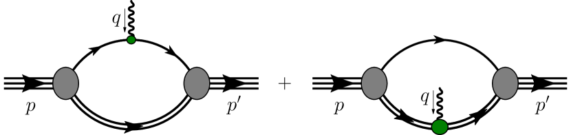
Figure 4: (Colour online) Feynman diagrams representing the nucleon electromagnetic current. The diagram on the left is called the quark diagram and the diagram on the right the diquark diagram. In the diquark diagram the photon interacts with each quark inside the non-pointlike diquark.

To calculate the nucleon electromagnetic current and therefore the Dirac and Pauli form factors, one must know the manner in which the nucleon described in Sect. II couples to the photon, guaranteeing electromagnetic gauge invariance. The necessary Feynman diagrams are illustrated in Fig. 4 and a proof of gauge invariance is given in App. B. We include both scalar and axialvector diquarks in our nucleon wave function and therefore the diagrams in Fig. 4 represent six distinct Feynman diagrams. The diagram on the left, referred to as the quark diagram, represents the processes where the photon couples to a dressed quark with either a scalar or axialvector diquark as a spectator. The diquark diagram, on the right in Fig. 4, represents four Feynman diagrams; the photon can couple to a scalar diquark, an axialvector diquark or cause a transition between these two diquark states. Importantly, in the diquark diagram the photon couples to the quarks inside each diquark, thereby resolving internal diquark structure and resulting in, for example, diquarks with a finite size. The coupling of a photon to a dressed quark and to the diquarks is discussed in Sects. IV and V.

IV Quark–Photon Vertex

The quark-photon vertex in the NJL model, and other field theoretic approaches, is given by the solution to an inhomogeneous BSE. The NJL model version of this equation, consistent with the truncation used in the gap and BSEs discussed Sect. II, is represented diagrammatically in Fig. 5. The large oval represents the quark-photon vertex, $\,\Lambda^{\mu}_{\gamma Q}(p^{\prime},p)$, the 4-fermion interaction kernel is given in Eq. (2) and the elementary vertex, which gives the inhomogeneous driving term, has the form $\gamma^{\mu}\,\hat{Q}$ (where $\hat{Q}$ is the quark charge operator). The second equality in Fig. 5 expresses this equation in an equivalent form using the $\bar{q}q$ $t$-matrices.

The quark charge operator is

$$\hat{Q} =\begin{pmatrix}e_{u}&0\\ 0&e_{d}\end{pmatrix}=\frac{1}{6}+\frac{\tau_{3}}{2},$$ (52)

where $e_{u}=\tfrac{2}{3}$ and $e_{d}=-\tfrac{1}{3}$ are the $u$ and $d$ quark charges. The quark-photon vertex therefore has both an isoscalar and isovector component, which may in general be expressed in the form

$$\Lambda^{\mu}_{\gamma Q}(p^{\prime},p) =\frac{1}{6}\,\Lambda^{\mu}_{\omega}(p^{\prime},p)+\frac{\tau_{3}}{2}\,\Lambda^{\mu}_{\rho}(p^{\prime},p).$$ (53)

The quark-photon vertex, separated into flavour sectors defined by the dressed quarks, reads

$$\Lambda^{\mu}_{\gamma Q}(p^{\prime},p)=\Lambda^{\mu}_{U}(p^{\prime},p)\ \frac{1+\tau_{3}}{2}+\Lambda^{\mu}_{D}(p^{\prime},p)\ \frac{1-\tau_{3}}{2}.$$ (54)

In general each dressed quark component of the quark-photon vertex contains contributions from both the $u$ and $d$ current quarks. This will prove important when we consider quark sector form factors and associated charge symmetry constraints. Note that throughout this manuscript we use a capital $Q=(U,\,D)$ to indicate that an object is associated with dressed quarks and a lowercase $q=(u,\,d)$ to represent the current quarks of the NJL and QCD Lagrangians.

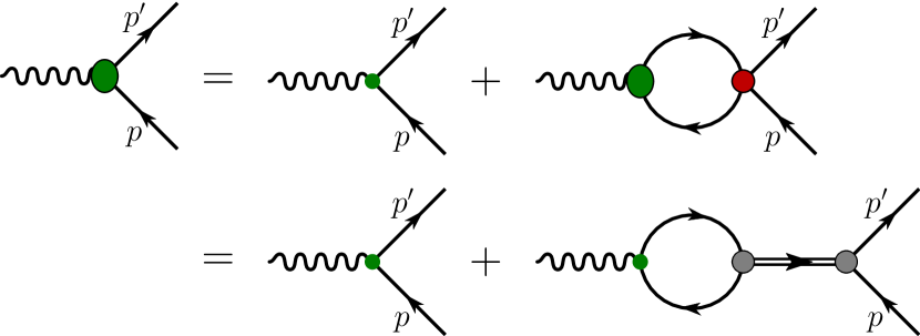
Figure 5: (Colour online) Inhomogeneous Bethe-Salpeter equation whose solution gives the quark-photon vertex, represented as the large shaded oval. The small dot is the inhomogeneous driving term, while the shaded circle is the $\bar{q}q$ interaction kernel given in Eq. (2). Only the $\rho$ and $\omega$ interaction channels contribute. This integral equation can equivalently be represented using the elementary quark-photon interaction and the $\rho$ and $\omega$ $t$-matrices, given in Eqs. (12) and (13). This case is depicted by the second equality.

The quark-photon vertex has in general 12 Lorentz structures Maris:1999bh , 4 longitudinal and 8 pieces transverse to the photon momentum, where each Lorentz structure is accompanied by a scalar function of the three variables $q^{2}$, $p^{\prime 2}$ and $p^{2}$. The standard NJL $\bar{q}q$ interaction kernel, as employed in Sect. II for the gap and BSE equations, is momentum independent which implies that the quark-photon vertex can only depend on the momentum transfer $q=p^{\prime}-p$, not $p^{\prime}$ and $p$ separately. Therefore, in this work, the contributions to the vertex functions of Eq. (53) from the NJL BSE, take the form

$$\Lambda^{(\text{bse})\mu}_{\omega}(q) =\gamma^{\mu}+\left(\!\gamma^{\mu}-\frac{q^{\mu}\not{q}}{q^{2}}\right)\!\hat{F}_{1\omega}(q^{2})+\frac{i\sigma^{\mu\nu}q_{\nu}}{2\,M}F_{2\omega}(q^{2}),$$ (55)

$$\Lambda^{(\text{bse})\mu}_{\rho}(q) =\gamma^{\mu}+\left(\!\gamma^{\mu}-\frac{q^{\mu}\not{q}}{q^{2}}\right)\!\hat{F}_{1\rho}(q^{2})+\frac{i\sigma^{\mu\nu}q_{\nu}}{2\,M}F_{2\rho}(q^{2}).$$ (56)

With the quark propagator of Eq. (4), these results satisfy the Ward–Takahashi identity:

$$q_{\mu}\,\Lambda^{\mu}_{\gamma Q}(p^{\prime},p) =\hat{Q}\left[S^{-1}(p^{\prime})-S^{-1}(p)\right],$$ (57)

demanded by $U(1)$ vector gauge invariance.

Current conservation at the hadron level implies that the $q^{\mu}\not{q}/q^{2}$ term in Eqs. (55) and (56) cannot contribute to hadron form factors. We therefore write our effective vertex as

$$\Lambda^{(\text{bse})\mu}_{i}(q) =\gamma^{\mu}\,F_{1i}(q^{2})+\frac{i\sigma^{\mu\nu}q_{\nu}}{2\,M}\,F_{2i}(q^{2}),$$ (58)

where $i=(\omega,\,\rho)$ and $F_{1i}(q^{2})=1+\hat{F}_{1i}(q^{2})$. This vertex has the same form as the electromagnetic current for an on-shell spin-half fermion. For a pointlike quark $F_{1\omega}(q^{2})=1=F_{1\rho}(q^{2})$ and $F_{2\omega}(q^{2})=0=F_{2\rho}(q^{2})$. However, interactions in the NJL model not only dynamically generate a dressed quark mass but also generate non-trivial dressed quark form factors.

The inhomogeneous BSE for the quark-photon vertex, depicted in Fig. 5, has the form

$$\Lambda^{\mu}_{\gamma Q}(p^{\prime},p)=\gamma^{\mu}\left(\frac{1}{6}+\frac{\tau_{3}}{2}\right)+\sideset{}{{}_{\Omega}}{\sum}\,K_{\Omega}\ \Omega$$

$$\hskip 17.07164pt\times\ i\!\int\frac{d^{4}k}{(2\pi)^{4}}\ \mathrm{Tr}\left[\bar{\Omega}\,S(k+q)\,\Lambda^{\mu}_{\gamma Q}(p^{\prime},p)\,S(k)\right],$$ (59)

where $\sum_{\Omega}\,K_{\Omega}\ \Omega_{\alpha\beta}\,\bar{\Omega}_{\lambda\varepsilon}$ represents the interaction kernel given in Eq. (2). The Dirac and isospin structure of $\Lambda^{\mu}_{\gamma Q}(p^{\prime},p)$, given in Eqs. (53), (55) and (56), implies that of the interaction channels in Eq. (2) only the isovector–vector, $-2i\,G_{\rho}\left(\gamma_{\mu}\vec{\tau}\right)_{\alpha\beta}\left(\gamma^{\mu}\vec{\tau}\right)_{\gamma\delta}$, and isoscalar–vector, $-2i\,G_{\omega}\left(\gamma_{\mu}\right)_{\alpha\beta}\left(\gamma^{\mu}\right)_{\gamma\delta}$, pieces can contribute.

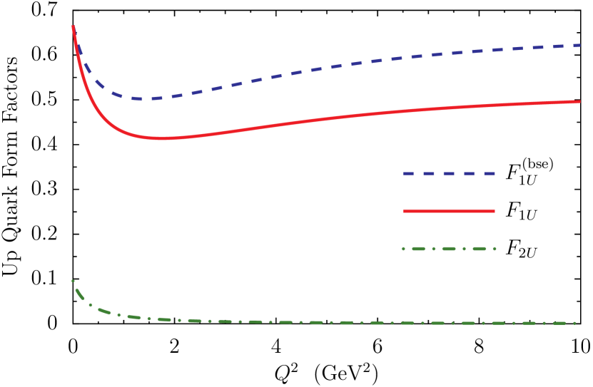
(a)

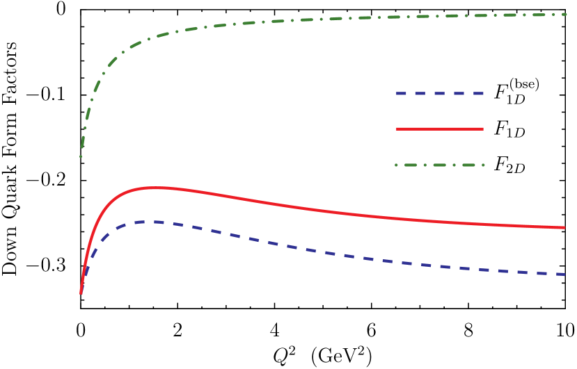
(b)

Figure 6: (Colour online) Upper panel: Dressed up quark form factors: the dashed line is the Dirac form factor obtained from the BSE of Eq. (59); the solid and dash-dotted lines are respectively the Dirac and Pauli form factors generated by also including the pion loop corrections illustrated in Fig. 8. Lower panel: Dressed down quark form factors: each curve represents an analogous form factor to those in the upper panel.

The dressed quark form factors obtained from the inhomogeneous BSE, associated with the electromagnetic current of Eq. (58), are

$$F_{1i}(q^{2})=\frac{1}{1+2\,G_{i}\,\Pi_{VV}(q^{2})},\hskip 34.1433ptF_{2i}(q^{2})=0,$$ (60)

where $i=\omega,\,\rho$. Comparison with Eqs. (12) and (13) indicate that $F_{1\omega}$ and $F_{1\rho}$ have a pole at $q^{2}=m_{\omega}^{2}$ and $m_{\rho}^{2}$, respectively. The NJL BSE kernel of Eq. (2) does not generate Pauli form factors for the dressed quarks because it does not include the tensor–tensor 4-fermion interaction. The dressed up and down quark form factors given by the BSE therefore read

$$F^{\text{(bse)}}_{1Q}(Q^{2}) =\frac{1}{6}\,F_{1\omega}(Q^{2})\pm\frac{1}{2}\,F_{1\rho}(Q^{2}),$$ (61)

where the plus sign is associated with a dressed up quark. The superscript (bse) indicates that these form factors are obtained solely from the BSE.

Results for the dressed quark BSE form factors are illustrated as the dashed lines in Figs. 6. A notable feature of these results is that they do not drop to zero as $Q^{2}\to\infty$, but instead behave as

$$F^{\text{(bse)}}_{1U}(Q^{2}) \stackrel{{\scriptstyle Q^{2}\to\infty}}{{=}}e_{u}, F^{\text{(bse)}}_{1D}(Q^{2}) \stackrel{{\scriptstyle Q^{2}\to\infty}}{{=}}e_{d},$$ (62)

signifying that at infinite $Q^{2}$ the photon interacts with a bare current quark. This result is consistent with QCD expectations based on asymptotic freedom.

Pion loop corrections to the quark-photon vertex will also be considered and treated as a perturbation to the dressed quark form factors obtained from the BSE, as given in Eqs. (60) and (61). In this case the dressed quark propagator receives an additional self-energy correction which is illustrated in Fig. 7. In addition to the pionic self-energies on the dressed quarks, pion exchange between quarks should also be included in the two-body kernels that enter the Bethe-Salpeter and Faddeev equations. However, it is straightforward to show that in the limit where the nucleon and $\Delta$ are mass degenerate, including only self-energy correction on the dressed quarks yields essentially the correct leading non-analytic behaviour of the electromagnetic form factors as a function of quark mass. Further, in form factor calculations diagrams with a photon coupling to an exchanged pion do not contribute because of the cancellation between $\pi^{+}$ and $\pi^{-}$ exchange. This self-energy is evaluated using a pole approximation, where the external quark is assumed on-mass-shell. The pion loop therefore shifts the dressed quark mass by a constant, giving a quark propagator of the form

$$\tilde{S}(k)=Z\,S(k),\qquad Z=1+\frac{\partial\,\Sigma(p)}{\partial\not{p}}\bigg{\rvert}_{\not{p}=M},$$ (63)

where $S(k)$ is the usual Feynman propagator for a dressed quark of mass $M$ and the self-energy reads

$$\Sigma(p)=-\int\frac{d^{4}k}{(2\pi)^{2}}\ \gamma_{5}\,\tau_{i}\,S(p-k)\,\gamma_{5}\,\tau_{i}\,\tau_{\pi}(k).$$ (64)

When evaluating $\Sigma(p)$ the reduced pion $t$-matrix is approximated by its pole form, that is

$$\tau_{\pi}(k)\to\frac{i\,Z_{\pi}}{k^{2}-m_{\pi}^{2}+i\varepsilon}.$$ (65)

The quark wave function renormalization factor, $Z$, represents the probability to strike a dressed quark without the pion cloud and is essential to maintain charge conservation. Using the parameters in Tab. 1 gives $Z=0.80$.

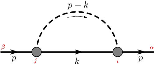
Figure 7: (Colour online) Pion loop contribution to the dressed quark self-energy. The pion couples to the dressed quark via $\gamma_{5}\,\tau_{i}$ and the pion $t$-matrix is approximated by its pole form.

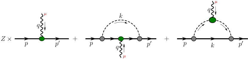
Figure 8: (Colour online) Pion loop contributions to the quark-photon vertex. The quark wave function renormalization factor $Z$ represents the probability of striking a dressed quark without a pion cloud. In the first two diagrams the photon couples to the dressed quark with a vertex of the general form given by Eq. (53); and defined by Eqs. (58) and (60). The shaded oval in the third diagram represents the quark–pion vertex, which we approximate by its pole form. It is therefore given by $\left(\ell^{\prime}+\ell\right)F_{\pi}(Q^{2})$, where $F_{\pi}(Q^{2})$ is the usual pion form factor (see Eq. (86) and associated discussion).

The quark electromagnetic current, including pion loops, is illustrated in Fig. 8. Evaluating this current between on-shell constituent quarks, gives for the dressed quark sector currents of Eq. (54):

$$\Lambda_{Q}^{\mu}(p^{\prime},p) =\gamma^{\mu}\,F_{1Q}(Q^{2})+\frac{i\sigma^{\mu\nu}q_{\nu}}{2\,M}\,F_{2Q}(Q^{2}),$$ (66)

where $Q=(U,\,D)$. The dressed quark form factors read

$$F_{1U}=Z\left[\tfrac{1}{6}\,F_{1\omega}+\tfrac{1}{2}\,F_{1\rho}\right]+\left[F_{1\omega}-F_{1\rho}\right]f_{1}^{(q)}+F_{1\rho}\,f_{1}^{(\pi)},$$ (67)

$$F_{1D}=Z\left[\tfrac{1}{6}\,F_{1\omega}-\tfrac{1}{2}\,F_{1\rho}\right]+\left[F_{1\omega}+F_{1\rho}\right]f_{1}^{(q)}-F_{1\rho}\,f_{1}^{(\pi)},$$ (68)

$$F_{2U}=\left[F_{1\omega}-F_{1\rho}\right]f_{2}^{(q)}+F_{1\rho}\,f_{2}^{(\pi)},$$ (69)

$$F_{2D}=\left[F_{1\omega}+F_{1\rho}\right]f_{2}^{(q)}-F_{1\rho}\,f_{2}^{(\pi)},$$ (70)

where the $Q^{2}$ dependence of each form factor has been omitted. The body form factors, $f_{1}^{(q)}$ and $f_{2}^{(q)}$, originate from the second diagram in Fig. 8, while $f_{1}^{(\pi)}$ and $f_{2}^{(\pi)}$ are the body form factors from the third diagram, which also contain the pion body form factor (see discussion associated with Eq. (86)). These body form factors are illustrated in Fig. 9. When evaluating the pion loop diagrams in Figs. 7 and 8 we use the proper-time regularization scheme, however, in this case the pions should not be confined and we therefore set $\Lambda_{IR}=0\,$GeV. This procedure guarantees that the leading-order non-analytic behaviour of the hadron form factors as a function of the pion mass is retained.

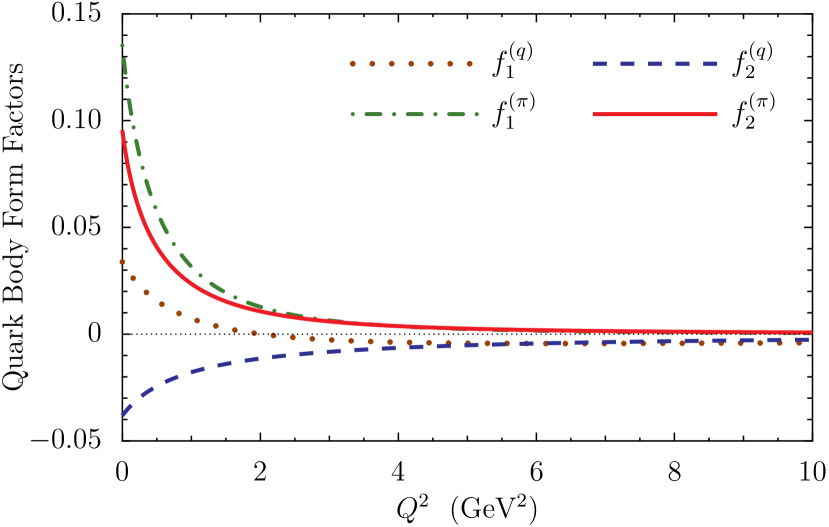
Figure 9: (Colour online) Dressed quark body form factors associated with the pion loop corrections, where $f_{1}^{(q)}$ and $f_{2}^{(q)}$ originate from the second diagram in Fig. 8 and $f_{1}^{(\pi)}$ and $f_{2}^{(\pi)}$ from the third diagram.

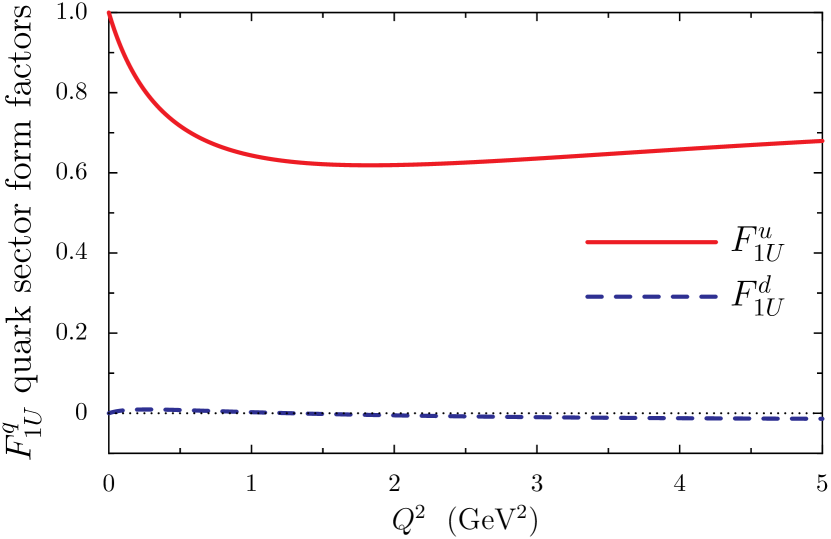
(a)

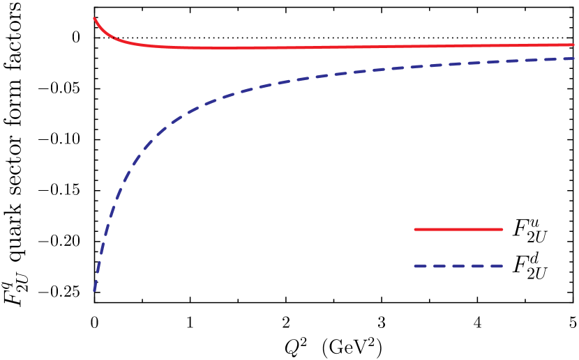
(b)

Figure 10: (Colour online) Upper panel: Dressed up quark Dirac form factors, that also include pion cloud effects, separated into quark sectors. The solid line is the $u$-quark sector of the dressed up quark and the dashed line represents $d$-quark sector. Lower panel: Dressed up quark Pauli form factors separated into quark sectors. The solid line is the $u$-quark sector and the dashed line the $d$-quark sector.

Results for the Dirac and Pauli dressed quark form factors, including pion loop effects, are given in Figs. 6. The pion cloud softens the Dirac form factors, however its most important consequence is the non-zero Pauli form factor for the dressed quarks. At infinite $Q^{2}$ the dressed quark Dirac form factors now become

$$F_{1U}(Q^{2}) \stackrel{{\scriptstyle Q^{2}\to\infty}}{{=}}Z\,e_{u}, F_{1D}(Q^{2}) \stackrel{{\scriptstyle Q^{2}\to\infty}}{{=}}Z\,e_{d},$$ (71)

whereas the Pauli form factors vanish for large $Q^{2}$. We find dressed quark anomalous magnetic moments of

$$\kappa_{U}=0.10\qquad\text{and}\qquad\kappa_{D}=-0.17,$$ (72)

defined as $\kappa_{Q}\equiv F_{2Q}(0)$. The quark charge and magnetic radii, defined with respect to the Sachs form factors and Eq. (48), take the values

$$r^{U}_{E} =0.59\,\text{fm}, r^{U}_{M} =0.60\,\text{fm},$$ (73)

$$r^{D}_{E} =0.73\,\text{fm}, r^{D}_{M} =0.67\,\text{fm}.$$ (74)

Decomposing the dressed quark form factors in quark/flavour sectors gives

$$F_{1U}(Q^{2}) =e_{u}\,F^{u}_{1U}(Q^{2})+e_{d}\,F_{1U}^{d}(Q^{2}),$$ (75)

$$F_{1D}(Q^{2}) =e_{u}\,F^{u}_{1D}(Q^{2})+e_{d}\,F_{1D}^{d}(Q^{2}),$$ (76)

where the flavour sector dressed up quark form factors read

$$F^{u}_{1U}=Z\,\tfrac{1}{2}\left[F_{1\omega}+F_{1\rho}\right]+\left[3\,F_{1\omega}-F_{1\rho}\right]f_{1}^{(q)}+F_{1\rho}\,f_{1}^{(\pi)},$$ (77)

$$F^{d}_{1U}=Z\,\tfrac{1}{2}\left[F_{1\omega}-F_{1\rho}\right]+\left[3\,F_{1\omega}+F_{1\rho}\right]f_{1}^{(q)}-F_{1\rho}\,f_{1}^{(\pi)},$$ (78)

$$F^{u}_{2U}=\left[3\,F_{1\omega}-F_{1\rho}\right]f_{2}^{(q)}+F_{1\rho}\,f_{2}^{(\pi)},$$ (79)

$$F^{d}_{2U}=\left[3\,F_{1\omega}+F_{1\rho}\right]f_{2}^{(q)}-F_{1\rho}\,f_{2}^{(\pi)}.$$ (80)

The flavour sector dressed down quark form factors are given by

$$F_{iD}^{u} =F_{iU}^{d}\qquad\text{and}\qquad F_{iD}^{d}=F_{iU}^{u}$$ (81)

where $i=(1,\,2)$. Therefore, these results satisfy charge symmetry and are illustrated in Figs. 10. For the quark sector anomalous magnetic moments we find

$$\kappa^{u}_{U}=0.02\qquad\text{and}\qquad\kappa^{d}_{U}=-0.25,$$ (82)

and therefore the $d$ current quarks carry the bulk of the dressed up quark anomalous magnetic moment. This will have important implications for the nucleon form factors.

V Diquark and Meson Form Factors

Critical to our picture of nucleon structure are diquark correlations inside the nucleon. An essential step therefore, in calculating the nucleon form factors, is to first determine the interaction of the virtual photon with the diquarks. A further reason to discuss the diquark form factors is that the scalar and axialvector diquarks are the $qq$ analogs of the $\pi$ and $\rho$ mesons.

The electromagnetic current of a diquark is represented by the Feynman diagrams illustrated in Fig. 11 and is expressed as

$$j^{\mu}(p^{\prime},p)=i\int\frac{d^{4}k}{(2\pi)^{4}}$$

$$\mathrm{Tr}\left[\overline{\Gamma}(p^{\prime})\,S(p^{\prime}+k)\,\Lambda^{\mu}_{\gamma Q}(p^{\prime},p)\,S(p+k)\,\Gamma(p)\,S^{T}(-k)\right],$$ (83)

where the superscript $T$ indicates transpose. The Bethe-Salpeter vertices are represented by $\Gamma(p)$ and are given in Eq. (27). The dressed quark-photon vertex $\Lambda^{\mu}_{\gamma Q}(p^{\prime},p)$ is given in Eqs. (54) and (66).

Hadron form factors will be determined using the three variants for the dressed quark form factors discussed in Sect. IV and illustrated, for the non-trivial variants, in Fig. 6. Results obtained by treating the dressed quarks as pointlike will be labelled with a superscript (bare), while those obtained using the dressed quark form factors from the BSE, Eq. (61), will be labelled with a superscript (bse) and our full results, where the quark form factors also include pion loop corrections, Eqs. (67)–(70), will have no superscript label.

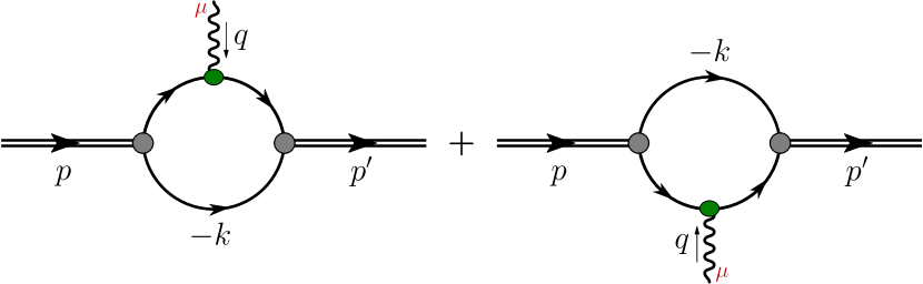
Figure 11: (Colour online) Feynman diagrams that represent the diquark electromagnetic current. The shaded circles are the diquark Bethe-Salpeter vertices and the shaded oval is the quark-photon vertex. The Feynman diagrams for the meson form factors are analogous. However the flow of baryon number on one of the quark lines must be reversed.

The electromagnetic current for a scalar diquark, or any on-shell spin-zero particle, has the general form

$$j_{s}^{\mu}(p^{\prime},p)=\left(p^{\prime}+p\right)^{\mu}\,F_{s}(Q^{2}),$$ (84)

and is therefore parameterized by a single form factor. Evaluating Eq. (83) for the scalar diquark gives

$$F_{s}(Q^{2})=\left[F_{1U}(Q^{2})+F_{1D}(Q^{2})\right]f_{s}^{V}(Q^{2})\\ +\left[F_{2U}(Q^{2})+F_{2D}(Q^{2})\right]f_{s}^{T}(Q^{2}),$$ (85)

where $f_{s}^{V}$, $f_{s}^{T}$ are the scalar diquark body form factors associated with the vector and tensor photon couplings to the dressed quarks (see Eq. (66)). Results for the scalar diquark form factor are given in Fig. 12 for the three variants of dressed quark form factors. Vertex corrections introduced by the BSE result in a softer form factor (dashed line) in comparison with results obtained using pointlike dressed quark form factors (dash-dotted line). Including pion loop corrections only slightly alters the scalar diquark form factor (solid line).

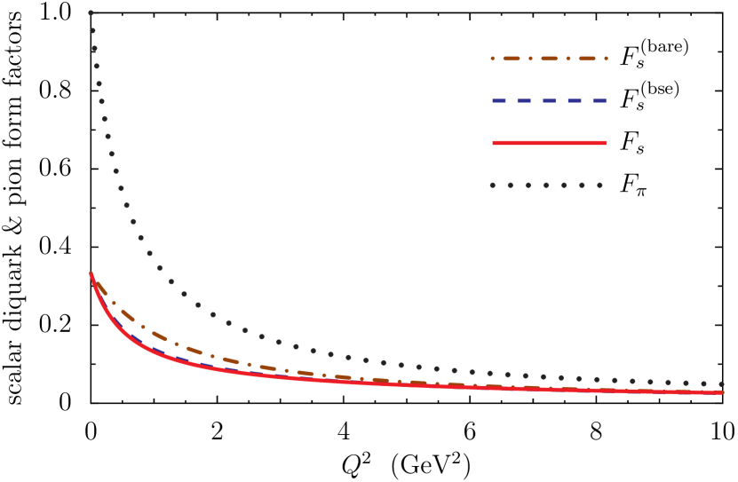
Figure 12: (Colour online) Results for the scalar diquark and pion form factors. For the pion we just show the full results, however for the scalar diquark form factors we show the cases when the dressed quarks are pointlike, the quark-photon vertex is given by the BSE and finally when pion loop corrections are also included.

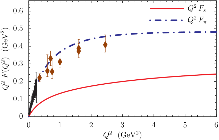
Figure 13: (Colour online) Scalar diquark and pion form factors multiplied by $Q^{2}$. The pion form factor data is from Refs. Amendolia:1986wj ; Amendolia:1984nz ; Horn:2006tm ; Tadevosyan:2007yd ; Blok:2008jy .

The $\bar{q}q$ analog of the scalar diquark is the pion, where for the $\pi^{+}$ the electromagnetic form factor is given by

$$F_{\pi}(Q^{2})=\left[F_{1U}(Q^{2})-F_{1D}(Q^{2})\right]f_{s}^{V}(Q^{2})\\ +\left[F_{2U}(Q^{2})-F_{2D}(Q^{2})\right]f_{s}^{T}(Q^{2}).$$ (86)

The body form factors in Eq. (86) are the same as those for the scalar diquark, except they are now functions of the pion mass instead of the scalar diquark mass. We do not include pion loop corrections on the dressed quarks in the case of the pion form factor, because at the hadronic level there is no three pion vertex. The full result for the pion form factor is given as the dotted curve in Fig. 12. The scalar diquark and pion form factors multiplied by $Q^{2}$ are presented in Fig. 13, where good agreement with pion form factor data from Refs. Amendolia:1986wj ; Amendolia:1984nz ; Horn:2006tm ; Tadevosyan:2007yd ; Blok:2008jy is seen. At large $Q^{2}$ both form factors plateau, where we find $Q^{2}\,F_{\pi}(Q^{2})\to 0.48$ and $Q^{2}\,F_{s}(Q^{2})\to 0.30$. The pion form factor result is consistent with the perturbative QCD prediction Lepage:1979zb ; Farrar:1979aw :

$$Q^{2}\,F_{\pi}(Q^{2})\stackrel{{\scriptstyle Q^{2}\to\infty}}{{\longrightarrow}}16\,\pi\,f_{\pi}^{2}\,\alpha_{s}(Q^{2}),$$ (87)

in the sense that the strong coupling constant, $\alpha_{s}(Q^{2})$, corresponds to a constant in the NJL model and therefore $Q^{2}\,F_{\pi}(Q^{2})$ should become constant as $Q^{2}\to\infty$. Taking Eq. (87) literally, our pion form factor result implies that $\alpha_{s}(Q^{2})=1.12$, which using a NNLO result for the running coupling Gluck:1998xa would correspond to an NJL model scale of $Q_{0}^{2}\sim 0.18\,$GeV², which is consistent with previous estimates Cloet:2005rt ; Cloet:2005pp ; Cloet:2006bq . Our calculated pion form factor reaches its plateau by $Q^{2}\simeq 6\,$GeV², which corresponds to the same scale at which the Dyson-Schwinger equation results of Ref. Chang:2013nia reach a maximum, after which the result of Ref. Chang:2013nia decreases because of the logarithmic running of $\alpha_{s}(Q^{2})$ in QCD.

	$r^{\text{(bare)}}_{E}$	$r^{\text{(bse)}}_{E}$	$r_{E}$	$r^{\text{exp}}_{E}$
scalar diquark	0.46	0.62	0.63
pion	0.46	0.62	0.62	0.663 $\pm$ 0.006

Table 2: Charge radii for the scalar diquark and pion, each shown for the three variants for the dressed quark form factors. The experimental value for the pion is from Ref. Dally:1982zk ; Amendolia:1986wj . All radii are in units of fm.

Results for the scalar diquark and pion charge radii are given in Tab. 2, for the three variants of the dressed quark form factors. The charge radius of the pion and scalar diquark are found to be very similar, where the pion radius is approximately 5% smaller than the experimental value from Refs. Dally:1982zk ; Amendolia:1986wj .

The electromagnetic current for an axialvector diquark, or any on-shell spin-one particle, has the general form Frankfurt:1977vc

$$j_{a}^{\mu,\alpha\beta}(p^{\prime},p) =\left[g^{\alpha\beta}F_{1a}(Q^{2})-\frac{q^{\alpha}q^{\beta}}{2\,M_{a}^{2}}\,F_{2a}(Q^{2})\right]\left(p^{\prime}+p\right)^{\mu}$$

$$\hskip 39.83385pt-\left(q^{\alpha}g^{\mu\beta}-q^{\beta}g^{\mu\alpha}\right)F_{3a}(Q^{2}),$$ (88)

where the Lorentz indices $\mu$, $\alpha$, $\beta$ represent the polarizations of the photon, initial axialvector diquark and final axialvector diquark, respectively. The Lorentz covariant form factors of Eq. (88) are often re-expressed as the Sachs-like charge, magnetic and quadruple form factors for a spin-one particle, given by

$$G_{C}(Q^{2}) =F_{1}(Q^{2})+\frac{2}{3}\,\eta\,G_{Q}(Q^{2}),$$ (89)

$$G_{M}(Q^{2}) =F_{3}(Q^{2}),$$ (90)

$$G_{Q}(Q^{2}) =F_{1}(Q^{2})+\left(1+\eta\right)F_{2}(Q^{2})-F_{3}(Q^{2}),$$ (91)

where $\eta=\frac{Q^{2}}{4\,m_{H}^{2}}$ and $m_{H}$ is the relevant hadron mass. At $Q^{2}=0$ these form factors give, respectively, the charge, magnetic moment and quadruple moment of a spin-one particle, in units of $e$, $e/(2\,m_{H})$ and $e/m_{H}^{2}$. The charge, magnetic and quadrupole radii – $\left<r_{C}^{2}\right>$, $\left<r_{M}^{2}\right>$, $\left<r_{Q}^{2}\right>$ – are defined with respect to these Sachs-like form factors.

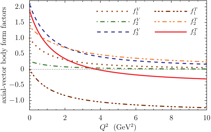
Figure 14: (Colour online) Axial–vector diquark body form factors. These body form factors must still be multiplied by the appropriate dressed quark form factors to obtain the axialvector diquark form factors.

Evaluating the Feynman diagrams of Fig. 11, using the axialvector diquark Bethe-Salpeter vertex given in Eq. (27) and the quark-photon vertex of Eq. (54) gives, for an axialvector diquark with quark content $\{ud\}$, the form factor result

$$F^{\{ud\}}_{ia}(Q^{2}) =\left[F_{1U}(Q^{2})+F_{1D}(Q^{2})\right]f_{i}^{V}(Q^{2})$$

$$\,+\left[F_{2U}(Q^{2})+F_{2D}(Q^{2})\right]f_{i}^{T}(Q^{2}),$$ (92)

where $i\in 1,\,2,\,3$ correspond to the form factors in Eq. (88). Expressions for axialvector diquarks of the $\{uu\}$ and $\{dd\}$ type are simply given by Eq. (92) with the appropriate substitution of the dressed quark form factors. The vector and tensor body form factors, $f_{i}^{V}$ and $f_{i}^{T}$ , are illustrated in Fig. 14. A notable feature of these form factors is that charge conservation implies $f_{1}^{V}(0)=1$ and $f_{1}^{T}(0)=0$. The magnetic moment equals $f_{3}^{V}(0)=2.09$ which, because of relativistic effects, is slightly larger than the canonical value of $\mu_{1}=2$ for a spin-one particle. For the quadrupole moment the body form factors imply $\mathcal{Q}=-0.83$ which, because of relativistic effects, is about 17% smaller than the canonical value of $\mathcal{Q}=-1$.

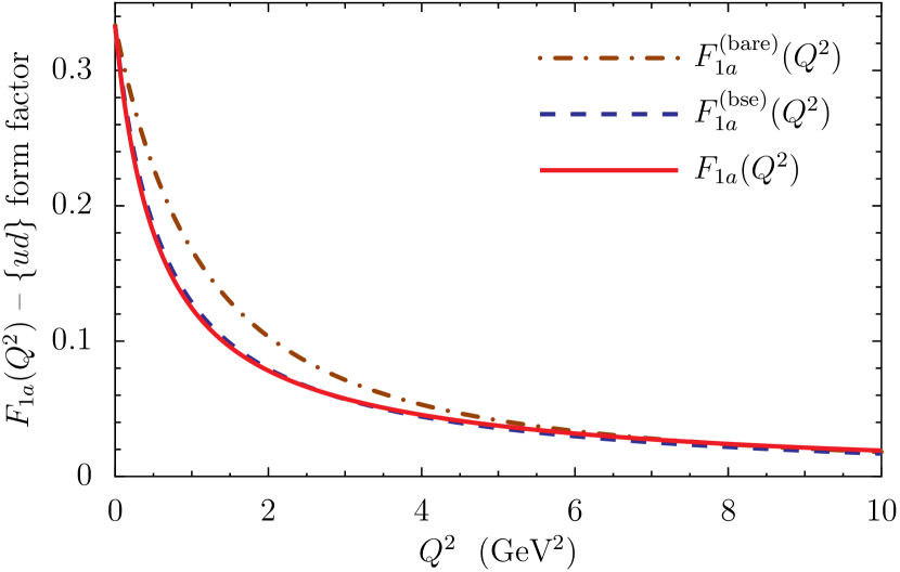
(a)

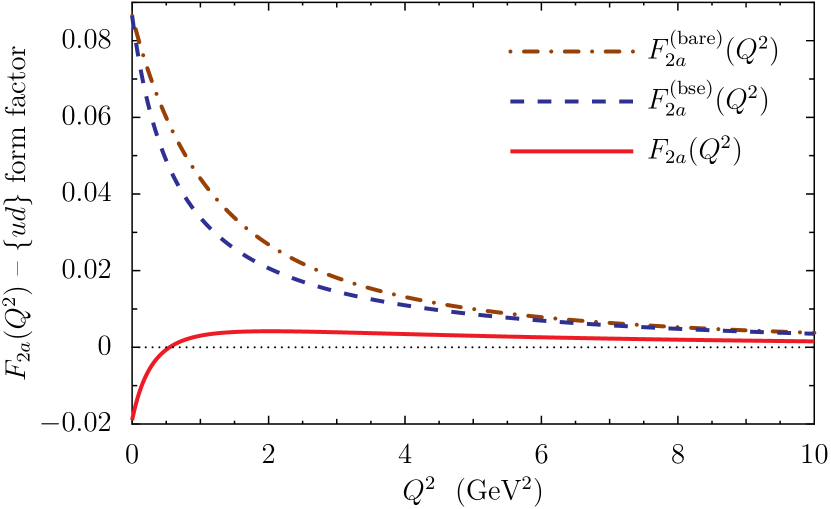
(b)

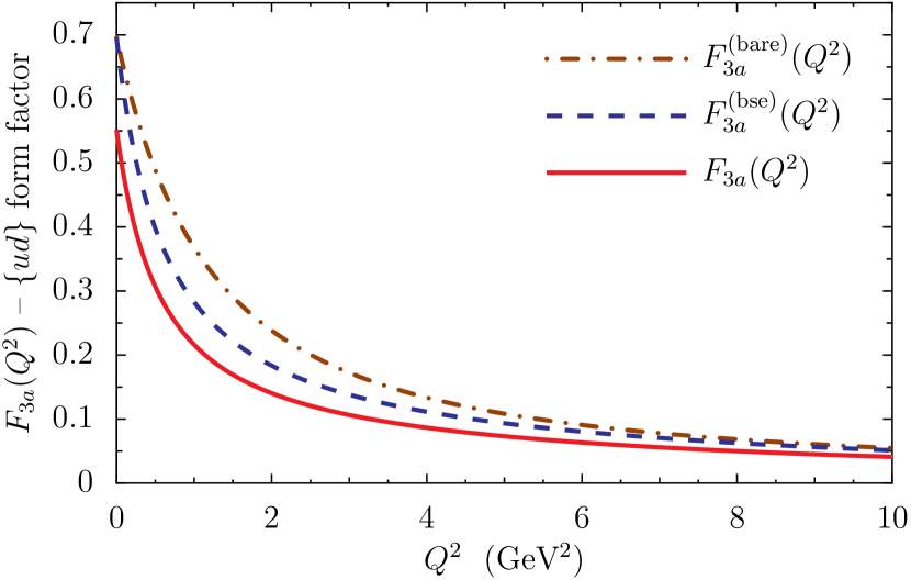
(c)

Figure 15: (Colour online) Form factors for an axialvector diquark with quark content $\{ud\}$.

Results for the form factors of Eq. (88) for an axial–vector diquark with quark content $\{ud\}$ are presented in Figs. 15. In each case the vertex dressing from the quark-photon inhomogeneous BSE results in a softening of form factors, compared to the case of pointlike dressed quarks. Although the pion loop effects leave $F_{1a}$ almost unchanged, both $F_{2a}$ and $F_{3a}$ receive sizeable negative corrections. The origin of these corrections can be traced back to Eq. (88) and the results in Fig. 14. The tensor body from factors $f_{2}^{T}$ and $f_{3}^{T}$ are large and positive for small $Q^{2}$. This, together with the large negative anomalous magnetic moment of the dressed down quark (see Eq. (72)), results in sizeable corrections to $F_{2a}$ and $F_{3a}$ from pion loop effects.

	$\mu^{\text{(bse)}}$	$\mu$		$\mathcal{Q}^{\text{(bse)}}$	$\mathcal{Q}$		$r^{\text{(bse)}}_{C}$	$r_{C}$		$r^{\text{(bse)}}_{M}$	$r_{M}$		$r^{\text{(bse)}}_{Q}$	$r_{Q}$
$\{uu\}$ axialvector diquark	-2.78	-3.14		-1.10	-1.20		0.65	0.76		0.61	0.74		0.61	0.74
$\{ud\}$ axialvector diquark	-0.70	-0.55		-0.28	-0.24		0.37	0.38		0.60	0.62		0.61	0.64
$\{dd\}$ axialvector diquark	-1.39	-2.04		-0.55	-0.73		0.65	0.84		0.61	0.80		0.62	0.79
rho plus	-2.08	-2.57		-0.87	-1.06		0.67	0.82		0.62	0.77		0.62	0.77

Table 3: Results for the magnetic moment, quadruple moment and the charge, magnetic and quadruple radius of the axialvector diquarks and $\rho^{+}$ meson. In each case we present results for various levels of sophistication for the constituent quark form factors. All radii are in units of fm, the magnetic moment has units $e/(2\,m_{H})$ and the quadruple moment $e/m_{H}^{2}$, where $m_{H}$ is the mass of the relevant diquark or meson.

The Lorentz covariant form factors for the $\rho^{+}$ meson, associated with the current of Eq. (88), are given by

$$F_{i\rho}(Q^{2}) =\left[F_{1U}(Q^{2})-F_{1D}(Q^{2})\right]f_{i}^{V}(Q^{2})$$ (93)

$$\,+\left[F_{2U}(Q^{2})-F_{2D}(Q^{2})\right]f_{i}^{T}(Q^{2}),$$ (94)

where $i\in 1,\,2,\,3$ and the body form factors are now functions of the rho mass instead of the axialvector diquark mass. Results for the Sachs-like spin-one form factors defined in Eqs. (89)–(91) are illustrated in Fig. 16 for a $\{ud\}$–type axialvector diquark and the $\rho^{+}$ meson. In these figures we only show the full results which include pion cloud effects. The zero in the charge form factors occurs at $Q^{2}\simeq 6.6\,$GeV² for $G^{\{ud\}}_{C}$ and for $G^{\rho^{+}}_{C}$ at $Q^{2}\simeq 2.6\,$GeV².

Static properties of the $\rho^{+}$ and the axialvector diquarks are given Tab. 3 for variants of the dressed quark form factors. We find that pion loop effects have a substantial impact on the static properties of the axialvector diquarks and rho mesons. For example, the pion cloud increases the magnitude of the $\rho^{+}$ magnetic moment by 24% and the quadrupole moment by 22%, while for the $\{ud\}$–type axialvector diquarks we find a reduction of the magnetic moment by 21% and the magnitude of the quadrupole moment by 14%. The sign difference between these corrections for the $\rho^{+}$ and $\{ud\}$–type axialvector diquark arises because the dressed down quark form factors enter the respective currents with the opposite sign – see Eqs. (92) and (94) – and the dressed down quark has a large anomalous magnetic moment. For the $\rho^{+}$ meson the pion cloud uniformly increases the charge, magnetic and quadrupole radii by approximately 16%, whereas for the $\{ud\}$–type axialvector diquarks the pion cloud has little effect on the charge and quadrupole radii but increases the magnetic radius by 38%.

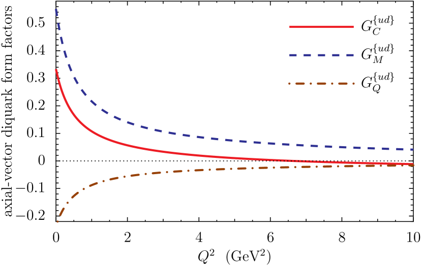
(a)

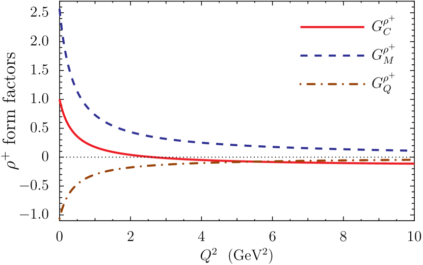
(b)

Figure 16: (Colour online) Upper panel: results for the charge, magnetic and quadruple form factors of a $ud$ axialvector diquark. Lower panel: results for the charge, magnetic and quadruple form factors of a $\rho^{+}$ meson.

As an interesting check on the large $Q^{2}$ behaviour of our rho or axialvector diquark form factor results, we make a comparison with the relations derived in Ref. Brodsky:1992px . That is, at large timelike or spacelike momenta, the ratio of the form factors for a spin-one particle should behave as

$$G_{C}(Q^{2}):G_{M}(Q^{2}):G_{Q}(Q^{2})=\left(1-\tfrac{2}{3}\eta\right):\,2\,:\,-1,$$ (95)

where corrections are of the order $\Lambda_{\text{QCD}}/Q$ and $\Lambda_{\text{QCD}}/M_{\rho}$. For our spin-one results we find that the $G_{C}/G_{Q}$ constraint is satisfied to better than $15\%$ for $Q^{2}=10\,$GeV², to better than $3\%$ for $Q^{2}=100\,$GeV² and for $Q^{2}>1000\,$GeV² our result takes the value given in Eq. (95). The calculated ratios $G_{C}/G_{M}$ and $G_{M}/G_{Q}$ saturate within $15\%$ of the values in Eqs. (95). However this deviation is well within the leading correction of $\Lambda_{\text{QCD}}/M_{\rho}\sim 0.3$.

The remaining diquark electromagnetic current that contributes to the nucleon form factors is the transition current between scalar and axialvector diquarks. This current has the form

$$j^{\mu,\alpha}_{sa}(p^{\prime},p) =\pm\ \frac{1}{M_{s}+M_{a}}\ i\varepsilon^{\alpha\mu\sigma\lambda}p_{\sigma}^{\prime}p_{\lambda}\,F_{sa}(Q^{2}),$$ (96)

where the plus sign indicates a scalar $\to$ axialvector transition and the reverse process has the minus sign. The Lorentz indices $\mu$ and $\alpha$ represent the polarizations of the photon and the axialvector diquark. Evaluating the Feynman diagram of Fig. 11 for this transition process gives

$$F_{sa}(Q^{2}) =\left[F_{1U}(Q^{2})-F_{1D}(Q^{2})\right]f_{sa}^{V}(Q^{2})$$

$$\,+\left[F_{2U}(Q^{2})-F_{2D}(Q^{2})\right]f_{sa}^{T}(Q^{2}),$$ (97)

where $f_{sa}^{V}(Q^{2})$ and $f_{sa}^{T}(Q^{2})$ are the vector and tensor body form factors. The electromagnetic transition form factor describing the $\gamma^{*}\pi^{+}\to\rho^{+}$ process is given by

$$F_{\pi\rho}(Q^{2}) =\left[F_{1U}(Q^{2})+F_{1D}(Q^{2})\right]f_{sa}^{V}(Q^{2})$$

$$\,+\left[F_{2U}(Q^{2})+F_{2D}(Q^{2})\right]f_{sa}^{T}(Q^{2}),$$ (98)

where body form factors are now functions of the $\pi$ and $\rho$ masses. Results for $F_{sa}$ and $F_{\pi\rho}$ are presented in Fig. 17. The vertex dressing from the BSE produces a softer form factor, and for the diquark transition the large isovector combination of the constituent quark Pauli form factors, arising from the pion cloud, gives a sizeable correction for $Q^{2}\lesssim 1\,$GeV². Results for the transition moment and transition radius are given in Tab. 4.

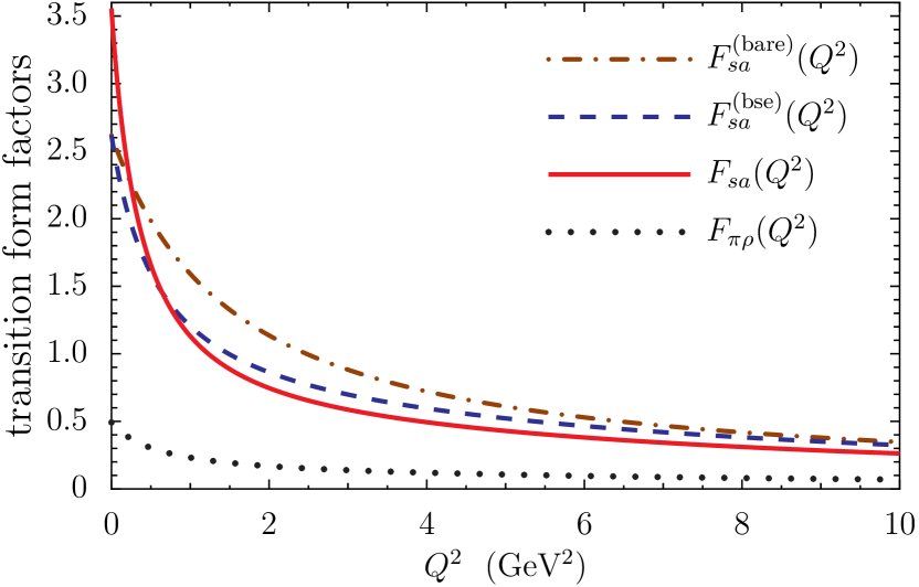
Figure 17: (Colour online) Results for the scalar $\leftrightarrow$ axialvector diquark and $\pi\leftrightarrow\rho$ electromagnetic transition form factors.

	$\kappa_{T}^{\text{(bse)}}$	$\kappa_{T}$		$r_{T}^{\text{(bse)}}$	$r_{T}$
$s\leftrightarrow a$	2.66	3.61		0.75	0.99
$\pi\leftrightarrow\rho$	0.62	0.49		0.54	0.54

Table 4: Results for the transition moment, defined as $\kappa_{T}\equiv F(0)$, the transition radius (which is normalized by $\kappa_{T}$), for scalar $\leftrightarrow$ axialvector diquark and pion $\leftrightarrow$ rho transitions. Radii are in units of fm.

VI Nucleon Form Factor Results

The Feynman diagrams that contribute to the nucleon’s electromagnetic current are illustrated in Fig. 4, where the coupling of the photon to the dressed quarks and diquarks has been discussed in Sects. IV and V, respectively. Using a quark-photon vertex of the form given in Eq. (54) demarcates the nucleon form factors into flavour sectors defined by the dressed quarks, such that

$$F_{ip}(Q^{2}) =F_{ip}^{U}(Q^{2})+F_{ip}^{D}(Q^{2}),$$ (99)

$$F_{in}(Q^{2}) =F_{in}^{U}(Q^{2})+F_{in}^{D}(Q^{2}),$$ (100)

where $i=(1,\,2)$. The dressed quark flavour sector nucleon form factors are given by the product of dressed quark form factors (e.g. Eqs. (67)–(70)) with the nucleon body form factors, such that

$$F_{ip}^{Q} =F_{1Q}\,f_{ip}^{Q,V}+F_{2Q}\,f_{ip}^{Q,T},$$ (101)

$$F_{in}^{Q} =F_{1Q}\,f_{in}^{Q,V}+F_{2Q}\,f_{in}^{Q,T},$$ (102)

where $Q=(U,\,D)$ and the $Q^{2}$ dependence of each form factor has been omitted. The superscript $V$ indicates a vector body form factor and the superscript $T$ a tensor body form factor, which arise from the quark current of Eq. (66).

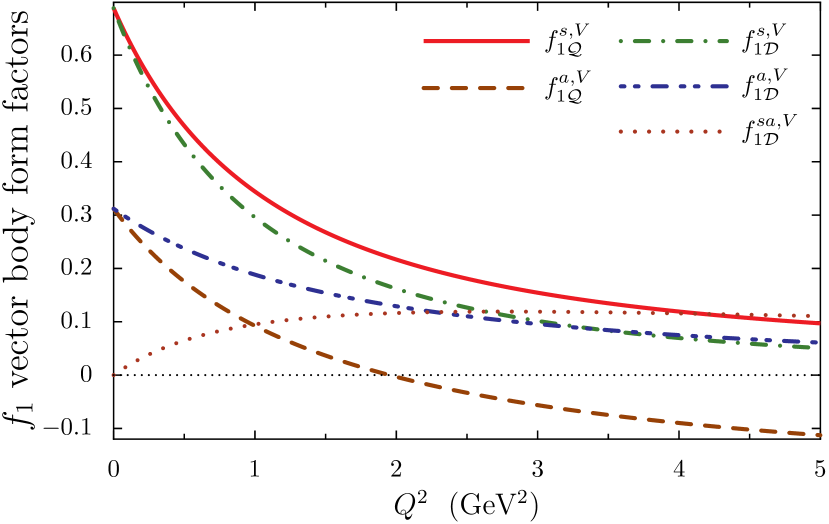
(a)

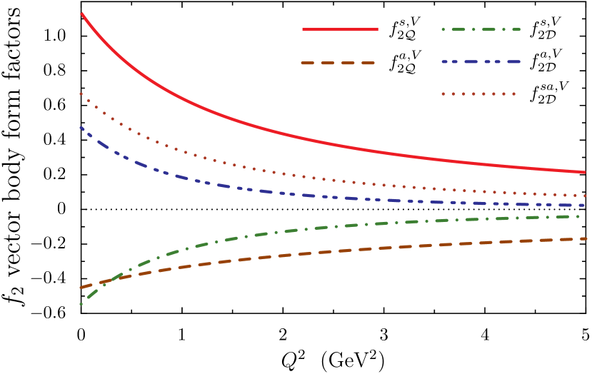
(b)

Figure 18: (Colour online) Nucleon Dirac (upper panel) and Pauli (lower panel) body form factors which result from a vector coupling to the quarks in the Feynman diagrams of Fig. 4. To obtain their contribution to the nucleon form factors these results must be multiplied by the appropriate isospin factors, as in Eqs. (103) and (104), and the dressed quark Dirac form factors.

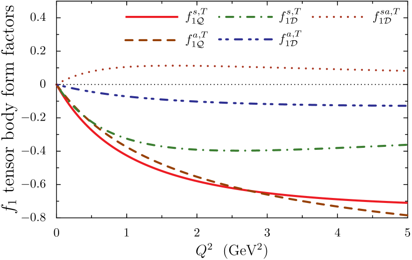
(a)

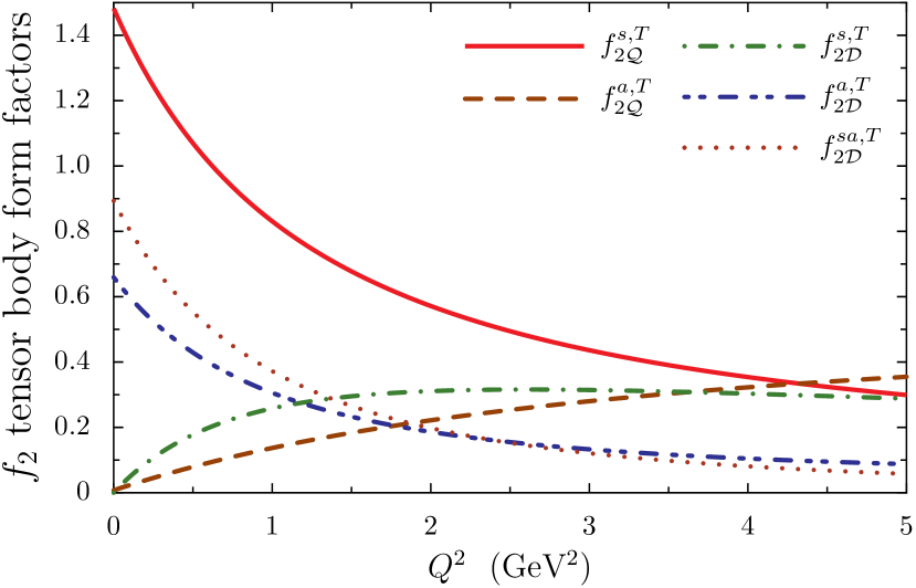
(b)

Figure 19: (Colour online) Nucleon Dirac (upper panel) and Pauli (lower panel) body form factors which result from a tensor coupling to the quarks in the Feynman diagrams of Fig. 4. To obtain their contribution to the nucleon form factors these results must be multiplied by the appropriate isospin factors, as in Eqs. (103) and (104) and the dressed quark Pauli form factors.

	$f^{s,V}_{i\mathcal{Q}}$	$f^{a,V}_{i\mathcal{Q}}$	$f^{s,V}_{i\mathcal{D}}$	$f^{a,V}_{i\mathcal{D}}$	$f^{sa,V}_{i\mathcal{D}}$	$f^{s,T}_{i\mathcal{Q}}$	$f^{a,T}_{i\mathcal{Q}}$	$f^{s,T}_{i\mathcal{D}}$	$f^{a,T}_{i\mathcal{D}}$	$f^{sa,T}_{i\mathcal{D}}$	$f^{U,V}_{ip}$	$f^{D,V}_{ip}$	$f^{U,T}_{ip}$	$f^{D,T}_{ip}$
Dirac	0.688	-0.312	-0.688	0.312	0	0	0	0	0	0	2.00	-1.00	0.00	-0.00
Pauli	1.134	-0.451	-0.546	0.472	0.666	1.482	0.008	0.0	0.659	0.893	1.61	-1.07	3.10	-0.29

Table 5: Nucleon Dirac and Pauli body form factors evaluated at $Q^{2}=0$. The subscript $i=1,2$ corresponds to either the first or second row of the Table. An entry with only one significant figure takes that exact value because of charge conservation. The last four columns give results for the vector and tensor versions of Eqs. (103)–(104) at $Q^{2}=0$. To obtain nucleon form factor results at $Q^{2}=0$ these results must be multiplied the appropriate quark charge for the vector coupling diagrams and by the appropriate dressed quark anomalous magnetic moment for the tensor coupling diagrams.

The proton body form factors in Eq. (101), which represent the sum of the six Feynman diagrams of Fig. 4, have the structure

$$f_{ip}^{U,V} =f^{s,V}_{i\mathcal{Q}}+\tfrac{1}{3}f^{a,V}_{i\mathcal{Q}}+f^{s,V}_{i\mathcal{D}}+\tfrac{5}{3}f^{a,V}_{i\mathcal{D}}+\tfrac{1}{\sqrt{3}}f^{sa,V}_{i\mathcal{D}},$$ (103)

$$f_{ip}^{D,V} =\hskip 31.29802pt\tfrac{2}{3}f^{a,V}_{i\mathcal{Q}}+f^{s,V}_{i\mathcal{D}}+\tfrac{1}{3}f^{a,V}_{i\mathcal{D}}-\tfrac{1}{\sqrt{3}}f^{sa,V}_{i\mathcal{D}}.$$ (104)

For equal current quark masses the neutron body form factors in Eq. (102) are given by

$$f_{in}^{D,V}=f_{ip}^{U,V}\quad\text{and}\quad f_{in}^{U,V}=f_{ip}^{D,V},$$ (105)

and therefore the nucleon body form factors satisfy the constraints imposed by charge symmetry. Expressions for the nucleon tensor body form factors are obtained from Eqs. (103)–(105) with $V\to T$. The nomenclature for these nucleon body form factors is: a subscript $\mathcal{Q}$ implies that the photon couples directly to a quark (quark diagram) and a subscript $\mathcal{D}$ implies that the photon couples to (a quark inside) a diquark (diquark diagram); a superscript $s$ indicates that the diagram contains only a scalar diquark, while the superscript $a$ only an axialvector diquark and the superscript $sa$ implies the sum of the two diagrams where a photon induces a transition between scalar and axialvector diquarks. The numerical coefficients in Eqs. (103) and (104) arise from the isospin structure of the proton Faddeev and the quark-photon vertices, given in Eqs. (30) and (54), respectively.

Nucleon body form factor results for each diagram in Fig. 4, as expressed by Eqs. (103)–(104), are presented in Fig. 18 for the vector coupling to the dressed quarks and in Fig. 19 for the tensor coupling. Table 5 gives the $Q^{2}=0$ values of the nucleon body form factors. Charge conservation for the vector coupling implies that in this case diagrams with the same quark–diquark content must be equal at $Q^{2}=0$. Furthermore, with the normalization used here, the sum of quark diagrams and of diquark diagrams must each equal one in the vector case. For the vector coupling, charge conservation also forbids the scalar–axialvector diquark diagram ($sa$) from contributing to the charge. However, this diagram does give an important contribution to the nucleon anomalous magnetic moment. For the vector coupling diagrams the only object with a magnetic moment is the axialvector diquark. Thus the non-zero values for the other $f_{2}$ body form factor diagrams, in the lower panel of Fig. 18, indicate that the associated pieces of the nucleon wave function have sizable $p$ and $d$ wave components. Therefore the nucleon wave function contains a significant amount of quark orbital angular momentum.

Figure 19 and Table 5 demonstrate that the tensor coupling diagrams do not contribute to the nucleon charge, which is consistent with constraints imposed by the Ward–Takahashi identity for the nucleon electromagnetic current. However, these diagrams do have an important impact on the anomalous magnetic moment. The $Q^{2}$ behavior of the form factors is also influenced by the tensor coupling diagrams. However, once multiplied by the dressed quark Pauli form factors, their contribution diminishes rapidly with $Q^{2}$, being of little importance for $Q^{2}\gtrsim 1\,$GeV².

In Sect. II the nucleon Faddeev equation was solved by first making a pole approximation for the diquark $t$-matrices – see for example Eqs. (38) and (39). For a consistent nucleon form factor calculation we must therefore approximate all two-body $t$-matrices by their pole form, which also includes the quark-photon vertex obtained from the inhomogeneous BSE illustrated in Fig. 5. Expressing $\Pi_{VV}(q^{2})=q^{2}\,\hat{\Pi}_{VV}(q^{2})$ in Eq. (60) and expanding $\hat{\Pi}_{VV}(q^{2})$ about either the rho or omega pole mass, we obtain the following results for the pole forms of the BSE form factors:

$$F_{1i}(Q^{2}) =\frac{1}{1+Q^{2}/m_{i}^{2}},\qquad i\in\omega,\,\rho,$$ (106)

which is the familiar vector meson dominance result. The dressed quark form factors therefore maintain the vector meson pole structure in the time-like region obtained in the original BSE results of Eq. (60). For the nucleon form factor calculations the result in Eq. (106) will replace the full BSE result of Eq. (60) used in the dressed quark form factors, for example, in Eq. (61) and Eqs. (67)–(70).

Dirac and Pauli form factor results for the proton and neutron are presented in Fig. 20 and 21, respectively, while results for the Sachs form factors are given in Fig. 22 and 23. The three curves in each figure represent results for the three variants of the dressed quark form factors used in Eqs. (99)–(102). The dot-dashed curve is the result where the dressed quarks are treated as pointlike and therefore their Dirac form factors are constants equal to the quark charges and the Pauli form factors are zero. These results are labelled with the superscript (bare). Results for the nucleon form factors that include the dressing of the quark-photon vertex by vector mesons, generated by Eq. (106), are illustrated by the dashed lines, with the superscript (bse). Finally, we use dressed quark form factors that also incorporate effects from pion loops, which generate a non-zero Pauli form factor for the dressed quarks. These results are illustrated as the solid lines (without a superscript label).

The full results for the nucleon form factors, including pion loop effects, display good agreement with the empirical parametrizations from Ref. Kelly:2004hm , which are illustrated as the dotted curves in Figs. 20 through 23. Both the proton and neutron Dirac form factor are slightly softer than the empirical parametrizations, whereas the Pauli form factors are in almost perfect agreement. The dressing of the quark-photon vertex by the pole form of the BSE (Eq. (106)) results in a significant softening of all nucleon form factors, proving critical for a realistic $Q^{2}$ dependence of the form factors. Pion loop corrections result in a further 50% reduction of the neutron Dirac form factor for low to moderate $Q^{2}$ and significantly enhance the nucleon Pauli form factors for $Q^{2}\lesssim 1\,$GeV². These enhancements correspond to increases in the magnitude of the proton and neutron anomalous magnetic moments by $25\%$ and $45\%$, as indicated in Table 6. For the proton and neutron magnetic moments we find $\mu_{p}=2.78\,\mu_{N}$ and $\mu_{n}=-1.81\,\mu_{N}$, which agree well with the experimental values of $\mu_{p}=2.793\,\mu_{N}$ and $\mu_{n}=-1.913\,\mu_{N}$ Beringer:1900zz . To obtain the physical result $\left|\kappa_{n}\right|>\kappa_{p}$ for the nucleon anomalous magnetic moments, we find that the dressed quark anomalous magnetic moments of Eq. (72) are critical. In particular, $\kappa_{U}$ must be positive and $\kappa_{D}$ negative, with $\left|\kappa_{D}\right|>\kappa_{U}$. We obtain $\left|\kappa_{D}\right|>\kappa_{U}$ because the second diagram in Fig. 8 only contributes to the dressed down quark anomalous magnetic moment (c.f. Eqs. (69) and (70)), giving an additional negative contribution.

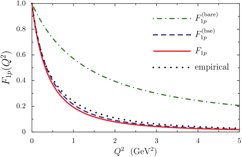
(a)

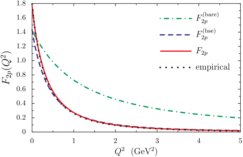
(b)

Figure 20: (Colour online) Results for the proton Dirac (upper panel) and Pauli (lower panel) form factors. In each case the dot-dashed curve (superscript (bare)) gives the result when the constituent quark form factors are those of an elementary Dirac particle, the dashed curve (superscript (bse)) includes the quark-photon vertex dressing effects from the BSE and the solid curve is the full result which also includes pion loop effects. The dotted curve is the empirical result from Ref. Kelly:2004hm .

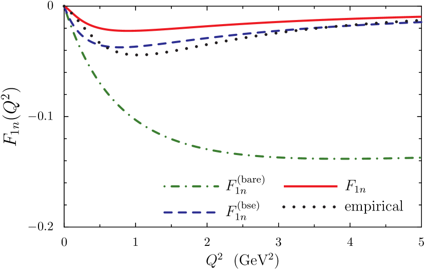
(a)

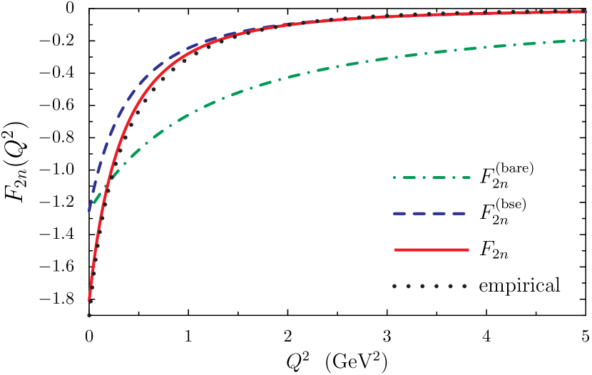
(b)

Figure 21: (Colour online) Results for the neutron Dirac (upper panel) and Pauli (lower panel) form factors. In each case the dot-dashed curve (superscript (bare)) gives the results when the constituent quark form factors are those of an elementary Dirac particle, the dashed curve (superscript (bse)) includes the quark-photon vertex dressing effects from the BSE and the solid curve is the full result which also includes pion loop effects. The dotted curve is the empirical result from Ref. Kelly:2004hm .

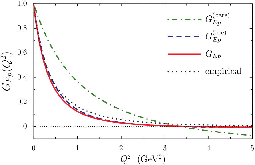
(a)

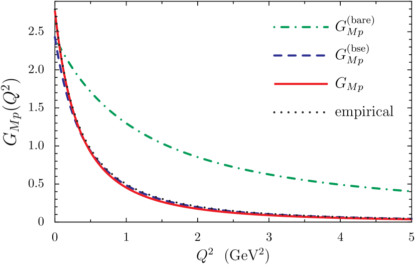
(b)

Figure 22: (Colour online) Results for the proton Sachs electric (upper panel) and magnetic (lower panel) form factors. In each case the dot-dashed curve (superscript (bare)) is the result when the constituent quark form factors are those of an elementary Dirac particle, the dashed curve (superscript (bse)) includes the quark-photon vertex dressing effects from the BSE and the solid curve is the full result which also includes pion loop effects. The dotted curve is the empirical result from Ref. Kelly:2004hm .

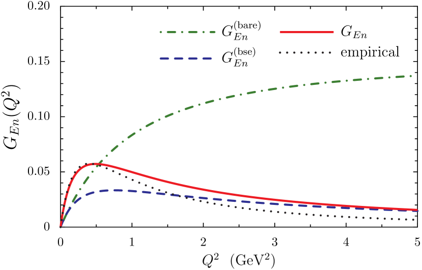
(a)

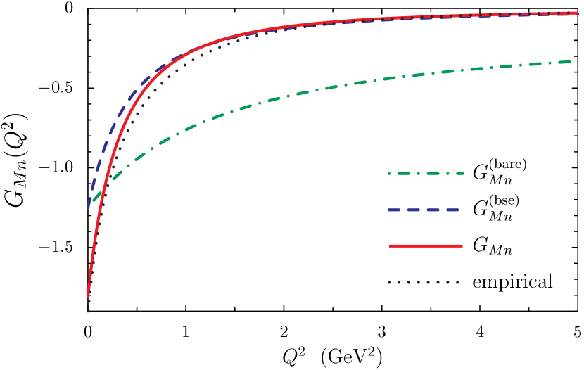
(b)

Figure 23: Colour online) Results for the neutron Sachs electric (upper panel) and magnetic (lower panel) form factors. In each case the dot-dashed curve (superscript (bare)) is the results when the constituent quark form factors are those of an elementary Dirac particle, the dashed curve (superscript (bse)) includes the quark-photon vertex dressing effects from the BSE and the solid curve is the full result which also includes pion loop effects. The dotted curve is the empirical result from Ref. Kelly:2004hm .

Results for the charge and magnetic radii, defined by Eqs. (49) and (50), are given in Table 6 for the two cases where the dressed quark form factors are given by Eq. (106) and where pion loop effects are also included. The pion loop effects result in a $65\%$ increase in magnitude of the neutron charge radius, a $19\%$ increase in its magnetic radius, while the proton charge radius increases by 6% and the magnetic radius by 12%. All nucleon radii agree well with the empirical values taken from Ref. Kelly:2004hm . A recent global fit to data Zhan:2011ji found the proton charge and magnetic radius to be

$$r_{Ep} =0.875\pm 0.008(\text{exp})\pm 0.006(\text{fit})\leavevmode\nobreak\ \text{fm},$$ (107)

$$r_{Mp} =0.867\pm 0.009(\text{exp})\pm 0.018(\text{fit})\leavevmode\nobreak\ \text{fm},$$ (108)

and a recent Mainz experiment found Bernauer:2010wm

$$r_{Ep} =0.879\phantom{1}(5)_{\text{stat}}(4)_{\text{syst}}(2)_{\text{model}}(4)_{\text{group}}\leavevmode\nobreak\ \text{fm},$$ (109)

$$r_{Mp} =0.777(13)_{\text{stat}}(9)_{\text{syst}}(5)_{\text{model}}(2)_{\text{group}}\leavevmode\nobreak\ \text{fm}.$$ (110)

Our proton results agree well with those of Ref. Zhan:2011ji . The origin of the sizeable discrepancy between the two experimental results for the proton magnetic radius is discussed, for example, in Ref. Sick:2012zz . In addition, in view of the muonic hydrogen controversy Pohl:2010zza , the experimental errors quoted in both places appear to be rather low.

	$\mu^{\text{(bse)}}$	$\mu$	$\mu^{\text{exp}}$		$r_{E}^{\text{(bse)}}$	$r_{E}$	$r_{E}^{\text{exp}}$		$r_{M}^{\text{(bse)}}$	$r_{M}$	$r_{M}^{\text{exp}}$
proton	-2.43	-2.78	-2.793		-0.81	-0.86	-0.863$\pm$0.004		0.76	0.84	0.848$\pm$0.003
neutron	-1.25	-1.81	-1.913		-0.20	-0.34	-0.335$\pm$0.055		0.74	0.88	0.907$\pm$0.016

Table 6: Results for the nucleon magnetic moments and radii, with dressed quark form factors given by Eqs. (61) and (106), labelled with a superscript (bse), and results that also include pion cloud effects at the dressed quark level (these results do not carry a superscript label). Experimental results, labelled with a superscript exp, are taken from Ref. Kelly:2004hm .

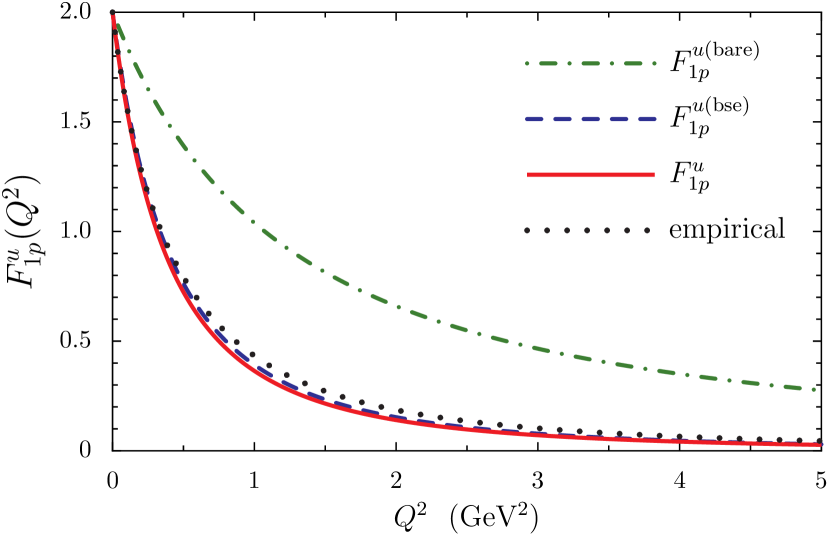
(a)

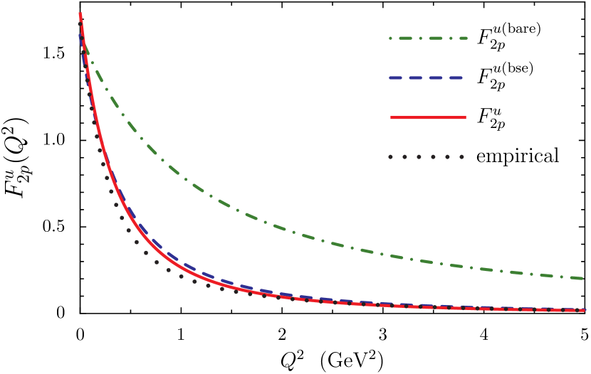
(b)

Figure 24: (Colour online) Proton up quark sector Dirac and Pauli form factors. The empirical results are obtained using Ref. Kelly:2004hm and Eq. (47).

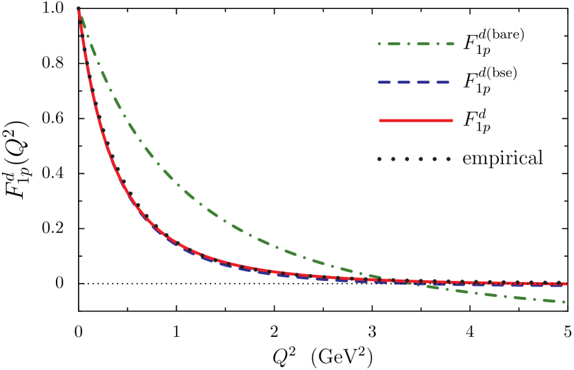
(a)

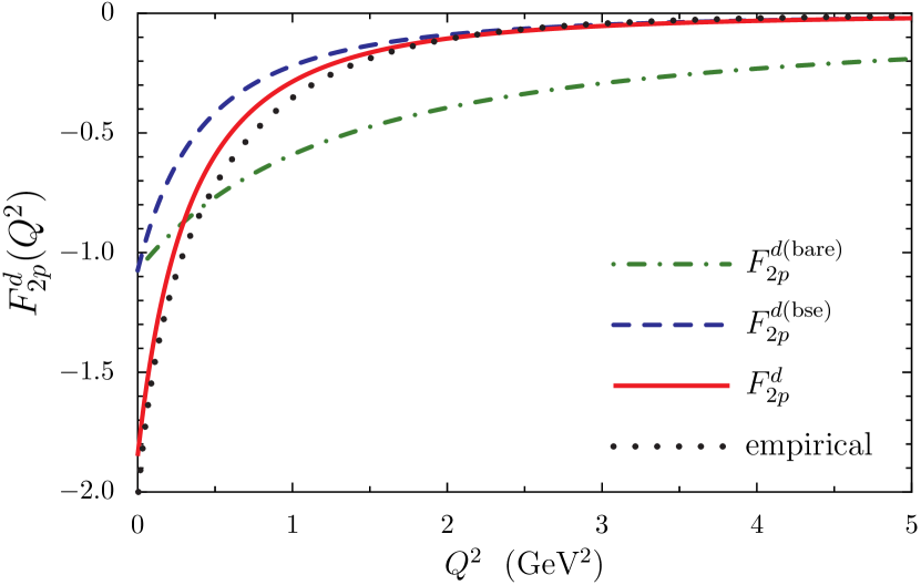
(b)

Figure 25: (Colour online) Proton down quark sector Dirac and Pauli form factors. The empirical results are obtained using Ref. Kelly:2004hm and Eq. (47).

The flavour sector nucleon form factors defined by the dressed quarks, as given in Eqs. (101)–(102), do not satisfy the standard charge symmetry relations, that is

$$\frac{F^{U}_{ip}}{e_{u}} \neq\frac{F^{D}_{in}}{e_{d}} \frac{F^{D}_{ip}}{e_{d}} \neq\frac{F^{U}_{in}}{e_{u}}.$$ and (111)

where $i=(1,\,2)$. The reason for this lies not with the nucleon body form factors, c.f. Eq. (105), but with the form factors of the dressed quarks. Dressed quarks are quasi-particles that contain an infinite number of $u$ and $d$ current quarks. Hence a dressed up quark form factor, for example, contains contributions from both $u$ and $d$ current quarks. To obtain the nucleon quark sector form factors, defined in general in Eq. (43), the dressed quark form factors must be expressed in their quark sector form as given in Eqs. (77)–(80). The nucleon quark sector form factors are therefore given by

$$F^{q}_{ip} =F_{1Q}^{q}\,f_{ip}^{Q,V}+F_{2Q}^{q}\,f_{ip}^{Q,T},$$ (112)

$$F^{q}_{in} =F_{1Q}^{q}\,f_{in}^{Q,V}+F_{2Q}^{q}\,f_{in}^{Q,T},$$ (113)

where $i=(1,\,2)$, $q=(u,\,d)$ and there is an implied sum over $Q=(U,\,D)$. These results satisfy the charge symmetry constraints

$$F^{u}_{in} =F^{d}_{ip} F^{d}_{in} =F^{u}_{ip}.$$ and (114)

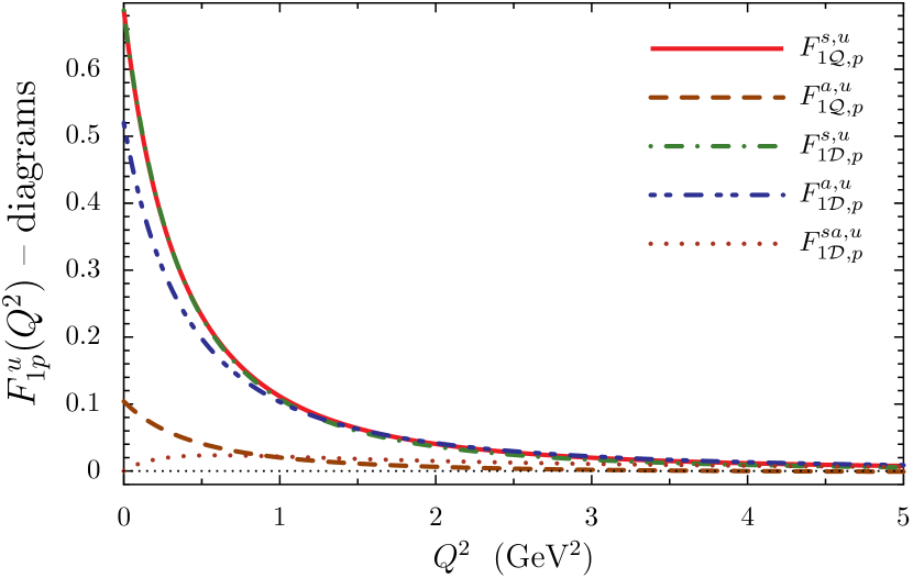
(a)

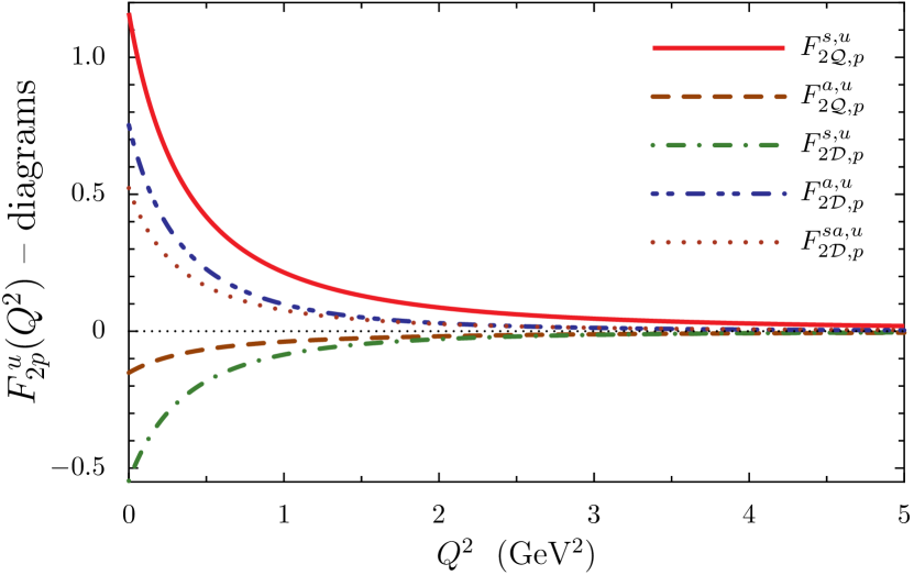
(b)

Figure 26: (Colour online) Total contributions to the proton $u$-sector form factors from each Feynman diagram in Fig. 4. These results include both the vector and tensor coupling contributions and the sum gives the total $u$-sector Dirac and Pauli proton form factors (solid lines in Fig. 24).

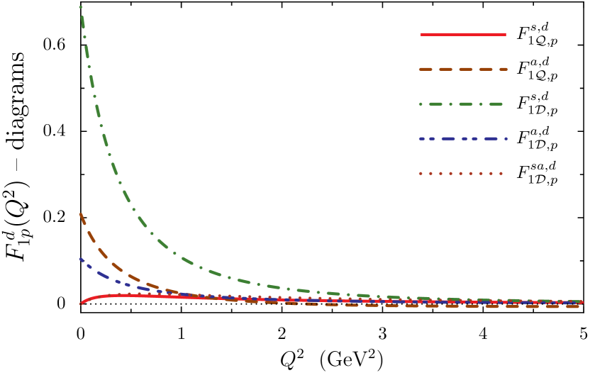
(a)

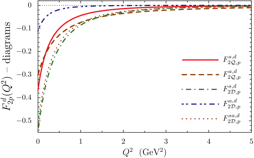
(b)

Figure 27: (Colour online) Total contributions to the proton $d$-sector form factors from each Feynman diagram in Fig. 4. These results include both the vector and tensor coupling contributions and the sum gives the total $d$-sector Dirac and Pauli proton form factors (solid lines in Fig. 25).

$q$	$\kappa^{q,\text{(bse)}}$	$\kappa^{q}$	$\kappa^{q,\text{exp}}$		$r_{E}^{q,\text{(bse)}}$	$r_{E}^{q}$	$r_{E}^{q,\text{exp}}$		$r_{M}^{q,\text{(bse)}}$	$r_{M}^{q}$	$r_{E}^{q,\text{exp}}$
$u$ sector	-1.61	-1.74	-1.673		0.79	0.82	0.829$\pm$0.097		-0.77	0.83	0.816$\pm$0.087
$d$ sector	-1.07	-1.85	-2.033		0.75	0.71	0.720$\pm$0.118		-0.53	0.98	1.048$\pm$0.319

Table 7: Results for the quark sector contribution to the proton anomalous magnetic moments and radii, with constituent quark form factors given by Eqs. (61) and (106) (labelled with (bse)) and results that also include the pion cloud. The experimental values for the quark sector anomalous magnetic moments and radii are obtained from from Ref. Kelly:2004hm using Eq. (47).

Quark sector proton form factor results are presented in Figs. 24 and 25, for the three stages of sophistication in the description of the dressed quark form factors. Empirical results, shown by the dotted line, were obtained from Ref. Kelly:2004hm using Eq. (47). While the agreement between our full results, which include pion loop effects, and the empirical parametrization is very good, for the $u$ quark sector we find that our Dirac form factor is slightly too soft and the Pauli form factor a little too hard. For the $d$ quark sector the Dirac form factor is in excellent agreement with the empirical parametrization, whereas the Pauli form factor is slightly too soft. As we shall see, such small differences can produce apparently large effects in the combination required to compute $G_{E}$.

	$r_{1}^{\text{(bse)}}$	$r_{1}$	$r_{1}^{\text{exp}}$	$r_{2}^{\text{(bse)}}$	$r_{2}$	$r_{2}^{\text{exp}}$		$r_{1}^{q,\text{(bse)}}$	$r_{1}^{q}$	$r_{1}^{q,\text{exp}}$	$r_{2}^{q,\text{(bse)}}$	$r_{2}^{q}$	$r_{2}^{q,\text{exp}}$
proton	0.75	0.79	0.791	0.77	0.85	0.879	$u$-sector	0.76	0.79	0.795	0.77	0.88	0.841
neutron	0.20	0.09	0.119	0.76	0.88	0.911	$d$-sector	0.80	0.80	0.809	0.76	0.88	0.938

Table 8: Results for radii defined by Eq. (48), for the proton and neutron Dirac and Pauli form factors, and for the quark sector proton Dirac and Pauli form factors. In each case we show results where the dressed quark form factors are given by Eqs. (61) and (106) (labelled with (bse)) and results that also include the pion cloud. The empirical values are obtained from Ref. Kelly:2004hm and for the quark sector results using Eq. (47).

An interesting feature of these results is the role of the pionic corrections to the quark sector Pauli form factors. In contrast to the usual proton and neutron Pauli form factors, which each receive significant corrections from the pion cloud, for the quark sector form factors only $F^{d}_{2p}$ receives sizeable pionic corrections. For example, pion loop effects increase the magnitude of the $d$ sector anomalous magnetic moment by 73%, whereas the $u$ quark sector only receives an 8% correction. This result is a consequence of the Pauli quark sector form factors for the dressed quarks, where from Eq. (82) we see that the $d$ quark sector contribution to the dressed up quark anomalous magnetic moment has a magnitude twelve times larger than the $u$ sector contribution, and the proton consists of two dressed up quarks and one dressed down quark. When compared with experiment the $d$-sector anomalous magnetic moment is 10% too small and the $u$-sector 4% too large.

Table 7 presents results for the quark sector contribution to the proton anomalous magnetic moments and radii. We find that the pion cloud has only a minor impact on the $d$-sector charge radius and the $u$-sector radii, whereas the $d$-sector magnetic radius actually changes sign once pion loop effects are included. Again the origin of this lies with the large value of $\kappa_{U}^{d}$ in Eq. (82). With pion cloud corrections included, all our results for the charge and magnetic quark sector radii agree well with experiment.

Table 8 gives results for the Dirac and Pauli radii, defined by Eq. (48), for the proton and neutron and, for the proton, the corresponding quark sector radii. The agreement with the empirical results of Ref. Kelly:2004hm is very good for the proton and neutron radii. For the proton quark sector radii, the Dirac radii results are in good agreement; however, the $u$ quark sector Pauli radius is slightly larger than experiment and the $d$ quark sector is 7% smaller.

$q$	$F^{s,q}_{1\mathcal{Q},p}$	$F^{a,q}_{1\mathcal{Q},p}$	$F^{s,q}_{1\mathcal{D},p}$	$F^{a,q}_{1\mathcal{D},p}$	$F^{sa,q}_{1\mathcal{D},p}$	$F^{q}_{1p}$	$F^{s,q}_{2\mathcal{Q},p}$	$F^{a,q}_{2\mathcal{Q},p}$	$F^{s,q}_{2\mathcal{D},p}$	$F^{a,q}_{2\mathcal{D},p}$	$F^{sa,q}_{2\mathcal{D},p}$	$F^{q}_{2p}$
$u$-sector	0.69	0.10	0.69	0.52	0	2	-1.16	-0.15	-0.55	-0.75	-0.52	-1.73
$d$-sector	0	0.21	0.69	0.10	0	1	-0.37	-0.30	-0.55	-0.11	-0.52	-1.85

Table 9: Contributions to the nucleon quark-sector form factors from the various diagrams at $Q^{2}=0$. The vector contributions are obtained from the appropriate body form factors at $Q^{2}=0$ multiplied by isospin factors and quark charges. Therefore these results do not change with the various approximations for the dressed quark form factors. The tensor contributions are only non-zero if the dressed quarks have an anomalous magnetic moment, and in this framework this occurs solely from pion loop effects. Rows with an entry of “0” are identically zero because of charge conservation.

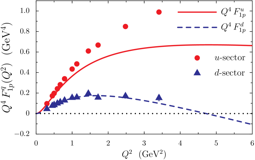
Figure 28: (Colour online) Quark sector contributions to the proton Dirac form factor multiplied by $Q^{4}$. Experimental data are taken from Ref. Cates:2011pz .

Figures 26 and 27 present results for the total contribution of each diagram in Fig. 4 to the proton quark sector form factors. That is, the proton quark sector form factors are decomposed into

$$F^{q}_{ip} =F^{s,q}_{i\mathcal{Q},p}+F^{a,q}_{i\mathcal{Q},p}+F^{s,q}_{i\mathcal{D},p}+F^{a,q}_{i\mathcal{D},p}+F^{sa,q}_{i\mathcal{D},p},$$ (115)

where $i=(1,\,2)$, $q=(u,\,d)$ and each function represents the total contribution to each quark sector for the Feynman diagrams in Fig. 4. Table 9 gives results for the quark sector diagrams of Fig. 4 evaluated at $Q^{2}=0$. For the Dirac form factors we see the dominance of the scalar diquark in the proton wave function, where these diagrams carry 69% of both the $u$ and $d$ quark sector charges. Axialvector diquarks also play an important role for the $u$ quark sector form factors, carrying 26% of the charge and 35% of the anomalous magnetic moment. In the $d$ quark sector, $F^{s,d}_{2\mathcal{Q},p}$ would be zero without the effect of the pion cloud. The latter produces a contribution that constitutes 20% of the $d$ sector anomalous magnetic moment.

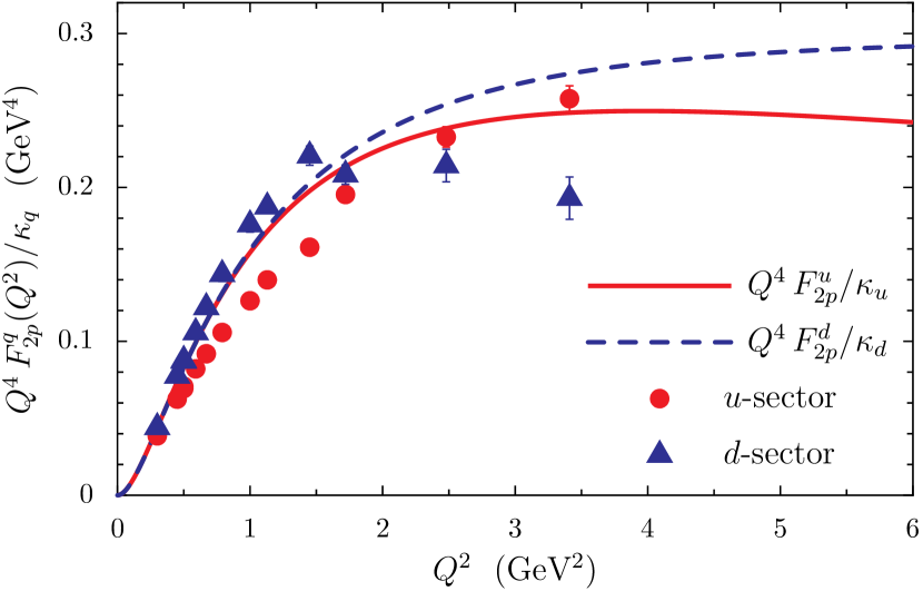
Figure 29: (Colour online) Quark sector contributions to the proton Pauli form factor multiplied by $Q^{4}$. Experimental data are taken from Ref. Cates:2011pz .

Recent accurate neutron form factor data has enabled a precise experimental determination of the quark sector proton form factors, using Eq. (44). The experimental quark sector results from Ref. Cates:2011pz , along with our results, are presented in Fig. 28 for the Dirac form factors and in Fig. 29 for the Pauli form factors. Prima facie, these experimental results are remarkable. For $Q^{2}$ beyond 1-2 GeV² the $d$ quark sector of the proton Dirac form factor is much softer than the $u$ quark sector. On the other hand, for the Pauli quark sector form factors, it is the $u$ quark sector that is softer for low $Q^{2}$. However, at around $Q^{2}\sim 1.5\,$GeV² there is a cross-over and the $d$ quark sector form factor starts approaching zero more rapidly.

The empirical results illustrated in Fig. 28 are straightforward to understand within our framework. The dominant contributions to the quark sector Dirac form factors come from the two Feynman diagrams which involve only a quark and a scalar diquark. This is clear from the upper panels of Figs. 26 and 27. The upper panel in Figs. 10 demonstrates that the current $d$ quarks that contribute to $F_{1p}^{d}$ must primarily come from the dressed down quark, and these contributions are suppressed by order $1/Q^{2}$ relative to the current $u$ quarks from the quark diagram that contributes to $F_{1p}^{u}$. Thus the dominance of scalar diquark correlations in the nucleon clearly provides a very natural explanation of the data in Fig. 28.

The zero-crossing in our result for $F_{1p}^{d}$ at $Q^{2}\simeq 4.7\,$GeV² is also straightforward to understand. We first note that the large $Q^{2}$ behaviour of the form factors is governed by the quark diagrams in Fig. 4, because when the photon couples to a quark inside a diquark, the diquark form factors provide at least an additional factor of $1/Q^{2}$ relative to the quark diagrams. Considering only pointlike quarks, which is sufficient to study the large $Q^{2}$ behaviour, we have for the proton quark sector form factors

$$F_{ip}^{u} \leavevmode\nobreak\ \stackrel{{\scriptstyle Q^{2}\to\infty}}{{\longrightarrow}}\leavevmode\nobreak\ f^{s,V}_{i\mathcal{Q}}+\tfrac{1}{3}f^{a,V}_{i\mathcal{Q}},$$ (116)

$$F_{ip}^{d} \leavevmode\nobreak\ \stackrel{{\scriptstyle Q^{2}\to\infty}}{{\longrightarrow}}\leavevmode\nobreak\ \hskip 31.29802pt\tfrac{2}{3}f^{a,V}_{i\mathcal{Q}},$$ (117)

where $i=(1,\,2)$; c.f. Eqs. (103) and (104). Therefore the large $Q^{2}$ behaviour of $F_{1p}^{d}$ is governed by the nucleon body form factor $f^{a,V}_{1\mathcal{Q}}$ (see Fig. 18), which becomes negative at large $Q^{2}$ and therefore $F_{1p}^{d}$ has a zero-crossing. Note that the empirical parameterizations of Ref. Kelly:2004hm also have a zero in $F_{1p}^{d}$ at $Q^{2}\simeq 7.9\,$GeV².

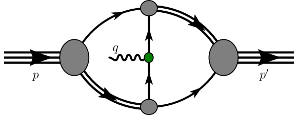
(a)

Figure 30: Exchange type diagrams that do not appear in our present form factor calculation because the static approximation is used for the quark exchange kernel.

Understanding the $Q^{2}$ dependence of the proton Pauli quark sector form factors is more subtle within our model. Analogous to the Dirac form factor example, $F_{2p}^{u}$ receives a large contribution from the scalar quark diagram $f^{s,V}_{2\mathcal{Q}}$, however, many other contributions are negative. In contrast all diagrams add constructively to the $F_{2p}^{d}$ form factor, which also receives a significant contribution from the pion cloud. Therefore at low to moderate $Q^{2}$ we find $F_{2p}^{u}/\kappa_{u}\sim F_{2p}^{d}/\kappa_{d}$, with reasonable agreement with the data. However, at larger $Q^{2}$ the two quark diagrams in Eq. (116) partially cancel, giving $F_{2p}^{u}/\kappa_{u}<F_{2p}^{d}/\kappa_{d}$, which is opposite to the behaviour observed in the data. The suppression of $F_{2p}^{d}$ with respect to $F_{2p}^{u}$ at large $Q^{2}$ was found in Ref. Cloet:2008re , where a major difference from the framework used here is that we make the static approximation to the quark exchange kernel and therefore exchange type diagrams, as illustrated in Fig. 30, are absent from our form factor calculation. This is the likely reason for the discrepancy with experiment at large $Q^{2}$ observed in Fig. 29.

Detailed results for the proton and neutron Sachs form factors are given in Appendix C. Of contemporary interest is the proton Sachs form factor ratio, $G_{Ep}/G_{Mp}$, for which our result is presented in Fig. 31. We find that this ratio decreases almost linearly with $Q^{2}$ but the slope we obtain is significantly larger than the experimental results obtained via the polarization transfer experiments, leading to a zero-crossing at $Q^{2}\approx 3.7$ GeV². So far no such zero-crossing has been seen in the data but if it were to occur it would have to be in the domain $Q^{2}\gtrsim 8\,$GeV². The zero in the $G_{Ep}/G_{Mp}$ ratio found here results from a zero in $G_{Ep}$ and, as we have already noted, the cancellation between $F_{1}$ and $F_{2}$ in the linear combination needed for $G_{E}$ means that even relatively small differences between the experimental and theoretical values of the individual from factors can be magnified there. We find that this zero actually arises from the $u$ quark sector, as illustrated in the upper panel of Fig. 33. This zero has its origin in the quark diagram with the scalar diquark spectator, which becomes negative at around $Q^{2}\simeq 1.8\,$GeV² and dominates at large $Q^{2}$. This can be seen in the upper panel of Fig. 35. A possible reason for the discrepancy with data for the $G_{Ep}/G_{Mp}$ ratio is the omission of exchange diagram contributions (illustrated in Fig. 30), which do not appear in the model described herein. The running of the quark mass function in QCD may also play an important role Cloet:2013gva .

Results for the neutron Sachs form factor ratio, $G_{En}/G_{Mn}$, are presented in Fig. 32. For $Q^{2}\lesssim 1.5\,$GeV² our results that include pion loop corrections agree well with data. However, at larger $Q^{2}$ our ratio continues to grow too rapidly to be consistent with data. Our result for $G_{En}/G_{Mn}$ does not possess a zero-crossing for any $Q^{2}$ value. This is in contrast to the results of Ref. Cloet:2008re which find a zero-crossing at $Q^{2}\simeq 11\,$GeV².

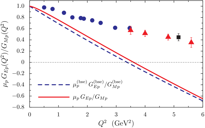
Figure 31: (Colour online) Proton Sachs form factor ratio. Data are from Refs. Jones:1999rz ; Gayou:2001qd ; Gayou:2001qt ; Puckett:2010ac ; Puckett:2011xg .

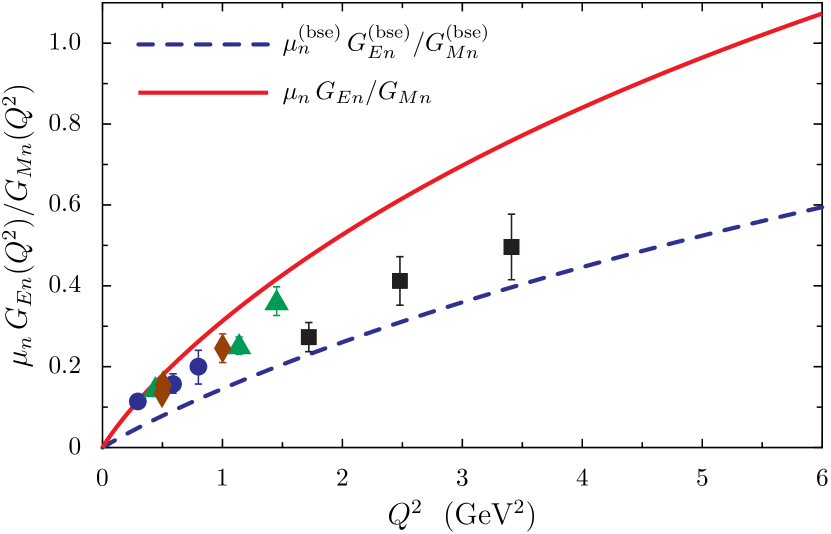
Figure 32: (Colour online) Neutron Sachs form factor ratio. Data are from Refs. Riordan:2010id .

VII Conclusion

We have presented calculations of the nucleon form factors using a covariant and confining NJL model, which is a Poincaré covariant quantum field theory with many of the properties of QCD at low to moderate energies. The model satisfies current conservation exactly and because the framework is covariant the form factors are determined without the need to specify a reference frame. Poincaré covariance also demands non-zero quark orbital angular momentum in the proton wave function, and this is reflected in our results by large contributions to the nucleon Pauli form factors from quark-diquark components of the nucleon wave function that only carry charge (see Fig. 18 and related discussion).

A unique feature of these results is the parameter-free self-consistent inclusion of pion loop effects, as a perturbation to the “quark core” results obtained from the solution of a relativistic Faddeev equation. These pion cloud effects play a vital role for $Q^{2}\lesssim 1\,$GeV². For example, the pion cloud increases the magnitude of the proton and neutron anomalous magnetic moments by 25% and 45%, respectively, giving final results of $\kappa_{p}=1.78$ and $\kappa_{n}=-1.81$, which are in rather good agreement with the empirical values.

In the limit of equal current quark masses our model satisfies charge symmetry and therefore the proton quark sector form factors can be unambiguously determined. For the quark sector radii we find that $r^{u}_{E}$ is 16% larger than $r^{d}_{E}$, whereas for the magnetic radii $r^{d}_{M}$ is 18% larger than $r^{u}_{M}$. The quark sector magnetic radius result can be understood because pion loop effects induce a $d$ quark sector anomalous magnetic moment for the dressed up quark twelve times larger than the $u$ quark sector contribution. For the quark sector form factors, pion cloud effects are largely concentrated in the $d$ quark sector. For example, $r^{d}_{M}$ actually changes sign when pionic effects are included and the value of $G_{Mp}^{d}(0)$ increases by a factor of ten because of pion loop effects.

An area of particular interest which has been identified in our study is the interplay between the respective roles of diquark correlations and pion effects. This is most dramatically illustrated by the comparison of Figs. 28 and 29. In the first we see the crucial importance on the behavior of the Dirac form factor of the dominance of scalar diquarks, when they can contribute. The smaller role of these scalar diquarks in the $d$-quark case naturally explains the suppression of the $d$-quark sector at larger values of the momentum transfer. On the other hand, in the case of the Pauli form factor the axialvector diquarks and pion make significant contributions to the $d$-quark sector and this effectively counteracts the effect of the scalar diquark correlations. These are subtle but crucial aspects of the observed form factors.

Finally, looking to the future, an important near term goal must be to apply the framework developed here to the study of nucleon transition form factors, for example, nucleon to $\Delta$ and nucleon to Roper transitions. This will elucidate the role of pion loop effects in these transitions and help to expose the nature of diquark correlations in the structure of baryons. The results presented herein and earlier work on nucleon PDFs Cloet:2005pp ; Cloet:2007em will also serve an a critical starting point for forthcoming studies of generalized parton distribution functions Diehl:2003ny ; Belitsky:2005qn .

Appendix A Conventions

We use the conventions of Ref. Itzykson:1980rh . For example the metric tensor has the form:

$$g^{\mu\nu}=\text{diag}\left[1,\,-1,\,-1,\,-1\right]$$ (118)

and the totally anti-symmetric Levi-Civita tensor is normalized such that $\varepsilon^{0123}=1$. Some important Dirac matrices are defined as

$$\gamma_{5} =i\gamma^{0}\gamma^{1}\gamma^{2}\gamma^{3}=-\frac{i}{4}\varepsilon_{\mu\nu\rho\sigma}\gamma^{\mu}\gamma^{\nu}\gamma^{\rho}\gamma^{\sigma},$$ (119)

$$\sigma^{\mu\nu} =\frac{i}{2}\left[\gamma^{\mu},\,\gamma^{\nu}\right],$$ (120)

and therefore

$$\mathrm{Tr}\left[\gamma_{5}\gamma^{\mu}\gamma^{\nu}\gamma^{\rho}\gamma^{\sigma}\right]=-4i\,\varepsilon^{\mu\nu\rho\sigma}=4i\,\varepsilon_{\mu\nu\rho\sigma}.$$ (121)

Appendix B Proof of Electromagnetic Gauge Invariance

Electromagnetic gauge invariance manifests as electromagnetic current conservation, which for the nucleon is embodied in the statement

$$q_{\mu}\,j^{\mu}_{N}(p^{\prime},p)=0,$$ (122)

where $q=p^{\prime}-p$ and $j^{\mu}_{N}(p^{\prime},p)$ is the nucleon electromagnetic current. The nucleon electromagnetic current is given by the six Feynman diagrams represented by Fig. 4 and therefore has the form

$$j^{\mu}_{N}(p^{\prime},p)=j^{s,\mu}_{\mathcal{Q}}(p^{\prime},p)+j^{a,\mu}_{\mathcal{Q}}(p^{\prime},p)+j^{s,\mu}_{\mathcal{D}}(p^{\prime},p)$$

$$\hskip 22.76219pt+j^{a,\mu}_{\mathcal{D}}(p^{\prime},p)+j^{s\to a,\mu}_{\mathcal{D}}(p^{\prime},p)+j^{a\to s,\mu}_{\mathcal{D}}(p^{\prime},p),$$ (123)

where the nomenclature is explained in Sect. VI. The individual Feynman diagram contributions to the nucleon electromagnetic current are

$$j^{s,\mu}_{\mathcal{Q}}(p^{\prime},p) =-Z_{N}\,\overline{\Gamma}_{s}\int\frac{d^{4}k}{\left(2\pi\right)^{4}}$$

$$\hskip 25.60747pt\times S(\ell^{\prime})\,\Lambda^{\mu}_{\gamma Q}(\ell^{\prime},\ell)\,S(\ell)\,\tau_{s}(k)\,\Gamma_{s},$$ (124)

$$j^{a,\mu}_{\mathcal{Q}}(p^{\prime},p) =-Z_{N}\,\overline{\Gamma}^{\alpha}_{a}\int\frac{d^{4}k}{\left(2\pi\right)^{4}}$$

$$\hskip 8.53581pt\times S(\ell^{\prime})\ \Lambda^{\mu}_{\gamma Q}(\ell^{\prime},\ell)\,S(\ell)\,\tau_{a,\alpha\beta}(k)\,\Gamma_{a}^{\beta},$$ (125)

$$j^{s,\mu}_{\mathcal{D}}(p^{\prime},p) =-Z_{N}\,i\overline{\Gamma}_{s}\int\frac{d^{4}k}{\left(2\pi\right)^{4}}$$

$$\hskip 28.45274pt\times S(k)\,\tau_{s}(\ell^{\prime})\,\Lambda^{\mu}_{s}(\ell^{\prime},\ell)\,\tau_{s}(\ell)\,\Gamma_{s},$$ (126)

$$j^{a,\mu}_{\mathcal{D}}(p^{\prime},p) =-Z_{N}\,i\overline{\Gamma}_{a}^{\lambda}\int\frac{d^{4}k}{\left(2\pi\right)^{4}}$$

$$\times S(k)\,\tau_{a,\lambda\beta}(\ell^{\prime})\,\Lambda^{\mu,\alpha\beta}_{a}(\ell^{\prime},\ell)\,\tau_{a,\alpha\sigma}(\ell)\,\Gamma_{a}^{\sigma},$$ (127)

$$j^{s\to a,\mu}_{\mathcal{D}}(p^{\prime},p) =-Z_{N}\,i\overline{\Gamma}_{a}^{\lambda}\int\frac{d^{4}k}{\left(2\pi\right)^{4}}$$

$$\hskip 5.69054pt\times S(k)\,\tau_{a,\lambda\alpha}(\ell^{\prime})\,\Lambda^{\mu,\alpha}_{s\to a}(\ell^{\prime},\ell)\,\tau_{s}(\ell)\,\Gamma_{s},$$ (128)

$$j^{a\to s,\mu}_{\mathcal{D}}(p^{\prime},p) =-Z_{N}\,i\overline{\Gamma}_{s}\int\frac{d^{4}k}{\left(2\pi\right)^{4}}$$

$$\hskip 2.84526pt\times S(k)\,\tau_{s}(\ell^{\prime})\,\Lambda^{\mu,\alpha}_{a\to s}(\ell^{\prime},\ell)\,\tau_{a,\alpha\lambda}(\ell)\,\Gamma_{a}^{\lambda},$$ (129)

where $\ell^{\prime}=p^{\prime}-k$, $\ell=p-k$ and we have also dropped the momentum dependence of the Faddeev vertices. The quark-photon vertex is labelled by $\Lambda^{\mu}_{\gamma Q}$ and the various diquark-photon vertices are represented by $\Lambda^{\mu}_{s}$, $\Lambda^{\mu,\alpha\beta}_{a}$, $\Lambda^{\mu,\alpha}_{s\to a}$ and $\Lambda^{\mu,\alpha}_{a\to s}$. These vertices satisfy the following Ward–Takahashi identities:

$$q_{\mu}\,\Lambda^{\mu}_{\gamma Q}(\ell^{\prime},\ell) =\hat{Q}_{q}\left[S^{-1}(\ell^{\prime})-S^{-1}(\ell)\right],$$ (130)

$$q_{\mu}\,\Lambda^{\mu}_{s}(\ell^{\prime},\ell) =-i\hat{Q}_{s}\left[\tau_{s}^{-1}(\ell^{\prime})-\tau_{s}^{-1}(\ell)\right],$$ (131)

$$q_{\mu}\,\Lambda^{\mu,\alpha\beta}_{a,ij}(\ell^{\prime},\ell) =-i\hat{Q}^{ij}_{a}\left[\tau_{a}^{-1,\alpha\beta}(\ell^{\prime})-\tau_{a}^{-1,\alpha\beta}(\ell)\right],$$ (132)

$$q_{\mu}\,\Lambda^{\mu,\alpha}_{s\to a}(\ell^{\prime},\ell) =0,$$ (133)

$$q_{\mu}\,\Lambda^{\mu,\alpha}_{a\to s}(\ell^{\prime},\ell) =0,$$ (134)

where the charge operators have the form

$$\hat{Q}_{q} =\frac{1}{6}+\frac{\tau_{3}}{2}, \hat{Q}_{s} =\frac{1}{3}, \hat{Q}^{ij}_{a} =\frac{1}{3}\,\delta_{ij}+i\varepsilon_{ij3}.$$ (135)

The indices on $\hat{Q}^{ij}_{a}$ represent isospin, where $i$ is the initial diquark and $j$ the final diquark. The contraction of the current with $q_{\mu}$ therefore gives

$$q_{\mu}\,j^{s,\mu}_{\mathcal{Q}} =-\hat{Q}_{q}\,\overline{\Gamma}_{s}\int_{k}\left[S(\ell^{\prime})-S(\ell)\right]\tau_{s}(k)\,\Gamma_{s},$$ (136)

$$q_{\mu}\,j^{a,\mu}_{\mathcal{Q}} =-\hat{Q}_{q}\,\overline{\Gamma}^{\alpha}_{a}\int_{k}\left[S(\ell^{\prime})-S(\ell)\right]\tau_{a,\alpha\beta}(k)\,\Gamma_{a}^{\beta},$$ (137)

$$q_{\mu}\,j^{s,\mu}_{\mathcal{D}} =-\hat{Q}_{s}\overline{\Gamma}_{s}\int_{k}S(k)\left[\tau_{s}(\ell^{\prime})-\tau_{s}(\ell)\right]\,\Gamma_{s},$$ (138)

$$q_{\mu}\,j^{a,\mu}_{\mathcal{D}} =-\hat{Q}^{ij}_{a}\,\overline{\Gamma}_{a}^{\alpha,j}\int_{k}S(k)\left[\tau_{a,\alpha\beta}(\ell^{\prime})-\tau_{a,\alpha\beta}(\ell)\right]\,\Gamma_{a}^{\beta,i}.$$ (139)

where we have used $\tau_{a,\alpha\beta}\,\tau^{-1,\lambda\sigma}_{a}=\delta_{\alpha\lambda}\delta_{\beta\sigma}$. Therefore

$$q_{\mu}\,j^{s,\mu}_{\mathcal{Q}}+q_{\mu}\,j^{s,\mu}_{\mathcal{D}}=-\left(\hat{Q}_{q}+\hat{Q}_{s}\right)$$

$$\hskip 54.06023pt\times\overline{\Gamma}_{s}(p^{\prime})\left[\Pi_{Ns}(p^{\prime})-\Pi_{Ns}(p)\right]\Gamma_{s}(p),$$ (140)

$$q_{\mu}\,j^{a,\mu}_{\mathcal{Q}}+q_{\mu}\,j^{a,\mu}_{\mathcal{D}}=-\left(\hat{Q}_{q}\,\delta^{ij}+\hat{Q}^{ij}_{a}\right)$$

$$\hskip 28.45274pt\times\overline{\Gamma}^{\alpha,j}_{a}(p^{\prime})\left[\Pi_{Na,\alpha\beta}(p^{\prime})-\Pi_{Na,\alpha\beta}(p)\right]\Gamma_{a}^{\beta,i}(p),$$ (141)

$$q_{\mu}\,j^{s\to a,\mu}_{\mathcal{D}}+q_{\mu}\,j^{a\to s,\mu}_{\mathcal{D}}=0.$$ (142)

In matrix notation we therefore have

$$q_{\mu}\,j^{\mu}_{N}=\overline{\Gamma}_{N}(p^{\prime})\,\hat{Q}_{N}\left[\Pi_{N}(p^{\prime})-\Pi_{N}(p)\right]\Gamma_{N}(p),$$ (143)

where

$$\hat{Q}_{N} =\begin{bmatrix}\hat{Q}_{q}+\hat{Q}_{s}&0\\ 0&\hat{Q}_{q}\,\delta^{ij}+\hat{Q}^{ij}_{a}\end{bmatrix},$$ (144)

and $\Pi_{N}(p)$ is defined in Eq. (37). It is straightforward to show

$$\hat{Q}_{N}\,\Gamma_{N}(p) =Q_{N}\,\Gamma_{N}(p),$$ (145)

where

$$Q_{N}=\begin{cases}1&\text{proton\leavevmode\nobreak\ \leavevmode\nobreak\ }\\ 0&\text{neutron}\end{cases}.$$ (146)

Therefore

$$q_{\mu}\,j^{\mu}_{N} =Q_{N}\,\overline{\Gamma}_{N}(p^{\prime})\left[\Pi_{N}(p^{\prime})-\Pi_{N}(p)\right]\Gamma_{N}(p).$$ (147)

The Faddeev equations for $\Gamma_{N}(p)$ and $\overline{\Gamma}_{N}(p)$ are

$$\Gamma_{N}(p) =Z\,\Pi_{N}(p)\,\Gamma_{N}(p),$$ (148)

$$\overline{\Gamma}_{N}(p) =\overline{\Gamma}_{N}(p)\,\Pi_{N}(p)\,Z,$$ (149)

where $Z$ is the quark exchange kernel. Therefore

$$q_{\mu}\,j^{\mu}_{N}=Q_{N}\,\overline{\Gamma}_{N}(p^{\prime})\left[Z^{-1}-Z^{-1}\right]\Gamma_{N}(p)=0,$$ (150)

as required by current conservation.

Appendix C Sachs Form Factors

In the non-relativistic limit the electric and magnetic Sachs form factors are rigorously related to the charge and magnetization densities via a 3-dimensional Fourier transform. In a Poincaré covariance quantum field theory this relation breaks down, but such a correspondence may still be a useful tool, at least for large distances. The Sachs form factors appear in the Rosenbluth parameterization of the elastic scattering differential cross-section, given by

$$\frac{d\sigma}{d\Omega}=\frac{\sigma_{\text{Mott}}}{1+\tau}\left[G_{E}^{2}(Q^{2})+\frac{\tau}{\epsilon}\,G_{M}^{2}(Q^{2})\right],$$ (151)

where $\tau=Q^{2}/(4\,M_{N}^{2})$, $\sigma_{\text{Mott}}$ represents that cross-section for the scattering of the electron from a pointlike scalar particle and $\epsilon$ is the longitudinal polarization of the virtual photon that mediates the interaction in Born approximation. For the Rosenbluth separation technique one considers the reduced cross-section, namely

$$\sigma_{R}\equiv\epsilon\,\frac{d\sigma}{d\Omega}\ \frac{1+\tau}{\sigma_{\text{Mott}}}=\epsilon\,G_{E}^{2}(Q^{2})+\tau\,G_{M}^{2}(Q^{2}).$$ (152)

Therefore $\sigma_{R}$ is linearly dependent on $\epsilon$, so a linear fit to the reduced cross-section at fixed $Q^{2}$ but a range of $\epsilon$ values give $G_{E}^{2}(Q^{2})$ as the slope and $\tau\,G_{M}^{2}(Q^{2})$ as the $y$-axis intercept. At large $Q^{2}$ the reduced cross-section is dominated by $\tau\,G_{M}^{2}(Q^{2})$ making an accurate extraction of $G_{E}^{2}(Q^{2})$ increasingly more difficult.

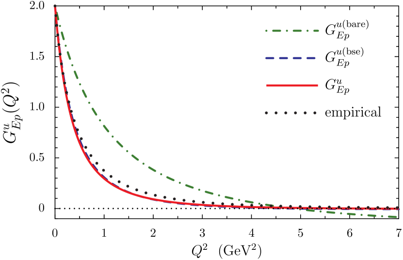
(a)

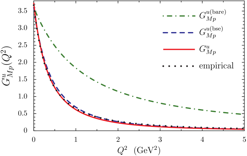
(b)

Figure 33: (Colour online) Proton up quark sector Sachs form factors. The empirical results are obtained using Ref. Kelly:2004hm and Eq. (47).

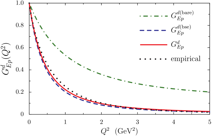
(a)

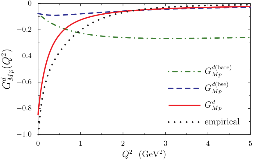
(b)

Figure 34: (Colour online) Neutron up quark sector Sachs form factors. The empirical results are obtained using Ref. Kelly:2004hm and Eq. (47).

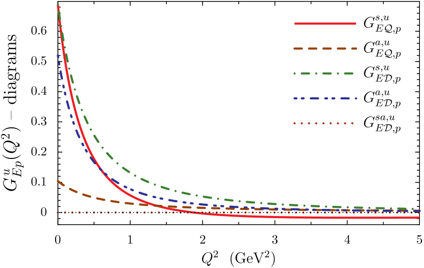
(a)

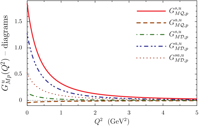
(b)

Figure 35: (Colour online) Total contributions to the proton $u$-sector Sachs form factors from each Feynman diagram in Fig. 4. These results include both the vector and tensor coupling contributions and the sum gives the total $u$-sector Sachs proton form factors.

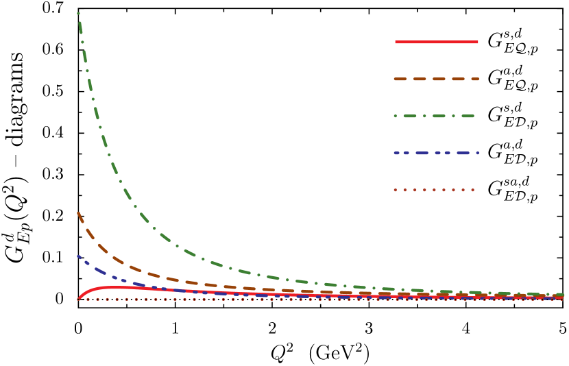
(a)

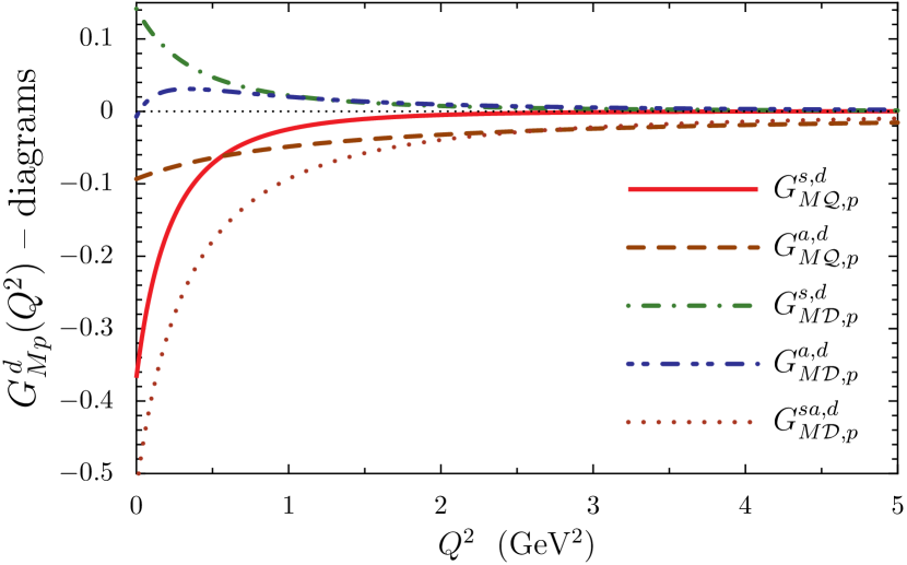
(b)

Figure 36: (Colour online) Total contributions to the neutron $u$-sector Sachs form factors from each Feynman diagram in Fig. 4. These results include both the vector and tensor coupling contributions and the sum gives the total $u$-sector Sachs neutron form factors.

Our results for the proton and neutron Sachs form factors are presented in Figs. 22 and 23, where in each case we have used the three variants of dressed quark form factor discussed in Sect. IV. Empirical results from Ref. Kelly:2004hm are shown as the dotted line. After including the vertex dressing from the BSE and also pion loop effects, the agreement with experiment is good. The proton electric form factor is slightly too soft and, as already discussed, possess a zero at $Q^{2}\simeq 3.7\,$GeV². For the proton magnetic form factor there is excellent agreement with the empirical results of Ref. Kelly:2004hm . Our result for the neutron electric form factor drops too slowly for $Q^{2}\gtrsim 1\,$GeV² and the magnetic form factor lacks a little strength for $Q^{2}\lesssim 1\,$GeV². However, overall the agreement with data is very good.

Results for the the proton quark sector Sachs form factors are given in Figs. 33 for the $u$-quark sector and Figs. 34 for the $d$-quark sector. Empirical results are obtained from Ref. Kelly:2004hm using the identities

$$G^{u}_{ip} =2\,G_{ip}+G_{in}, G^{d}_{ip} =G_{ip}+2\,G_{in},$$ (153)

where $i=(E,\,M)$. Overall the agreement with experiment is very good. Interestingly however, is that the pion loop effects have little influence on the quark sector Sachs form factors with the notable exception of $G_{Mp}^{d}(Q^{2})$. Here the pion cloud results in a 10-fold increase in the magnitude of the $d$ quark sector magnetic moment, from $\mu_{d}^{\text{(bse)}}=-0.075\,\mu_{N}$ to $\mu_{d}=-0.85\,\mu_{N}$. There are a number of effects that all add to give this very large pion loop correction, most importantly however, is the large $d$ quark sector anomalous magnetic moment of a dressed up quark (Eq. (82)) generated by the pion cloud. This results in a large contribution to $G_{Mp}^{d}(Q^{2})$ from the quark diagram where the photon couples to a dressed up quark, with a scalar diquark as spectator. Another notable result is that the zero in $G_{Ep}(Q^{2})$ resides solely in the $u$ quark sector, as illustrated by the upper panels of Figs. 33 and 34.

To understand these results better in we give the total contribution from each diagram, including both the BSE vertex dressing and pion loop effects in Figs. 35 for the $u$ quark sector and Figs. 36 for the $d$ quark sector. For the upper panel in Figs. 35 it is clear that the zero in $G_{Ep}^{u}(Q^{2})$ and therefore $G_{Ep}(Q^{2})$ has its origin solely in $G_{E\mathcal{Q},p}^{s,u}$, the $u$ quark sector contribution from quark diagrams with a spectator scalar diquark. We also find the interesting result that the diagrams associated with transitions between scalar and axialvector diquarks are identically zero for the Sachs electric form factors but do contribute sizeably to the Sachs magnetic form factors.

Appendix D Analysis of Pion Cloud effects

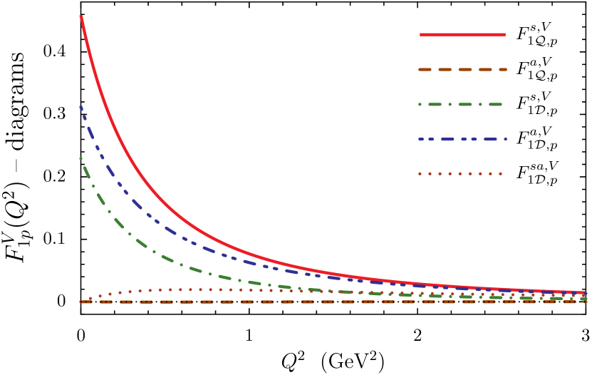
(a)

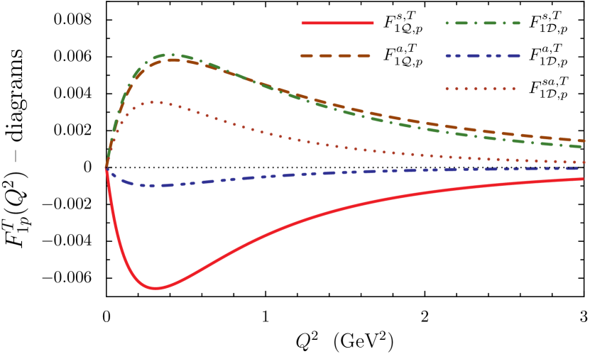
(b)

Figure 37: (Colour online) Total contributions to the proton Dirac form factor from each Feynman diagram in Fig. 4 for a vector coupling (upper panel) and tensor coupling (lower panel) to the dressed quarks. The sum of these 10 contributions gives the total proton Dirac form factor illustrated in Fig. 20 (solid curve).

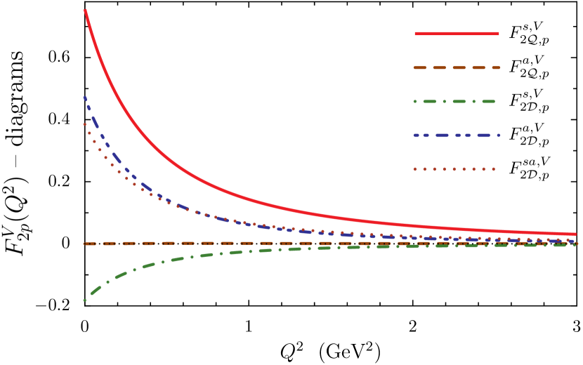
(a)

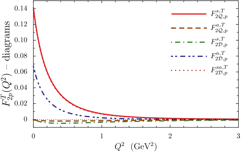
(b)

Figure 38: (Colour online) Total contributions to the proton Pauli form factor from each Feynman diagram in Fig. 4 for a vector coupling (upper panel) and tensor coupling (lower panel) to the dressed quarks. The sum of these 10 contributions gives the total proton Pauli form factor illustrated in Fig. 20 (solid curve).

A deeper understanding of our results is gained by decomposing the form factors in Figs. 20 and 21 into the various total contributions arising from each of the six diagrams represented in Fig. 4, for both the vector and tensor coupling to the dressed quarks. In this case the nucleon form factors are expressed as

$$F_{ip}(Q^{2})=F^{V}_{ip}(Q^{2})+F^{T}_{ip}(Q^{2}),$$ (154)

$$F_{in}(Q^{2})=F^{V}_{in}(Q^{2})+F^{T}_{in}(Q^{2}),$$ (155)

where $i=(1,\,2)$. In terms of the six diagrams contained in Fig. 4 we have

$$F^{V}_{ip} =F^{s,V}_{i\mathcal{Q},p}+F^{a,V}_{i\mathcal{Q},p}+F^{s,V}_{i\mathcal{D},p}+F^{a,V}_{i\mathcal{D},p}+F^{sa,V}_{i\mathcal{D},p},$$ (156)

$$F^{T}_{ip} =F^{s,T}_{i\mathcal{Q},p}+F^{a,T}_{i\mathcal{Q},p}+F^{s,T}_{i\mathcal{D},p}+F^{a,T}_{i\mathcal{D},p}+F^{sa,T}_{i\mathcal{D},p},$$ (157)

and neutron expressions are obtained by $p\to n$. All terms in Eqs. (156) and (157) include the isospin coefficients and the dressed quark form factors.

	$F^{s,V}_{1\mathcal{Q}}$	$F^{a,V}_{1\mathcal{Q}}$	$F^{s,V}_{1\mathcal{D}}$	$F^{a,V}_{1\mathcal{D}}$	$F^{sa,V}_{1\mathcal{D}}$	$F^{s,T}_{1\mathcal{Q}}$	$F^{a,T}_{1\mathcal{Q}}$	$F^{s,T}_{1\mathcal{D}}$	$F^{a,T}_{1\mathcal{D}}$	$F^{sa,T}_{1\mathcal{D}}$	total
$F_{1p}$	-0.46	0	-0.23	-0.31	0	0	0	0	0	0	-1
$F_{2p}$	-0.76	0	-0.18	-0.47	0.38	-0.14	0.0	0.0	-0.07	0.14	-1.78
$F_{1n}$	-0.23	-0.10	-0.23	-0.10	0	0	0	0	0	0	-0
$F_{2n}$	-0.38	-0.15	-0.18	-0.16	-0.38	-0.25	0.0	0.0	-0.17	-0.14	-1.81

Table 10: Total contributions to the nucleon Dirac and Pauli form factors from the various diagrams at $Q^{2}=0$. The vector contributions are obtained from the appropriate body form factors at $Q^{2}=0$ multiplied by isospin factors and quark charges. Therefore, the vector results do not change with the various approximations for the dressed quark form factors. The tensor contributions are only non-zero if the dressed quarks have an anomalous magnetic moment, and in this framework this occurs solely from pion loop effects. Rows with an entry of “0” are identically zero because of charge conservation.

Figs. 37 and 38 illustrate the results for the total contributions from each diagram in Fig. 4 to the proton form factors, where the contribution from the vector and tensor quark-photon couplings are shown separately. Results for the various contributions at $Q^{2}=0$ are also listed in rows 1 and 2 of Table 10. These results demonstrate the dominance of the scalar diquark component in the proton wave function. For example, diagrams which contain only a scalar diquark carry 69% of the proton charge and 40% of its anomalous magnetic moment, while diagrams that contain only axialvector diquarks carry 31% of the proton charge and 30% of its anomalous magnetic moment. The remainder of the anomalous magnetic moment, 30%, is carried by diagrams with both scalar and axialvector diquarks. The contributions that arise from the tensor coupling to the dressed quarks, illustrated in the lower panels of Figs. 37 and 38, diminish rapidly with increasing $Q^{2}$ because they are suppressed by the dressed quark Pauli form factors, illustrated in Fig. 6, which vanish monotonically for increasing $Q^{2}$.

The coupling of the photon to the diquarks is not only necessary for charge conservation, but is critical for a good description of the experimental data. Here the axialvector diquarks play an important role. For a proton, the photon is twice as likely to couple to a $\{uu\}$ type axialvector diquark than one of type $\{ud\}$. Furthermore, axialvector diquarks of type $\{uu\}$ have a charge of $4/3$ and a magnetic moment of $3.27\,\mu_{N}$ (see Tab. 3) and hence they provide the second largest contribution to the proton charge and anomalous magnetic moment. The largest contribution in each case comes from the quark diagram with a spectator scalar diquark. With the exception of the diquark diagram with an axialvector diquark spectator, the Feynman diagrams of Fig. 4, for the vector coupling, can only contribute to $F_{2p}(Q^{2})$ if the quarks have non-zero orbital angular momentum. The sizeable contributions from all other diagrams (see Fig. 38) indicate that there is significant quark orbital angular momentum in the proton wave function Myhrer:2007cf ; Thomas:2008ga .

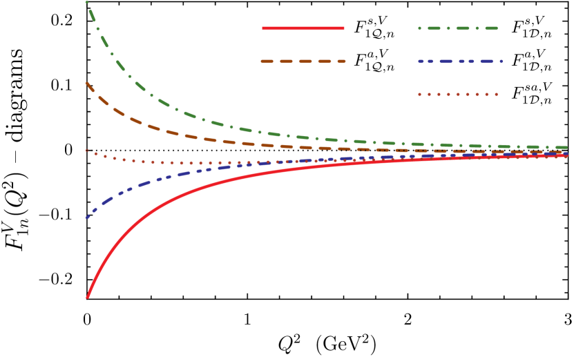
(a)

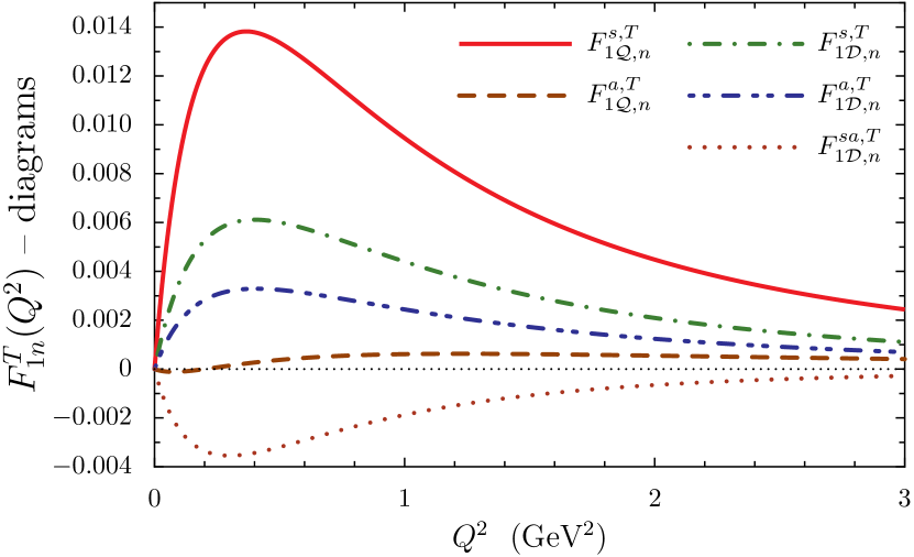
(b)

Figure 39: (Colour online) Total contributions to the neutron Dirac form factor from each Feynman diagram in Fig. 4 for a vector quark coupling (upper panel) and tensor quark coupling (lower panel). The sum of these 10 contributions gives the total neutron Dirac form factor illustrated in Fig. 21 (solid curve).

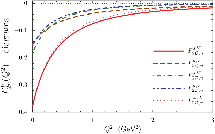
(a)

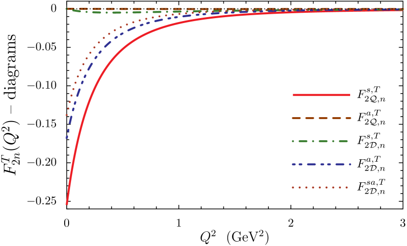
(b)

Figure 40: (Colour online) Total contributions to the neutron Pauli form factor from each Feynman diagram in Fig. 4 for a vector quark coupling (upper panel) and tensor quark coupling (lower panel). The sum of these 10 contributions gives the total neutron Dirac form factor illustrated in Fig. 21 (solid curve).

Figures 39 and 40 and rows 3 and 4 of Table 10 give results for the neutron form factors, broken down into the total vector and tensor coupling contributions from the Feynman diagrams of Fig. 4. For the Dirac form factor the diagram pairs with the same quark–diquark structure cancel each other to give a charge of zero, while diagrams that contain only scalar diquarks carry 45% of the neutron anomalous magnetic moment and diagrams containing only axialvector diquarks carry 27%. The remaining 28% is carried by diagrams with both scalar and axialvector diquarks. The tensor coupling contributions to $F_{1n}(Q^{2})$ are much more significant compared to the proton case, an indication of the particular sensitivity of the neutron Dirac form factor to pion cloud effects. axialvector diquarks play a reduced role in neutron structure, compared to the proton, because the $\{dd\}$ type axialvector diquark has half the charge and an anomalous magnetic moment 65% the size of the $\{uu\}$ type diquark found in the proton.

References

- (1) M. K. Jones et al. [Jefferson Lab Hall A Collaboration], Phys. Rev. Lett. 84, 1398 (2000) [nucl-ex/9910005].
- (2) O. Gayou et al. [Jefferson Lab Hall A Collaboration], Phys. Rev. Lett. 88, 092301 (2002) [nucl-ex/0111010].
- (3) O. Gayou, K. Wijesooriya, A. Afanasev, M. Amarian, K. Aniol, S. Becher, K. Benslama and L. Bimbot et al., Phys. Rev. C 64, 038202 (2001).
- (4) A. J. R. Puckett, E. J. Brash, M. K. Jones, W. Luo, M. Meziane, L. Pentchev, C. F. Perdrisat and V. Punjabi et al., Phys. Rev. Lett. 104, 242301 (2010) [arXiv:1005.3419 [nucl-ex]].
- (5) A. J. R. Puckett, E. J. Brash, O. Gayou, M. K. Jones, L. Pentchev, C. F. Perdrisat, V. Punjabi and K. A. Aniol et al., Phys. Rev. C 85, 045203 (2012) [arXiv:1102.5737 [nucl-ex]].
- (6) S. J. Brodsky and G. R. Farrar, Phys. Rev. Lett. 31, 1153 (1973).
- (7) S. J. Brodsky and G. R. Farrar, Phys. Rev. D 11, 1309 (1975).
- (8) J. P. Ralston and P. Jain, Phys. Rev. D 69, 053008 (2004) [hep-ph/0302043].
- (9) R. Pohl, A. Antognini, F. Nez, F. D. Amaro, F. Biraben, J. M. R. Cardoso, D. S. Covita and A. Dax et al., Nature 466, 213 (2010).
- (10) A. Antognini, F. Nez, K. Schuhmann, F. D. Amaro, FrancoisBiraben, J. M. R. Cardoso, D. S. Covita and A. Dax et al., Science 339, 417 (2013).
- (11) I. C. Cloët and G. A. Miller, Phys. Rev. C 83, 012201 (2011) [arXiv:1008.4345 [hep-ph]].
- (12) G. A. Miller, A. W. Thomas, J. D. Carroll and J. Rafelski, Phys. Rev. A 84, 020101 (2011) [arXiv:1101.4073 [physics.atom-ph]].
- (13) J. D. Carroll, A. W. Thomas, J. Rafelski and G. A. Miller, Phys. Rev. A 84, 012506 (2011) [arXiv:1104.2971 [physics.atom-ph]].
- (14) V. N. Gribov and L. N. Lipatov, Sov. J. Nucl. Phys. 15, 675 (1972) [Yad. Fiz. 15, 1218 (1972)].
- (15) G. Altarelli and G. Parisi, Nucl. Phys. B 126, 298 (1977).
- (16) Y. L. Dokshitzer, Sov. Phys. JETP 46, 641 (1977) [Zh. Eksp. Teor. Fiz. 73, 1216 (1977)].
- (17) Y. Nambu and G. Jona-Lasinio, Phys. Rev. 122, 345 (1961).
- (18) Y. Nambu and G. Jona-Lasinio, Phys. Rev. 124, 246 (1961).
- (19) U. Vogl and W. Weise, Prog. Part. Nucl. Phys. 27, 195 (1991).
- (20) T. Hatsuda and T. Kunihiro, Phys. Rept. 247, 221 (1994) [hep-ph/9401310].
- (21) S. P. Klevansky, Rev. Mod. Phys. 64, 649 (1992).
- (22) A. W. Thomas, S. Theberge and G. A. Miller, Phys. Rev. D 24, 216 (1981).
- (23) S. Theberge and A. W. Thomas, Nucl. Phys. A 393, 252 (1983).
- (24) A. W. Thomas, Adv. Nucl. Phys. 13, 1 (1984).
- (25) N. Ishii, W. Bentz and K. Yazaki, Phys. Lett. B 301, 165 (1993).
- (26) N. Ishii, W. Bentz and K. Yazaki, Phys. Lett. B 318, 26 (1993).
- (27) N. Ishii, W. Bentz and K. Yazaki, Nucl. Phys. A 587, 617 (1995).
- (28) H. Mineo, W. Bentz, N. Ishii, A. W. Thomas and K. Yazaki, Nucl. Phys. A 735, 482 (2004) [nucl-th/0312097].
- (29) I. C. Cloët, W. Bentz and A. W. Thomas, Phys. Rev. Lett. 95, 052302 (2005) [nucl-th/0504019].
- (30) I. C. Cloët, W. Bentz and A. W. Thomas, Phys. Lett. B 621, 246 (2005) [hep-ph/0504229].
- (31) I. C. Cloët, W. Bentz and A. W. Thomas, Phys. Lett. B 642, 210 (2006) [nucl-th/0605061].
- (32) I. C. Cloët, W. Bentz and A. W. Thomas, Phys. Lett. B 659, 214 (2008) [arXiv:0708.3246 [hep-ph]].
- (33) T. Ito, W. Bentz, I. C. Cloët, A. W. Thomas and K. Yazaki, Phys. Rev. D 80, 074008 (2009) [arXiv:0906.5362 [nucl-th]].
- (34) H. H. Matevosyan, A. W. Thomas and W. Bentz, Phys. Rev. D 83, 074003 (2011) [arXiv:1011.1052 [hep-ph]].
- (35) H. H. Matevosyan, W. Bentz, I. C. Cloët and A. W. Thomas, Phys. Rev. D 85, 014021 (2012) [arXiv:1111.1740 [hep-ph]].
- (36) H. H. Matevosyan, A. W. Thomas and W. Bentz, Phys. Rev. D 86, 034025 (2012) [arXiv:1205.5813 [hep-ph]].
- (37) W. Bentz and A. W. Thomas, Nucl. Phys. A 696, 138 (2001) [nucl-th/0105022].
- (38) M. Buballa, Phys. Rept. 407, 205 (2005) [hep-ph/0402234].
- (39) D. Ebert, T. Feldmann and H. Reinhardt, Phys. Lett. B 388, 154 (1996) [hep-ph/9608223].
- (40) G. Hellstern, R. Alkofer and H. Reinhardt, Nucl. Phys. A 625, 697 (1997) [hep-ph/9706551].
- (41) P. Maris and C. D. Roberts, Int. J. Mod. Phys. E 12, 297 (2003) [nucl-th/0301049].
- (42) H. L. L. Roberts, L. Chang, I. C. Cloët and C. D. Roberts, Few Body Syst. 51, 1 (2011) [arXiv:1101.4244 [nucl-th]].
- (43) F. E. Close and A. W. Thomas, Phys. Lett. B 212, 227 (1988).
- (44) A. W. Schreiber, P. J. Mulders, A. I. Signal and A. W. Thomas, Phys. Rev. D 45, 3069 (1992).
- (45) M. Hess, F. Karsch, E. Laermann and I. Wetzorke, Phys. Rev. D 58, 111502 (1998) [hep-lat/9804023].
- (46) A. Bender, C. D. Roberts and L. Von Smekal, Phys. Lett. B 380, 7 (1996) [nucl-th/9602012].
- (47) A. Buck, R. Alkofer and H. Reinhardt, Phys. Lett. B 286, 29 (1992).
- (48) H. Mineo, W. Bentz and K. Yazaki, Phys. Rev. C 60, 065201 (1999) [nucl-th/9907043].
- (49) H. Mineo, W. Bentz, N. Ishii and K. Yazaki, Nucl. Phys. A 703, 785 (2002) [nucl-th/0201082].
- (50) F. J. Ernst, R. G. Sachs and K. C. Wali, Phys. Rev. 119, 1105 (1960).
- (51) R. D. Young, J. Roche, R. D. Carlini and A. W. Thomas, Phys. Rev. Lett. 97, 102002 (2006) [nucl-ex/0604010].
- (52) K. A. Aniol et al. [HAPPEX Collaboration], Phys. Rev. Lett. 96, 022003 (2006) [nucl-ex/0506010].
- (53) D. S. Armstrong et al. [G0 Collaboration], Phys. Rev. Lett. 95, 092001 (2005) [nucl-ex/0506021].
- (54) S. Baunack, K. Aulenbacher, D. Balaguer Rios, L. Capozza, J. Diefenbach, B. Glaser, D. von Harrach and Y. Imai et al., Phys. Rev. Lett. 102, 151803 (2009) [arXiv:0903.2733 [nucl-ex]].
- (55) G. D. Cates, C. W. de Jager, S. Riordan and B. Wojtsekhowski, Phys. Rev. Lett. 106, 252003 (2011) [arXiv:1103.1808 [nucl-ex]].
- (56) P. Maris and P. C. Tandy, Phys. Rev. C 61, 045202 (2000) [nucl-th/9910033].
- (57) S. R. Amendolia et al. [NA7 Collaboration], Nucl. Phys. B 277, 168 (1986).
- (58) S. R. Amendolia, B. Badelek, G. Batignani, G. A. Beck, F. Bedeschi, E. H. Bellamy, E. Bertolucci and D. Bettoni et al., Phys. Lett. B 146, 116 (1984).
- (59) T. Horn et al. [Jefferson Lab F(pi)-2 Collaboration], Phys. Rev. Lett. 97, 192001 (2006) [nucl-ex/0607005].
- (60) V. Tadevosyan et al. [Jefferson Lab F(pi) Collaboration], Phys. Rev. C 75, 055205 (2007) [nucl-ex/0607007].
- (61) H. P. Blok et al. [Jefferson Lab Collaboration], Phys. Rev. C 78, 045202 (2008) [arXiv:0809.3161 [nucl-ex]].
- (62) G. P. Lepage and S. J. Brodsky, Phys. Lett. B 87, 359 (1979).
- (63) G. R. Farrar and D. R. Jackson, Phys. Rev. Lett. 43, 246 (1979).
- (64) M. Gluck, E. Reya and A. Vogt, Eur. Phys. J. C 5, 461 (1998) [hep-ph/9806404].
- (65) L. Chang, I. C. Cloët, C. D. Roberts, S. M. Schmidt and P. C. Tandy, Phys. Rev. Lett. 111, 141802 (2013) [arXiv:1307.0026 [nucl-th]].
- (66) E. B. Dally, J. M. Hauptman, J. Kubic, D. H. Stork, A. B. Watson, Z. Guzik, T. S. Nigmanov and V. D. Ryabtsov et al., Phys. Rev. Lett. 48, 375 (1982).
- (67) L. L. Frankfurt and M. I. Strikman, Nucl. Phys. B 148, 107 (1979).
- (68) S. J. Brodsky and J. R. Hiller, Phys. Rev. D 46, 2141 (1992).
- (69) J. J. Kelly, Phys. Rev. C 70, 068202 (2004).
- (70) J. Beringer et al. [Particle Data Group Collaboration], Phys. Rev. D 86, 010001 (2012).
- (71) X. Zhan, K. Allada, D. S. Armstrong, J. Arrington, W. Bertozzi, W. Boeglin, J. -P. Chen and K. Chirapatpimol et al., Phys. Lett. B 705, 59 (2011) [arXiv:1102.0318 [nucl-ex]].
- (72) J. C. Bernauer et al. [A1 Collaboration], Phys. Rev. Lett. 105, 242001 (2010) [arXiv:1007.5076 [nucl-ex]].
- (73) I. Sick, Prog. Part. Nucl. Phys. 67, 473 (2012).
- (74) I. C. Cloët, G. Eichmann, B. El-Bennich, T. Klahn and C. D. Roberts, Few Body Syst. 46, 1 (2009) [arXiv:0812.0416 [nucl-th]].
- (75) I. C. Cloët, C. D. Roberts and A. W. Thomas, Phys. Rev. Lett. 111, 101803 (2013) [arXiv:1304.0855 [nucl-th]].
- (76) S. Riordan, S. Abrahamyan, B. Craver, A. Kelleher, A. Kolarkar, J. Miller, G. D. Cates and N. Liyanage et al., Phys. Rev. Lett. 105, 262302 (2010) [arXiv:1008.1738 [nucl-ex]].
- (77) M. Diehl, Phys. Rept. 388, 41 (2003) [hep-ph/0307382].
- (78) A. V. Belitsky and A. V. Radyushkin, Phys. Rept. 418, 1 (2005) [hep-ph/0504030].
- (79) C. Itzykson and J. B. Zuber, New York, Usa: Mcgraw-hill (1980) 705 P.(International Series In Pure and Applied Physics)
- (80) F. Myhrer and A. W. Thomas, Phys. Lett. B 663, 302 (2008) [arXiv:0709.4067 [hep-ph]].
- (81) A. W. Thomas, Phys. Rev. Lett. 101, 102003 (2008) [arXiv:0803.2775 [hep-ph]].