[Critical Metrics]Critical Metrics for Riemannian Curvature Functionals

Introduction

The goal of these lectures is to gain an understanding of critical points of certain Riemmannian functionals. The starting point will be the (normalized) Einstein-Hilbert functional:

$$\tilde{\mathcal{E}}(g)=Vol(g)^{\frac{2-n}{n}}\int_{M}R_{g}dV_{g},$$

where $R_{g}$ is the scalar curvature. The Euler-Lagrange equations of $\tilde{\mathcal{E}}(g)$ are

(0.1) $$Ric(g)=\lambda\cdot g,$$

where $Ric$ denotes the Ricci tensor, and $\lambda$ is a constant. A Riemannian manifold $(M,g)$ satisfying (0.1) is called an Einstein manifold.

In Lecture Introduction, we will study the first and second variation of the functional $\tilde{\mathcal{E}}(g)$, and give an analysis of the Jacobi operator on transverse-traceless tensors. In Lecture 0.14, we will study conformal variations, discuss the Lichnerowicz eigenvalue estimate and Obata’s Theorem, and give a survey of the Yamabe Problem. In Lecture 0.25, we will introduce an important splitting of the space of symmetric $2$-tensors into pure-trace directions, transverse-traceless directions, and “diffeomorphism” directions. An infinitesimal version of the Ebin-Palais slice theorem will show that the diffeomorphism directions can be ignored. It will follow that critical points of the Einstein-Hilbert functional are in general saddle points. This leads one naturally to define the smooth Yamabe invariant of a manifold, or $\sigma$-constant.

Next, in Lecture 0.14.2, we will study the space of Einstein metrics modulo diffeomorphism, and use Fredholm theory to construct a map between finite-dimensional spaces called the Kuranishi map whose zero set is locally in one-to-one correspondence with the moduli space of Einstein metrics (locally). We will also discuss some basic rigidity results for Einstein metrics.

The topic in Lecture 0.51 will be quadratic curvature functionals in dimension four, that is linear combinations of the following quadratic curvature functionals:

$$\mathcal{W}(g)=\int_{M}|W_{g}|^{2}dV_{g},\ \ \rho(g)=\int_{M}|Ric_{g}|^{2}dV_{g},\ \ \mathcal{S}(g)=\int_{M}R_{g}^{2}dV_{g}.$$

Einstein metrics are critical for these functionals, and we will give a discussion of some known results about Einstein metrics. There are also many non-Einstein critical metrics for various linear combinations of these functionals. There is a special family of critical metrics for $\mathcal{W}$ known as anti-self-dual metrics. In Lecture 0.65, we will study the deformation theory of such metrics, and discuss local properties of the moduli space and existence of the Kuranishi map. We will also discuss several other interesting properties of anti-self-dual metrics.

In Lecture 0.76, we will discuss some rigidity and stability results regarding critical metrics for quadratic curvature functionals, which are joint work with Matt Gursky. As mentioned above, critical points of the Einstein-Hilbert functional in general have a saddle-point structure. However, critical points for certain quadratic functionals have a nicer local variational structure, see Theorem 0.77. Several rigidity results will also be discussed (which will be crucial in the final lecture).

In Lecture 0.89, we will study a special class of metrics called asymptotically locally Euclidean metrics (ALE), and present several hyperkähler examples. We will also discuss a result about non-collapsed limits of Einstein metrics: with certain geometric assumptions, a subsequence will converge to an orbifold Einstein metric. A natural question is whether one can reverse this process; that is, can one start with an orbifold Einstein metric, use Ricci-flat ALE metrics to resolve the singularities, and find an Einstein metric on the resolution? We will discuss a recent result of Biquard in the asymptotically hyperbolic Einstein setting which says that this is possible, provided that a certain obstruction vanishes.

We will next discuss a generalization of the Einstein condition, called $B^{t}$-flat metrics, give several examples, and discuss an analogous orbifold convergence result which is joint work with Gang Tian. In Lecture 0.37.1, we will present some of the key points of the proof of this result, and also give a discussion an Einstein metric on $\mathbb{CP}^{2}\#2\overline{\mathbb{CP}}^{2}$ found by Chen-LeBrun-Weber.

Finally, in Lecture 0.105 we will discuss an existence theorem for critical metrics on certain $4$-manifolds which is joint work with Matt Gursky. The general idea is to “glue” together two metrics which are critical for a functional to get an “approximate” critical metric, and then find conditions so that one can perturb to an actual solution. Theorem 0.107 produces critical metrics for specific functionals on the manifolds $\mathbb{CP}^{2}\#\overline{\mathbb{CP}}^{2},\mathbb{CP}^{2}\#2\overline{\mathbb{CP}}^{2}$, and $S^{2}\times S^{2}\#S^{2}\times S^{2}$.

This is an expanded version of lectures the author gave at the PCMI Program in Geometric Analysis in Park City from July 16-19, 2013.

The Einstein-Hilbert functional

0.1. Notation and conventions

The notation $\nabla_{X}Y$ will denote the covariant derivative on a Riemannian manifold $(M,g)$. In a coordinate system $\{x^{i}\}$, $i=1\dots n$, the Christoffel symbols are defined by

(0.2) $$\nabla_{\partial_{i}}\partial_{j}=\Gamma^{k}_{ij}\partial_{k},$$

where $\partial_{i}$ denotes the $i$th coordinate tangent vector field. The Christoffel symbols can be expressed in terms of the metric as

(0.3) $$\Gamma_{ij}^{k}=\frac{1}{2}g^{kl}\Big{(}\partial_{i}g_{jl}+\partial_{j}g_{il}-\partial_{l}g_{ij}\Big{)}.$$

The curvature tensor as a $(1,3)$-tensor is given by

(0.4) $$R(X,Y)Z=\nabla_{X}\nabla_{Y}Z-\nabla_{Y}\nabla_{X}Z-\nabla_{[X,Y]}Z,$$

and in coordinates our convention is

(0.5) $$R(\partial_{i},\partial_{j})\partial_{k}=R_{ijk}^{\ \ \ l}\partial_{l}.$$

The curvature tensor as a $(0,4)$-tensor is given by

(0.6) $$Rm(X,Y,Z,W)\equiv-g\big{(}R(X,Y)Z,W\big{)},$$

and in coordinates

(0.7) $$R_{ijkl}=Rm(\partial_{i},\partial_{j},\partial_{k},\partial_{l}).$$

Note that our convention is

(0.8) $$R_{ijlk}=R_{ijk}^{\ \ \ m}g_{ml}.$$

That is, we lower the upper index to the third position (warning: some authors to lower this index to a different position). The components of the Ricci tensor are given by

(0.9) $$R_{ij}=R_{lij}^{\ \ \ l}=g^{lm}R_{limj}=R_{ji},$$

and the scalar curvature is

(0.10) $$R=g^{pq}R_{pq}=g^{pq}g^{lm}R_{lpmq}.$$

0.2. First variation

We let $\mathcal{M}$ denote the space of Riemannian metrics on a manifold $M$:

(0.11) $$\mathcal{M}=\{g\in\Gamma(S^{2}(T^{*}M)),\ g\mbox{ is positive definite}\},$$

where $\Gamma(S^{2}(T^{*}M))$ denotes the space of smooth symmetric covariant $2$-tensors on $M$. The (unnormalized) Einstein-Hilbert functional $\mathcal{E}:\mathcal{M}\rightarrow\mathbb{R}$ is defined by

(0.12) $$\mathcal{E}(g)=\int_{M}R_{g}dV_{g}.$$

This is a Riemannian functional in the sense that it is invariant under diffeomorphisms:

(0.13) $$\mathcal{E}(\varphi^{*}g)=\mathcal{E}(g).$$

Next, we compute the Euler-Lagrange equations of the unnormalized functional:

Proposition 0.1.

If $M$ is closed and $n\geq 3$, then a metric $g\in\mathcal{M}$ is critical for $\mathcal{E}$ if and only if $g$ is Ricci-flat.

Proof.

Let $g(t)$ be a variation, with $h=g^{\prime}(0)$. Then

(0.14) $$\begin{split}\mathcal{E}(g(t))^{\prime}&=\int_{M}(R_{g(t)}dV_{g(t)})^{\prime}\\ &=\int_{M}R_{g(t)}^{\prime}dV_{g(t)}+R_{g(t)}(dV_{g(t)})^{\prime}\end{split}$$

Recall the formula for the linearization of the scalar curvature

(0.15) $$(R_{g(t)})^{\prime}\big{|}_{t=0} =-\Delta(trh)+\delta^{2}h-R_{lp}h^{lp},$$

where $\delta^{2}$ is the double-divergence operator defined in coordinates by

(0.16) $$\delta^{2}h=\nabla^{i}\nabla^{j}h_{ij},$$

and $\Delta$ is the Laplacian on functions (note that we use the analysts’ Laplacian, which has negative eigenvalues). We also recall the formula for the linearization of the volume element

(0.17) $$(dV_{g(t)})^{\prime}\big{|}_{t=0} =\frac{1}{2}tr_{g}(h)dV_{g}.$$

Next, we evaluate (0.14) at $t=0$, and consider $\mathcal{E}_{g}^{\prime}$ as a mapping on symmetric tensors. Substituting the formulas (0.15) and (0.17) into (0.14), and integrating by parts, we obtain

$$\mathcal{E}_{g}^{\prime}(h) =\int_{M}\Big{(}R^{\prime}+\frac{R}{2}tr_{g}(h)\Big{)}dV_{g}$$

$$=\int_{M}\Big{(}-\Delta(trh)+\delta^{2}h-R^{lp}h_{lp}+\frac{R}{2}tr_{g}(h)\Big{)}dV_{g}$$

$$=\int_{M}\Big{(}(-R^{lp}+\frac{R}{2}g^{lp})h_{lp}\Big{)}dV_{g}.$$

If this vanishes for all variations $h$, then

$$Ric=\frac{R}{2}g.$$

If $n>2$, taking a trace, we find that $R=0$, so $(M,g)$ is Ricci-flat. ∎

Remark 0.2.

If $n=2$ then $\mathcal{E}$ has zero variation, thus is constant. This is not surprising in view of the Gauss-Bonnet Theorem:

(0.18) $$\int_{M^{2}}K_{g}dV_{g}=2\pi\chi(M^{2}),$$

where $K_{g}=R_{g}/2$ is the Gaussian curvature, and $\chi$ denotes the Euler characteristic.

Exercise 0.3.

(i) Prove (0.15). (Hint: first prove that (0.3) linearizes to

(0.19) $$(\Gamma_{ij}^{k})^{\prime}=\frac{1}{2}g^{kl}\Big{(}\nabla_{i}h_{jl}+\nabla_{j}h_{il}-\nabla_{l}h_{ij}\Big{)}.$$

Next, write out a formula for the scalar curvature in terms of Christoffel symbols, and use (0.19). Note: these computations are much simpler if one works in a normal coordinate system, since the Christoffel symbols vanish at the base point in normal coordinates.)

(ii) Prove (0.17) using that the volume element is locally $dV_{g}=\sqrt{\det(g_{ij})}\cdot dx$.

0.2.1. Diffeomorphism invariance $\Rightarrow$ Bianchi identity

Define the divergence operator $\delta:\Gamma(S^{2}(T^{*}M))\rightarrow\Gamma(T^{*}M)$ by

(0.20) $$(\delta h)_{j}=g^{pq}\nabla_{p}h_{qj}.$$

The tensor that arises in the above calculation

(0.21) $$G=-Ric+\frac{R}{2}g,$$

is known as the Einstein tensor. By the contracted second Bianchi identity, it is divergence-free. This is actually a consequence of diffeomorphism invariance of the functional. To see this, let $\phi_{t}$ be a path of diffeomorphisms, and let $g_{t}=\phi_{t}^{*}g$. Then $g^{\prime}=\mathcal{L}_{X}g$, where $X$ is the tangent vector field of this $1$-parameter group of diffeomorphisms at $t=0$, and $\mathcal{L}$ is the Lie derivative operator. Integrating by parts:

$$\int_{M}\langle G,\mathcal{L}_{X}g\rangle dV_{g}=-\int_{M}\langle 2\delta G,X\rangle dV_{g},$$

for any vector field $X$, which implies that $\delta G=0$. Moreover, this argument shows that if $\mathcal{F}$ is any Riemannian functional, then $\delta\nabla\mathcal{F}=0$.

0.3. Normalized functional

The functional $\mathcal{E}$ is not scale-invariant for $n\geq 3$. To account for this, we define the normalized Einstein-Hilbert functional by

(0.22) $$\tilde{\mathcal{E}}(g)=Vol(g)^{\frac{2-n}{n}}\int_{M}R_{g}dV_{g}.$$

Proposition 0.4.

A metric $g$ is critical for $\tilde{\mathcal{E}}$ under all conformal variations (those of the form $h=f\cdot g$ for $f:M\rightarrow\mathbb{R}$) if and only if $g$ has constant scalar curvature. Furthermore, a metric $g\in\mathcal{M}$ is critical for $\tilde{\mathcal{E}}$ if and only if $g$ is Einstein, that is, $Ric(g)=\lambda\cdot g$ for some constant $\lambda\in\mathbb{R}$.

Proof.

We compute

$$\tilde{\mathcal{E}}^{\prime}(h) =Vol(g)^{\frac{2-n}{n}}\Big{(}\frac{2-n}{n}Vol(g)^{-1}\int_{M}\frac{1}{2}(tr_{g}h)dV_{g}\cdot\int_{M}R_{g}dV_{g}\Big{)}$$

$$\ \ \ \ \ +Vol(g)^{\frac{2-n}{n}}\int_{M}\Big{(}-R^{lp}+\frac{R}{2}g^{lp}\Big{)}h_{lp}dV_{g}.$$

If $g(t)=f(t)g$, then

$$\tilde{\mathcal{E}}^{\prime}(h)=\frac{n-2}{2n}Vol(g)^{\frac{2-n}{n}}\Big{(}\int_{M}(tr_{g}h)(R_{g}-\overline{R})dV_{g}\Big{)},$$

where $\overline{R}$ denotes the average scalar curvature. If this is zero for an arbitrary function $tr_{g}h$, then $R_{g}$ must be constant. The full variation then simplifies to

(0.23) $$\tilde{\mathcal{E}}^{\prime}(h)=Vol(g)^{\frac{2-n}{n}}\int_{M}\Big{(}-R^{lp}+\frac{R}{n}g^{lp}\Big{)}h_{lp}dV_{g}.$$

If this vanishes for all variations, then the traceless Ricci tensor must vanish, so $(M,g)$ is Einstein. ∎

0.4. Second variation

Since the functional is scale invariant, from now on we will always restrict to variations satisfying

(0.24) $$\int_{M}tr_{g}(h)dV_{g}=0.$$

Proposition 0.5.

Let $g$ be Einstein with $Ric(g)=\lambda\cdot g$. Then the second derivative of $\tilde{\mathcal{E}}$ at $t=0$ is given by

(0.25) $$\tilde{\mathcal{E}}^{\prime\prime}=Vol(g)^{\frac{2-n}{n}}\Big{\{}\frac{2-n}{2}\lambda\int_{M}|h|^{2}dV_{g}+\int_{M}\langle G^{\prime}(h),h\rangle dV_{g}\Big{\}}.$$

Proof.

The proof is left as an exercise. An important point is that the second derivative of a functional is well-defined at a critical point (it only depends on the tangent to the variation). ∎

Exercise 0.6.

Prove the formula for the linearization of the Ricci tensor,

(0.26) $$\begin{split}(Ric^{\prime})_{ij}&=\frac{1}{2}\Big{(}-\Delta h_{ij}+\nabla_{i}(\delta h)_{j}+\nabla_{j}(\delta h)_{i}-\nabla_{i}\nabla_{j}(tr_{g}h)\\ &\ \ \ \ \ \ \ -2R_{iljp}h^{lp}+R_{i}^{p}h_{jp}+R_{j}^{p}h_{ip}\Big{)},\end{split}$$

where $\Delta:\Gamma(S^{2}(T^{*}M))\rightarrow\Gamma(S^{2}(T^{*}M))$ is the rough Laplacian defined by

(0.27) $$(\Delta h)_{ij}=g^{pq}\nabla_{p}\nabla_{q}h_{ij}.$$

(Hint: write out a formula for the Ricci tensor in terms of Christoffel symbols, and use (0.19). Use normal coordinates to simplify the computation.)

Next, letting

(0.28) $$(Rm*h)_{ij}=R_{iljp}h^{lp},$$

equation (0.25) can be rewritten as follows.

Proposition 0.7.

Let $g$ be Einstein with $Ric(g)=\lambda\cdot g$. Then the second derivative of $\tilde{\mathcal{E}}$ at $t=0$ is given by

(0.29) $$\tilde{\mathcal{E}}^{\prime\prime}=Vol(g)^{\frac{2-n}{n}}\int_{M}\langle h,Jh\rangle dV_{g},$$

where $J:\Gamma(S^{2}(T^{*}M))\rightarrow\Gamma(S^{2}(T^{*}M))$ is the operator

(0.30) $$Jh=\frac{1}{2}\Delta h-\frac{1}{2}\mathcal{L}(\delta h)+(\delta^{2}h)g-\frac{1}{2}(\Delta tr_{g}h)g-\frac{\lambda}{2}(tr_{g}h)g+Rm*h.$$

0.5. Transverse-traceless variations

We next have the following definition.

Definition 0.8.

A symmetric $2$-tensor $h$ is called transverse-traceless (TT for short) if $\delta_{g}h=0$ and $tr_{g}(h)=0$.

The second variation formula simplifies considerably for TT variations:

Proposition 0.9.

If $h$ is transverse-traceless, then

(0.31) $$\tilde{\mathcal{E}}^{\prime\prime}=Vol(g)^{\frac{2-n}{n}}\Big{\{} \int_{M}\Big{\langle}h,\frac{1}{2}\Delta h+Rm*h\Big{\rangle}dV_{g}\Big{\}}.$$

The first term is manifestly negative, which shows that critical metrics for $\tilde{\mathcal{E}}$ always have a saddle point structure. In other words, modulo a finite dimensional space, $\tilde{\mathcal{E}}$ is locally strictly maximizing in TT directions.

0.5.1. The case of constant curvature

If $(M,g)$ has constant sectional curvature, then

(0.32) $$R_{ijkl}=k_{0}(g_{ik}g_{jl}-g_{jk}g_{il}).$$

The above second variation formula for TT tensors simplifies to

(0.33) $$\tilde{\mathcal{E}}^{\prime\prime}=Vol(g)^{\frac{2-n}{n}}\Big{\{} \int_{M}\Big{\langle}h,\frac{1}{2}\Delta h-k_{o}h\Big{\rangle}dV_{g}\Big{\}}.$$

This immediately yields:

Corollary 0.10.

Let $(M^{n},g)$ have constant sectional curvature $k_{0}$. If $k_{0}>0$ and $n>2$, then the second variation is strictly negative when restricted to transverse-traceless variations. If $k_{0}=0$, then the second variation is strictly negative except for parallel $h$.

For $n=2$, as pointed out above, we know that $\tilde{\mathcal{E}}$ is constant; thus our computation shows that if $h$ is TT then $h$ is identically zero on $S^{2}$, and $h$ must be parallel on $T^{2}$. The parallel sections in the case $k_{0}=0$ correspond to deformations of the flat structure, this will be discussed in more detail in Lecture 0.14.2 (also see Exercise 0.50 below).

0.5.2. Hyperbolic manifolds

In the hyperbolic case, we have

Lemma 0.11.

If $(M^{n},g)$ is compact and hyperbolic, then the smallest eigenvalue of the rough Laplacian on TT tensors is at least $n$.

Proof.

Exercise. Hint: start with the inequality

(0.34) $$\int_{M}|\nabla_{i}h_{jk}-\nabla_{j}h_{ik}|^{2}dV_{g}\geq 0,$$

integrate by parts, commute covariant derivatives, etc. ∎

This immediately yields

Corollary 0.12.

If $(M^{n},g)$ is hyperbolic and $n>2$, then $\tilde{\mathcal{E}}$ is locally strictly maximizing in TT directions.

Define the operator $d^{\nabla}:\Gamma(S^{2}_{0}(T^{*}M))\rightarrow\Gamma(\Lambda^{2}\otimes T^{*}M)$ by

(0.35) $$(d^{\nabla}h)_{ijk}=\nabla_{i}h_{jk}-\nabla_{j}h_{ik},$$

which is called the Codazzi operator. From the proof of Lemma 0.11, the eigentensors corresponding to the least eigenvalue of the rough Laplacian are exactly the Codazzi tensor, that is, $d^{\nabla}h=0$. These yield kernel elements of the second variation when $n=2$, this will be examined in more detail below in Lecture 0.14.2.

0.5.3. The case of $S^{2}\times S^{2}$

A nice example with saddle-point structure in the TT-directions is given by the product metric on $S^{2}\times S^{2}$. Let $\pi_{i}:S^{2}\times S^{2}\rightarrow S^{2}$ denote the projection onto the $i$th factor for $i=1,2$. The product metric is $g=g_{1}+g_{2}$ where $g_{i}=\pi_{i}^{*}g_{S^{2}}$, and $g_{S^{2}}$ is the round metric on $S^{2}$ of constant Gaussian curvature equal to $1$.

Proposition 0.13.

On $S^{2}\times S^{2}$ with the product metric $g_{1}+g_{2}$, the lowest eigenvalue of the operator $\frac{1}{2}\Delta h+Rm*h$ on TT tensors is $-1$. The corresponding eigenspace is $1$-dimensional, and is spanned by $h=g_{1}-g_{2}$. The next largest eigenvalue is $1$.

Proof.

This is left as an exercise, with the following hint: decompose a traceless symmetric $2$-tensor as

(0.36) $$h=\overset{\circ}{h_{1}}+\frac{f}{m}g_{1}+\hat{h}+\overset{\circ}{h_{2}}-\frac{f}{m}g_{2},$$

where $h_{i}$ is the pull-back of a tensor from the $i$th factor, $\overset{\circ}{h_{i}}$ is its trace-free part, for $i=1,2$, and $\hat{h}$ are the mixed directions. Since the curvature tensor is given by

(0.37) $$R_{ijkl}=(g_{1})_{ik}(g_{1})_{jl}-(g_{1})_{jk}(g_{1})_{il}+(g_{2})_{ik}(g_{2})_{jl}-(g_{2})_{jk}(g_{2})_{il},$$

the eigenvalue equation reduces to three separate equations on the pieces in the decomposition (0.36), which can be analyzed separately. For more details, see for example [GV11, Proposition 7.9]. ∎

Exercise 0.14.

(i) Find a constant scalar curvature deformation of the product metric corresponding to $h=g_{1}-g_{2}$, and which increases the functional $\tilde{\mathcal{E}}$.

(ii) Show that $\alpha_{1}\odot\alpha_{2}$ ($\odot$ = symmetric product), where $\alpha_{i}$ are $1$-forms dual to Killing fields are eigentensors with eigenvalue $1$.

Conformal geometry

0.6. Conformal variations

We will next look at conformal variations, that is, those variations of the form $h=f\cdot g$, for a function $f:M\rightarrow\mathbb{R}$.

Proposition 0.15.

Assume that $g$ has constant scalar curvature, and let $h=fg$ with $\int_{M}fdV_{g}=0$. Then

(0.38) $$\tilde{\mathcal{E}}^{\prime\prime}=Vol(g)^{\frac{2-n}{n}}\frac{2-n}{2}\Big{\{} \int_{M}\Big{(}(n-1)\Delta f+R_{g}f\Big{)}fdV_{g}\Big{\}}.$$

Proof.

Assuming $g$ is Einstein, this follows from the above formulas, but it is easy to verify that this holds more generally for constant scalar curvature metrics, the calculation is left as an exercise. ∎

Let $(S^{n},g_{S})$ denote the unit $n$-sphere with round metric $g_{S}$. Note that the Ricci tensor satisfies $Ric(g_{S})=(n-1)g_{S}$. An immediate corollary is the following

Corollary 0.16.

Let $g$ have constant scalar curvature. If $R_{g}\leq 0$ , then $\tilde{\mathcal{E}}$ is locally strictly minimizing in the conformal direction. If $R_{g}>0$ and $Ric\geq(n-1)g$, then the same is true, unless $g$ is isometric to $(S^{n},g_{S})$.

The case $R_{g}\leq 0$ is obvious and the case $R_{g}>0$ will follow from a result due to Lichnerowicz which we will discuss next. Let $\lambda_{1}$ denote the lowest non-trivial eigenvalue of the Laplacian on functions, that is $\Delta u=-\lambda_{1}u$. We have the following eigenvalue estimate which was proved by Lichnerowicz in 1958 in [Lic58], and for which the equality case was characterized by Obata in 1962 [Oba62]:

Theorem 0.17 (Lichnerowicz-Obata).

If a compact manifold $(M^{n},g)$ satisfies

(0.39) $$Ric\geq(n-1)\cdot g,$$

then $\lambda_{1}\geq n$, with equality if and only if $(M^{n},g)$ is isometric to $(S^{n},g_{S})$.

Proof.

We only give an outline of the proof. First, commuting covariant derivatives, write

(0.40) $$\int_{M}(\Delta f)^{2}dV_{g}=\int_{M}|\nabla^{2}f|^{2}dV_{g}+\int_{M}Ric(\nabla f,\nabla f)dV_{g},$$

and then use the matrix inequality $|A|^{2}\geq(1/n)(tr(A))^{2}$. If $\lambda_{1}=n$, then equality in this inequality implies that there is a non-trivial solution of the equation

(0.41) $$\nabla^{2}f=\frac{\Delta f}{n}g=-f\cdot g.$$

This implies that along any unit-speed geodesic,

(0.42) $$f(s)=A\cos(s)+B\sin(s),$$

where $s$ is the arc-length from a fixed point $P_{+}$. If we choose the point $P_{+}$ to be a maximum of $f$, then $f(s)=A\cos(s)$ along any geodesic through $P_{+}$. One then uses this information to construct an isometry with $(S^{n},g_{S})$. For more details, see [Oba62] and also [Küh88] for an excellent exposition. ∎

0.6.1. Conformal variations on $S^{n}$

On $(S^{n},g_{S})$, eigenfunctions corresponding to the eigenvalue $n$ yield directions with $\tilde{\mathcal{E}}^{\prime\prime}=0$. There is a nice geometric explanation for this fact:

Proposition 0.18.

Let $\phi_{t}$ be a $1$-parameter group of conformal automorphisms of $g_{S}$. Then

(0.43) $$\frac{d}{dt}(\phi_{t}^{*}g_{S})|_{t=0}=fg,$$

where $f$ is an eigenfunction satisfying $\Delta f=-nf$.

Proof.

We leave this as an exercise, with the following hint: use the Hodge decomposition to write any $1$-form $\alpha$ dual to a conformal vector field as $\alpha=df+\omega$, with $\omega$ divergence free. Apply the conformal Killing operator to $\alpha$ and use the resulting equation to show that the trace-free Hessian of $f$ vanishes, and that $\omega$ is Killing. ∎

0.7. Global conformal minimization

Actually, it turns out that something much stronger is true for Einstein metrics:

Theorem 0.19.

An Einstein metric $(M^{n},g)$ is the unique global minimizer of $\tilde{\mathcal{E}}$ in its conformal class (up to scaling), unless $(M,g)$ is isometric to $(S^{n},g_{S})$. In this case, any critical point is the pull-back of $g_{S}$ under a conformal diffeomorphism.

This will be proved below. The first key point in the proof is the following theorem of Obata:

Theorem 0.20 ([Oba72]).

If $(M^{n},g)$ is Einstein, then $g$ is the unique constant scalar curvature metric in its conformal class (up to scaling), unless $(M,g)$ is isometric to $(S^{n},g_{S})$, in which case all critical points are the pull-back of $g_{S}$ under a conformal diffeomorphism.

Proof.

To prove this, assume that $\hat{g}$ is a constant scalar curvature metric which is conformal to $g$. Letting $E$ denote the traceless Ricci tensor, we recall the transformation formula: if $g=\phi^{-2}\hat{g}$, then

(0.44) $$E_{g}=E_{\hat{g}}+(n-2)\phi^{-1}\big{(}\nabla^{2}\phi-(\Delta\phi/n)\hat{g}\big{)},$$

where $n$ is the dimension, and the covariant derivatives are taken with respect to $\hat{g}$. Since $g$ is Einstein, we have

(0.45) $$E_{\hat{g}}=(2-n)\phi^{-1}\big{(}\nabla^{2}\phi-\frac{1}{n}(\Delta\phi)\hat{g}\big{)}.$$

Integrating,

$$\int_{M}\phi|E_{\hat{g}}|^{2}dV_{\hat{g}} =(2-n)\int_{M}\phi E_{\hat{g}}^{ij}\left\{\phi^{-1}\big{(}\nabla^{2}\phi-\frac{1}{n}(\Delta\phi)\hat{g}\big{)}_{ij}\right\}dV_{\hat{g}}$$

$$=(2-n)\int_{M}E_{\hat{g}}^{ij}\nabla^{2}\phi_{ij}dV_{\hat{g}}$$

$$=(n-2)\int_{M}(\nabla_{j}E_{\hat{g}}^{ij}\cdot\nabla_{i}\phi)dV_{\hat{g}}=0,$$

by the Bianchi identity. Consequently, $\hat{g}$ is also Einstein. If $\hat{g}$ is not a constant multiple of $g$, then $(M,g)$ admits a nonconstant solution of the equation

(0.46) $$\nabla^{2}\phi=\frac{\Delta\phi}{n}g.$$

Taking a divergence of this equation, it follows that $\phi+c$, where $c$ is a constant, is an eigenfunction of the Laplacian with eigenvalue $n$, so $(M,g)$ is isometric to $(S^{n},g_{S})$ by the same argument in Theorem 0.17 given above. ∎

We will next take a slight detour and discuss the Yamabe Problem, before returning to the proof of Theorem 0.19.

0.8. Green’s function metric and mass

A key idea in the final resolution of the Yamabe Problem is the following construction of an asymptotically flat metric, called the Green’s function metric. First, we define an asymptotically flat metric:

Definition 0.21.

A complete Riemannian manifold $(X^{n},g)$ is called asymptotically flat or AF of order $\tau$ if there exists a diffeomorphism $\psi:X\setminus K\rightarrow(\mathbb{R}^{n}\setminus B(0,R))$ where $K$ is a compact subset of $X$, and such that under this identification,

(0.47) $$(\psi_{*}g)_{ij} =\delta_{ij}+O(\rho^{-\tau}),$$

(0.48) $$\ \partial^{|k|}(\psi_{*}g)_{ij} =O(\rho^{-\tau-k}),$$

for any partial derivative of order $k$, as $r\rightarrow\infty$, where $\rho$ is the distance to some fixed basepoint.

The conformal Laplacian is the operator:

(0.49) $$\square u=-4\frac{n-1}{n-2}\Delta u+Ru.$$

If $(M,g)$ is compact and $R>0$, then for any $p\in M$, there is a unique positive solution to the equation

(0.50) $$\begin{split}\square G&=0\ \ \mathrm{on}\ M\setminus\{p\}\\ G&=\rho^{2-n}(1+o(1))\end{split}$$

as $\rho\rightarrow 0$, where $\rho$ is geodesic distance to the basepoint $p$. This function $G$ is called the Green’s function for the conformal Laplacian.

Exercise 0.22.

Show that if $\tilde{g}=u^{\frac{4}{n-2}}g$, then

(0.51) $$\square_{g}u=R_{\tilde{g}}u^{\frac{n+2}{n-2}}.$$

Denote $N=M\setminus\{p\}$ with metric $g_{N}=G^{\frac{4}{n-2}}g_{M}$. From Exercise 0.22, $g_{N}$ is scalar-flat. From a more careful expansion of the Green’s function, it is possible to show that $g_{N}$ is also asymptotically flat, but we omit the proof.

The mass of an AF space is defined by

(0.52) $${\mathrm{mass}}(g_{N})=\lim_{R\rightarrow\infty}\frac{1}{\omega_{n-1}}\int_{S(R)}\sum_{i,j}(\partial_{i}g_{ij}-\partial_{j}g_{ii})(\partial_{i}\ \lrcorner\ dV_{g}),$$

where $\omega_{n-1}=Vol(S^{n-1})$, and $S(R)$ denotes the sphere of radius $R$. It was shown in [Bar86] that if $\tau>(n-2)/2$, then this mass is well-defined, that is, it is independent of the coordinate system chosen around infinity. The mass is consequently a geometric invariant of an AF metric, and plays an important rôle in the final resolution of the Yamabe Problem, which we discuss next.

0.9. The Yamabe Problem

By Hölder’s inequality, the functional $\tilde{\mathcal{E}}$ is bounded from below when restricted to any fixed conformal class. It is then natural to minimize in the conformal direction:

(0.53) $$Y(M,[g])=\inf_{\tilde{g}\in[g]}\tilde{\mathcal{E}}(\tilde{g}).$$

This is called the conformal Yamabe invariant.

Theorem 0.23.

If $(M^{n},g)$ is compact, then there exists a conformal metric $\tilde{g}\in[g]$ which has constant scalar curvature, and which minimizes $\tilde{\mathcal{E}}$ in its conformal class.

Outline of Proof..

For any conformal class, Aubin showed that

(0.54) $$Y(M,[g])\leq\tilde{\mathcal{E}}(g_{S}).$$

The idea of the proof of this estimate is to choose a conformal factor which is spherical in an $\epsilon$-neighborhood of a point, and zero everywhere else (this is called a “bubble”). Expanding the Yamabe energy of this test function in the parameter $\epsilon$ then yields a leading term which is exactly the Yamabe energy of the spherical metric.

Next, one shows that if this inequality is strict, then a solution exists. This step is now considered “trivial” by experts, but in fact this took a long time to figure out. Yamabe’s original paper [Yam60] contains a serious mistake on this point, this was fixed by Trudinger [Tru68], and then optimized by Aubin [Aub76].

The more difficult step is to show that if $(M,[g])$ is not conformally diffeomorphic to $(S^{n},[g_{S}])$ then the inequality (0.54) is strict. In case $n\geq 6$ and $g$ is not locally conformally flat, this was proved by Aubin [Aub76, Aub98] by basing the above test function at a point where the Weyl tensor does not vanish. The locally conformally flat case was proved by Schoen-Yau [SY88] using ideas involving the developing map. The case $n\leq 6$ was proved by Schoen [Sch84]. The main idea is the following. Instead of making the above test function be zero away from the bubble, Schoen’s idea was to instead choose the conformal factor to be the Green’s function for the conformal Laplacian away from the bubble. The mass of the associated asympotically flat metric arises as the next term in the expansion of the Yamabe energy of this test function, so the result follows from the positive mass theorem of Schoen-Yau [SY79, SY81, Sch89]. ∎

We next return to the global minimization statement in Theorem 0.19:

Proof of Theorem 0.19.

The uniqueness follows from Theorem 0.20. For the minimization statement, of course, we know a minimizer exists from the resolution of the Yamabe problem, but there is an “easy” proof in the Einstein case. In the negative or zero scalar curvature case, one can apply a standard argument from the calculus of variations to show that a minimizing sequence converges. In the positive case, scale so that $Ric=(n-1)g$. Then

(0.55) $$\tilde{\mathcal{E}}(g)=n(n-1)Vol(g)^{2/n}.$$

By Bishops’ volume comparison theorem, $Vol(M,g)\leq Vol(S^{n},g_{S})$ with equality if and only if $g$ is isometric to $g_{S}$. So if $g$ is not isometric to $g_{S}$, we have

(0.56) $$Y(M,[g])=\inf_{\tilde{g}\in[g]}\tilde{\mathcal{E}}(g)<\tilde{\mathcal{E}}(g_{S}).$$

As discussed above, this estimate implies that a minimizing sequence converges (no bubbles are possible).

Finally, the case of $(S^{n},g_{S})$ takes some extra work. One needs to suitably re-normalize a minimizing sequence using the conformal group to obtain a minimizing sequence which converges, see [LP87, Proposition 4.6] for an argument due to Karen Uhlenbeck.

∎

Remark 0.24.

An important question is if the set of unit volume constant scalar curvature metrics in a conformal class is compact if the manifold is not conformally diffeomorphic to the sphere. This is true in dimensions $n\leq 24$ [KMS09]. Surprisingly, it is false in higher dimensions [Bre08, BM09].

0.10. Generalizations of the Yamabe Problem

We mention that there are many other Yamabe-type conformal deformation problems which also have variational characterizations. We describe one such example next. Define the Schouten tensor by

(0.57) $$A_{g}=\frac{1}{n-2}\left(Ric_{g}-\frac{R_{g}}{2(n-1)}g\right).$$

Consider the functional

(0.58) $$\tilde{\mathcal{F}}_{\sigma_{2}}(g)=Vol(g)^{\frac{4}{n}-1}\int_{M}\sigma_{2}(g^{-1}A_{g})dV_{g},$$

where $\sigma_{2}$ denotes the second elementary symmetric function of the eigenvalues. This functional has a nice conformal variational property, analogous to that for the Einstein-Hilbert functional.

Theorem 0.25 ([Via00]).

If $n\neq 4$, a metric $g$ is a critical for $\tilde{\mathcal{F}}_{\sigma_{2}}$ under all conformal variations if and only if

(0.59) $$\sigma_{2}(g^{-1}A_{g})=C,$$

for some constant $C$.

One may also generalize the Yamabe problem by asking if it is possible to conformally deform a metric so that (0.59) is satisfied. Note that, in contrast to the Yamabe equation which is semi-linear, equation (0.59) is a fully nonlinear equation, and some assumption must be made on the conformal structure to ensure that the equation is elliptic. There has been much progress on this $\sigma_{2}$ problem, see for example [CGY02a, CGY02b, GW06, GV03, STW07]. More generally, one can consider other symmetric functions of the eigenvalues, and for the $k$th elementary function, this is known as the $\sigma_{k}$-Yamabe Problem. The locally conformally flat case has been solved for all $k$, see [GW03, LL03]. This has also been solved for the case $k>n/2$, see [GV07]. There have been many other related works involving various symmetric functions of the eigenvalues, we refer the reader to [Via06] for a more detailed description and other references.

For solving conformal deformation problems, we note that parabolic methods also play an important rôle, see for example [Bre05, Bre07, GW03, STW07]. Another generalization of the Yamabe Problem is to the class of higher order equations, and deals with prescribing $Q$-curvature, which is a higher order generalization of the scalar curvature. We will not discuss this further, and refer the reader to [BG08, DM08] for details about the notion of $Q$-curvature.

The Yamabe Problem can also be generalized to the setting of orbifolds [AB03, AB04, Aku12]. This turns out to be more subtle than the Yamabe Problem on manifolds – there in fact exist conformal classes on compact orbifolds which do not contain any constant scalar curvature metrics. For example, the conformal compactifications of hyperkähler ALE metrics and also the conformal classes of certain Bochner-Kähler metrics on weighted projective spaces do not admit any solution of the orbifold Yamabe Problem [Via10, Via13a].

Diffeomorphisms and gauging

0.11. Splitting

We begin by discussing a decomposition of the space of symmetric $2$-tensors; some references for this material are [BE69, Bes08]. We let $\mathcal{K}:T^{*}M\rightarrow S^{2}_{0}(T^{*}M)$ be the conformal Killing operator

(0.60) $$(\mathcal{K}\alpha)_{ij}=\nabla_{i}\alpha_{j}+\nabla_{j}\alpha_{i}-\frac{2}{n}(\delta\alpha)g_{ij}.$$

Also, consider the operator $\square:\Gamma(T^{*}M)\rightarrow\Gamma(T^{*}M)$, defined by $\square=\delta\mathcal{K}$ where $\delta:\Gamma(S^{2}(T^{*}M))\rightarrow\Gamma(T^{*}M)$ is the divergence defined by

(0.61) $$(\delta h)_{j}=g^{pq}\nabla_{p}h_{iq}.$$

Exercise 0.26.

(i) Show that the operator $\square$ is elliptic and self-adjoint.

(ii) Prove that the kernel of $\square$ is exactly the space of conformal Killing forms, i.e., they satisfy $\mathcal{K}\alpha=0$.

Lemma 0.27.

The space of symmetric $2$-tensors admits the following orthogonal decomposition:

(0.62) $$S^{2}(T^{*}M)=\{f\cdot g\}\oplus\{\mathcal{K}(\alpha)\}\oplus\{\delta h=0,tr_{g}(h)=0\}.$$

Proof.

Given $h\in S^{2}_{0}(T^{*}M)$, consider the $1$-form $\delta h$. By Fredholm theory, the equation $\square\alpha=\delta h$ has a solution if and only if $\delta h$ is orthogonal to the kernel of the adjoint operator, which is exactly the space of conformal Killing $1$-forms (by the exercise). If $\kappa$ is any conformal Killing $1$-form, then

$$\int_{M}\langle\delta h,\kappa\rangle=\frac{1}{2}\int_{M}\langle h,\mathcal{K}\kappa\rangle=0.$$

So the equation $\square\alpha=\delta h$ has a solution, which proves that $h-\mathcal{K}\alpha$ is divergence-free. ∎

0.11.1. Another decomposition

The orthogonal decomposition given in (0.62) implies the decomposition

(0.63) $$S^{2}(T^{*}M)=\{f\cdot g\}+\{\mathcal{L}(\alpha)\}\oplus\{\delta h=0,tr_{g}(h)=0\}.$$

Proposition 0.28.

If $(M,g)$ is Einstein, with $Ric=\lambda\cdot g$, then this latter decomposition is a direct sum, unless $(M,g)$ is isometric to $(S^{n},g_{S})$.

Proof.

We need to show that the spaces $\{f\cdot g\}$ and $\{\mathcal{L}(\alpha)\}$ have intersection $\{0\}$. So if $\mathcal{L}(\alpha)=f\cdot g$, then taking a trace, we have

$$2\delta\alpha=nf,$$

which implies that $\mathcal{K}(\alpha)=0$. Taking a divergence of this equation, we have

$$\nabla_{i}(\nabla_{i}\alpha_{j}+\nabla_{j}\alpha_{i}-(2/n)(\delta\alpha)g_{ij}) =\Delta\alpha_{j}+\nabla_{i}\nabla_{j}\alpha_{i}-(2/n)\nabla_{j}(\delta\alpha)$$

$$=\Delta\alpha_{j}+\left(1-\frac{2}{n}\right)\nabla_{j}(\delta\alpha)+\lambda\alpha_{j}.$$

Next, recall the Bochner formula for $1$-forms

(0.64) $$(\Delta\alpha)_{i}=-(\Delta_{H}\alpha)_{i}+R_{ip}g^{pj}\alpha_{j},$$

where $\Delta_{H}$ is the Hodge Laplacian. This yields that

$$\Delta\alpha=-(d\delta_{H}+\delta_{H}d)\alpha+\lambda\alpha,$$

where $\delta_{H}$ is the Hodge divergence (which is the negative of our divergence). Putting these together, we obtain

(0.65) $$\square\alpha=-2\left(\frac{n-1}{n}\right)d\delta_{H}\alpha-\delta_{H}d\alpha+2\lambda\alpha=0.$$

Next, pairing (0.65) with $\alpha$ and integrating,

$$-2\left(\frac{n-1}{n}\right)\int_{M}|\delta\alpha|^{2}dV_{g}-\int_{M}|d\alpha|^{2}dV_{g}+2\lambda\int_{M}|\alpha|^{2}dV_{g}=0.$$

This implies that $\alpha=0$ if $\lambda<0$ (so any conformal Killing field vanishes for a negative Einstein metric). If $\lambda=0$, we see that $\delta\alpha=0$ and $d\alpha=0$. In particular, $\alpha$ is a Killing $1$-form, and we are done.

In the case $\lambda>0$, applying a divergence to (0.65) yields

(0.66) $$2\left(\frac{n-1}{n}\right)\Delta(\delta\alpha)+2\lambda(\delta\alpha)=0.$$

By Lichnerowicz’ Theorem, this implies that $\delta\alpha=0$ unless $(M,g)$ is isometric to $(S^{n},g_{S})$, so $\alpha$ is Killing. ∎

0.12. Second variation as a bilinear form

From Proposition 0.5, let us recall the second variation is

(0.67) $$\tilde{\mathcal{E}}^{\prime\prime}(h,h)=Vol(g)^{\frac{2-n}{n}}\int_{M}\langle h,Jh\rangle dV_{g},$$

where $J$ is the operator

(0.68) $$Jh=\frac{2-n}{2}\lambda h+G^{\prime}h.$$

Using polarization, the Hessian of $\tilde{\mathcal{E}}$ is the bilinear form given by

(0.69) $$\tilde{\mathcal{E}}^{\prime\prime}(h_{1},h_{2})=Vol(g)^{\frac{2-n}{n}}\int_{M}\langle h_{1},Jh_{2}\rangle dV_{g}.$$

Proposition 0.29.

The decomposition

(0.70) $$S^{2}(T^{*}M)=\{f\cdot g\}\oplus\{\mathcal{L}(\alpha)\}\oplus\{\delta h=0,tr_{g}(h)=0\}$$

is orthogonal with respect to $\tilde{\mathcal{E}}^{\prime\prime}(\cdot,\cdot)$.

Proof.

First, $\tilde{\mathcal{E}}^{\prime\prime}(\mathcal{L}(\alpha),\cdot)=0$ from diffeomorphism invariance. So we just need to check that

(0.71) $$\tilde{\mathcal{E}}^{\prime\prime}(f\cdot g,z)=0$$

if $z$ is TT. To see this,

$$\tilde{\mathcal{E}}^{\prime\prime}(f\cdot g,z) =Vol(g)^{\frac{2-n}{n}}\int_{M}\langle f\cdot g,Jz\rangle dV_{g}$$

$$=Vol(g)^{\frac{2-n}{n}}\int_{M}\langle f\cdot g,\frac{1}{2}\Delta z+Rm*z\rangle dV_{g}$$

$$=Vol(g)^{\frac{2-n}{n}}\int_{M}f(R_{ijip}z_{jp})dV_{g}=0.$$

∎

To summarize: if $h$ is any symmetric $2$-tensor, then decompose $h$ as

(0.72) $$h=f\cdot g+\mathcal{L}\alpha+z,$$

where $z$ is TT. Then

(0.73) $$\tilde{\mathcal{E}}^{\prime\prime}(h,h)=\tilde{\mathcal{E}}^{\prime\prime}(f\cdot g,f\cdot g)+\tilde{\mathcal{E}}^{\prime\prime}(z,z).$$

So we have shown that to check the second variation, we really only need to consider conformal variations and TT variations separately.

0.13. Ebin-Palais slice theorem (infinitesimal version)

The above discussion was at the level of the “tangent space to the space of Riemannian metrics at $g$”. We will next transfer this statement directly to the space of Riemannian metrics near $g$ modulo diffeomorphism.

Theorem 0.30.

The local behavior of $\tilde{\mathcal{E}}$, when considered as a map on $\mathcal{M}/\mathcal{D}$ (the space of Riemannian metrics modulo diffeomorphism), is determined by the conformal and TT directions (to second order).

The main tool for this is the following infinitesimal version of a “slice” theorem due to Ebin-Palais. The notation $C^{k,\alpha}$ will denote the space of Hölder continuous mappings (or tensors) with $0<\alpha<1$.

Theorem 0.31.

For each metric $g_{1}$ in a sufficiently small $C^{\ell+1,\alpha}$-neighborhood of $g$ ($\ell\geq 1$), there is a $C^{\ell+2,\alpha}$-diffeomorphism $\varphi:M\rightarrow M$ such that

(0.74) $$\tilde{\theta}\equiv\varphi^{*}g_{1}-g$$

satisfies

(0.75) $$\delta_{g}\Big{(}\tilde{\theta}-\frac{1}{n}tr_{g}(\tilde{\theta})g\Big{)}=0.$$

Proof.

Let $\{\omega_{1},\dots,\omega_{\kappa}\}$ denote a basis of the space of conformal Killing forms with respect to $g$. Consider the map

(0.76) $$\mathcal{N}:C^{\ell+2,\alpha}(TM)\times\mathbb{R}^{\kappa}\times C^{\ell+1,\alpha}(S^{2}(T^{*}M))\rightarrow C^{\ell,\alpha}(T^{*}M)$$

given by

(0.77) $$\mathcal{N}(X,v,\theta)=\mathcal{N}_{\theta}(X,v)=\big{(}{\delta_{g}}\big{[}\overbrace{\varphi_{X,1}^{*}(g+\theta)}^{\circ}\big{]}+\sum_{i}v_{i}\omega_{i}\big{)},$$

where $\varphi_{X,1}$ denotes the diffeomorphism obtained by following the flow generated by the vector field $X$ for unit time, and $\circ$ denotes the traceless part with respect to $g$. Linearizing in $(X,v)$ at $(X,v,\theta)=(0,0,0)$, we find

$$\mathcal{N}^{\prime}_{0}(Y,a) =\frac{d}{d\epsilon}\big{(}\delta_{g}\big{[}\overbrace{\varphi_{\epsilon Y,1}^{*}(g)}^{\circ}\big{]}+\sum_{i}(\epsilon a_{i})\omega_{i}\big{)}\Big{|}_{\epsilon=0}$$

$$=\big{(}\delta_{g}[\overbrace{\mathcal{L}_{g}Y^{\flat}}^{\circ}]+\sum_{i}a_{i}\omega_{i}\big{)}$$

$$=\big{(}\Box Y^{\flat}+\sum_{i}a_{i}\omega_{i}\big{)},$$

where $Y^{\flat}$ is the dual one-form to $Y$. The adjoint map $(\mathcal{N}^{\prime}_{0})^{*}:C^{m+2,\alpha}(T^{*}M)\rightarrow C^{m,\alpha}(TM)\times\mathbb{R}^{\kappa}$ is given by

(0.78) $$(\mathcal{N}^{\prime}_{0})^{*}(\eta)=\Big{(}(\Box\eta)^{\sharp},\int_{M}\langle\eta,\omega_{i}\rangle\ dV_{g}\Big{)},$$

where $(\Box\eta)^{\sharp}$ is the vector field dual to $\Box\eta$.

If $\eta$ is in the kernel of the adjoint, the first equation implies that $\eta$ is a conformal Killing form, while the second implies that $\eta$ is orthogonal (in $L^{2}$) to the space of conformal Killing forms. It follows that $\eta=0$, so the map $\mathcal{N}^{\prime}_{0}$ is surjective.

Omitting a few technical details for simplicity, applying an infinite-dimensional version of the implicit function theorem (which will be discussed in detail below in Lecture 0.14.2), given $\theta_{1}\in C^{\ell+1,\alpha}(S^{2}(T^{*}M))$ small enough we can solve the equation $\mathcal{N}_{\theta_{1}}=0$; i.e., there is a vector field $X\in C^{\ell+2,\alpha}(TM)$, and a $v\in\mathbb{R}^{\kappa}$, such that

(0.79) $$\delta_{g}[\overbrace{\varphi^{*}g_{1}}^{\circ}]+\sum_{i}v_{i}\omega_{i}=0,$$

where $\varphi=\varphi_{X,1}$. Letting $\tilde{\theta}=\varphi^{*}g_{1}-g$, then $\tilde{\theta}$ satisfies

(0.80) $$\delta_{g}[\overset{\circ}{\tilde{\theta}}]+\sum_{i}v_{i}\omega_{i}=0,$$

Pairing with $\omega_{j}$, for $j=1\dots\kappa$, and integrating by parts, we see that $v_{j}=0$, and we are done. ∎

Exercise 0.32.

Verify the above formula (0.78) for $(\mathcal{N}^{\prime}_{0})^{*}$.

Exercise 0.33.

By adding a scaling factor to the map $\mathcal{N}$, modify the above argument to show that we can find a constant $c$ (depending upon $g_{1}$), and find

(0.81) $$\tilde{\theta}\equiv e^{c}\varphi^{*}g_{1}-g,$$

so that in addition to the traceless part of $\tilde{\theta}$ being TT, $\tilde{\theta}$ also satisfies

$$\int_{M}tr_{g}\tilde{\theta}\ dV_{g}=0.$$

That is, we can also “gauge away” the scale-invariance of the functional. Equivalently, we can look at a slice of unit-volume metrics modulo diffeomorphism.

Remark 0.34.

The reason this is called an “infinitesimal” version of the Slice Theorem is because the full Ebin-Palais Slice Theorem constructs a local slice for the action of the diffeomorphism group, see [Ebi68]. The main difficulty is that the natural action of the diffeomorphism group on the space of Riemannian metrics is not differentiable as a mapping of Banach spaces (with say Sobolev or Hölder norms). It is however differentiable as a mapping of ILH spaces, see [Omo70, Koi78]. For the purposes of these lectures, we will content ourselves with the infinitesimal version, and will not go into details about the full slice theorem

Proof of Theorem 0.30.

Combining the above discussions, given any $g_{1}$ sufficiently near $g$, we can write

(0.82) $$\varphi^{*}g_{1}=g+\tilde{\theta},$$

with $\tilde{\theta}=f\cdot g+z$ with $\int_{M}fdV_{g}=0$, and $z$ is TT. Then

$$\tilde{\mathcal{E}}(g_{1}) =\tilde{\mathcal{E}}(\varphi^{*}g_{1})\text{ (from diffeomorphism invariance)}$$

$$=\tilde{\mathcal{E}}(g+\tilde{\theta})$$

$$=\tilde{\mathcal{E}}(g)+\tilde{\mathcal{E}}^{\prime}_{g}(\tilde{\theta})+\tilde{\mathcal{E}}^{\prime\prime}_{g}(f\cdot g+z,f\cdot g+z)+\text{remainder}$$

$$=\tilde{\mathcal{E}}(g)+\tilde{\mathcal{E}}^{\prime\prime}_{g}(f\cdot g,f\cdot g)+\tilde{\mathcal{E}}^{\prime\prime}_{g}(z,z)+\text{remainder}.$$

∎

0.14. Saddle point structure and the smooth Yamabe invariant.

We have seen that the functional $\tilde{\mathcal{E}}$ is minimizing in the conformal directions, but maximizing (modulo a finite-dimensional subspace) in the TT directions. So an Einstein metric is always a saddle point for $\mathcal{E}$. This suggests defining the following min-max type invariant.

First, we minimize in the conformal direction:

$$Y(M,[g])=\inf_{\tilde{g}\in[g]}\tilde{\mathcal{E}}(g).$$

This is called the conformal Yamabe invariant.

The min-max invariant is then defined by

$$Y(M)=\sup_{g\in\mathcal{M}}Y(M,[g]),$$

which we will call the smooth Yamabe invariant of $M$, also known as the $\sigma$-invariant of $M$. This was defined independently by Osamu Kobayashi [Kob87] and Richard Schoen [Sch89].

0.14.1. Some known cases

We will not focus on smooth Yamabe invariants in this lecture, but only list a few known cases:

• $Y(S^{n})=Y(S^{n},[g_{S}])=n(n-1)Vol(S^{n})^{\frac{2}{n}}$.

• $Y(S^{1}\times S^{n-1})=Y(S^{n},[g_{S}])$, proved by Schoen [Sch89].

• $Y(\mathbb{RP}^{3})=Y(\mathbb{RP}^{3},[g_{S}])$, proved by Bray-Neves [BN04].

• If $(M^{3},g_{H})$ is compact hyperbolic, then $Y(M^{3})=Y(M^{3},[g_{H}])$. This follows from Perelman’s work, see [AIL07].

• $Y(\mathbb{CP}^{2})=Y(\mathbb{CP}^{2},[g_{\rm{FS}}])=12\pi\sqrt{2}$, where $g_{\rm{FS}}$ is the Fubini-Study metric, proved by LeBrun [LeB97], see also [GL98].

There are many other cases for which the Yamabe invariant is known, but we do not list them here. We note that an effective tool in dimension four is Seiberg-Witten Theory, see [LeB99, Sun09]. Also, there are also many known estimates on Yamabe invariants (see for example [ADH13, Pet00]), but there is not a single known example of a compact manifold $M$ with positive Yamabe invariant which has been shown to satisfy $0<Y(M)<Y(S^{n})$ in dimensions $n\geq 5$.

0.14.2. Some unknown cases

It is a very difficult problem to determine Yamabe invariants in general. Here are a few prominent unknown cases:

• What is $Y(S^{n}/\Gamma)$, where $S^{n}/\Gamma$ is a spherical space form with $|\Gamma|>1$? Is it achieved by the round metric? The only known case is the Bray-Neves result listed above.

• What is $Y(\mathbb{CP}^{2}\#\mathbb{CP}^{2})$? The only result known is due to O. Kobayashi [Kob87]:

  $$Y(\mathbb{CP}^{2}\#\mathbb{CP}^{2})\geq Y(\mathbb{CP}^{2}).$$

• What is $Y(\mathbb{CP}^{2}\#\overline{\mathbb{CP}}^{2})$? Again, the only result known is

  $$Y(\mathbb{CP}^{2}\#\overline{\mathbb{CP}}^{2})\geq Y(\mathbb{CP}^{2}).$$

• What is $Y(S^{2}\times S^{2})$? The only known result is that

  $$Y(S^{2}\times S^{2})>Y(S^{2}\times S^{2},g_{S^{2}}+g_{S^{2}})$$

  (strict inequality). This follows from Exercise 0.14 and a result of Böhm-Wang-Ziller that CSC metrics sufficiently near an Einstein metric are also Yamabe minimizers in their conformal class [BWZ04, Theorem C].

We end by noting there are relatively few theorems giving conditions for the uniqueness of a Yamabe metric. There is Obata’s Theorem 0.20, and the result of [BWZ04] mentioned above; also see [dLPZ12] and [Kat94]. The moduli space of Einstein metrics

0.15. Moduli space of Einstein metrics

Next, given an Einstein metric $g$ with $Ric(g)=\lambda\cdot g$, we would like understand the space of solutions of the equation

(0.83) $$Ric(\tilde{g})=\lambda\cdot\tilde{g}$$

with $\tilde{g}$ near $g$. This will be infinite-dimensional since $\varphi^{*}g$ will also be a solution for any diffeomorphism $\varphi:M\rightarrow M$. Therefore, we need to look at the space of Einstein metrics modulo diffeomorphism. Our goal is to prove:

Theorem 0.35.

Assume $g$ is Einstein with $Ric(g)=\lambda\cdot g$ and $\lambda<0$. Then the space of Einstein metrics near $g$ modulo diffeomorphism is locally isomorphic to the zero set of a map

(0.84) $$\Psi:H^{1}_{E}\rightarrow H^{1}_{E},$$

where

(0.85) $$H^{1}_{E}=\{h\in S^{2}(T^{*}M):\delta_{g}h=0,tr_{g}h=0,\Delta h+2Rm*h=0\},$$

where $Rm*h$ is the operator defined above in (0.28).

Elements in the space $H^{1}_{E}$ are called infinitesimal Einstein deformations.

0.15.1. Ellipticity

The diffeomorphism invariance also means that the above equation cannot be elliptic. Indeed, differentiating

(0.86) $$Ric(\varphi_{t}^{*}g)=\varphi_{t}^{*}(Ric(g))$$

yields

(0.87) $$Ric^{\prime}(\mathcal{L}_{X}g)=\mathcal{L}_{X}(Ric(g))=\lambda\cdot\mathcal{L}_{X}g.$$

Exercise 0.36.

Show that this implies that the symbol of $Ric^{\prime}$ is not elliptic.

We will next describe a procedure called “gauging” which shows in effect, that the diffeomorphism directions are the only obstruction to ellipticity. This is somewhat analogous to the “Coulomb gauge” in electrodynamics.

0.15.2. A gauge choice

Recall from above, that at an Einstein metric satisfying $Ric(g)=\lambda\cdot g$, the linearized Ricci tensor is given by

(0.88) $$(Ric^{\prime})_{ij} =\frac{1}{2}\Big{(}-\Delta h_{ij}+\nabla_{i}(\delta h)_{j}+\nabla_{j}(\delta h)_{i}-\nabla_{i}\nabla_{j}(trh)-2R_{iljp}h^{lp}+2\lambda h_{ij}\Big{)}.$$

Define the operator

(0.89) $$\beta_{g}h=\delta_{g}h-\frac{1}{2}d(tr_{g}h).$$

Exercise 0.37.

Show that

(0.90) $$\frac{1}{2}\mathcal{L}\beta_{g}h=\frac{1}{2}\Big{(}\nabla_{i}(\delta h)_{j}+\nabla_{j}(\delta h)_{i}-\nabla_{i}\nabla_{j}(trh)\Big{)}.$$

Combining the above expressions,

(0.91) $$(Ric^{\prime}-\frac{1}{2}\mathcal{L}\beta_{g})h=\frac{1}{2}\Big{(}-\Delta h-2Rm*h+2\lambda h\Big{)}.$$

0.16. The nonlinear map

Given $\theta\in C^{2,\alpha}(S^{2}T^{*}M)$, consider the map

(0.92) $$P_{g}:C^{2,\alpha}(S^{2}(T^{*}M))\rightarrow C^{0,\alpha}(S^{2}(T^{*}M))$$

defined by

(0.93) $$P_{g}(\theta)=Ric(g+\theta)-\lambda\cdot(g+\theta)-\frac{1}{2}\mathcal{L}_{g+\theta}\beta_{g}\theta.$$

Proposition 0.38.

The operator $P_{g}$ is elliptic.

Proof.

This is immediate: from the above, the linearized operator at $\theta=0$ is

(0.94) $$P_{g}^{\prime}h=\frac{1}{2}\Big{(}-\Delta h-2Rm*h\Big{)},$$

which is clearly elliptic. ∎

We next see that zeroes of $P_{g}$ are in fact Einstein metrics.

Proposition 0.39.

Assume that $\lambda<0$. If $\theta\in C^{3,\alpha}$ is sufficiently near $g$ and satisfies $P_{g}(\theta)=0$, then $Ric(g+\theta)=\lambda(g+\theta)$, and $\theta\in C^{\infty}$.

Proof.

Apply the operator $\beta_{g+\theta}$ to the equation $P_{g}(\theta)=0$ to obtain

(0.95) $$\beta_{g+\theta}\mathcal{L}_{g+\theta}\beta_{g}\theta=0$$

A computation shows that this is equivalently (exercise):

(0.96) $$(\Delta_{g+\theta}+Ric(g+\theta))(\beta_{g}\theta)=0.$$

Since $\theta$ is sufficiently small in $C^{2,\alpha}$ norm, and $Ric(g)$ is strictly negative definite, then $Ric_{g+\theta}$ is also strictly negative definite. Pairing with $\beta_{g}\theta$ and integrating by parts then shows that $\beta_{g}\theta=0$. ∎

Exercise 0.40.

Prove the regularity statement in Proposition 0.39. (Hint: Letting $\tilde{g}=g+\theta$, in harmonic coordinates, the Ricci tensor can be written in the form

(0.97) $$Ric_{kl}(\tilde{g})=-\frac{1}{2}\tilde{g}^{ij}\partial^{2}_{ij}\tilde{g}_{kl}+Q_{kl}(\partial\tilde{g},\tilde{g})$$

where $Q(\partial\tilde{g},\tilde{g})$ is an expression that is quadratic in $\partial\tilde{g}$, polynomial in $\tilde{g}$ and has $\sqrt{|\tilde{g}|}$ in its denominator. Use a bootstrap argument in these coordinates. )

Exercise 0.41.

Show that we only need to assume that $\theta\in C^{2,\alpha}$. (Hint: instead of differentiating in the first step, integrate by parts.)

Next, we have a converse up to diffeomorphism: Einstein metrics near to $g$ can be gauged to yield zeroes of $P_{g}$.

Proposition 0.42.

If $\tilde{g}$ is an Einstein metric near $g$ with Einstein constant $\lambda$, then there exists a diffeomorphism $\varphi:M\rightarrow M$ such that $\tilde{\theta}=\varphi^{*}\tilde{g}-g$ satisfies $P_{g}(\tilde{\theta})=0$.

The proof uses a modified (infinitesimal) Ebin-Palais slice theorem using the Bianchi gauge:

Lemma 0.43.

For each metric $g_{1}$ in a sufficiently small $C^{\ell+1,\alpha}$-neighborhood of $g$ ($\ell\geq 1$), there is a $C^{\ell+2,\alpha}$-diffeomorphism $\varphi:M\rightarrow M$ such that

(0.98) $$\tilde{\theta}\equiv\varphi^{*}g_{1}-g$$

satisfies

(0.99) $$\beta_{g}(\tilde{\theta})=0$$

Proof.

The proof is almost identical to that of Theorem 0.31, and is omitted. ∎

Proof of Proposition 0.42.

If $\tilde{g}$ is Einstein then $\varphi^{*}\tilde{g}$ is also Einstein. Since

(0.100) $$\beta_{g}(\tilde{\theta})=\beta_{g}(\varphi^{*}\tilde{g}-g)=0,$$

we obviously obtain a zero of $P_{g}$. ∎

0.17. Structure of nonlinear terms

Let us write

(0.101) $$P_{g}(\theta)=P_{g}(0)+P^{\prime}_{g}(\theta)+Q_{g}(\theta).$$

The following proposition is crucial, and shows that the nonlinear term is manageable.

Proposition 0.44.

For $\theta_{1},\theta_{2}$ sufficiently small, there exists a constant $C$ so that

(0.102) $$\|Q_{g}(\theta_{1})-Q_{g}(\theta_{2})\|_{C^{0,\alpha}}\leq C(\|\theta_{1}\|_{C^{2,\alpha}}+\|\theta_{2}\|_{C^{2,\alpha}})\|\theta_{1}-\theta_{2}\|_{C^{2,\alpha}}.$$

Proof.

The proof is left as an exercise, with a few hints. First, show that

(0.103) $$\Gamma(g+h)^{k}_{ij}=\Gamma(g)^{k}_{ij}+\frac{1}{2}(g+h)^{km}\left\{\nabla_{j}h_{im}+\nabla_{i}h_{jm}-\nabla_{m}h_{ij}\right\}.$$

In shorthand, we can therefore write the covariant derivative of any tensor $T$ as

(0.104) $$\nabla_{g+h}T=\nabla_{g}T+(g+h)^{-1}*\nabla_{g}h*T,$$

where the notation $*$ denotes taking various contractions of the tensors involved (the exact indices contracted do not matter for the conclusion).

Next, for any metric $\tilde{g}$, the curvature tensor can be written in shorthand as

(0.105) $$Rm_{\tilde{g}}=\nabla_{\tilde{g}}\Gamma_{\tilde{g}}.$$

Using (0.104), show that this implies an expansion of the form

(0.106) $$Rm(g+h)=Rm(g)+(g+h)^{-1}*\nabla^{2}h+(g+h)^{-2}*\nabla h*\nabla h.$$

Contract with $(g+h)^{-1}$ to get $Ric(g+h)$ and then use the formula

(0.107) $$(g+h)^{-1}=g^{-1}-g^{-1}(g+h)^{-1}h.$$

to pull out the terms in the linearization, and (0.102) will then follow from the resulting expression for $Q_{g}$. ∎

0.18. Existence of the Kuranishi map

The following is the main tool used to construct the map $\Psi$, see for example [Biq13a, Lemma 8.3].

Lemma 0.45.

Let $H:E\rightarrow F$ be a smooth map between Banach spaces. Define $Q=H-H(0)-H^{\prime}(0)$. Assume that there are positive constants $C_{1},s_{0},C_{2}$ so that the following are satisfied:

• $(1)$ The nonlinear term $Q$ satisfies

  $$\|Q(x)-Q(y)\|_{F}\leq C_{1}(\|x\|_{E}+\|y\|_{E})\|x-y\|_{E}$$

  for every $x,y\in B_{E}(0,s_{0})$.

• $(2)$ The linearized operator at $0$, $H^{\prime}(0):E\rightarrow F$ is an isomorphism with inverse bounded by $C_{2}$.

If $s$ and $\|H(0)\|_{F}$ are sufficiently small (depending upon $C_{1},s_{0},C_{2}$), then there is a unique solution $x\in B_{E}(0,s)$ of the equation $H(x)=0$.

Outline of Proof.

The equation $H(x)=0$ expands to

(0.108) $$H(0)+H^{\prime}(0)(x)+Q(x)=0.$$

If we let $x=Gy$, where $G$ is the inverse of $H^{\prime}(0)$, then we have

(0.109) $$H(0)+y+Q(Gy)=0,$$

or

(0.110) $$y=-H(0)-Q(Gy).$$

In other words, $y$ is a fixed point of the mapping

(0.111) $$T:y\mapsto-H(0)-Q(Gy).$$

With the assumptions in the lemma, it follows that $T$ is a contraction mapping, so a fixed point exists by the standard fixed point theorem ($T^{n}y_{0}$ converges to a unique fixed point for any $y_{0}$ sufficiently small). ∎

To prove Theorem 0.35, we next construct the map

(0.112) $$\Psi:H^{1}_{E}\rightarrow H^{1}_{E},$$

whose zero set is locally isomorphic to the zero set of $P$. Consider $H=\Pi\circ P$, where $\Pi$ is projection to the orthogonal complement of $H^{1}_{E}$. The differential of this map is now surjective. Choose any complement $K$ to the space $H^{1}_{E}$, and restrict the mapping to this complement. Equivalently, let $G$ be any right inverse, i.e., $H^{\prime}(0)G=Id$, and let $K$ be the image of $G$. Given a kernel element $x_{0}\in H^{1}_{E}$, the equation $H(x_{0}+Gy)=0$ expands to

(0.113) $$H(0)+H^{\prime}(0)(x_{0}+Gy)+Q(x_{0}+Gy)=0.$$

We therefore need to find a fixed point of the map

(0.114) $$T_{x_{0}}:y\mapsto-H(0)-Q(x_{0}+Gy),$$

and the proof is the same as before.

To finish the proof of Theorem 0.35, we need to identify the kernel of the linearized operator.

Proposition 0.46.

If $\lambda<0$, then $Ker(P_{g}^{\prime})$ consists exactly of transverse-traceless tensors satisfying

(0.115) $$\Delta h+2Rm*h=0.$$

Proof.

If $P^{\prime}(h)=0$, then $h$ is smooth by elliptic regularity, Also,

(0.116) $$P^{\prime}h=Ric^{\prime}(h)-\lambda h-\frac{1}{2}\mathcal{L}_{g}\beta_{g}h.$$

Applying $\beta_{g}$ to this equation, yields $\beta_{g}\mathcal{L}_{g}\beta_{g}h=0$, so $\beta_{g}h=0$ by the above argument. Taking a trace, we find that

(0.117) $$\Delta(tr_{g}(h))+2\lambda\cdot tr_{g}(h)=0,$$

so $tr_{g}(h)=0$ since $\lambda<0$. ∎

0.19. Rigidity of Einstein metrics

In general it is quite difficult to construct the map $\Psi$ explicitly, but one of the easiest consequences of the above discussion is the following (see [Koi78]):

Corollary 0.47.

If $Ric(g)=\lambda\cdot g$ with $\lambda<0$, and $H^{1}_{E}=\{0\}$ then $g$ is rigid (isolated as an Einstein metric). That is, if $g_{t}$ is a path of Einstein metrics passing through $g$, all with Einstein constant $\lambda<0$, then there exist a path of diffeomorphisms $\varphi_{t}:M\rightarrow M$ such that $g_{t}=\varphi_{t}^{*}g$.

We next discuss a few cases where it is known that $H^{1}_{E}=0$. For a longer list, see [Koi78, Koi80, Koi82].

0.19.1. The negative case

In the hyperbolic case, in Lecture Introduction we proved that for $n\geq 3$, $H^{1}_{E}=\{0\}$, so hyperbolic manifolds are locally rigid as Einstein metrics. In fact, something much stronger is true in dimension four:

Theorem 0.48 (Besson-Courtois-Gallot [BCG95]).

If $(M^{4},g)$ is compact and hyperbolic, then $g$ is the unique Einstein metric on $M$, up to scaling.

This is proved using completely different methods than we have discussed here (using the notion of volume entropy), which we will not have time to go into. This is a generalization of Mostow rigidity, which says that hyperbolic metrics are determined up to scaling by homotopy type in dimensions $n\geq 3$ [Mos68]. An analogous rigidity result was proved for complex hyperbolic $4$-manifolds using Seiberg-Witten Theory in [LeB95].

Einstein metrics with negative sectional curvature are also locally rigid:

Exercise 0.49.

Show that any Einstein metric with negative sectional curvature is rigid, that is, $H^{1}_{E}=\{0\}$.

In the case of $n=2$, we saw in Lecture Introduction that elements of $H^{1}_{E}$ are Codazzi tensors. Using some elementary Riemann surface theory, it is possible to identify these with the space of real parts of holomorphic quadratic differentials, see for example [EE69]. By the Riemann-Roch Theorem, this space is of real dimension $6\ell-6$, where $\ell$ is the genus for genus $\ell\geq 2$ [Don11].

In the case of $n\geq 3$, Codazzi tensors do not give infinitesimal Einstein deformations of a hyperbolic metric. However, they do yield infinitesimal deformations of the locally conformally flat structure [Laf83]. Hyperbolic metrics admitting such deformations are called bendable. For examples, see [JM87].

0.19.2. The positive case

It is possible to modify the above construction so that it works also in the positive Einstein case, but we leave this as an exercise. The main difference is that the gauge term should be chosen differently. We will just mention two issues that arise.

• A positive Einstein metric can admit a nontrivial group of isometries (identity component). Letting ${\rm{Isom}}(M,g)$ denote the isometry group, we note that ${\rm{Isom}}(M,g)$ acts on the space of symmetric tensors, and therefore, by linearizing at the identity transformation, so does the space of Killing fields $\mathfrak{K}$, which is the Lie algebra of ${\rm{Isom}}(M,g)$. Taking this action into account, the end result is that the map $\Psi$ is equivariant with respect to the isometry group, and the actual moduli space is locally described by $\Psi^{-1}(0)/\mathfrak{K}$, rather than just $\Psi^{-1}(0)$.

• In the case of the sphere, we run into the problem of first nontrivial eigenfunctions yielding pure trace kernel. However, these can also be “gauged away” since they arise as tangents to conformal diffeomorphisms. See for example [GV11, Section 6] for details.

Next, we discuss a few known rigid examples in the positive case:

• Any spherical space form $S^{n}/\Gamma$ with the round metric $g_{S}$. In this case, we saw in Lecture Introduction that the linearized operator obviously has trivial kernel, see Corollary 0.10.

• $S^{2}\times S^{2}$ with the product metric $g_{1}+g_{2}$. In this case, we saw in Exercise 0.14 that the first two eigenvalues of of the linearized operator are $-1$ and $1$, thus $0$ does not occur as an eigenvalue.

• $(\mathbb{CP}^{n},g_{{\rm{FS}}})$, where $g_{\rm{FS}}$ is the Fubini-Study metric. We will not have time to prove this case in these lectures, since the nicest proof involves the theory of deformations of Kähler-Einstein metrics, and needs a considerable amount of background in complex geometry.

It is remarked that there are examples of positive Einstein metrics admitting nontrivial infinitesimal Einstein deformations, yet which are rigid as Einstein metrics, for example $S^{2}\times\mathbb{CP}^{2\ell}$ [Koi82]. This shows that, in general, determining the Kuranishi is not an easy problem.

0.19.3. The zero case

We saw that, in the case of a flat metric, $H^{1}$ consists of parallel sections. The Kuranishi map turns out to be identically zero in this case, since all of these are “integrable”, corresponding to deformations of the flat structure.

Exercise 0.50.

Determine the moduli space of flat structures on a $2$-torus. (Hint: a flat structure is equivalent to a choice of lattice in $\mathbb{R}^{2}$.)

Another special class of Ricci-flat metrics are Calabi-Yau metrics, which are Kähler Ricci-flat metrics. It is known that Calabi-Yau metrics are unobstructed:

Theorem 0.51 (Bogomolov-Tian).

For a Calabi-Yau metric $(X,g)$, the Kuranishi map $\Psi\equiv 0$. That is, every infinitesimal Einstein deformation integrates to an actual deformation.

We will not discuss the proof, since it involves a considerable amount of complex geometry, see [Bog78, Tia87].

We also mention that Dai-Wei-Wang have proved stability results for manifolds admitting a parallel spinor [DWW05].

Quadratic curvature functionals

0.20. Quadratic curvature functionals

First recall that the curvature tensor admits the orthogonal decomposition

(0.118) $$Rm=W+\frac{1}{n-2}E\varowedge g+\frac{R}{2n(n-1)}g\varowedge g,$$

where

(0.119) $$E=Ric-\frac{R}{n}g$$

is the traceless Ricci tensor. The $\varowedge$ symbol is the Kulkarni-Nomizu product, which takes $2$ symmetric $(0,2)$ tensors and produces a $(0,4)$ tensor with the same algebraic symmetries of the curvature tensor, and is defined by

$$A\varowedge B(X,Y,Z,W)= A(X,Z)B(Y,W)-A(Y,Z)B(X,W)$$

$$-A(X,W)B(Y,Z)+A(Y,W)B(X,Z).$$

The tensor $W$ occurring in (0.118) is called the Weyl tensor (use (0.118) to define the Weyl tensor), and is the part of the curvature tensor which lies in the kernel of the Ricci contraction map. An important property of the Weyl tensor is given by:

Exercise 0.52.

The Weyl tensor, viewed as a $(1,3)$-tensor with components $W_{ijk}^{\ \ \ l}$, is pointwise conformally invariant. That is, if $\tilde{g}=f\cdot g$ where $f$ is a strictly positive function, then $W(\tilde{g})=W(g)$.

We will now turn our attention to functionals on the space of Riemannian metrics $\mathcal{M}$ which are quadratic in the curvature; see [Bes08, Bla00, Smo05] for surveys.

A basis for the space of quadratic curvature functionals is

(0.120) $$\mathcal{W}(g)=\int_{M}|W_{g}|^{2}dV_{g},\ \ \rho(g)=\int_{M}|Ric_{g}|^{2}dV_{g},\ \ \mathcal{S}(g)=\int_{M}R_{g}^{2}dV_{g}.$$

Let us now restrict the rest of this lecture to dimension four. In this dimension, for $M$ compact without boundary, the Chern-Gauss-Bonnet formula states that

(0.121) $$32\pi^{2}\chi(M)=\int_{M}|W_{g}|^{2}dV_{g}-2\int_{M}|Ric_{g}|^{2}dV_{g}+\frac{2}{3}\int_{M}R_{g}^{2}dV_{g},$$

where $\chi(M)$ is the Euler characteristic of $M$. This implies that any one of the functionals in (0.120) can be written as a linear combination of the other two (plus a topological term).

Remark 0.53.

We are using the tensor norm on $|W|^{2}$, that is $|W|^{2}=W^{ijkl}W_{ijkl}$, where all indices are summed from $1$ to $4$. This differs from the norm of $W$ as a mapping on $2$-forms by a factor of $4$, that is

(0.122) $$|W|^{2}=4\|\widehat{W}\|^{2}$$

(see below for the definition of $\widehat{W}$).

We next present the Euler-Lagrange equations of these functionals:

Proposition 0.54 (Berger [Ber70]).

The Euler-Lagrange equations of the functionals in (0.120) are given by

(0.123) $$(\nabla\mathcal{W})_{ij} =-4\Big{(}\nabla^{k}\nabla^{l}W_{ikjl}+\frac{1}{2}R^{kl}W_{ikjl}\Big{)},$$

(0.124) $$(\nabla\rho)_{ij} =-\Delta(Ric)_{ij}-2R_{ikjl}R^{kl}+\nabla_{i}\nabla_{j}R-\frac{1}{2}(\Delta R)g_{ij}+\frac{1}{2}|Ric|^{2}g_{ij},$$

(0.125) $$(\nabla\mathcal{S})_{ij} =2\nabla_{i}\nabla_{j}R-2(\Delta R)g_{ij}-2RR_{ij}+\frac{1}{2}R^{2}g_{ij}.$$

Outline of proof..

Let $g(t)$ be a path of metrics such that $g(0)=g$ and $g^{\prime}(0)=h$. Using the formula for the derivative of the inverse of a matrix

(0.126) $$(g^{pq})^{\prime}=-g^{pk}h_{kl}g^{lq},$$

the formula for the derivative of the volume element (0.17), and the formula for the linearization of the Ricci tensor (0.26), equation (0.124) follows upon integrating by parts. Next, recalling the formula for the linearization of the scalar curvature (0.15), the formula (0.125) follows similarly.

Finally, instead of computing the linearization of the Weyl tensor directly, use the Chern-Gauss-Bonnet formula (0.121) to express the Euler-Lagrange equations of $\mathcal{W}$ as a linear combination of the Euler-Lagrange equations of the other two functionals. Note that the formula obtained in this way shows that $\nabla\mathcal{W}$ depends only upon the Ricci tensor (and it covariant derivatives). Use the Bianchi identities to show these are equivalent to the form (0.123). ∎

We point out some obvious critical metrics:

Proposition 0.55.

Any Einstein metric is critical for all of the functionals $\mathcal{W},\mathcal{\rho},$ and $\mathcal{S}$. Also, any scalar-flat metric is critical for $\mathcal{S}$.

Proof.

These statements follow easily from the Euler-Lagrange equations computed above in Proposition 0.54. ∎

We note that the functional $\mathcal{S}$ has been deeply studied in Kähler geometry; critical points of this functional when restricted to a Kähler class are known as extremal Kähler metrics, see [Cal82, Cal85]. The Euler-Lagrange equations of the restricted functional are that the gradient of the scalar curvature is the real part of a holomorphic vector field. In particular, constant scalar curvature Kähler metrics are extremal.

Also, the functional $\mathcal{W}$ has been studied in depth (see for example [Gur98]), and it was introduced by Rudolf Bach in 1921 [Bac21]. Thus the Euler-Lagrange tensor $\nabla\mathcal{W}$ is known as the Bach tensor. Conformal invariance of the functional $\mathcal{W}$ implies that the Bach tensor is also conformally invariant.

0.21. Curvature in dimension four

If $(M^{4},g)$ is oriented, the Hodge star operator on $\Lambda^{2}$ satisfies $*^{2}=I$. The space of $2$-forms then decomposes into

(0.127) $$\Lambda^{2}=\Lambda^{2}_{+}\oplus\Lambda^{2}_{-},$$

the $+1$ and $-1$ eigenspaces of the Hodge star operator, respectively. Note that $dim_{\mathbb{R}}(\Lambda^{2})=6$, and $dim_{\mathbb{R}}(\Lambda^{2}_{\pm})=3$. Elements of $\Lambda^{2}_{+}$ are called self-dual $2$-forms, and elements of $\Lambda^{2}_{-}$ are called anti-self-dual $2$-forms

We fix an oriented orthonormal basis $\{e_{1},e_{2},e_{3},e_{4}\}$ and denote the dual basis by $\{e^{1},e^{2},e^{3},e^{4}\}$. Define

$$\omega_{1}^{\pm}=e^{1}\wedge e^{2}\pm e^{3}\wedge e^{4},$$

$$\omega_{2}^{\pm}=e^{1}\wedge e^{3}\pm e^{4}\wedge e^{2},$$

$$\omega_{3}^{\pm}=e^{1}\wedge e^{4}\pm e^{2}\wedge e^{3}.$$

Note that $*\omega_{i}^{\pm}=\pm\omega_{i}^{\pm}$, and $\frac{1}{\sqrt{2}}\omega_{i}^{\pm}$ is an orthonormal basis of $\Lambda^{2}_{\pm}$.

In dimension $4$ there is the special coincidence that the curvature operator acts on $2$-forms, and the space of $2$-forms decomposes as above. Recall from above that full curvature tensor decomposes as

(0.128) $$Rm=W+\frac{1}{2}E\varowedge g+\frac{R}{24}g\varowedge g.$$

Consider the curvature tensor as a mapping on $2$-forms defined by

(0.129) $$\widehat{Rm}(\omega) =\frac{1}{4}\sum_{i,j,k,l}R_{ijkl}\omega_{kl}e^{i}\wedge e^{j},$$

where

(0.130) $$\omega=\frac{1}{2}\sum_{i,j}\omega_{ij}e^{i}\wedge e^{j}.$$

We call this mapping the curvature operator, which has a corresponding decomposition, see [ST69]:

(0.137) $$\widehat{Rm}=\left(\mbox{ \begin{tabular}[]{c|c}&\\ $\widehat{W}^{+}+\frac{R}{12}I$&$\widehat{E}$\\ &\\ \cline{1-2}\cr&\\ $\widehat{E}$&$\widehat{W}^{-}+\frac{R}{12}I$\\ &\\ \end{tabular} }\right).$$

The operators $\widehat{W}^{+}$ and $\widehat{W}^{-}$ are traceless as endomorphisms of $\Lambda^{2}_{+}$ and $\Lambda^{2}_{-}$, respectively.

Exercise 0.56.

Prove the decomposition (0.137). (Hint: this is equivalent to saying that $\widehat{W}$ commutes with $*$ and $\mathcal{E}$ anti-commutes with $*$, where $\widehat{W}$ and $\widehat{E}$ are the operators on $2$-forms corresponding to $W$ and $\frac{1}{2}E\varowedge g$, respectively.)

A beautiful theorem relates the $L^{2}$-norms of the tensors $W^{\pm}$ to the topology of the manifold, and is called the Hirzebruch Signature Theorem.

Theorem 0.57 (Hirzebruch [Hir95]).

Let $(M^{4},g)$ be compact and oriented. Then

$$48\pi^{2}\tau(M)=\int_{M}|W^{+}_{g}|^{2}dV_{g}-\int_{M}|W^{-}_{g}|^{2}dV_{g},$$

where $\tau=b_{2}^{+}-b_{2}^{-}$ is the signature of $M$.

0.22. Einstein metrics in dimension four

From Proposition 0.54, it is not hard to see that any Einstein metric is critical for all three functionals in (0.120). One of the only known obstructions to the existence of Einstein metrics is the following inequality which is called the Hitchin-Thorpe Inequality.

Theorem 0.58 (Hitchin-Thorpe).

If $(M^{4},g)$ is Einstein and oriented, then

(0.138) $$2\chi(M)\geq 3|\tau(M)|,$$

with equality if and only if $g$ is flat or finitely covered by a $K3$ surface with a Ricci-flat metric.

Proof.

This inequality follows from the Chern-Gauss-Bonnet Formula and Hirzebruch Signature Theorem, this was first noted in [Tho69], and the equality case was characterized by Hitchin in [Hit74].

We give an outline of the equality case: if equality holds, then one concludes that $R=0$ and that either $W^{+}=0$ or $W^{-}=0$. Reversing orientation if necessary, we may assume that $W^{+}=0$. If $g$ is flat, then we are done, so assume that $W^{-}$ does not vanish identically. Since $g$ is assumed to be Einstein, then the entire top half of (0.137) vanishes. This says that the bundle $\Lambda^{2}_{+}(T^{*}M)$ is flat. Since $W^{-}\not\equiv 0$, the Chern-Gauss-Bonnet theorem implies that $\chi(M)>0$. If $b_{1}(M)$ (the first Betti number) were non-zero, then from Hodge Theory, there would exists a non-trivial harmonic $1$-form $\alpha$. But since $Ric\equiv 0$, by the Bochner formula on $1$-forms (0.64), $\alpha$ would be parallel. The dual vector field would be a non-zero vector field on $M$, contradicting the fact that $\chi(M)>0$ (from the Poincaré-Hopf Index Theorem for vector fields). So we conclude that $b_{1}(M)=0$. By the Cheeger-Gromoll splitting theorem, we can then conclude that $\pi_{1}(M)$ is finite [CG72], so we just consider the universal cover $\tilde{M}$ of $M$. Since the bundle $\Lambda^{2}_{+}(T^{*}\tilde{M})$ is flat and $\tilde{M}$ is simply-connected, it must be trivial, and consequently the holonomy can be reduced to $\rm{SU}(2)$, which implies that $g$ is Kähler with vanishing first Chern class, and must therefore be a K3 surface. ∎

Exercise 0.59.

(i) Show that if $k\#\mathbb{CP}^{2}$ admits an Einstein metric then $k\leq 3$.

(ii) Show that if $\mathbb{CP}^{2}\#k\overline{\mathbb{CP}}^{2}$ admits an Einstein metric then $k\leq 8$.

We also mention there are improvements of (0.138) using Seiberg-Witten Theory, see for example [LeB99].

Next, we will list some examples of Einstein metrics in dimension $4$. The only known compact examples with positive Einstein constant in dimension four:

• $S^{4}$ or $\mathbb{RP}^{4}$ with the round metric.

• $S^{2}\times S^{2}$ with the product metric, its orientable $\mathbb{Z}/2\mathbb{Z}$ quotient $G(2,4)$, $\mathbb{RP}^{2}\times\mathbb{RP}^{2}$ with the product metric, and $S^{2}\times\mathbb{RP}^{2}$ with the product metric.

• $\mathbb{CP}^{2}$ with the Fubini-Study metric.

• $\mathbb{CP}^{2}\#\overline{\mathbb{CP}}^{2}$ with the Page metric, an explicit ${\rm{U}}(2)$-invariant Einstein metric, see [Pag78a]. This admits a non-orientable quotient $\mathbb{CP}^{2}\#\mathbb{RP}^{4}$.

• $\mathbb{CP}^{2}\#2\overline{\mathbb{CP}}^{2}$ with the Chen-LeBrun-Weber metric [CLW08]. This metric is conformal to an extremal Kähler metric. See Section 0.41 in Lecture 0.37.1 below for a more discussion of this metric.

• $\mathbb{CP}^{2}\#k\overline{\mathbb{CP}}^{2}$, $k=3,\dots,8$, admits positive Kähler-Einstein metrics (Tian-Yau [TY87], Tian [Tia90]).

It is an interesting problem to find other topological manifolds admitting positive Einstein metrics, and also to possibly find other Einstein metrics on the manifolds listed above. For example, it is unknown whether $S^{4}$ admits an Einstein metric which is not of constant curvature. However, if one exists, it is known that its Yamabe energy cannot be too large.

Theorem 0.60 (Gursky [Gur00]).

Suppose $S^{4}$ admits a positive Einstein metric $g$ which is not isometric to the standard round metric, normalized so that $Ric(g)=3g$. Then

(0.139) $$Vol(g)<\frac{8}{9}\pi^{2}=\frac{1}{3}Vol(g_{S}).$$

The only known compact examples with zero Einstein constant in dimension four:

• K3 surface with Calabi-Yau Ricci-flat metric [Yau78], and its quotients.

• Flat metrics.

There are many more examples of Einstein metrics with negative Einstein constant. Of course, any hyperbolic manifold is an example. Complex hyperbolic manifolds are another interesting class with negative Einstein constant [LeB95]. Any Kähler manifold with $c_{1}<0$ carries an Einstein metric by Aubin-Yau [Aub78, Yau78]. There are in fact many such manifolds, for example, any non-singular hypersurface in $\mathbb{CP}^{3}$ of degree $d>4$ satisfies $c_{1}<0$. The case $d=4$ is the K3 surface which has $c_{1}=0$, and carries the Calabi-Yau Ricci-flat metric mentioned above. Also, see [And10] for a nice survey and other examples.

0.22.1. Higher dimensions

We note that, in dimensions $n>4$, there is no known topological obstruction to the existence of an Einstein metric. There are in fact quite a large number of known examples of Einstein metrics in higher dimensions (too many to list here). It could be the case that every compact manifold of dimension $n>4$ admits an Einstein metric.

0.23. Optimal metrics

Another interesting class of metrics are called optimal metrics, and are defined to be those metrics which globally minimize the functional

(0.140) $$\mathcal{R}(g)=\int_{M}|Rm_{g}|^{2}dV_{g}.$$

Using the formula

(0.141) $$|Rm_{g}|^{2}=|W_{g}|^{2}+2|Ric_{g}|^{2}-\frac{1}{3}R_{g}^{2},$$

the Chern-Gauss-Bonnet formula (0.121) may be written

(0.142) $$\mathcal{R}(g)=32\pi^{2}\chi(M)+4\int_{M}|E_{g}|^{2}dV_{g},$$

which shows immediately that Einstein metrics are necessarily optimal.

We will not go into much more details about optimal metrics in general, but just make a few remarks taken from [LeB04]:

• There are optimal metrics which are not Einstein.

• There are compact $4$-manifolds which do not admit optimal metrics.

• There are topological $4$-manifolds which admit an optimal metric for some smooth structure, but do not admit any optimal metric for a different smooth structure.

We may also write

(0.143) $$\mathcal{R}(g)=-32\pi^{2}(\chi(M)+3\tau(M))+\int_{M}\left(\frac{R^{2}_{g}}{3}+4|W^{+}_{g}|^{2}\right)dV_{g}.$$

Thus we see that another class of optimal metrics are those with $W^{+}\equiv 0$ and $R=0$, these are called scalar-flat anti-self-dual metrics, which we will discuss in more detail next.

Remark 0.61.

On a related note, we mention that the functionals $\rho$ and $\mathcal{S}$ are known to be globally minimized in dimension four at a negative Kähler-Einstein metric. This is proved in [LeB01] using Seiberg-Witten theory, along with many other interesting results regarding minimal volumes.

Exercise 0.62.

(i) Prove (0.143) using the Hirzebruch Signature Theorem 0.57.

(ii) Show that

(0.144) $$32\pi^{2}(\chi(M)-3\tau(M)) =\int_{M}\left(-|W^{+}_{g}|^{2}+\frac{1}{6}R_{g}^{2}+3|W^{-}_{g}|^{2}-2|E_{g}|^{2}\right)dV_{g}.$$

If $g$ is Kähler then the first two terms cancel (see (0.172) below), and one is left with

(0.145) $$32\pi^{2}(\chi(M)-3\tau(M)) =\int_{M}\left(3|W^{-}_{g}|^{2}-2|E_{g}|^{2}\right)dV_{g}$$

(see [Der83]). Show that this implies that $g_{\rm{FS}}$ is the unique Kähler-Einstein metric on $\mathbb{CP}^{2}$, up to scaling.

0.24. Anti-self-dual or self-dual metrics

In dimension $4$, the curvature condition

$W^{+}=0$ is called anti-self-dual (ASD),

$W^{-}=0$ is called self-dual (SD).

Since the Weyl tensor is conformally invariant and the Hodge star operator on $2$-forms in dimension $4$ is also conformally invariant, it follows that either condition is conformally invariant.

Proposition 0.63.

If $(M^{4},g_{0})$ compact and self-dual, then $g_{0}$ is a global minimizer of the functional $\mathcal{W}$, so is necessarily a critical metric for $\mathcal{W}$.

Proof.

For any metric $g$ on $M$, using the Hirzebruch Signature Theorem, we have

$$\mathcal{W}(g)=\int_{M}|W_{g}|^{2}\ dV_{g} =\int_{M}|W^{+}_{g}|^{2}\ dV_{g}+\int_{M}|W^{-}_{g}|^{2}\ dV_{g}$$

$$=48\pi^{2}\tau(M)+2\int_{M}|W^{-}_{g}|^{2}dV_{g}\geq 48\pi^{2}\tau(M),$$

with equality if and only if $g$ is self-dual. ∎

The only obvious topological obstruction to existence of a self-dual or anti-self-dual metric comes from the Hirzebruch Signature Theorem.

Proposition 0.64.

If $(M,g)$ is self-dual (anti-self-dual) then $\tau\geq 0$ ($\tau\leq 0$) with equality if and only if $g$ is locally conformally flat.

One can get a stronger restriction if one assumes the scalar curvature is positive:

Proposition 0.65.

If $(M,g)$ is self-dual (anti-self-dual) and $R>0$, then $b_{2}^{-}=0$ ($b_{2}^{+}=0$).

Proof.

On $2$-forms in dimension $4$, the Weitzenböck formula is

(0.146) $$(\Delta_{H}\omega^{\pm})_{ij}=-(\Delta\omega^{\pm})_{ij}-\sum_{l,m}W_{lmij}^{\pm}\omega_{lm}^{\pm}+\frac{R}{3}\omega_{ij}^{\pm}.$$

The result follows by choosing $\omega^{\pm}$ be harmonic, pairing (0.146) with $\omega^{\pm}$, and integrating. ∎

Anti-self-dual metrics

0.25. Deformation theory of anti-self-dual metrics

There are now a wealth of examples of anti-self-dual metrics on $4$-manifolds. But before we get into specific examples, let us consider the deformation theory of these metrics. Let $(M,g)$ denote an anti-self-dual $4$-manifold (the deformation theory of self-dual metrics is identical upon reversing orientation). The anti-self-dual deformation complex is given by

(0.147) $$\Gamma(T^{*}M)\overset{\mathcal{K}_{g}}{\longrightarrow}\Gamma(S^{2}_{0}(T^{*}M))\overset{\mathcal{D}}{\longrightarrow}\Gamma(S^{2}_{0}(\Lambda^{2}_{+})),$$

where $\mathcal{K}_{g}$ is the conformal Killing operator defined by

(0.148) $$(\mathcal{K}_{g}(\omega))_{ij}=\nabla_{i}\omega_{j}+\nabla_{j}\omega_{i}-\frac{1}{2}(\delta\omega)g_{ij},$$

with $\delta\omega=\nabla^{i}\omega_{i}$, $S^{2}_{0}(T^{*}M)$ denotes traceless symmetric tensors, and $\mathcal{D}=(\mathcal{W}^{+})_{g}^{\prime}$ is the linearized self-dual Weyl curvature operator. This complex is elliptic [KK92].

The cohomology groups of this complex are given as follows:

(0.149) $$H^{0}_{c}(M,g)=\{\kappa\in T^{*}M\ |\ \mathcal{K}_{g}\kappa=0\}.$$

Letting $\mathcal{D}_{g}$ denote $(W^{+})^{\prime}_{g}$, we have

(0.150) $$H^{1}_{c}(M,g)=\{h\in S^{2}_{0}(T^{*}M)\ |\ \mathcal{D}_{g}h=0,\ \delta_{g}h=0\}.$$

Finally,

(0.151) $$H^{2}_{c}(M,g)=\{Z\in S^{2}_{0}(\Lambda^{2}_{+})\ |\ \mathcal{D}_{g}^{*}Z=0\},$$

where $\mathcal{D}_{g}^{*}$ is the formal $L^{2}$-adjoint of $\mathcal{D}_{g}$.

If $M$ is a compact manifold then there is a formula for the index depending only upon topological quantities. The analytical index is given by

(0.152) $$Ind(M,g)=\dim(H^{0}_{c}(M,g))-\dim(H^{1}_{c}(M,g))+\dim(H^{2}_{c}(M,g)).$$

The index is given in terms of topology via the Atiyah-Singer index theorem:

Theorem 0.66 (I.M. Singer).

If $(M,g)$ is compact and anti-self-dual, then

(0.153) $$Ind(M,g)=\frac{1}{2}(15\chi(M)+29\tau(M)).$$

where $\chi(M)$ is the Euler characteristic and $\tau(M)$ is the signature of $M$

This was first computed by I.M. Singer in 1978, see also [LeB92, page 303] and [KK92].

The cohomology groups of the complex (0.147) yield information about the local structure of the moduli space of anti-self-dual conformal classes, which we discuss next (see also [Ito93, KK92]). Letting ${\rm{Conf}}(M,g)$ denote the conformal automorphism group, we note that ${\rm{Conf}}(M,g)$ acts on the space of symmetric tensors, and therefore, by linearizing at the identity transformation, so does $H_{c}^{0}(M,g)$, since the space of conformal Killing Fields is the Lie algebra of ${\rm{Conf}}(M,g)$.

Theorem 0.67.

If $(M,g)$ is anti-self-dual, then there is a map

(0.154) $$\Psi:H_{c}^{1}(M,g)\rightarrow H_{c}^{2}(M,g)$$

called the Kuranishi map which is equivariant with respect to the action of the conformal group. The moduli space of anti-self-dual conformal structures near $g$ (anti-self-dual metrics modulo diffeomorphism and conformal equivalence) is locally isomorphic $\Psi^{-1}(0)/H_{c}^{0}(M,g)$.

Proof.

The proof is similar to the Einstein case considered above, and we only give a brief outline here. If $g$ is anti-self-dual, for $\theta\in S^{2}_{0}(T^{*}M)$, consider the map

(0.155) $$P_{g}:\Gamma(S^{2}_{0}(T^{*}M))\rightarrow\Gamma(S^{2}_{0}(\Lambda^{2}_{+}(T^{*}M)))\times\Gamma(T^{*}M)$$

defined by

(0.156) $$P_{g}(\theta)=\{\Pi_{g}(W^{+}(g+\theta)),\delta_{g}\theta\},$$

where $\Pi_{g}$ is projection onto $S^{2}_{0}(\Lambda^{2}_{+})$ with respect to $g$. The linearized operator at $\theta=0$ is given by

(0.157) $$P^{\prime}_{g}(h)=(\mathcal{D}_{g}h,\delta_{g}h).$$

This is a mixed-order elliptic operator in the sense of Douglis-Nirenberg [DN55]. The kernel is isomorphic to $H^{1}_{c}$, while the cokernel is isomorphic to $H^{2}_{c}\oplus H^{0}_{c}$. The gauging result in Theorem 0.31 can be refined to allow conformal deformations, which then allows one to gauge to be transverse-traceless, see for example [GV11, Theorem 2.11], or [FM77]. The result then follows from the implicit function theorem in Lemma 0.45. ∎

In general, it is a difficult problem to compute the Kuranishi map, but we have the obvious corollary:

Corollary 0.68.

If $(M,g)$ is anti-self-dual and satisfies

(0.158) $$H^{0}_{c}(M,g)=\{0\}\mbox{ and }H^{2}_{c}(M,g)=\{0\},$$

then the moduli space of anti-self-dual conformal structures near $g$ is a smooth finite-dimensional manifold of dimension $\dim(H^{1}_{c}(M,g))$.

0.26. Weitzenböck formulas

For $(M,g)$ Einstein, with $Ric=\lambda\cdot g$, define the Lichnerowicz Laplacian by

(0.159) $$\Delta_{L}h_{ij}=\Delta h_{ij}+2R_{ipjq}h^{pq}-2\lambda\cdot h_{ij}.$$

We next have the following Weitzenböck formulae.

Theorem 0.69 (Kobayashi [Kob85], Itoh [Ito95]).

If $(M,g)$ is compact and self-dual Einstein with $Ric=\lambda\cdot g$, then

(0.160) $$\mathcal{D^{*}}\mathcal{D}h =\frac{1}{2}\Big{(}\Delta_{L}+2\lambda\Big{)}(\Delta_{L}+\frac{4}{3}\lambda\Big{)}h$$

(0.161) $$\mathcal{D}\mathcal{D^{*}}Z =\frac{1}{12}(3\Delta-8\lambda)(\Delta-2\lambda)Z.$$

Proof.

One uses the formula for the adjoint operator

(0.162) $$(\mathcal{D}^{*}Z)_{ij}=2(\nabla^{k}\nabla^{l}+\frac{1}{2}R^{kl})Z_{ikjl}.$$

The computations are lengthy, so are left as an exercise. ∎

Remark 0.70.

We note that the gradient of $\mathcal{W}$ may also be written as

(0.163) $$\begin{split}\nabla\mathcal{W}&=-8(\nabla^{k}\nabla^{l}+\frac{1}{2}R^{kl})W^{+}_{ikjl}\\ &=-8(\nabla^{k}\nabla^{l}+\frac{1}{2}R^{kl})W^{-}_{ikjl}.\end{split}$$

The details are left as an exercise, see [Ito95]. It follows that if $g$ is any anti-self-dual metric, then

(0.164) $$(\nabla\mathcal{W})^{\prime}(h)=-4\mathcal{D^{*}}\mathcal{D}h.$$

Exercise 0.71.

Compute $H^{i}_{c}(M,g)$ for the following examples:

• $S^{4}$ with the round metric $g_{S}$. This is locally conformally flat, so obviously anti-self-dual.

• $\mathbb{CP}^{2}$ with the Fubini-Study metric $g_{\rm{FS}}$. This is self-dual with respect to the complex orientation. To see this, the tensor $W^{-}$ must be in $S^{2}_{0}(\Lambda^{1,1}_{0})$ (see (0.168) below). The isometry group of $g_{\rm{FS}}$ contains ${\rm{SU}}(3)$, and the stabilizer of a point contains ${\rm{SU}}(2)$. It is not hard to see that ${\rm{SU}}(2)$ acts on $\Lambda^{1,1}_{0}$ as the standard representation of ${\rm{SO}}(3)={\rm{SU}}(2)/\mathbb{Z}_{2}$. Consequently, the only tensor in $S^{2}_{0}(\Lambda^{1,1}_{0})$ invariant under ${\rm{SU}}(2)$ is the zero tensor, so $W^{-}\equiv 0$.

• $S^{1}\times S^{3}$ with the product metric $g$ (this is not Einstein, so you cannot directly use the Weitzenböck formulas. But it is locally conformally flat). What is the dimension of the moduli space near $g$?

We mention the following conjecture.

Conjecture 0.72 (I.M. Singer).

If $(M,g)$ is anti-self-dual and $R>0$, then

(0.165) $$H^{2}_{c}(M,g)=0.$$

In the Einstein case, this follows easily from the Weitzenböck formula (0.161). However, Hitchin proved that the only smooth positive ASD Einstein metrics are $(S^{4},g_{S})$ or $(\mathbb{CP}^{2},g_{\rm{FS}})$, see [Bes08, Theorem 13.30].

A wealth of examples of anti-self-dual metrics have been found since this conjecture was made, and all of the ones with positive scalar curvature have turned out to have $H^{2}_{c}(M,g)=0$. But despite all of the evidence, a proof of this conjecture remains elusive.

0.27. Calabi-Yau metric on K3 surface

The K3 surface is defined to be a nondegenerate quartic surface in $\mathbb{CP}^{3}$, that is

$$K3=\{[z_{0},z_{1},z_{2},z_{3}]\in\mathbb{CP}^{3}\ |\ z_{0}^{4}+z_{1}^{4}+z_{2}^{4}+z_{3}^{4}=0\}.$$

The topology of K3 is described by: $\pi_{1}(K3)=\{e\}$, $b_{2}=22$, $b_{2}^{+}=3$, $b_{2}^{-}=19$.

Since $c_{1}(K3)=0$, by Yau’s solution of the Calabi conjecture [Yau78], K3 admits a Ricci-flat Kähler metric $g_{Y}$.

Proposition 0.73.

$(K3,g_{Y})$ is anti-self-dual with respect to the complex orientation.

Proof.

To see this we use that fact that for any Kähler metric, $W^{+}$ is entirely determined by the scalar curvature. In fact,

(0.166) $$\widehat{W}^{+}=\frac{R}{12}(3\omega\odot\omega-I),$$

where $\omega$ is the Kähler form. To see this, one proves the following: for a Kähler surface

(0.167) $$\Lambda^{2}_{+} =\mathbb{R}\cdot\omega\oplus(\Lambda^{2,0}\oplus\Lambda^{0,2})$$

(0.168) $$\Lambda^{2}_{-} =\Lambda_{0}^{1,1}.$$

Next, use the fact that if $(M,g,J)$ is Kähler, then

(0.169) $$Rm(X,Y,Z,W) =Rm(JX,JY,Z,W)=Rm(X,Y,JZ,JW),$$

(0.170) $$Ric(X,Y) =Ric(JX,JY).$$

This implies that the curvature operator

(0.171) $$\widehat{R}\in S^{2}(\Lambda^{1,1}).$$

Choose an ONB so that the Kähler form is given by $\omega_{1}^{+}$. Since $\omega^{2}_{+}$ and $\omega^{3}_{+}$ are in $\Lambda^{2,0}\oplus\Lambda^{0,2}$, which is orthogonal to the space of $(1,1)$-forms, they must be annihilated by $\widehat{W}^{+}+\frac{R}{12}I$. The formula (0.166) then follows since $\widehat{W}^{+}$ is traceless. ∎

Remark 0.74.

Note that (0.166) implies that

(0.172) $$|W^{+}_{g}|^{2}=\frac{1}{6}R_{g}^{2}$$

for any Kähler metric $g$.

Exercise 0.75.

Using Theorem 0.66 and the Weitzenböck formulas in Theorem 0.69, show that:

• $\dim(H_{c}^{0}(K3,g_{Y}))=0$.

• $\dim(H^{1}_{c}(K3,g_{Y}))=57$.

• $\dim(H^{2}_{c}(K3,g_{Y}))=5$.

In fact, using the isomorphism $S^{2}_{0}(T^{*}M)=\Lambda^{2}_{+}\otimes\Lambda^{2}_{-}$, it can be shown that $H^{1}_{c}(K3,g_{Y})$ has a basis

$$\{\omega_{I}\otimes\omega^{-}_{j},\omega_{J}\otimes\omega^{-}_{j},\omega_{K}\otimes\omega^{-}_{j}\},$$

where $\omega_{I},\omega_{J},\omega_{K}$ are a basis of the space of self-dual harmonic $2$-forms (these are actually Kähler forms for complex structures $I,J,K$), and $\{\omega^{-}_{j},j=1,\dots,19\}$ is a basis of the space of anti-self-dual harmonic $2$-forms.

Furthermore, by the Weitzenböck formula, $H^{1}_{c}=H^{1}_{E}$ (infinitesimal Einstein deformations) and the moduli space is exactly $57$-dimensional; the Kuranishi map $\Psi\equiv 0$ by the Bogomolov-Tian Theorem 0.51.

0.28. Twistor methods

No discussion of anti-self-dual metrics in dimension four can be complete without mentioning twistor theory, which was first proposed by Penrose in the Lorentzian case. This was then studied in depth by Atiyah-Hitchin-Singer in the Riemannian case [AHS78].

Given any oriented Riemannian $4$-manifold $(M,g)$, one may consider the bundle of unit-norm self-dual $2$-forms:

(0.173) $$S^{2}\rightarrow\mathcal{Z}^{+}(M)\rightarrow M.$$

This has a “tautological” almost complex structure defined as follows. At any point in $\mathcal{Z}^{+}(M)$, the horizontal space carries a tautological complex structure, while the vertical space has the complex structure of $S^{2}$. With the correct choice of orientation on the fiber, it was shown in [AHS78] that this almost complex structure is integrable if and only if the metric $g$ is anti-self-dual. Thus to any anti-self-dual four-manifold, one can associate a compact complex $3$-fold, and techniques from complex geometry may be used. We only mention that the cohomology groups $H^{i}_{c}(M,g)\otimes\mathbb{C}$ are isomorphic to $H^{i}(\mathcal{Z}^{+}(M),\Theta)$, the Kuranishi cohomology groups corresponding to the deformations of complex structure. The Kuranishi map defined above is exactly the Kuranishi map for this complex $3$-fold.

In [Poo86] and [Poo92], Poon found examples of self-dual conformal classes on the connected sums $\mathbb{CP}^{2}\#\mathbb{CP}^{2}$ and $3\#\mathbb{CP}^{2}$ using techniques from algebraic geometry. In [LeB91], LeBrun gave a more explicit construction of ${\rm{U}}(1)$-invariant self-dual conformal classes on $n\#\mathbb{CP}^{2}$ for any $n$, and identified the twistor spaces of these metrics. Joyce constructed a large class of toric ASD metrics on $n\#\mathbb{CP}^{2}$ in [Joy95], and these were classified by Fujiki [Fuj00]. Rollin-Singer constructed scalar-flat Kähler metrics on $\mathbb{CP}^{2}\#10\overline{\mathbb{CP}}^{2}$ in [RS05]. Honda has constructed many new examples, see for example [Hon06, Hon07]. There are now so many known examples that we cannot possibly list all of them here.

0.29. Gluing theorems for anti-self-dual metrics

A very successful technique for producing new examples of ASD metrics is given by the following.

Theorem 0.76 (Donaldson-Friedman, Floer).

If $(M_{1},g_{1})$ and $(M_{2}.g_{2})$ are anti-self-dual and $H^{2}_{c}(M_{i},g_{i})=\{0\}$ for $i=1,2$, then there exist anti-self-dual metrics on the connected sum $M_{1}\#M_{2}$.

Donaldson-Friedman proved Theorem 0.76 in the case of smooth manifolds using twistor theory, together with methods from the deformation theory of singular complex $3$-folds [DF89]. LeBrun-Singer generalized this proof to the case of orbifolds with $\mathbb{Z}/2\mathbb{Z}$-orbifold points [LS94]. In [Flo91], Floer gave an analytic proof for the case of the connected sum of $n$ copies of $\mathbb{CP}^{2}$. The strategy of his proof is to delete points from the summands, and conformally change the metrics to become asymptotically cylindrical. The metrics are then pasted together by very long cylindrical regions in between. An analysis of the indicial roots of the linearized problem on the cylinder together with a fixed point theorem as in Lemma 0.45, then allowed Floer to perturb to an exact solution.

There are also many interesting examples of ASD orbifolds, (see for example [CS06, LeB04, LV12, Wri11] and the references therein), and it is also an interesting problem to glue together orbifold metrics with complementary singularities to produce smooth examples. We mention that Kovalev-Singer presented a generalization of Floer’s argument which works also in the orbifold case [KS01], but see also [AV12b, RS05, LM08] for some clarifications.

We end this lecture by mentioning Taubes’ stable existence claim for anti-self-dual metrics: for any compact, oriented, smooth 4-manifold $M$, the manifold $M\#n\overline{\mathbb{CP}}^{2}$ carries an anti-self-dual metric for some $n$, see [Tau92].

Rigidity and stability for quadratic functionals

0.30. Strict local minimization

We saw that critical points of the Einstein-Hilbert functional in general have a saddle-point structure. However, critical points for certain quadratic functionals have a nicer local variational structure. For example, one result we will discuss in this lecture is the following. Define the functional

(0.174) $$\mathcal{F}_{\tau}(g)=\int_{M}|Ric_{g}|^{2}dV_{g}+\tau\int_{M}R_{g}^{2}dV_{g}.$$

Theorem 0.77 (Gursky-Viaclovsky [GV11]).

On $S^{4}$, the round metric $g_{S}$ is a strict local minimizer (modulo diffeomorphisms and scaling) for the functional $\mathcal{F}_{\tau}$ provided that

(0.175) $$-\frac{1}{3}<\tau<\frac{1}{6}.$$

Many other stability results are given in [GV11]; various results are proved for hyperbolic metrics, complex projective spaces, products of spheres, and Ricci-flat metrics. But for simplicity, we will only concentrate on the case of the spherical metric in this lecture.

0.30.1. The Jacobi operator

Just as in the case of the Einstein-Hilbert functional, the second variation is orthogonal with respect to the splitting

(0.176) $$S^{2}(T^{*}M)=\{f\cdot g\}\oplus\{\mathcal{L}(\alpha)\}\oplus\{\delta h=0,tr_{g}(h)=0\}.$$

Therefore, if $h$ is any symmetric $2$-tensor, then it decomposes as

(0.177) $$h=f\cdot g+\mathcal{L}\alpha+z,$$

where $z$ is TT. Then

(0.178) $$\mathcal{F}_{\tau}^{\prime\prime}(h,h)=\mathcal{F}_{\tau}^{\prime\prime}(f\cdot g,f\cdot g)+\mathcal{F}_{\tau}^{\prime\prime}(z,z).$$

Consequently, to check the second variation, we only need to consider conformal variations and TT variations separately.

As mentioned above, Einstein metrics are indeed critical for $\mathcal{F}_{\tau}$. Let us write the second variation at an Einstein metric as

(0.179) $$\mathcal{F}_{\tau}^{\prime\prime}(h_{1},h_{2})=\int_{M}\langle h_{1},Jh_{2}\rangle dV_{g}.$$

The Jacobi operator $J$ is given explicitly in the following for TT tensors for any Einstein metric.

Proposition 0.78 ([GV11]).

If $g$ is Einstein with $Ric(g)=\lambda\cdot g$ and $h$ is TT, then the Jacobi operator of ${\mathcal{F}}_{\tau}$ is

(0.180) $$Jh =\frac{1}{2}\Big{(}\Delta_{L}+2\lambda\Big{)}\Big{(}\Delta_{L}+4\Big{(}1+2\tau\Big{)}\lambda\Big{)}h,$$

where

(0.181) $$\Delta_{L}h_{ij}=\Delta h_{ij}+2R_{ipjq}h^{pq}-2\lambda\cdot h_{ij}.$$

The proof of this is a long computation, and will not be presented here.

For conformal variations we have the following.

Proposition 0.79 ([GV11]).

If $g$ is Einstein with $Ric(g)=\lambda\cdot g$ and $h=fg$, then

(0.182) $$tr_{g}(Jf) =\frac{4+12\tau}{2}(3\Delta+4\lambda)\Delta f.$$

Again, the proof is a long computation, and will not be presented here.

0.30.2. The case of the round sphere

We will now restrict to the case of $(S^{4},g_{S})$. In this case, the Lichnerowicz Laplacian on TT-tensors is

(0.183) $$\Delta_{L}h =\Delta h-8h.$$

Proposition 0.80.

The least eigenvalue of the rough Laplacian on TT-tensors is $8$.

Proof.

The proof is left as an exercise, with the following hint: use the inequality

(0.184) $$\int_{S^{4}}|\nabla_{i}h_{jk}+\nabla_{j}h_{ki}+\nabla_{k}h_{ij}|^{2}dV_{g_{S}}\geq 0.$$

∎

Consequently, the least eigenvalue of the Lichnerowicz Laplacian on TT-tensors is $16$. Proposition 0.78 then implies that if

(0.185) $$\tau<\frac{1}{6},$$

then the Jacobi operator is positive definite when restricted to TT-tensors. This results in the upper bound in (0.175).

Proposition 0.79 implies that the Jacobi operator is non-negative in conformal directions for

(0.186) $$-\frac{1}{3}<\tau,$$

with the zero eigenvalues given by $h=f\cdot g$, where $f$ is a lowest nontrivial eigenfunction of $\Delta$ (by Lichnerowicz’ Theorem). This results in the lower bound in (0.175).

To summarize, we have shown that on $(S^{4},g_{S})$, the second variation is strictly positive on TT-tensors, and strictly positive in conformal directions (except for lowest nontrivial eigenfunction directions) in the range

(0.187) $$-\frac{1}{3}<\tau<\frac{1}{6}.$$

We next need to integrate this result to make a conclusion about the actual behavior of the functional in a neighborhood of the spherical metric. To this end, using a modification of the Ebin-Palais slicing, we can ignore Lie derivative directions (as before), and we can also ignore the conformal zero eigentensors using conformal diffeomorphisms, so the functional is in fact strictly locally minimized at the spherical metric modulo diffeomorphisms. For details, we refer the reader to [GV11, Section 6].

Notice that for $\tau=-(1/4)$, the functional is $\int|E|^{2}$, so is obviously strictly minimized for this $\tau$, but our improvement of the range of $\tau$ for minimization has an interesting application, which we will discuss next.

0.30.3. A reverse Bishop’s inequality

The classical Bishop’s inequality implies that if $(M^{4},g)$ is a closed manifold with $Ric(g)\geq Ric(S^{4},g_{S})=3g$, then the volume satisfies $Vol(g)\leq Vol(S^{4},g_{S})$, and equality holds only if $(M,g)$ is isometric to $(S^{4},g_{S})$. An interesting consequence of strict local minimization for $\tau=0$ is that, locally, a “reverse Bishop’s inequality” holds.

Corollary 0.81 ([GV11]).

On $(S^{4},g_{S})$, there exists a neighborhood $U$ of $g_{S}$ in the $C^{2,\alpha}$-norm such that if $\tilde{g}\in U$ with

(0.188) $$Ric(\tilde{g})\leq 3\tilde{g},$$

then

(0.189) $$Vol(\tilde{g})\geq Vol(g_{S}),$$

with equality if and only if $\tilde{g}=\phi^{*}g_{S}$ for some diffeomorphism $\phi:M\rightarrow M$.

There remain some very interesting questions:

• What is the largest neighborhood $U$ for which this holds?

• Is the functional $\int_{S^{4}}|Ric_{g}|^{2}dV_{g}$ globally minimized at $g_{S}$?

0.31. Local description of the moduli space

We will next discuss a way to describe local structure of the moduli space of solutions using a procedure analogous to that for the Einstein equations which we discussed above in Lecture 0.14.2. We again consider the functional $\mathcal{F}_{\tau}$, and denote the Euler-Lagrange equations by

(0.190) $$\nabla\mathcal{F}_{\tau}=0.$$

Due to diffeomorphism invariance, the linearization of (0.190) is not elliptic, so we have to make a gauge choice. We will work in transverse-traceless gauge, so define the operator

(0.191) $$\beta_{g}h=\delta_{g}h-\frac{1}{4}d(tr_{g}h).$$

Also, since the functional is scale invariant, we will be interested in the space

(0.192) $$\overline{S}_{0}^{2}(T^{*}M)=\Big{\{}h\in S^{2}(T^{*}M)\ \big{|}\ \int_{M}(tr_{g}h)dV_{g}=0\Big{\}}.$$

Recall that $\mathfrak{K}$ denotes the Lie algebra of Killing vector fields.

Theorem 0.82.

Assume $g$ is critical for $\mathcal{F}_{\tau}$ with $\tau\neq-1/3$. Then the space of critical metrics near $g$ modulo diffeomorphism and scaling is locally isomorphic to $\Psi^{-1}(0)/\mathfrak{K}$, where $\Psi$ is a smooth mapping

(0.193) $$\Psi:H^{1}_{\tau}\rightarrow H^{1}_{\tau},$$

with

$$H^{1}_{\tau}=\big{\{}h\in C^{\infty}(\overline{S}_{0}^{2}(T^{*}M))\ \big{|}\ (\nabla\mathcal{F}_{\tau})_{g}^{\prime}h=0,\ \beta_{g}h=0\big{\}}.$$

Consequently, if $g$ is infinitesimally rigid, then $g$ is rigid.

Remark 0.83.

For $\tau=-1/3$, the functional is equivalent to the $L^{2}$-norm of the Weyl tensor, so is conformally invariant. The above result then holds if one restricts to the space of pointwise traceless tensors, and one considers the moduli space of conformal classes near $g$. For details, see [GV11, Section 2.3].

The first step to prove Theorem 0.82 is to construct a nonlinear mapping whose zeroes correspond to the moduli space (locally). Assume $\mathcal{U}\subset S^{2}(T^{*}M)$ is a neighborhood of the zero section, sufficiently small so that $\theta\in\mathcal{U}_{0}\Rightarrow\tilde{g}=g+\theta$ is a metric. We define the map

(0.194) $$P_{g}:\mathcal{U}\rightarrow\overline{S}_{0}^{2}(T^{*}M),$$

by

(0.195) $$P_{g}(\theta)=\nabla\mathcal{F}(g+\theta)+\frac{1}{2}\mathcal{K}_{g+\theta}[\beta_{g}\mathcal{K}_{g}\beta_{g}\theta].$$

We have the following analogue of Proposition 0.39.

Proposition 0.84.

If $\tau\neq-1/3$, then the linearized operator of $P_{g}$ at $g$ is elliptic. Furthermore, if $P_{g}(\theta)=0$, and $\theta\in C^{4,\alpha}$ is sufficiently small for some $0<\alpha<1$, then $B^{t}(g+\theta)=0$ and $\theta\in C^{\infty}$.

Proof.

The proof involves an integration-by-parts argument. It is crucial that the equations are variational (since $\mathcal{F}_{\tau}$ is the functional), so $\delta\nabla\mathcal{F}_{\tau}=0$. This is equivalent to diffeomorphism invariance of $\mathcal{F}_{\tau}$. The proof is similar to that of Proposition 0.39. ∎

We also have an analogue of Proposition 0.42.

Proposition 0.85.

If $g_{1}=g+\theta_{1}$ is a critical metric in a sufficiently small $C^{k+1,\alpha}$-neighborhood of $g$ ($k\geq 3$), then there exists a $C^{k+2,\alpha}$-diffeomorphism $\phi:M\rightarrow M$ and a constant $c$ such that

(0.196) $$e^{c}\phi^{*}g_{1}=g+\tilde{\theta}$$

with

(0.197) $$P_{g}(\tilde{\theta})=0$$

and

(0.198) $$\int_{M}tr_{g}\tilde{\theta}\ dV_{g}=0.$$

Proof.

The proof is a gauging argument using an infinitesimal Ebin-Palais gauging as done above in the proof of Theorem 0.31, the details are similar and are omitted. ∎

We also require a proposition analogous to Proposition 0.44, which shows that the nonlinear terms are under control.

Proposition 0.86.

There exists a constant $C$ such that if we write

(0.199) $$P_{g}(h)=P_{g}(0)+S_{g}h+Q_{g}(h),$$

then for $h_{1},h_{2}\in C^{4,\alpha}$ of sufficiently small norm,

(0.200) $$\|Q_{g}(h_{1})-Q_{g}(h_{2})\|_{C^{\alpha}}\leq C(\|h_{1}\|_{C^{4,\alpha}}+\|h_{2}\|_{C^{4,\alpha}})\cdot\|h_{1}-h_{2}\|_{C^{4,\alpha}}.$$

Since the equation is fourth order, the proof is involved, and we refer the reader to [GV11, Lemma 2.13] for the details. We then follow the same procedure as in Lecture 0.14.2 to construct the Kuranishi map, using the implicit function theorem. The details are left to the reader.

To finish the proof, we note that the gauge term is also carefully chosen so that solutions of the linearized equation must be in the transverse-traceless gauge. That is, if $(P_{g})^{\prime}h=0$ then we have separately,

(0.201) $$(\nabla\mathcal{F}_{t})^{\prime}(h)=0\ \mathrm{and}\ \delta\overset{\circ}{h}=0,$$

which is an analogue of Proposition 0.46.

0.32. Some rigidity results

For $h$ transverse-traceless, recall from above that the linearized operator of $\nabla{F}_{\tau}$ at an Einstein metric is given by

(0.202) $$(\nabla{F}_{\tau})^{\prime}h=\frac{1}{2}\Big{(}\Delta_{L}+\frac{1}{2}R\Big{)}\Big{(}\Delta_{L}+\Big{(}1+2\tau\Big{)}R\Big{)}h.$$

• This formula was previously obtained for the linearized Bach tensor, which is the case of $\tau=-1/3$ by O. Kobayashi [Kob85].

• Recall that infinitesimal Einstein deformations are given by TT kernel of the operator $\Delta_{L}+\frac{1}{2}R$, which we studied in Lecture 0.14.2. These deformations are still present, but note there is now the possibility of non-Einstein deformations.

Also, recall that for $h=fg$, we have

(0.203) $$tr_{g}((\nabla{F}_{\tau})^{\prime}h)=2(1+3\tau)(3\Delta+R)(\Delta f).$$

The rigidity question is then reduced to a separate analysis of the eigenvalues of $\Delta_{L}$ on transverse-traceless tensors, and of $\Delta$ on functions. Such an analysis of the eigenvalues of these operators yields the following rigidity theorems. Let $H^{1}_{\tau}$ denote the space of transverse-traceless kernel of the linearized operator. In the case of the Fubini-Study metric, we have

Theorem 0.87 ([GV11]).

On $(\mathbb{CP}^{2},g_{\rm{FS}})$, $H^{1}_{\tau}=\{0\}$ provided that $\tau<1/6$.

In the case of the product metric, we have

Theorem 0.88 ([GV11]).

On $(S^{2}\times S^{2},g_{S^{2}\times S^{2}})$, $H^{1}_{\tau}=\{0\}$ provided that $\tau<0$ and $\tau\neq-1/2$. If $\tau=-1/2$, then $H^{1}_{\tau}$ is one-dimensional and spanned by the element $g_{1}-g_{2}$.

In particular, in the case $\tau=-1/2$, this gives an example of a deformation of critical metrics for this functional which is not an Einstein deformation.

Many other rigidity results are presented in [GV11], which we will not go into detail here. We have stated the above two results because these rigidity results will play a crucial rôle in the gluing construction which will be discussed in Lecture 0.37.1.

0.33. Other dimensions

We restricted the above discussion to dimension $4$ for simplicity, since quadratic functionals are scale-invariant in that dimension. In dimensions other than four, if $\mathcal{F}$ denotes a quadratic curvature functional, then the volume-normalized functional

(0.204) $$\tilde{\mathcal{F}}[g]=Vol(g)^{\frac{4}{n}-1}\mathcal{F}[g].$$

is scale-invariant. Many of the results stated above also have analogues in other dimensions. For example, Corollary 0.81 has an analogue in higher dimensions:

Theorem 0.89 ([GV11]).

Let $(M,g)$ be a sphere, space form, or complex projective space, normalized so that $Ric(g)=(n-1)g$. Then there exists a $C^{2,\alpha}$-neighborhood $U$ of $g$ such that if $\tilde{g}\in U$ with $Ric(\tilde{g})\leq(n-1)\tilde{g}$, then $Vol(\tilde{g})\geq Vol(g)$ with equality if and only if $\tilde{g}=\phi^{*}g$ for some diffeomorphism $\phi:M\rightarrow M$.

For the proof, and for other examples of rigidity and stability of Einstein metrics for quadratic curvature functionals, we refer the reader to [GV11].

We mention that quadratic functionals in dimension $3$ were considered by Anderson in [And97, And01]. Also, critical points of the functional $\tilde{\mathcal{F}}_{\sigma_{2}}$ (defined above in (0.58)) were studied in dimension $3$ in [GV01]. For rigidity results involving other types of functionals see [MØ13].

ALE metrics and orbifold limits

0.34. Ricci-flat ALE metrics

In order to understand limits of Einstein metrics, one one first have some understanding of a class of complete non-compact metrics, which are defined as follows.

Definition 0.90.

A complete Riemannian manifold $(X^{4},g)$ is called asymptotically locally Euclidean or ALE of order $\tau$ if there exists a finite subgroup $\Gamma\subset{\rm{SO}}(4)$ acting freely on $S^{3}$ and a diffeomorphism $\psi:X\setminus K\rightarrow(\mathbb{R}^{4}\setminus B(0,R))/\Gamma$ where $K$ is a compact subset of $X$, and such that under this identification,

(0.205) $$(\psi_{*}g)_{ij} =\delta_{ij}+O(\rho^{-\tau}),$$

(0.206) $$\ \partial^{|k|}(\psi_{*}g)_{ij} =O(\rho^{-\tau-k}),$$

for any partial derivative of order $k$, as $r\rightarrow\infty$, where $\rho$ is the distance to some fixed basepoint.

Note that this definition is really just the same as Definition 0.21, with the addition of a group at infinity:

0.34.1. Eguchi-Hanson metric

We next recall the Eguchi-Hanson metric, which was the first example of a non-trivial Ricci-flat ALE space [EH79]. It is given by

(0.207) $$g_{\rm{EH}}=\frac{dr^{2}}{1-r^{-4}}+r^{2}\Big{[}\sigma_{1}^{2}+\sigma_{2}^{2}+(1-r^{-4})\sigma_{3}^{2}\Big{]},$$

where $r$ is a radial coordinate, and $\{\sigma_{1},\sigma_{2},\sigma_{3}\}$ is a left-invariant coframe on $S^{3}$ (viewed as the Lie group ${\rm{SU}}(2)$). This has an apparent singularity at $r=1$, so redefine the radial coordinate to be $\hat{r}^{2}=r^{2}-1$, and attach a $\mathbb{CP}^{1}$ at $\hat{r}=0$. After taking a quotient by $\mathbb{Z}_{2}$, the metric then extends smoothly over the added $\mathbb{CP}^{1}$, is Ricci-flat, ALE at infinity of order $4$, and is diffeomorphic to $\mathcal{O}(-2)\cong T^{*}S^{2}$. This space is hyperkähler, that is, there are three independent complex structures denoted by $I,J,$ and $K$ satisfying the quaternion relations

(0.208) $$I^{2}=J^{2}=K^{2}=IJK=-1.$$

Denote the corresponding Kähler forms by $\omega_{I},\omega_{J},\omega_{K}$, which are 3 linearly independent harmonic self-dual $2$-forms.

Since this space is non-compact, let us look at $H^{1}_{E,-}(X,g)$, which we define to be decaying infinitesimal Einstein deformations, that is, those $h\in S^{2}(T^{*}X)$ satisfying all the conditions in (0.85), and also which satisfy $h=O(r^{-\epsilon})$ for some $\epsilon>0$. Using the isomorphism $S^{2}_{0}(T^{*}M)=\Lambda^{2}_{+}\otimes\Lambda^{2}_{-}$, it follows from the discussions in Lecture 0.65 that $H^{1}_{E,-}(X,g)$ has a basis

(0.209) $$\{\omega_{I}\otimes\omega^{-},\omega_{J}\otimes\omega^{-},\omega_{K}\otimes\omega^{-}\},$$

where $\omega^{-}$ is a non-trivial $L^{2}$ harmonic $2$-form, see [Pag78b]. Consequently,

(0.210) $$\dim(H^{1}_{E,-}(X,g))=3.$$

However, the Eguchi-Hanson metric is known to be rigid (up to scaling) as an Einstein ALE metric. This means that these infinitesimal deformations do not integrate to non-trivial Einstein deformations. It turns out that these elements can in fact be written as Lie derivatives, and can be understood as gluing parameters for a certain gluing problem which we will discuss in more detail below.

0.34.2. Hyperkähler ALE metrics

After the Eguchi-Hanson metric was found, Gibbons-Hawking wrote down a metric ansatz depending on the choice of $n$ monopole points in $\mathbb{R}^{3}$, giving an anti-self-dual ALE hyperkähler metric with group $\mathbb{Z}/n\mathbb{Z}$ at infinity, which are called multi-Eguchi-Hanson metrics [GH78, Hit79]. In 1989, Kronheimer then classified all hyperkähler ALE spaces in dimension $4$, [Kro89a, Kro89b]. To describe these, we consider the following subgroups of ${\rm{SU}}(2)$:

• Type $A_{n},n\geq 1$: $\Gamma$ the cyclic group $\mathbb{Z}_{n+1}$,

  (0.211) $$(z_{1},z_{2})\mapsto(e^{2\pi ip/(n+1)}z_{1},e^{-2\pi ip/(n+1)}z_{2}),\ \ 0\leq p\leq n.$$

  acting on $\mathbb{R}^{4}$, which is identified with $\mathbb{C}^{2}$ via the map

  (0.212) $$(x_{1},y_{1},x_{2},y_{2})\mapsto(x_{1}+iy_{1},x_{2}+iy_{2})=(z_{1},z_{2}).$$

  Writing a quaternion $q\in\mathbb{H}$ as $\alpha+j\beta$ for $\alpha,\beta\in\mathbb{C}$, we can also describe the action as generated by $e^{2\pi i/(n+1)}$, acting on the left.

• Type $D_{n},n\geq 3$: $\Gamma$ the binary dihedral group $\mathbb{D}^{*}_{n-2}$ of order $4(n-2)$. This is generated by $e^{\pi i/(n-2)}$ and $j$, both acting on the left.

• Type $E_{6}:\Gamma=\mathbb{T}^{*}$, the binary tetrahedral group of order $24$, double cover of $A(4)$.

• Type $E_{7}:\Gamma=\mathbb{O}^{*}$, the binary octohedral group of order $48$, double cover of $S(4)$.

• Type $E_{8}:\Gamma=\mathbb{I}^{*}$, the binary icosahedral group of order $120$, double cover of $A(5)$.

More specifically, Kronheimer showed that for any of these groups $\Gamma$, there do in fact exist simply-connected hyperkähler ALE spaces with group $\Gamma$ at infinity, and moreover he completely classified these as hyperkähler quotients.

We will not go into details about Kronheimer’s construction, but just briefly discuss the identification of the space of decaying infinitesimal Einstein deformations, given by the argument in [Biq13a, Proposition 1.1]. The operator $\Delta_{L}$ acting on transverse-traceless tensors can be identified with the operator $d_{-}d_{-}^{*}$ where

(0.213) $$d_{-}:\Omega^{1}\otimes\Omega^{2}_{+}\rightarrow\Omega^{2}_{-}\otimes\Omega^{2}_{+}\cong\Gamma(S^{2}_{0}(T^{*}X))$$

is the exterior derivative. Since $\Omega^{2}_{+}$ has a basis of parallel sections $\{\omega_{I},\omega_{J},\omega_{K}\}$, the proposition follows since the $L^{2}$-cohomology $H^{2}_{(2)}(X)$ is isomorphic to the usual cohomology $H^{2}(X)$ [Car98]. Consequently, the formal dimension of the moduli space of any such metric is $3b_{2}^{-}$. Note by the Weitzenböck formulas given in Lecture 0.65, these deformations are equivalent to decaying infinitesimal anti-self-dual deformations, see [Via13b]. Kronheimer has shown that the actual dimension of the moduli space of hyperkähler metrics on these spaces is $3b_{2}^{-}-3$, which implies that there are infinitesimal deformations which are not integrable. As in the case of the Eguchi-Hanson metric, these can also be understood as gluing parameters. The properties of these spaces are summarized in Table 0.1.

Table 0.1. Invariants of hyperkähler ALE spaces.

Type	$\Gamma$	$|\Gamma|$	$b_{2}^{-}$	$\chi$
$A_{n},n\geq 1$	$\mathbb{Z}_{n+1}$	$n+1$	$n$	$n+1$
$D_{m},m\geq 3$	$\mathbb{D}^{*}_{m-2}$	$4(m-2)$	$m$	$m+1$
$E_{6}$	$\mathbb{T}^{*}$	$24$	$6$	$7$
$E_{7}$	$\mathbb{O}^{*}$	$48$	$7$	$8$
$E_{8}$	$\mathbb{I}^{*}$	$120$	$8$	$9$

To close this brief discussion of hyperkähler metrics, we note here the following interesting conjecture due to Bando, Kasue, and Nakajima [BKN89]:

Conjecture 0.91.

If $(M,g)$ is a simply-connected Ricci-flat ALE space in dimension four, then $g$ is hyperkähler.

Remark 0.92.

There are other interesting complete Einstein metrics with different asymptotics at infinity, known as “ALF”, “ALG”, and “ALH” gravitational instantons. We will not have time to discuss these, and refer the reader to [BM11, Min10] for a nice discussion of these types of metrics. There are also many interesting examples of gravitational instantons which have non-integral volume growth exponent [Hei12].

0.35. Non-collapsed limits of Einstein metrics

The results in Lecture 0.14.2 give a local description of the moduli space near a fixed Einstein metric. One would also like to understand global properties of the moduli space of Einstein metrics, for example, what are the possible limits of sequences of Einstein metrics?

Definition 0.93.

A Riemannian orbifold $(M^{4},g)$ is a topological space which is a smooth manifold of dimension $4$ with a smooth Riemannian metric away from finitely many singular points. At a singular point $p$, $M$ is locally diffeomorphic to a cone $\mathcal{C}$ on $S^{3}/\Gamma$, where $\Gamma\subset{\rm{SO}}(4)$ is a finite subgroup acting freely on $S^{3}$. Furthermore, at such a singular point, the metric is locally the quotient of a smooth $\Gamma$-invariant metric on $B^{4}$ under the orbifold group $\Gamma$.

In the non-collapsing case, the following is known, due to Anderson, Bando-Kasue-Nakajima, and Tian.

Theorem 0.94 ([And89], [BKN89], [Tia90]).

Let $(M_{i},g_{i})$ sequence of Einstein manifolds of dimension $4$ satisfying

(0.214) $$\int_{M_{i}}|Rm_{g_{i}}|^{2}dV_{g_{i}}<\Lambda,\ \mathrm{diam}(g_{i})<D,\ Vol(g_{i})>V>0.$$

Then for a subsequence $\{j\}\subset\{i\}$,

(0.215) $$(M_{j},g_{j})\xrightarrow{\mathrm{Cheeger-Gromov}}(M_{\infty},g_{\infty}),$$

where $(M_{\infty},g_{\infty})$ is an orbifold with finitely many singular points.

The above convergence is in the Cheeger-Gromov sense which means that the metrics converge in the Gromov-Hausdorff sense to the limit space as a metric space, but away from the singular points, the convergence is moreover smooth (after pulling back by diffeomorphisms). Rescaling such a sequence to have bounded curvature near a singular point and taking a pointed limit yields Ricci-flat ALE spaces, also called “bubbles”. This bubbling description can be refined; what we just described produces a “deepest bubble”. Choosing different scalings can yield a tree of ALE Ricci-flat orbifolds at a singular point, see [Nak88] for a nice description of this process.

0.35.1. K3 example

Eguchi-Hanson metrics arise as bubbles for certain sequences of Calabi-Yau metrics on K3, and was suggested by [KT87]:

Example 0.95.

There exists a sequence of Ricci-flat metrics $g_{i}$ on $K3$ satisfying

(0.216) $$(K3,g_{i})\longrightarrow(T^{4}/\{\pm 1\},g_{\mathrm{flat}}).$$

At each of the 16 singular points, an Eguchi-Hanson metric on $T^{*}S^{2}$ “bubbles off”.

Note that since each Eguchi-Hanson metric has $3$ infinitesimal Einstein deformations, and the torus has $10$ flat deformations, modulo scaling the parameter count is $57$, which is in nice agreement with the count made in Section 0.27 of Lecture 0.65. See [Pag78b] for a nice heuristic description of this. Also see [LS94] for a rigorous construction of a Calabi-Yau metric by anti-self-dual gluing methods, and the note of Donaldson [Don10] for a rigorous construction using Kähler-Einstein techniques.

Remark 0.96.

There is another very interesting limit of Calabi-Yau metrics on K3, known as the “large complex structure limit” [GW00]. A sequence of these metrics collapses to a limiting $2$-sphere, so the limit is not described by Theorem  0.94. Away from 24 points, the sequence collapses with bounded curvature, and gives a nice illustration of the $\epsilon$-regularity theorem of Cheeger-Tian [CT06].

0.35.2. Desingularization

We next ask the follow question:

• Can you reverse this process? That is, can you start with an Einstein orbifold, “glue on” hyperkähler bubbles at the singular points, and resolve to a smooth Einstein metric?

The “answer” is:

• In general, the answer is “no”, since this gluing problem is obstructed; there are always decaying infinitesimal Einstein deformations of non-trivial Ricci-flat ALE spaces.

In the ASD case, the relevant operator maps between different bundles, and the index is not necessarily zero. However, the index is always zero in the Einstein case, so this makes the problem much more difficult. We remark that sometimes, Einstein metrics can be found by gluing techniques, but only when using some extra structure. As mentioned above, Calabi-Yau metrics on K3 can be produced using ASD gluing techniques [LS94], or Kähler-Einstein techniques [Don10]. For the $G_{2}$ and $Spin(7)$ cases, see [Joy96, Joy99].

0.35.3. Biquard’s Theorem

We next discuss a beautiful result which says that the answer to the above question is “yes” in a certain case. The setting is a class of complete non-compact Einstein metrics with negative Einstein constant. If $M^{4}$ is a compact manifold with boundary $\partial M$, then a metric $g$ on $M^{4}$ is said to be conformally compact if $\tilde{g}=\rho^{2}g$ has some regularity (e.g., Hölder) up to the boundary, where $\rho$ is a defining function for the boundary which satisfies $\rho^{-1}(0)=\partial M$ and $d\rho\neq 0$ on $\partial M$. If $|dp|_{\tilde{g}}=1$, then $g$ limits to a hyperbolic metric as $\rho\rightarrow 0$, such a metric is called asymptotically hyperbolic. If it is in addition Einstein (necessarily with negative Einstein constant), then $(M,g)$ is called asymptotically hyperbolic Einstein, or AHE for short. We note that there is an induced conformal class on the boundary manifold at infinity. This definition should be thought of as a generalization of the hyperbolic ball, with the conformal class of the round sphere at infinity. Biquard’s result is the following.

Theorem 0.97 (Biquard [Biq13a]).

Let $(M^{4},g)$ be an AHE metric with a $\mathbb{Z}/2\mathbb{Z}$ orbifold singularity at $p\in M$. If $(M^{4},g)$ is rigid (i.e., $g$ admits no nontrivial infinitesimal Einstein deformations), then the singularity can be resolved to a AHE metric by gluing on an Eguchi-Hanson metric if and only if

(0.217) $$\det(\mathcal{R}^{+})(p)=0,$$

where $\mathcal{R}^{+}$ is the upper-left $3\times 3$ block in (0.137).

As we discussed above, the Eguchi-Hanson metric admits a $3$-dimensional space of infinitesimal Einstein deformations, so this gluing problem is obstructed. One of these deformations corresponds to a scaling parameter, and the other two correspond to rotations in ${\rm{SO}}(4)/{\rm{U}}(2)$. Biquard is able to overcome these obstructions using the freedom to perturb the boundary conformal class of the AH Einstein metric.

Recently, Biqard has given a generalization of Theorem 0.97 to allow orbifolds with more general ADE-type singularities, see [Biq13b] for the precise statement of this extension.

0.36. $B^{t}$-flat metrics

We next return to critical metrics of quadratic curvature functionals. We will be interested in the functional

$$\mathcal{B}_{t}[g]=\int_{M}|W_{g}|^{2}\ dV_{g}+t\int_{M}R_{g}^{2}\ dV_{g}.$$

Remark 0.98.

From the Chern-Gauss-Bonnet Theorem 0.121, this is really the most general quadratic functional in dimension $4$, up to scaling. We have chosen to normalize this way to take advantage of the conformal invariance of $\mathcal{W}$.

The Euler-Lagrange equations of $\mathcal{B}_{t}$ are given by

(0.218) $$B^{t}\equiv B+tC=0,$$

where $B$ is the Bach tensor defined by (0.123)

(0.219) $$B_{ij}\equiv-4\Big{(}\nabla^{k}\nabla^{l}W_{ikjl}+\frac{1}{2}R^{kl}W_{ikjl}\Big{)},$$

and $C$ is the tensor defined by (0.125)

(0.220) $$C_{ij}=2\nabla_{i}\nabla_{j}R-2(\Delta R)g_{ij}-2RR_{ij}+\frac{1}{2}R^{2}g_{ij}.$$

From conformal invariance of the functional $\mathcal{W}$, it follows that the Bach-tensor is conformally invariant. We will refer to such a critical metric as a $B^{t}$-flat metric. Note that any Einstein metric is critical for $\mathcal{B}_{t}$, but there are in fact non-Einstein $B^{t}$-flat metrics, as we shall see.

For $t\neq 0$, by taking a trace of the E-L equations, it follows that

(0.221) $$\Delta R=0.$$

If $M$ is compact, this implies $R=constant$. Consequently, the $B^{t}$-flat condition is equivalent to

(0.222) $$B=2tR\cdot E,$$

where $E$ denotes the traceless Ricci tensor. That is, the Bach tensor is a constant multiple of the traceless Ricci tensor, which is indeed a natural generalization of the Einstein condition.

0.36.1. $B^{t}$-flat ALE metrics

Of course, all of the hyperkähler ALE spaces described above are also $B^{t}$-flat, but there are many more non-Einstein examples.

A large source of examples is the following. If $(M,g)$ is Bach-flat and has positive scalar curvature, then we can convert $(M,g)$ into an asymptotically flat (AF) metric

$$(N,g_{N})=(M\setminus\{p\},G^{2}g)$$

using the Green’s function for the conformal Laplacian $G$ based at $p$. Since $(M,g)$ is Bach-flat, then $(N,g_{N})$ is also Bach-flat (from conformal invariance) and scalar-flat (since we used the Green’s function). Consequently, $g_{N}$ is $B^{t}$-flat for all $t\in\mathbb{R}$. This gives a large family of examples of non-trivial asymptotically flat $B^{t}$-flat metrics, in contrast to the Ricci-flat case.

By taking the sum of Green’s functions based at several points, one can also obtain many examples with several ends. In the special case of the sphere, with two points, one obtains the Euclidean Schwarzschild metric

(0.223) $$g=\left(1+\frac{m}{r^{2}}\right)^{2}g_{0},$$

where $g_{0}$ is the Euclidean metric. This metric plays a very important rôle in the Riemannian Penrose Inequality, see for example [Bra01, BL09].

Another family of non-trivial examples is the following. In [LeB88], LeBrun presented the first known examples of scalar-flat ALE spaces of negative mass, which gave counterexamples to extending the positive mass theorem to ALE spaces. We briefly describe these as follows. Define

(0.224) $$g_{\rm{LB}}=\frac{dr^{2}}{1+Ar^{-2}+Br^{-4}}+r^{2}\Big{[}\sigma_{1}^{2}+\sigma_{2}^{2}+(1+Ar^{-2}+Br^{-4})\sigma_{3}^{2}\Big{]},$$

where $r$ is a radial coordinate, $\{\sigma_{1},\sigma_{2},\sigma_{3}\}$ is a left-invariant coframe on $S^{3}$, and $A=n-2$, $B=1-n$. There is an apparent singularity at $r=1$, so redefine the radial coordinate to be $\hat{r}^{2}=r^{2}-1$, and attach a $\mathbb{CP}^{1}$ at $\hat{r}=0$. After taking a quotient by $\mathbb{Z}_{n}$, with action given by the diagonal action

(0.225) $$(z_{1},z_{2})\mapsto e^{2\pi ip/n}(z_{1},z_{2}),\ \ 0\leq p\leq n-1,$$

the metric then extends smoothly over the added $\mathbb{CP}^{1}$, is ALE at infinity, and is diffeomorphic to $\mathcal{O}(-n)$. The mass (as defined in (0.52)) is computed to be $-2(n-2)$, which is negative when $n>2$. These metrics are scalar-flat Kähler (so are anti-self-dual, and thus Bach-flat), and satisfy $b^{2}_{-}=1,\tau=-1,$ and $\chi=2$.

Finally, we mention that Calderbank and Singer produced many examples of toric ALE anti-self-dual metrics, which are moreover scalar-flat Kähler, and have cyclic groups at infinity contained in ${\rm{U}}(2)$ [CS04].

0.37. Non-collapsed limits of $B^{t}$-flat metrics

For $t\neq 0$, the $B^{t}$-flat equation can be rewritten as

(0.226) $$\Delta Ric=Rm*Ric.$$

If $t=0$, equation (0.226) is satisfied provided one assumes in addition that $g$ has constant scalar curvature. With slightly different geometric assumptions, a similar orbifold-compactness theorem as in the Einstein case holds for sequences of metrics satisfying (0.226):

Theorem 0.99 (Tian-Viaclovsky [TV05a, TV05b, TV08]).

Let $(M_{i},g_{i})$ be a sequence of $4$-dimensional manifolds satisfying (0.226) and

(0.227) $$\int_{M_{i}}|Rm_{g_{i}}|^{2}dV_{g_{i}}<\Lambda,\ Vol(B(q,s))>Vs^{4}>0,\ b_{1}(M_{i})<B,$$

for all $s\leq diam(M)/2$. Then for a subsequence $\{j\}\subset\{i\}$,

(0.228) $$(M_{j},g_{j})\xrightarrow{\mathrm{Cheeger-Gromov}}(M_{\infty},g_{\infty}),$$

where $(M_{\infty},g_{\infty})$ is a multi-fold satisfying (0.226), with finitely many singular points.

Similar to the Einstein case, rescaling such a sequence to have bounded curvature near a singular point yields ALE metrics satisfying (0.226). An important difference with the Einstein case is that the ALE spaces can have multiple ends (this is ruled out in the Einstein case by the Cheeger-Gromoll splitting theorem). Thus singular points are more general in that multiple orbifold cones can touch at a singular point, thus the terminology “multi-fold”. Another difference is that a smooth point of the limit can in fact be a singular point of convergence, this cannot happen in the Einstein case (by Bishop’s volume comparison theorem).

The key point in this theorem is the following related volume growth theorem:

Theorem 0.100 (Tian-Viaclovsky [TV08]).

Let $(M,g)$ be a metric satisfying (0.226) on a smooth, complete four-dimensional manifold $M$ with

(0.229) $$\int_{M}|{\rm{Rm}}_{g}|^{2}dV_{g}\leq\Lambda,$$

for some constant $\Lambda$.

Assume that

(0.230) $${\rm{Vol}}(B(q,s)) \geq V_{0}s^{4},\mbox{ for all }q\in M,\mbox{ and }s\leq diam(M)/2,$$

(0.231) $$b_{1}(M) <B_{1},$$

where $V_{0},B_{1}$ are constants. Then there exists a constant $V_{1}$, depending only upon $V_{0},\Lambda,B_{1}$, such that ${\rm{Vol}}(B(p,r))\leq V_{1}\cdot r^{4}$, for all $p\in M$ and $r>0$.

Once one has this volume growth estimate, the proof of Theorem 0.99 is fairly similar to the Einstein case, see [TV05b]. The key part of the proof of Theorem 0.100 is the volume growth theorem in [TV05a], which depends on a Sobolev constant bound. Subsequently, using a point-picking argument, it was shown in [TV08] that the Sobolev constant bound can be replaced with a lower volume growth bound, which is the version we stated here. But we note that if a Sobolev constant bound is assumed, then the assumption on $b_{1}$ is not necessary [TV08].

0.37.1. Desingularization questions

It is natural to ask the same question that we asked in the Einstein case:

• Can you reverse this process? That is, start with an critical orbifold, “glue on” critical ALE metrics at the singular points, and resolve to a smooth critical metric?

The “answer” is still:

• In general, the answer is “no”, because this gluing problem is obstructed; there are always decaying infinitesimal deformations of non-trivial $B^{t}$-flat ALE metrics.

However, in Lecture 0.105 we will discuss a recent theorem which says that the answer is “yes” in certain cases.

Regularity and volume growth In this Lecture, we will discuss some of the main ideas involved in the proofs of Theorems 0.99 and 0.100. Also, we will give an outline of the proof of the existence of an Einstein metric on $\mathbb{CP}^{2}\#2\overline{\mathbb{CP}}^{2}$ due to Chen-LeBrun-Weber [CLW08].

0.38. Local regularity

We consider any system of the type

(0.232) $$\Delta Ric=Rm*Ric.$$

Any Riemannian metric satisfies

(0.233) $$\Delta Rm=L(\nabla^{2}Ric)+Rm*Rm,$$

where $L(\nabla^{2}Ric)$ denotes a linear expression in second derivatives of the Ricci tensor, and $Rm*Rm$ denotes a term which is quadratic in the curvature tensor (see [Ham82, Lemma 7.2]).

For a compact $4$-manifold $(M,g)$, we define the Sobolev constant $C_{S}$ as the best constant $C_{S}$ so that for all $f\in C^{0,1}(M)$ (Lipschitz) we have

(0.234) $$\|f\|_{L^{4}}\leq C_{S}\|\nabla f\|_{L^{2}}+Vol^{-1/4}\|f\|_{L^{2}}.$$

If $(X,g)$ is a complete, noncompact $4$-manifold, the Sobolev constant $C_{S}$ is defined as the best constant $C_{S}$ so that for all $f\in C^{0,1}_{c}(X)$ (Lipschitz with compact support), we have

(0.235) $$\|f\|_{L^{4}}\leq C_{S}\|\nabla f\|_{L^{2}}.$$

The following local regularity theorem is known as an “$\epsilon$-regularity” theorem:

Theorem 0.101 (Tian-Viaclovsky [TV05a]).

Assume that (0.232) is satisfied, let $r<diam(X)/2$, and $B(p,r)$ be a geodesic ball around the point $p$, and $k\geq 0$. Then there exist constants $\epsilon_{0},C_{k}$ (depending upon $C_{S}$) so that if

$$\|Rm\|_{L^{2}(B(p,r))}=\left\{\int_{B(p,r)}|Rm|^{2}dV_{g}\right\}^{1/2}\leq\epsilon_{0},$$

then

$$\underset{B(p,r/2)}{sup}|\nabla^{k}Rm|\leq\frac{C_{k}}{r^{2+k}}\left\{\int_{B(p,r)}|Rm|^{2}dV_{g}\right\}^{1/2}\leq\frac{C_{k}\epsilon_{0}}{r^{2+k}}.$$

In the case of harmonic curvature, $\delta Rm=0$, one has an equation on the full curvature tensor

(0.236) $$\Delta Rm=Rm*Rm.$$

In this case, the result follow by a Moser iteration procedure, for details we refer to [Aku94, And89, Nak88, Tia90]. This is a generalization of an $\epsilon$-regularity theorem of Uhlenbeck [Uhl82a, Uhl82b]. We also note that this theorem was extended to extremal Kähler metrics by Chen-Weber [CW11]. Also, for Einstein metrics, dependence on the Sobolev constant was removed in [CT06].

Even though second derivatives of the Ricci tensor occur in (0.233), overall the principal symbol of the system (0.232) and (0.233) is in triangular form. The equations (0.232) and (0.233), when viewed as an elliptic system, together with the bound on the Sobolev constant, are the key to the proof of theorem 0.101, which is an involved iteration procedure, and we will refer the reader to [TV05a] for details.

In relation to Theorem 0.99, this $\epsilon$-regularity result is the key to proving that there are only finitely many points at which the curvature can blow-up. This is because each such point must account for at least $\epsilon_{0}$ of the $L^{2}$-norm of curvature, which is assumed to be bounded for the sequence. Consequently, at strictly positive distance away from the singular points, the curvature is bounded, and a subsequential limiting space with finitely many singular points can be obtained using fundamental ideas of Cheeger [Che70] and Gromov [Gro07]. The subsequence will converge to the limit in the Gromov-Hausdorff sense, but the convergence away from the singular points is much stronger in the following sense. Define $\Omega_{\delta,j}\subset M_{j}$ to be the set of points with distance to the singular set bounded below by $\delta>0$. For $j$ large, these subsets all be diffeomorphic, and after pulling-back by diffeomorphisms to a fixed manifold, the metrics converge in any $C^{k,\alpha}$-norm in coordinate charts as $j\rightarrow\infty$. To say more about the structure of the singularities, we need an upper volume growth estimate, which we discuss next.

0.39. Volume growth estimate

We emphasize that, in the Einstein case, an upper volume growth estimate on balls follows from Bishop’s volume comparison theorem [BC64]. For metrics satisfying a system of the form (0.232), it is much more difficult to obtain an upper volume growth estimate since we are not assuming any pointwise Ricci curvature bound. The following is the key result:

Theorem 0.102 (Tian-Viaclovsky [TV05a]).

Let $(X,g)$ be a complete, noncompact, $n$-dimensional Riemannian manifold with base point $p$. Assume that there exists a constant $C_{1}>0$ so that

(0.237) $$Vol(B(q,s))\geq C_{1}s^{n},$$

for any $q\in X$, and all $s\geq 0$. Assume furthermore that as $r\rightarrow\infty$,

(0.238) $$\underset{S(r)}{sup}\ |Rm_{g}| =o(r^{-2}),$$

where $S(r)$ denotes the sphere of radius $r$ centered at $p$. If $b_{1}(X)<\infty$, then $(X,g)$ has finitely many ends, and there exists a constant $C_{2}$ (depending on $g$) so that

(0.239) $$Vol(B(p,r))\leq C_{2}r^{n}.$$

Furthermore, each end is ALE of order $0$.

Outline of proof..

The entire proof of this theorem is over 20 pages long; we only give an extremely rough outline containing the main ideas. For $s>1$, consider a sequence of dyadic annuli $A(s^{i},s^{i+1})$. We can assume that there is a subsequence $\{j\}\subset\{i\}$ so that

(0.240) $$\mathcal{H}^{n-1}(S(s^{j+1}))\geq(1-\eta_{j})\mathcal{H}^{n-1}(S(s^{j}))s^{n-1}$$

for some sequence $\eta_{j}\rightarrow 0$ as $j\rightarrow\infty$. Otherwise, this would contradict the lower volume growth assumption. Letting $A_{j}=A(s^{j},s^{j+1})$, we show that as $j\rightarrow\infty$,

(0.241) $$\frac{1}{Vol(A_{j})}\int_{A_{j}}|\Delta r^{2}-2n|dV_{g}\rightarrow 0.$$

The proof of this is a long computation and uses the coarea formula, we will omit the details.

If we rescale the annuli to unit size, that is, let

(0.242) $$(\tilde{A}_{j},\tilde{g}_{j})=(A_{j},s^{-2j}g),$$

the curvature decay estimate (0.238) implies that

(0.243) $$|Rm(\tilde{g}_{j})|\rightarrow 0$$

as $j\rightarrow\infty$, so the metric $\tilde{g}_{j}$ is limiting to a flat metric.

Note that if $Vol(\tilde{A}_{j})<C$ for some constant $C$, then (0.241) would imply that $\Delta\tilde{r}^{2}\rightarrow 2n$ as $j\rightarrow\infty$, which implies that the rescaled distance function is limiting to the Euclidean distance function, so the sequence of rescaled annuli would converge to a Euclidean annulus. However, we do not yet know that the volumes of the rescaled annuli are bounded. To deal with this, we use a contradiction argument. If the rescaled volumes are not bounded, then we show it is possible to divide the annuli into finitely many regions with large but bounded volume, and prove that there is always at least one “nice” connected, non-collapsed region. This chopping procedure is one of the most delicate parts of the proof. We then apply the above rescaling argument to the sequence of “nice” regions, and show that these regions converge to portions of Euclidean annuli. Since Euclidean annuli “close up”, it follows that the entire annular regions are in fact converging to Euclidean annuli. This contradiction proves that the rescaled annuli have bounded volume. Since this can be done for any $s>1$, the upper volume estimate (0.239) follows. It then follows that all tangent cones at infinity are Euclidean cones, from which we conclude that the metric is ALE of order $0$.

A important technical point arises with the above argument. In general, annuli might have many connected boundary components, and a sequence of connected components of annuli with the inner boundaries having more than $1$ connected component would cause a problem. However, the assumption on the first Betti number ensures that this situation cannot arise. ∎

Note that Theorem 0.102 is a result for noncompact spaces, but this result does in fact imply the volume growth result stated in Theorem 0.100. This is done by a contradiction argument, see [TV05b, TV08] for the details.

0.40. ALE order and removable singularity theorems

The upper volume growth estimate implies that all tangent cones of the limit space are ALE of order $0$ which implies that the limit space has $C^{0}$-orbifold singularities. That is, after passing to a local cover as in Definition 0.93, the metric only has an extension to a $C^{0}$-metric in a neighborhood of the origin. Another important ingredient in the proof of Theorem 0.99 is therefore to prove that the singularities of the limit are smooth orbifold points, that is, after passing to a local cover, the metric can be extended to a $C^{\infty}$-metric over the origin. A closely related problem is to obtain the optimal ALE order of the spaces which bubble out, which we will discuss next.

A crucial result in the Ricci-flat case was obtained by Cheeger-Tian: if $(M^{n},g)$ is Ricci-flat ALE of order $0$, there exists a change of coordinates at infinity so that $(M^{n},g)$ is ALE of order $n$, where $n$ is the dimension [CT94]. This generalized and extended the work of Bando-Kasue-Nakajima [BKN89], who employed improved Kato inequalities together with a Moser iteration argument. The Cheeger-Tian method has the advantage of finding the optimal order of curvature decay, without relying on Kato inequalities.

In the case of anti-self-dual scalar-flat metrics, or scalar-flat metrics with harmonic curvature, it was proved in [TV05a] that such spaces are ALE of order $\tau$ for any $\tau<2$, using the technique of Kato inequalities. Subsequently, this was generalized to Bach-flat metrics and metrics with harmonic curvature in dimension $4$ in [Str10], using the Cheeger-Tian technique. This technique was generalized to obstruction-flat metrics in any dimension in [AV12a], which is a generalization of the Bach-flat condition in dimension four, see [Gra09].

The method in [AV12a] applies to much more general systems than just the obstruction tensors, and works in any dimension $n\geq 3$. Given two tensor fields $A,B$, the notation $A*B$ will mean a linear combination of contractions of $A\otimes B$ yielding a symmetric $2$-tensor. The main result is:

Theorem 0.103 (Ache-Viaclovsky [AV12a]).

Let $k=1$ if $n=3$, or $1\leq k\leq\frac{n}{2}-1$ if $n\geq 4$. Assume that $(M,g)$ is scalar-flat, ALE of order $0$, and satisfies

(0.244) $$\Delta^{k}_{g}Ric=\sum_{j=2}^{k+1}\sum_{\alpha_{1}+\ldots+\alpha_{j}=2(k+1)-2j}\nabla_{g}^{\alpha_{1}}Rm*\ldots*\nabla_{g}^{\alpha_{j}}Rm.$$

Then $(M,g)$ is ALE of order $n-2k$.

For $k=1$, this is simply

(0.245) $$\Delta Ric=Rm*Rm.$$

We emphasize that this is more general than (0.232), since the right hand side is allowed to be quadratic in the full curvature tensor. This is satisfied in particular by scalar-flat Kähler metrics and metrics with harmonic curvature in any dimension, and also anti-self-dual metrics in dimension $4$. These special cases were previously considered in [Che09] using improved Kato inequalities and a Moser iteration technique. The optimal decay for scalar-flat anti-self-dual ALE metrics was previously considered in [CLW08, Proposition 13]. The case of extremal Kähler ALE metrics was considered in [CW11]. As mentioned above, the cases of Bach-flat metrics and metrics with harmonic curvature in dimension $4$ were considered in [Str10].

The main idea of the proof of Theorem 0.103 is based on the method of Cheeger-Tian from [CT94], and is roughly to show that the optimal ALE decay rate is determined by the rates of decaying solutions of the gauged, linearized equation on a Euclidean cone. This step uses a fundamental technique of Leon Simon called the Three Annulus Lemma [Sim85]. An analysis of the decay rates of solutions of the gauged linearized equation, together with an estimate on the nonlinear terms in the equation, then yields Theorem 0.103.

The same technique also yields a removable singularity theorem for higher-order systems:

Theorem 0.104 (Ache-Viaclovsky [AV12a]).

Let $k=1$ if $n=3$, or $1\leq k\leq\frac{n}{2}-1$ if $n\geq 4$. Assume that $(B_{\rho}(0)\setminus\{0\},g)$ has constant scalar curvature and satisfies

(0.246) $$\Delta^{k}_{g}Ric=\sum_{j=2}^{k+1}\sum_{\alpha_{1}+\ldots+\alpha_{j}=2(k+1)-2j}\nabla_{g}^{\alpha_{1}}Rm*\ldots*\nabla_{g}^{\alpha_{j}}Rm.$$

If the origin is a $C^{0}$-orbifold point for $g$, then the metric extends to a smooth orbifold metric in $B_{\rho}(0)$.

In particular, this says that the limit space in Theorem 0.99 is a smooth multi-fold.

0.41. Chen-LeBrun-Weber metric

The volume growth theorem was used in a fundamental way in [CLW08] in order to obtain an Einstein metric on $\mathbb{CP}^{2}\#2\overline{\mathbb{CP}}^{2}$, in this section we will give a brief overview of the proof.

Theorem 0.105 (Chen-LeBrun-Weber [CLW08]).

There exists a positive Einstein metric on $M=\mathbb{CP}^{2}\#2\overline{\mathbb{CP}}^{2}$.

Outline of Proof..

The first step is to consider Kähler classes which are invariant under a torus action, and bilaterally symmetric. That is, only Kähler classes from which the $(-1)$ curves in the blow-up have the same area are considered. The space of such Kähler classes is $1$-dimensional, and one can parametrize these classes by the area of the $(-1)$ curves; call this parameter $x$. Chen-Lebrun-Weber then consider the functional

(0.247) $$\mathcal{A}([\omega])=\frac{(c_{1}\cdot[\omega])^{2}}{[\omega]^{2}}-\frac{1}{32\pi^{2}}\mathcal{F}(\xi,[\omega]),$$

where $\mathcal{F}(\xi,[\omega])$ is the Futaki invariant, with $\xi$ the extremal vector field of the class $[\omega]$, see [Fut83, Fut88, FM93]. It is next observed that the graph of $\mathcal{A}$ as a function of $x$ has a strict local minimum at a certain positive value of $x$, call this value $x_{0}$. If one can prove that an extremal Kähler metric $g_{x_{0}}$ exists in this class corresponding to $x_{0}$, then $\mathcal{S}$ would have a critical point at $g_{x_{0}}$ when restricted to the set of toric, bilaterally symmetric Kähler classes on $M$. From (0.172), the functional $\mathcal{W}$ would also have such a critical point.

To proceed further, we need to understand the structure of the Bach tensor for a Kähler metric. The Bach tensor is a symmetric tensor, and since we have a complex structure, we can consider the tensors $B^{+}$ and $B^{-}$, the $J$-invariant and $J$ anti-invariant parts of $B$, respectively. A computation shows that

(0.248) $$B^{+} =-4\left(RE+2(\nabla^{2}R)_{0}^{+}\right),$$

(0.249) $$B^{-} =4(\nabla^{2}R)_{0}^{-},$$

where $(\nabla^{2}R)_{0}^{+}$ and $(\nabla^{2}R)_{0}^{-}$ denote the $J$-invariant and $J$ anti-invariant parts of the traceless Hessian of the scalar curvature, respectively, see [Der83, ACG03]. This implies the following:

Proposition 0.106 (Derdzinski [Der83]).

If $(M,g,J)$ is Kähler and Bach-flat, then $(M,g,J)$ is extremal and the metric $\tilde{g}=R_{g}^{-2}g$ is Einstein near any point with $R_{g}\neq 0$.

Proof.

This follows from equations (0.248) and (0.249) by noting that the condition $(\nabla^{2}R)_{0}^{-}=0$ is exactly the condition for $g$ to be extremal Kähler [Cal82], and the second claim follows from the conformal transformation formula (0.44). ∎

If the extremal metric $g_{x_{0}}$ exists, since this metric is critical for $\mathcal{W}$ restricted to the space of invariant Kähler classes, (0.248) and (0.249) show that the Bach tensor can be viewed is a harmonic $(1,1)$-form and can therefore be used as a Kähler variation. Consequently, $g_{x_{0}}$ would be Bach-flat. It turns out that this metric must have strictly positive scalar curvature, so Proposition 0.106 yields the desired conformally Einstein metric.

The main part of the proof is therefore to show that the extremal Kähler metric $g_{x_{0}}$ exists. To show this, a continuity argument is used. For $x$ small, extremal Kähler metrics are known to exist in these Kähler classes by work of Arezzo-Pacard-Singer [APS11]; this was an extension of the gluing result of Arezzo-Pacard for constant scalar curvature Kähler metrics [AP06, AP09]. The set of Kähler classes admitting extremal Kähler metrics is known to be open by LeBrun-Simanca [LS93]. A compactness theorem is used to show that the set of $x$ for which there exists an extremal Kähler metric is also closed for $x\leq x_{0}$. Consequently, from connectedness of the interval $(0,x_{0}]$, an extremal Kähler metric exists at $x_{0}$.

To show the compactness, an extension of Theorem 0.99 to extremal Kähler metrics is used [CW11]. We note that the main part of [CW11] is to extend the $\epsilon$-regularity result in Theorem 0.101 to the class of extremal Kähler metrics; the volume growth result in Theorem 0.102 is still crucial in order to obtain the compactness theorem. Given a sequence of extremal Kähler metrics $g_{x_{i}}$ for $x_{i}\rightarrow x\leq x_{0}$ as $i\rightarrow\infty$, an orbifold limit can be obtained provided that the Sobolev constant can be controlled, which is proved in [CLW08, Section 5]. If the curvatures of this sequence were not bounded, then a nontrivial Kähler scalar-flat ALE space must bubble off at some point. However, a detailed analysis of possible bubbles, employing the toric and bilateral symmetries, shows that non-trivial bubbles can be ruled out, thereby proving compactness. ∎

A gluing theorem for $B^{t}$-flat metrics

0.42. Existence of critical metrics

Let us begin by stating the main result:

Theorem 0.107 (Gursky-Viaclovsky [GV13]).

A $B^{t}$-flat metric exists on the manifolds in the table for some $t$ near the indicated value of $t_{0}$.

Table 0.2. Simply-connected examples with one bubble

Topology of connected sum	Value(s) of $t_{0}$
$\mathbb{CP}^{2}\#\overline{\mathbb{CP}}^{2}$	$-1/3$
$S^{2}\times S^{2}\#\overline{\mathbb{CP}}^{2}=\mathbb{CP}^{2}\#2\overline{\mathbb{CP}}^{2}$	$-1/3$, $-(9m_{1})^{-1}$
$S^{2}\times S^{2}\#S^{2}\times S^{2}$	$-2(9m_{1})^{-1}$

The constant $m_{1}$ is the mass of the Green’s function metric of the product metric $S^{2}\times S^{2}$, defined in (0.52).

We make some remarks:

• $M=\mathbb{CP}^{2}\#\overline{\mathbb{CP}}^{2}$ admits an $U(2)$-invariant Einstein metric called the “Page metric” [Pag78a]. $M$ does not admit any Kähler-Einstein metric, but the Page metric is conformal to an extremal Kähler metric.

• $M=\mathbb{CP}^{2}\#2\overline{\mathbb{CP}}^{2}$ admits a toric invariant Einstein metric called “Chen-LeBrun-Weber metric” described in the previous lecture [CLW08]. Again, $M$ does not admit any Kähler-Einstein metric, but the Chen-LeBrun-Weber metric is conformal to an extremal Kähler metric.

• $M=S^{2}\times S^{2}\#S^{2}\times S^{2}$ does not admit any Kähler metric, it does not even admit an almost complex structure. Our metric is the first known example of a “canonical” metric on this manifold.

0.42.1. The approximate metric

The critical metrics in Theorem 0.107 are found by perturbing from an “approximate” critical metric. We describe this construction next.

• Let $(Z,g_{Z})$ and $(Y,g_{Y})$ be Einstein manifolds, and assume that $g_{Y}$ has positive scalar curvature.

• Choose basepoints $z_{0}\in Z$ and $y_{0}\in Y$.

• Convert $(Y,g_{Y})$ into an asymptotically flat (AF) metric

  $$(N,g_{N})=(Y\setminus\{y_{0}\},G^{2}g_{Y})$$

  using the Green’s function for the conformal Laplacian based at $y_{0}$. Since $(M,g)$ is Bach-flat, then $(N,g_{N})$ is also Bach-flat (from conformal invariance) and scalar-flat (since we used the Green’s function). Consequently, $g_{N}$ is $B^{t}$-flat for all $t\in\mathbb{R}$.

• Let $a>0$ be small, and consider $Z\setminus B(z_{0},a)$. Scale the compact metric to $(Z,\tilde{g}=a^{-4}g_{Z})$. Attach this metric to the metric $(N\setminus B(a^{-1}),g_{N})$ using cutoff functions near the boundary, to obtain a smooth metric on the connected sum $Z\#\overline{Y}$.

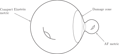
Figure 0.1. The approximate metric.

Since both $g_{Z}$ and $g_{N}$ are $B^{t}$-flat, this metric is an “approximate” $B^{t}$-flat metric, with vanishing $B^{t}$ tensor away from the “damage zone”, where cutoff functions were used.

0.43. Lyapunov-Schmidt reduction

In general, there are several degrees of freedom in this approximate metric.

• The scaling parameter $a$ ($1$-dimensional).

• Rotational freedom when attaching ($6$-dimensional).

• Freedom to move the base points of either factor ($8$-dimensional).

There are a total of 15 gluing parameters, which yield a 15-dimensional space of “approximate” kernel of the linearized operator. Using a Lyapunov-Schmidt reduction argument, one can reduce the problem to that of finding a zero of the Kuranishi map

(0.250) $$\Psi:U\subset\mathbb{R}^{15}\rightarrow\mathbb{R}^{15}.$$

• It is crucial to use certain weighted norms to find a bounded right inverse for the linearized operator.

• This 15-dimensional problem is too difficult in general. We will take advantage of various symmetries in order to reduce to only $1$ free parameter: the scaling parameter $a$.

0.43.1. Technical theorem

The leading term of the Kuranishi map corresponding to the scaling parameter is given by:

Theorem 0.108 ([GV13]).

As $a\rightarrow 0$, then for any $\epsilon>0$,

(0.251) $$\Psi_{1} =\Big{(}\frac{2}{3}W(z_{0})\circledast W(y_{0})+4tR(z_{0})\mathrm{mass}(g_{N})\Big{)}\omega_{3}a^{4}+O(a^{6-\epsilon}),$$

where $\omega_{3}=Vol(S^{3})$, and the product of the Weyl tensors is given by

(0.252) $$W(z_{0})\circledast W(y_{0})=\sum_{ijkl}W_{ijkl}(z_{0})(W_{ijkl}(y_{0})+W_{ilkj}(y_{0})),$$

where $W_{ijkl}(\cdot)$ denotes the components of the Weyl tensor in a normal coordinate system at the corresponding point.

We note that the product $\circledast$ depends upon the coordinate systems chosen, and therefore in general depends upon a rotation parameter, and obviously on the base points of the gluing.

0.44. The building blocks

We next discuss the “building blocks” of the gluing construction.

0.44.1. The Fubini-Study metric

We let $(\mathbb{CP}^{2},g_{\rm{FS}})$ denote the Fubini-Study metric, scaled so that $Ric=6g$. We consider the following group actions.

Torus action:

(0.253) $$[z_{0},z_{1},z_{2}]\mapsto[z_{0},e^{i\theta_{1}}z_{1},e^{i\theta_{2}}z_{2}].$$

Flip symmetry:

(0.254) $$[z_{0},z_{1},z_{2}]\mapsto[z_{0},z_{2},z_{1}].$$

The Green’s function metric of the Fubini-Study metric $\hat{g}_{FS}$ is also known as the Burns metric, and is completely explicit (in fact, it is the case $n=1$ of (0.224)) with mass given by

(0.255) $$\mathrm{mass}(\hat{g}_{FS})=2.$$

0.44.2. The product metric

The next building block is $(S^{2}\times S^{2},g_{S^{2}\times S^{2}})$, the product of $2$-dimensional spheres of Gaussian curvature $1$, with $Ric=g$. We consider the following group actions.

Torus action:

(0.256) $$\text{Product of rotations fixing north and south poles}.$$

Flip symmetry:

(0.257) $$(p_{1},p_{2})\mapsto(p_{2},p_{1}).$$

The Green’s function metric $\hat{g}_{S^{2}\times S^{2}}$ of the product metric does not seem to have a known explicit description. We will denote

(0.258) $$m_{1}=\mathrm{mass}(\hat{g}_{S^{2}\times S^{2}}).$$

By the positive mass theorem of Schoen-Yau, $m_{1}>0$. Note that since $S^{2}\times S^{2}$ is spin, this also follows from Witten’s proof of the positive mass theorem. The value of $m_{1}$ has recently been determined:

Theorem 0.109 ([Via13c]).

The mass $m_{1}\sim.5872$ and may be written as an explicit infinite sum.

The explicit formula for the mass is lengthy, and will not be written here. We just note that this implies that $(-9m_{1})^{-1}\sim=-.1892$ so as a corollary we see that the manifold $S^{2}\times S^{2}\#\overline{\mathbb{CP}}^{2}$ admits a $B^{t}$-flat metrics for at least two different values of $t$. Note that it is shown in [GV13] that the metrics obtained in Theorem 0.107 are not Einstein, so these metrics are distinct from the Chen-LeBrun-Weber metric.

0.45. Remarks on the proof

We first remark that:

• We impose the toric symmetry and “flip” symmetry in order to reduce the number of free parameters to $1$ (only the scaling parameter). That is, we perform an equivariant gluing.

• The special value of $t_{0}$ is computed by

  $$\frac{2}{3}W(z_{0})\circledast W(y_{0})+4t_{0}R(z_{0})\mathrm{mass}(g_{N})=0.$$

  This choice of $t_{0}$ makes the leading term of the Kuranishi map vanish, and is furthermore a nondegenerate zero (if $R(z_{0})>0$; mass$(g_{N})>0$ by the positive mass theorem).

We next outline the spaces used in the construction of the naïve approximate metric:

• (i) $\mathbb{CP}^{2}\#\overline{\mathbb{CP}}^{2}$; the Fubini-Study metric with a Burns metric attached at one fixed point. This case admits a $U(2)$-action.

• (ii) $S^{2}\times S^{2}\#\overline{\mathbb{CP}}^{2}=\mathbb{CP}^{2}\#2\overline{\mathbb{CP}}^{2}$; the product metric on $S^{2}\times S^{2}$ with a Burns metric attached at one fixed point. Alternatively, we can view this as the Fubini-Study metric on $\mathbb{CP}^{2}$, with a Green’s function $S^{2}\times S^{2}$ metric attached at one fixed point. For this topology, we will therefore construct two different critical metrics. Both of these will have toric symmetry plus invariance under the flip symmetry.

• (iii) $S^{2}\times S^{2}\#S^{2}\times S^{2}$; the product metric on $S^{2}\times S^{2}$ with a Green’s function $S^{2}\times S^{2}$ metric attached at one fixed point. This metric is toric and flip-symmetric.

We note that an equivariant gluing is carried out – the metrics obtained in Theorem 0.107 retain the indicated symmetries.

By imposing other discrete symmetries, we can perform the gluing operation with more than one bubble. For example, we can find critical metrics on $\mathbb{CP}^{2}\#3\overline{\mathbb{CP}}^{2}$ $3\#S^{2}\times S^{2}$, $\mathbb{CP}^{2}\#3(S^{2}\times S^{2})$, $S^{2}\times S^{2}\#4\overline{\mathbb{CP}}^{2}$, and $5\#S^{2}\times S^{2}$ (see [GV13, Table 1.2]).

The product metric on $S^{2}\times S^{2}$ admits the quotient $S^{2}\times S^{2}/\mathbb{Z}_{2}$ where $\mathbb{Z}_{2}$ acts by the antipodal map on both factors. It is well-known that this quotient is diffeomorphic to $G(2,4)$, the Grassmannian of $2$-planes in $\mathbb{R}^{4}$, see for example [ST69]. Another quotient is $\mathbb{RP}^{2}\times\mathbb{RP}^{2}$. The product metric descends to an Einstein metric on both of these quotients. We can also use these quotient spaces as building blocks to obtain non-simply connected examples. We do not list all of the examples here, but just note that we find a critical metric on $G(2,4)\#G(2,4)$, which has infinite fundamental group, and therefore does not admit any positive Einstein metric by Myers’ Theorem. For the complete list of non-simply-connected examples, see [GV13, Table 1.3, Table B.1].

0.45.1. Ellipticity and gauging

The $B^{t}$-flat equations are not elliptic due to diffeomorphism invariance. A gauging procedure analogous to the Bianchi gauge is used. This was already discussed above in Lecture 0.76, with the following note. From (0.121), we can write

(0.259) $$\mathcal{F}_{\tau}=16\pi^{2}\chi(M)+\frac{1}{2}\mathcal{B}_{2(\tau+\frac{1}{3})}.$$

Taking gradients, we obtain the relation

(0.260) $$\nabla\mathcal{B}_{t}=2\nabla\mathcal{F}_{\frac{t}{2}-\frac{1}{3}}.$$

It follows from the formula for $P$ that the linearized operator is given by

(0.261) $$S^{t}h=(B^{\prime}+tC^{\prime})h+\mathcal{K}_{g}\delta_{g}\mathcal{K}_{g}\delta_{g}\overset{\circ}{h},$$

where $B^{\prime}$ and $C^{\prime}$ are the linearizations of $B$ and $C$ respectively. Therefore the discussion in Lecture 0.76 applies, with $\tau$ replaced by $\frac{t}{2}-\frac{1}{3}$.

0.45.2. Rigidity

The rigidity results we need were discussed above. We mention here the resulting linearized operator as we change $\tau\rightarrow t$. For $h$ transverse-traceless (TT), the linearized operator at an Einstein metric is given by

(0.262) $$S^{t}h=\Big{(}\Delta_{L}+\frac{1}{2}R\Big{)}\Big{(}\Delta_{L}+\Big{(}\frac{1}{3}+t\Big{)}R\Big{)}h.$$

Next, for $h=fg$, we have

(0.263) $$tr_{g}(S^{t}h)=6t(3\Delta+R)(\Delta f).$$

The above rigidity results, Theorems 0.87 and 0.88, are then as follows (stated in terms of $t$ instead of $\tau$).

Theorem 0.110 ([GV11]).

On $(\mathbb{CP}^{2},g_{\rm{FS}})$, $H^{1}_{t}=\{0\}$ provided that $t<1$.

For the case of the product metric:

Theorem 0.111 ([GV11]).

On $(S^{2}\times S^{2},g_{S^{2}\times S^{2}})$, $H^{1}_{t}=\{0\}$ provided that $t<2/3$ and $t\neq-1/3$. If $t=-1/3$, then $H^{1}_{t}$ is one-dimensional and spanned by the element $g_{1}-g_{2}$.

In relation to Theorem 0.107, the positive mass theorem says that $t_{0}<0$, so luckily we are in the rigidity range of the factors. Consequently, there is no cokernel arising from deformations of the building blocks.

0.45.3. Refined approximate metric

The approximate metric described above is not good enough. It must be improved by matching up leading terms of the metrics by solving certain auxiliary linear equations, so that the cutoff function disappears from the leading term. This step is inspired by the work of Biquard mentioned above. Let $(Z,g_{Z})$ be the compact metric. In Riemannian normal coordinates,

(0.264) $$(g_{Z})_{ij}(z)=\delta_{ij}-\frac{1}{3}R_{ikjl}(z_{0})z^{k}z^{l}+O^{(4)}(|z|^{4})_{ij}$$

as $z\rightarrow z_{0}$.

Let $(N,g_{N})$ be the Green’s function metric of $(Y,g_{Y})$, then we have

(0.265) $$(g_{N})_{ij}(x) =\delta_{ij}-\frac{1}{3}R_{ikjl}(y_{0})\frac{x^{k}x^{l}}{|x|^{4}}+2A\frac{1}{|x|^{2}}\delta_{ij}+O^{(4)}(|x|^{-4+\epsilon})$$

as $|x|\rightarrow\infty$, for any $\epsilon>0$. Note that the constant $A$ is given by

(0.266) $$\mathrm{mass}(g_{N})=12A-R(y_{0})/12.$$

We consider $a^{-4}g_{Z}$ and let $z=a^{2}x$, then we have

(0.267) $$a^{-4}(g_{Z})_{ij}(x)=\delta_{ij}-a^{4}\frac{1}{3}R_{ikjl}(z_{0})x^{k}x^{l}+\cdots.$$

Note that the second order terms do not agree. One needs to construct new metrics on the factors so that these terms agree. This is done by solving the linearized equation on each factor with prescribed leading term the second order term of the other metric. We will describe this procedure next.

0.45.4. The obstruction

On $(N,g_{N})$, one would like to solve

(0.268) $$\begin{split}S^{t}\tilde{h}&=0\\ \tilde{h}&=-a^{4}\frac{1}{3}R_{ikjl}(z_{0})x^{k}x^{l}+O(|x|^{\epsilon}),\end{split}$$

as $x\rightarrow\infty$. However, it turns out this equation is obstructed, so there is not necessarily a solution. However, using some Fredholm theory in weighted spaces, it turns out that one can solve the modified equation

$$S^{t}\tilde{h}=\lambda\cdot k_{1},$$

where $k_{1}$ pairs nontrivially with the decaying cokernel $o_{1}$ on the AF space $(N,g_{N})$. (There is also a considerable amount of work involved in order to prove that the space of decaying cokernel is $1$-dimensional; the symmetries are crucial for this.)

• A similar procedure is carried out on the compact factor, except this is unobstructed (since the compact factor is rigid), so this does not contribute to the leading term of the Kuranishi map.

The leading term is the computed by the following. Pairing with the cokernel element $o_{1}$,

$$\lambda =\lim_{r\rightarrow\infty}\int_{B(r)}\langle S\tilde{h},o_{1}\rangle$$

$$=\lim_{r\rightarrow\infty}(\mathrm{\ spherical\ boundary\ integrals}).$$

This limit can be computed explicitly using the expansion of the cokernel element

(0.269) $$(o_{1})_{ij}=\frac{2}{3}W_{ikjl}(y_{0})\frac{x^{k}x^{l}}{|x|^{4}}+fg_{ij}+O(|x|^{-4+\epsilon})$$

as $x\rightarrow\infty$, where $f$ satisfies

(0.270) $$\Delta f=-\frac{1}{3}\langle Ric,o_{1}\rangle,$$

together with the expansion

(0.271) $$\tilde{h} =-a^{4}\frac{1}{3}R_{ikjl}(z_{0})x^{k}x^{l}+O(|x|^{\epsilon}),$$

as $x\rightarrow\infty$.

The complete computation is very lengthy, and we refer to [GV13] for the details.

0.45.5. Final remarks

The proof shows that there is a dichotomy. Either

• (i) there is a critical metric at exactly the critical $t_{0}$, in which case there would necessarily be a 1-dimensional moduli space of solutions for this fixed $t_{0}$, or

• (ii) for each value of the gluing parameter $a$ sufficiently small, there will be a critical metric for a corresponding value of $t_{0}=t_{0}(a)$. The dependence of $t_{0}$ on $a$ will depend on the next term in the expansion of the Kuranishi map.

References

- [AB03] Kazuo Akutagawa and Boris Botvinnik, Yamabe metrics on cylindrical manifolds, Geom. Funct. Anal. 13 (2003), no. 2, 259–333. MR 1982146 (2004e:53051)
- [AB04] by same author, The Yamabe invariants of orbifolds and cylindrical manifolds, and -harmonic spinors, J. Reine Angew. Math. 574 (2004), 121–146. MR 2099112 (2005g:53055)
- [ACG03] V. Apostolov, D. M. J. Calderbank, and P. Gauduchon, The geometry of weakly self-dual Kähler surfaces, Compositio Math. 135 (2003), no. 3, 279–322. MR 1956815 (2004f:53045)
- [ADH13] Bernd Ammann, Mattias Dahl, and Emmanuel Humbert, Smooth Yamabe invariant and surgery, J. Differential Geom. 94 (2013), no. 1, 1–58. MR 3031859
- [AHS78] M. F. Atiyah, N. J. Hitchin, and I. M. Singer, Self-duality in four-dimensional Riemannian geometry, Proc. Roy. Soc. London Ser. A 362 (1978), no. 1711, 425–461. MR 506229 (80d:53023)
- [AIL07] Kazuo Akutagawa, Masashi Ishida, and Claude LeBrun, Perelman’s invariant, Ricci flow, and the Yamabe invariants of smooth manifolds, Arch. Math. (Basel) 88 (2007), no. 1, 71–76. MR 2289603 (2007j:53070)
- [Aku94] Kazuo Akutagawa, Yamabe metrics of positive scalar curvature and conformally flat manifolds, Differential Geom. Appl. 4 (1994), no. 3, 239–258. MR 95i:58046
- [Aku12] by same author, Computations of the orbifold Yamabe invariant, Math. Z. 271 (2012), no. 3-4, 611–625. MR 2945574
- [And89] Michael T. Anderson, Ricci curvature bounds and Einstein metrics on compact manifolds, J. Amer. Math. Soc. 2 (1989), no. 3, 455–490. MR 90g:53052
- [And97] by same author, Extrema of curvature functionals on the space of metrics on -manifolds, Calc. Var. Partial Differential Equations 5 (1997), no. 3, 199–269. MR 1438146 (98a:58041)
- [And01] by same author, Extrema of curvature functionals on the space of metrics on 3-manifolds. II, Calc. Var. Partial Differential Equations 12 (2001), no. 1, 1–58. MR 1808106 (2002a:58012)
- [And10] by same author, A survey of Einstein metrics on 4-manifolds, Handbook of geometric analysis, No. 3, Adv. Lect. Math. (ALM), vol. 14, Int. Press, Somerville, MA, 2010, pp. 1–39. MR 2743446 (2012a:53071)
- [AP06] Claudio Arezzo and Frank Pacard, Blowing up and desingularizing constant scalar curvature Kähler manifolds, Acta Math. 196 (2006), no. 2, 179–228. MR 2275832 (2007i:32018)
- [AP09] by same author, Blowing up Kähler manifolds with constant scalar curvature. II, Ann. of Math. (2) 170 (2009), no. 2, 685–738. MR 2552105 (2010m:32025)
- [APS11] Claudio Arezzo, Frank Pacard, and Michael Singer, Extremal metrics on blowups, Duke Math. J. 157 (2011), no. 1, 1–51. MR 2783927 (2012k:32024)
- [Aub76] Thierry Aubin, Équations différentielles non linéaires et problème de Yamabe concernant la courbure scalaire, J. Math. Pures Appl. (9) 55 (1976), no. 3, 269–296.
- [Aub78] by same author, Équations du type Monge-Ampère sur les variétés kählériennes compactes, Bull. Sci. Math. (2) 102 (1978), no. 1, 63–95. MR 494932 (81d:53047)
- [Aub98] by same author, Some nonlinear problems in Riemannian geometry, Springer-Verlag, Berlin, 1998.
- [AV12a] Antonio G. Ache and Jeff A. Viaclovsky, Obstruction-flat asymptotically locally Euclidean metrics, Geom. Funct. Anal. 22 (2012), no. 4, 832–877.
- [AV12b] by same author, Asymptotics of the self-dual deformation complex, arXiv.org:1201.1028, to appear in Journal of Geometric Analysis, 2012.
- [Bac21] R. Bach, Zur weylschen relativitatstheorie und der weylschen erweiterung des krummungstensorbegriffs, Math. Zeit. 9 (1921), 112–135.
- [Bar86] Robert Bartnik, The mass of an asymptotically flat manifold, Comm. Pure Appl. Math. 39 (1986), no. 5, 661–693. MR 849427 (88b:58144)
- [BC64] Richard L. Bishop and Richard J. Crittenden, Geometry of manifolds, Academic Press, New York, 1964. MR 29 #6401
- [BCG95] G. Besson, G. Courtois, and S. Gallot, Entropies et rigidités des espaces localement symétriques de courbure strictement négative, Geom. Funct. Anal. 5 (1995), no. 5, 731–799. MR 1354289 (96i:58136)
- [BE69] M. Berger and D. Ebin, Some decompositions of the space of symmetric tensors on a Riemannian manifold, J. Differential Geometry 3 (1969), 379–392. MR 0266084 (42 #993)
- [Ber70] Marcel Berger, Quelques formules de variation pour une structure riemannienne, Ann. Sci. École Norm. Sup. (4) 3 (1970), 285–294. MR 0278238 (43 #3969)
- [Bes08] Arthur L. Besse, Einstein manifolds, Classics in Mathematics, Springer-Verlag, Berlin, 2008, Reprint of the 1987 edition. MR 2371700 (2008k:53084)
- [BG08] Thomas P. Branson and A. Rod Gover, Origins, applications and generalisations of the -curvature, Acta Appl. Math. 102 (2008), no. 2-3, 131–146. MR 2407527 (2010a:53025)
- [Biq13a] Olivier Biquard, Désingularisation de métriques d’Einstein. I, Invent. Math. 192 (2013), no. 1, 197–252. MR 3032330
- [Biq13b] by same author, Désingularisation de métriques d’Einstein. II, arXiv.org:1311.0956, 2013.
- [BKN89] Shigetoshi Bando, Atsushi Kasue, and Hiraku Nakajima, On a construction of coordinates at infinity on manifolds with fast curvature decay and maximal volume growth, Invent. Math. 97 (1989), no. 2, 313–349. MR 90c:53098
- [BL09] Hubert L. Bray and Dan A. Lee, On the Riemannian Penrose inequality in dimensions less than eight, Duke Math. J. 148 (2009), no. 1, 81–106. MR 2515101 (2010f:53051)
- [Bla00] David E. Blair, Spaces of metrics and curvature functionals, Handbook of differential geometry, Vol. I, North-Holland, Amsterdam, 2000, pp. 153–185.
- [BM09] Simon Brendle and Fernando C. Marques, Blow-up phenomena for the Yamabe equation. II, J. Differential Geom. 81 (2009), no. 2, 225–250. MR 2472174 (2010k:53050)
- [BM11] Olivier Biquard and Vincent Minerbe, A Kummer construction for gravitational instantons, Comm. Math. Phys. 308 (2011), no. 3, 773–794. MR 2855540 (2012m:53101)
- [BN04] Hubert L. Bray and André Neves, Classification of prime 3-manifolds with Yamabe invariant greater than , Ann. of Math. (2) 159 (2004), no. 1, 407–424. MR 2052359 (2005f:53048a)
- [Bog78] F. A. Bogomolov, Hamiltonian Kählerian manifolds, Dokl. Akad. Nauk SSSR 243 (1978), no. 5, 1101–1104.
- [Bra01] Hubert L. Bray, Proof of the Riemannian Penrose inequality using the positive mass theorem, J. Differential Geom. 59 (2001), no. 2, 177–267. MR 1908823 (2004j:53046)
- [Bre05] Simon Brendle, Convergence of the Yamabe flow for arbitrary initial energy, J. Differential Geom. 69 (2005), no. 2, 217–278. MR 2168505 (2006e:53119)
- [Bre07] by same author, Convergence of the Yamabe flow in dimension 6 and higher, Invent. Math. 170 (2007), no. 3, 541–576. MR 2357502 (2008k:53136)
- [Bre08] by same author, Blow-up phenomena for the Yamabe equation, J. Amer. Math. Soc. 21 (2008), no. 4, 951–979. MR 2425176 (2009m:53084)
- [BWZ04] C. Böhm, M. Wang, and W. Ziller, A variational approach for compact homogeneous Einstein manifolds, Geom. Funct. Anal. 14 (2004), no. 4, 681–733. MR 2084976 (2005g:53074)
- [Cal82] Eugenio Calabi, Extremal Kähler metrics, Seminar on Differential Geometry, Ann. of Math. Stud., vol. 102, Princeton Univ. Press, Princeton, N.J., 1982, pp. 259–290. MR 645743 (83i:53088)
- [Cal85] by same author, Extremal Kähler metrics. II, Differential geometry and complex analysis, Springer, Berlin, 1985, pp. 95–114. MR 780039 (86h:53067)
- [Car98] Gilles Carron, Une suite exacte en -cohomologie, Duke Math. J. 95 (1998), no. 2, 343–372.
- [CG72] Jeff Cheeger and Detlef Gromoll, The splitting theorem for manifolds of nonnegative Ricci curvature, J. Differential Geometry 6 (1971/72), 119–128. MR 0303460 (46 #2597)
- [CGY02a] Sun-Yung A. Chang, Matthew J. Gursky, and Paul Yang, An a priori estimate for a fully nonlinear equation on four-manifolds, J. Anal. Math. 87 (2002), 151–186, Dedicated to the memory of Thomas H. Wolff. MR 1945280 (2003k:53036)
- [CGY02b] Sun-Yung A. Chang, Matthew J. Gursky, and Paul C. Yang, An equation of Monge-Ampère type in conformal geometry, and four-manifolds of positive Ricci curvature, Ann. of Math. (2) 155 (2002), no. 3, 709–787. MR 1923964 (2003j:53048)
- [Che70] Jeff Cheeger, Finiteness theorems for Riemannian manifolds, Amer. J. Math. 92 (1970), 61–74. MR 0263092 (41 #7697)
- [Che09] Szu-Yu Sophie Chen, Optimal curvature decays on asymptotically locally euclidean manifolds, arXiv.org:0911.5538, 2009.
- [CLW08] Xiuxiong Chen, Claude Lebrun, and Brian Weber, On conformally Kähler, Einstein manifolds, J. Amer. Math. Soc. 21 (2008), no. 4, 1137–1168.
- [CS04] David M. J. Calderbank and Michael A. Singer, Einstein metrics and complex singularities, Invent. Math. 156 (2004), no. 2, 405–443.
- [CS06] by same author, Toric self-dual Einstein metrics on compact orbifolds, Duke Math. J. 133 (2006), no. 2, 237–258. MR 2225692 (2007g:53041)
- [CT94] Jeff Cheeger and Gang Tian, On the cone structure at infinity of Ricci flat manifolds with Euclidean volume growth and quadratic curvature decay, Invent. Math. 118 (1994), no. 3, 493–571.
- [CT06] by same author, Curvature and injectivity radius estimates for Einstein 4-manifolds, J. Amer. Math. Soc. 19 (2006), no. 2, 487–525 (electronic). MR 2188134 (2006i:53042)
- [CW11] Xiuxiong Chen and Brian Weber, Moduli spaces of critical Riemannian metrics with norm curvature bounds, Adv. Math. 226 (2011), no. 2, 1307–1330.
- [Der83] Andrzej Derdziński, Self-dual Kähler manifolds and Einstein manifolds of dimension four, Compositio Math. 49 (1983), no. 3, 405–433. MR 707181 (84h:53060)
- [DF89] S. Donaldson and R. Friedman, Connected sums of self-dual manifolds and deformations of singular spaces, Nonlinearity 2 (1989), no. 2, 197–239.
- [dLPZ12] L. L. de Lima, P. Piccione, and M. Zedda, A note on the uniqueness of solutions for the Yamabe problem, Proc. Amer. Math. Soc. 140 (2012), no. 12, 4351–4357. MR 2957225
- [DM08] Zindine Djadli and Andrea Malchiodi, Existence of conformal metrics with constant -curvature, Ann. of Math. (2) 168 (2008), no. 3, 813–858. MR 2456884 (2009h:53074)
- [DN55] Avron Douglis and Louis Nirenberg, Interior estimates for elliptic systems of partial differential equations, Comm. Pure Appl. Math. 8 (1955), 503–538.
- [Don10] Simon Donaldson, Calabi-Yau metrics on Kummer surfaces as a model glueing problem, arXiv:1007.421, 2010.
- [Don11] by same author, Riemann surfaces, Oxford Graduate Texts in Mathematics, vol. 22, Oxford University Press, Oxford, 2011. MR 2856237
- [DWW05] Xianzhe Dai, Xiaodong Wang, and Guofang Wei, On the stability of Riemannian manifold with parallel spinors, Invent. Math. 161 (2005), no. 1, 151–176.
- [Ebi68] David G. Ebin, On the space of Riemannian metrics, Bull. Amer. Math. Soc. 74 (1968), 1001–1003. MR 0231410 (37 #6965)
- [EE69] Clifford J. Earle and James Eells, A fibre bundle description of Teichmüller theory, J. Differential Geometry 3 (1969), 19–43. MR 0276999 (43 #2737a)
- [EH79] Tohru Eguchi and Andrew J. Hanson, Self-dual solutions to Euclidean gravity, Ann. Physics 120 (1979), no. 1, 82–106.
- [Flo91] Andreas Floer, Self-dual conformal structures on , J. Differential Geom. 33 (1991), no. 2, 551–573.
- [FM77] Arthur E. Fischer and Jerrold E. Marsden, The manifold of conformally equivalent metrics, Canad. J. Math. 29 (1977), no. 1, 193–209. MR 0445537 (56 #3877)
- [FM93] Akito Futaki and Toshiki Mabuchi, Uniqueness and periodicity of extremal Kähler vector fields, Proceedings of GARC Workshop on Geometry and Topology ’93 (Seoul, 1993), Lecture Notes Ser., vol. 18, Seoul Nat. Univ., Seoul, 1993, pp. 217–239. MR 1270938 (95c:32028)
- [Fuj00] Akira Fujiki, Compact self-dual manifolds with torus actions, J. Differential Geom. 55 (2000), no. 2, 229–324. MR 1847312 (2002k:57085)
- [Fut83] A. Futaki, An obstruction to the existence of Einstein Kähler metrics, Invent. Math. 73 (1983), no. 3, 437–443. MR 718940 (84j:53072)
- [Fut88] Akito Futaki, Kähler-Einstein metrics and integral invariants, Lecture Notes in Mathematics, vol. 1314, Springer-Verlag, Berlin, 1988. MR 947341 (90a:53053)
- [GH78] G. W. Gibbons and S. W. Hawking, Gravitational multi-instantons, Physics Letters B 78 (1978), no. 4, 430–432.
- [GL98] M. J. Gursky and C. LeBrun, Yamabe invariants and structures, Geom. Funct. Anal. 8 (1998), no. 6, 965–977. MR 1664788 (99k:53078)
- [Gra09] C. Robin Graham, Extended obstruction tensors and renormalized volume coefficients, Adv. Math. 220 (2009), no. 6, 1956–1985. MR 2493186 (2010e:53060)
- [Gro07] Misha Gromov, Metric structures for Riemannian and non-Riemannian spaces, english ed., Modern Birkhäuser Classics, Birkhäuser Boston, Inc., Boston, MA, 2007, Based on the 1981 French original, With appendices by M. Katz, P. Pansu and S. Semmes, Translated from the French by Sean Michael Bates. MR 2307192 (2007k:53049)
- [Gur98] Matthew J. Gursky, The Weyl functional, de Rham cohomology, and Kähler-Einstein metrics, Ann. of Math. (2) 148 (1998), no. 1, 315–337. MR 1652920 (99i:58036)
- [Gur00] by same author, Four-manifolds with and Einstein constants of the sphere, Math. Ann. 318 (2000), no. 3, 417–431. MR 1800764 (2002c:53074)
- [GV01] Matthew J. Gursky and Jeff A. Viaclovsky, A new variational characterization of three-dimensional space forms, Invent. Math. 145 (2001), no. 2, 251–278. MR 1872547 (2002j:53039)
- [GV03] by same author, A fully nonlinear equation on four-manifolds with positive scalar curvature, J. Differential Geom. 63 (2003), no. 1, 131–154. MR 2015262 (2004h:53052)
- [GV07] by same author, Prescribing symmetric functions of the eigenvalues of the Ricci tensor, Ann. of Math. (2) 166 (2007), no. 2, 475–531. MR 2373147 (2008k:53068)
- [GV11] by same author, Rigidity and stability of Einstein metrics for quadratic curvature functionals, arXiv.org:1105.4648, to appear in Crelle’s Journal, 2011.
- [GV13] by same author, Critical metrics on connected sums of Einstein four-manifolds, preprint, arXiv.org:1303.0827, 2013.
- [GW00] Mark Gross and P. M. H. Wilson, Large complex structure limits of surfaces, J. Differential Geom. 55 (2000), no. 3, 475–546. MR 1863732 (2003a:32042)
- [GW03] Pengfei Guan and Guofang Wang, A fully nonlinear conformal flow on locally conformally flat manifolds, J. Reine Angew. Math. 557 (2003), 219–238. MR 1978409 (2004e:53101)
- [GW06] Yuxin Ge and Guofang Wang, On a fully nonlinear Yamabe problem, Ann. Sci. École Norm. Sup. (4) 39 (2006), no. 4, 569–598. MR 2290138 (2007k:53040)
- [Ham82] Richard S. Hamilton, Three-manifolds with positive Ricci curvature, J. Differential Geom. 17 (1982), no. 2, 255–306. MR 84a:53050
- [Hei12] Hans-Joachim Hein, Gravitational instantons from rational elliptic surfaces, J. Amer. Math. Soc. 25 (2012), no. 2, 355–393. MR 2869021
- [Hir95] Friedrich Hirzebruch, Topological methods in algebraic geometry, Classics in Mathematics, Springer-Verlag, Berlin, 1995, Translated from the German and Appendix One by R. L. E. Schwarzenberger, With a preface to the third English edition by the author and Schwarzenberger, Appendix Two by A. Borel, Reprint of the 1978 edition. MR 1335917 (96c:57002)
- [Hit74] Nigel Hitchin, Compact four-dimensional Einstein manifolds, J. Differential Geometry 9 (1974), 435–441.
- [Hit79] N. J. Hitchin, Polygons and gravitons, Math. Proc. Cambridge Philos. Soc. 85 (1979), no. 3, 465–476.
- [Hon06] Nobuhiro Honda, Non-Moishezon twistor spaces of with non-trivial automorphism group, Trans. Amer. Math. Soc. 358 (2006), no. 5, 1897–1920 (electronic). MR 2197434 (2006j:32020)
- [Hon07] by same author, Self-dual metrics and twenty-eight bitangents, J. Differential Geom. 75 (2007), no. 2, 175–258. MR 2286821 (2008c:32029)
- [Ito93] Mitsuhiro Itoh, Moduli of half conformally flat structures, Math. Ann. 296 (1993), no. 4, 687–708.
- [Ito95] by same author, The Weitzenböck formula for the Bach operator, Nagoya Math. J. 137 (1995), 149–181.
- [JM87] Dennis Johnson and John J. Millson, Deformation spaces associated to compact hyperbolic manifolds, Discrete groups in geometry and analysis (New Haven, Conn., 1984), Progr. Math., vol. 67, Birkhäuser Boston, Boston, MA, 1987, pp. 48–106.
- [Joy95] Dominic D. Joyce, Explicit construction of self-dual -manifolds, Duke Math. J. 77 (1995), no. 3, 519–552.
- [Joy96] by same author, Compact Riemannian -manifolds with holonomy . I, II, J. Differential Geom. 43 (1996), no. 2, 291–328, 329–375. MR 1424428 (97m:53084)
- [Joy99] Dominic Joyce, A new construction of compact 8-manifolds with holonomy , J. Differential Geom. 53 (1999), no. 1, 89–130. MR 1776092 (2002a:53063)
- [Kat94] Shin Kato, Examples of non-Einstein Yamabe metrics with positive scalar curvature, Tokyo J. Math. 17 (1994), no. 1, 187–189. MR 1279579 (95f:53078)
- [KK92] A. D. King and D. Kotschick, The deformation theory of anti-self-dual conformal structures, Math. Ann. 294 (1992), no. 4, 591–609.
- [KMS09] M. A. Khuri, F. C. Marques, and R. M. Schoen, A compactness theorem for the Yamabe problem, J. Differential Geom. 81 (2009), no. 1, 143–196. MR 2477893 (2010e:53065)
- [Kob85] Osamu Kobayashi, On a conformally invariant functional of the space of Riemannian metrics, J. Math. Soc. Japan 37 (1985), no. 3, 373–389.
- [Kob87] by same author, Scalar curvature of a metric with unit volume, Math. Ann. 279 (1987), no. 2, 253–265. MR 919505 (89a:53048)
- [Koi78] Norihito Koiso, Nondeformability of Einstein metrics, Osaka J. Math. 15 (1978), no. 2, 419–433. MR 504300 (81h:53046)
- [Koi80] by same author, Rigidity and stability of Einstein metrics—the case of compact symmetric spaces, Osaka J. Math. 17 (1980), no. 1, 51–73.
- [Koi82] by same author, Rigidity and infinitesimal deformability of Einstein metrics, Osaka J. Math. 19 (1982), no. 3, 643–668.
- [Kro89a] P. B. Kronheimer, The construction of ALE spaces as hyper-Kähler quotients, J. Differential Geom. 29 (1989), no. 3, 665–683.
- [Kro89b] by same author, A Torelli-type theorem for gravitational instantons, J. Differential Geom. 29 (1989), no. 3, 685–697.
- [KS01] A. Kovalev and M. Singer, Gluing theorems for complete anti-self-dual spaces, Geom. Funct. Anal. 11 (2001), no. 6, 1229–1281.
- [KT87] Ryoichi Kobayashi and Andrey N. Todorov, Polarized period map for generalized surfaces and the moduli of Einstein metrics, Tohoku Math. J. (2) 39 (1987), no. 3, 341–363. MR 902574 (89g:32029)
- [Küh88] Wolfgang Kühnel, Conformal transformations between Einstein spaces, Conformal geometry (Bonn, 1985/1986), Aspects Math., E12, Vieweg, Braunschweig, 1988, pp. 105–146. MR 979791 (90b:53055)
- [Laf83] Jacques Lafontaine, Modules de structures conformes plates et cohomologie de groupes discrets, C. R. Acad. Sci. Paris Sér. I Math. 297 (1983), no. 13, 655–658.
- [LeB88] Claude LeBrun, Counter-examples to the generalized positive action conjecture, Comm. Math. Phys. 118 (1988), no. 4, 591–596.
- [LeB91] by same author, Explicit self-dual metrics on , J. Differential Geom. 34 (1991), no. 1, 223–253.
- [LeB92] by same author, Twistors, Kähler manifolds, and bimeromorphic geometry. I, J. Amer. Math. Soc. 5 (1992), no. 2, 289–316.
- [LeB95] by same author, Einstein metrics and Mostow rigidity, Math. Res. Lett. 2 (1995), no. 1, 1–8. MR 1312972 (95m:53067)
- [LeB97] by same author, Yamabe constants and the perturbed Seiberg-Witten equations, Comm. Anal. Geom. 5 (1997), no. 3, 535–553. MR 1487727 (98j:58032)
- [LeB99] by same author, Einstein metrics and the Yamabe problem, Trends in mathematical physics (Knoxville, TN, 1998), AMS/IP Stud. Adv. Math., vol. 13, Amer. Math. Soc., Providence, RI, 1999, pp. 353–376. MR 1708770 (2000f:53057)
- [LeB01] by same author, Ricci curvature, minimal volumes, and Seiberg-Witten theory, Invent. Math. 145 (2001), no. 2, 279–316.
- [LeB04] by same author, Curvature functionals, optimal metrics, and the differential topology of 4-manifolds, Different faces of geometry, Int. Math. Ser. (N. Y.), vol. 3, Kluwer/Plenum, New York, 2004, pp. 199–256. MR 2102997 (2005h:53055)
- [Lic58] André Lichnerowicz, Géométrie des groupes de transformations, Travaux et Recherches Mathématiques, III. Dunod, Paris, 1958. MR 0124009 (23 #A1329)
- [LL03] Aobing Li and Yanyan Li, On some conformally invariant fully nonlinear equations, Comm. Pure Appl. Math. 56 (2003), no. 10, 1416–1464. MR 1988895 (2004e:35072)
- [LM08] Claude LeBrun and Bernard Maskit, On optimal 4-dimensional metrics, J. Geom. Anal. 18 (2008), no. 2, 537–564.
- [LP87] John M. Lee and Thomas H. Parker, The Yamabe problem, Bull. Amer. Math. Soc. (N.S.) 17 (1987), no. 1, 37–91.
- [LS93] Claude LeBrun and Santiago R. Simanca, On the Kähler classes of extremal metrics, Geometry and global analysis (Sendai, 1993), Tohoku Univ., Sendai, 1993, pp. 255–271. MR 1361191 (96h:58037)
- [LS94] Claude LeBrun and Michael Singer, A Kummer-type construction of self-dual -manifolds, Math. Ann. 300 (1994), no. 1, 165–180.
- [LV12] Michael T. Lock and Jeff A. Viaclovsky, Anti-self-dual orbifolds with cyclic quotient singularities, arXiv:1205.4059, (to appear in Journal of the European Mathematical Society), 2012.
- [Min10] Vincent Minerbe, On the asymptotic geometry of gravitational instantons, Ann. Sci. Éc. Norm. Supér. (4) 43 (2010), no. 6, 883–924. MR 2778451
- [MØ13] Niels Martin Møller and Bent Ørsted, Rigidity of conformal functionals on spheres, International Mathematics Research Notices (2013), 1–38.
- [Mos68] G. D. Mostow, Quasi-conformal mappings in -space and the rigidity of hyperbolic space forms, Inst. Hautes Études Sci. Publ. Math. (1968), no. 34, 53–104. MR 0236383 (38 #4679)
- [Nak88] Hiraku Nakajima, Hausdorff convergence of Einstein -manifolds, J. Fac. Sci. Univ. Tokyo Sect. IA Math. 35 (1988), no. 2, 411–424. MR 90e:53063
- [Oba62] Morio Obata, Certain conditions for a Riemannian manifold to be isometric with a sphere, J. Math. Soc. Japan 14 (1962), 333–340. MR 0142086 (25 #5479)
- [Oba72] by same author, The conjectures on conformal transformations of Riemannian manifolds, J. Differential Geometry 6 (1971/72), 247–258. MR 0303464 (46 #2601)
- [Omo70] Hideki Omori, On the group of diffeomorphisms on a compact manifold, Global Analysis (Proc. Sympos. Pure Math., Vol. XV, Berkeley, Calif., 1968), Amer. Math. Soc., Providence, R.I., 1970, pp. 167–183. MR 0271983 (42 #6864)
- [Pag78a] Don Page, A compact rotating gravitational instanton, Physics Letters B 79 (1978), no. 3, 235 – 238.
- [Pag78b] Don N. Page, A physical picture of the gravitational instanton, Physics Letters B 80 (1978), no. 1-2, 55 – 57.
- [Pet00] Jimmy Petean, The Yamabe invariant of simply connected manifolds, J. Reine Angew. Math. 523 (2000), 225–231. MR 1762961 (2001g:53075)
- [Poo86] Y. Sun Poon, Compact self-dual manifolds with positive scalar curvature, J. Differential Geom. 24 (1986), no. 1, 97–132.
- [Poo92] by same author, On the algebraic structure of twistor spaces, J. Differential Geom. 36 (1992), no. 2, 451–491.
- [RS05] Yann Rollin and Michael Singer, Non-minimal scalar-flat Kähler surfaces and parabolic stability, Invent. Math. 162 (2005), no. 2, 235–270. MR 2199006 (2007b:32035)
- [Sch84] Richard M. Schoen, Conformal deformation of a Riemannian metric to constant scalar curvature, J. Differential Geom. 20 (1984), no. 2, 479–495.
- [Sch89] by same author, Variational theory for the total scalar curvature functional for Riemannian metrics and related topics, Topics in calculus of variations (Montecatini Terme, 1987), Lecture Notes in Math., vol. 1365, Springer, Berlin, 1989, pp. 120–154.
- [Sim85] Leon Simon, Isolated singularities of extrema of geometric variational problems, Harmonic mappings and minimal immersions (Montecatini, 1984), Lecture Notes in Math., vol. 1161, Springer, Berlin, 1985, pp. 206–277.
- [Smo05] N. K. Smolentsev, Spaces of Riemannian metrics, Sovrem. Mat. Prilozh. (2005), no. 31, Geometriya, 69–147. MR 2464555 (2010a:58015)
- [ST69] I. M. Singer and J. A. Thorpe, The curvature of -dimensional Einstein spaces, Global Analysis (Papers in Honor of K. Kodaira), Univ. Tokyo Press, Tokyo, 1969, pp. 355–365.
- [Str10] Jeffrey Streets, Asymptotic curvature decay and removal of singularities of Bach-flat metrics, Trans. Amer. Math. Soc. 362 (2010), no. 3, 1301–1324.
- [STW07] Wei-Min Sheng, Neil S. Trudinger, and Xu-Jia Wang, The Yamabe problem for higher order curvatures, J. Differential Geom. 77 (2007), no. 3, 515–553. MR 2362323 (2008i:53048)
- [Sun09] Chanyoung Sung, Surgery, Yamabe invariant, and Seiberg-Witten theory, J. Geom. Phys. 59 (2009), no. 2, 246–255. MR 2492194 (2010a:53054)
- [SY79] Richard M. Schoen and Shing Tung Yau, On the proof of the positive mass conjecture in general relativity, Comm. Math. Phys. 65 (1979), no. 1, 45–76.
- [SY81] by same author, Proof of the positive mass theorem. II, Comm. Math. Phys. 79 (1981), no. 2, 231–260.
- [SY88] by same author, Conformally flat manifolds, Kleinian groups and scalar curvature, Inventiones Mathematicae 92 (1988), no. 1, 47–71.
- [Tau92] Clifford Henry Taubes, The existence of anti-self-dual conformal structures, J. Differential Geom. 36 (1992), no. 1, 163–253. MR 1168984 (93j:53063)
- [Tho69] John A. Thorpe, Some remarks on the Gauss-Bonnet integral, J. Math. Mech. 18 (1969), 779–786.
- [Tia87] Gang Tian, Smoothness of the universal deformation space of compact Calabi-Yau manifolds and its Petersson-Weil metric, Mathematical aspects of string theory (San Diego, Calif., 1986), Adv. Ser. Math. Phys., vol. 1, World Sci. Publishing, Singapore, 1987, pp. 629–646.
- [Tia90] G. Tian, On Calabi’s conjecture for complex surfaces with positive first Chern class, Invent. Math. 101 (1990), no. 1, 101–172. MR 1055713 (91d:32042)
- [Tru68] Neil S. Trudinger, Remarks concerning the conformal deformation of Riemannian structures on compact manifolds, Ann. Scuola Norm. Sup. Pisa (3) 22 (1968), 265–274.
- [TV05a] Gang Tian and Jeff Viaclovsky, Bach-flat asymptotically locally Euclidean metrics, Invent. Math. 160 (2005), no. 2, 357–415.
- [TV05b] by same author, Moduli spaces of critical Riemannian metrics in dimension four, Adv. Math. 196 (2005), no. 2, 346–372.
- [TV08] by same author, Volume growth, curvature decay, and critical metrics, Comment. Math. Helv. 83 (2008), no. 4, 889–911.
- [TY87] Gang Tian and Shing-Tung Yau, Kähler-Einstein metrics on complex surfaces with , Comm. Math. Phys. 112 (1987), no. 1, 175–203. MR 904143 (88k:32070)
- [Uhl82a] Karen K. Uhlenbeck, Connections with bounds on curvature, Comm. Math. Phys. 83 (1982), no. 1, 31–42. MR 83e:53035
- [Uhl82b] by same author, Removable singularities in Yang-Mills fields, Comm. Math. Phys. 83 (1982), no. 1, 11–29. MR 83e:53034
- [Via00] Jeff A. Viaclovsky, Conformal geometry, contact geometry, and the calculus of variations, Duke Math. J. 101 (2000), no. 2, 283–316. MR 1738176 (2001b:53038)
- [Via06] Jeff Viaclovsky, Conformal geometry and fully nonlinear equations, Inspired by S. S. Chern, Nankai Tracts Math., vol. 11, World Sci. Publ., Hackensack, NJ, 2006, pp. 435–460. MR 2313345 (2008c:53030)
- [Via10] Jeff A. Viaclovsky, Monopole metrics and the orbifold Yamabe problem, Ann. Inst. Fourier (Grenoble) 60 (2010), no. 7, 2503–2543 (2011). MR 2866998 (2012m:53078)
- [Via13a] by same author, Einstein metrics and Yamabe invariants of weighted projective spaces, Tohoku Math. J. (2) 65 (2013), no. 2, 297–311. MR 3079291
- [Via13b] by same author, An index theorem on anti-self-dual orbifolds, Int. Math. Res. Not. IMRN (2013), no. 17, 3911–3930. MR 3096914
- [Via13c] by same author, The mass of the product of spheres, arXiv.org:1312.5287, to appear in Comm. Math. Phys., 2013.
- [Wri11] Dominic Wright, Compact anti-self-dual orbifolds with torus actions, Selecta Math. (N.S.) 17 (2011), no. 2, 223–280. MR 2803843 (2012j:53054)
- [Yam60] Hidehiko Yamabe, On a deformation of Riemannian structures on compact manifolds, Osaka Math. J. 12 (1960), 21–37.
- [Yau78] Shing Tung Yau, On the Ricci curvature of a compact Kähler manifold and the complex Monge-Ampère equation. I, Comm. Pure Appl. Math. 31 (1978), no. 3, 339–411. MR 480350 (81d:53045)