How to experimentally detect a GGE? - Universal Spectroscopic Signatures of the GGE in the Tonks gas

Abstract

In this work we study the equilibrium properties of the 1-D Lieb-Liniger model in the infinite repulsion, Tonks-Girardeau regime. It is known that for many initial states in the long time limit the Lieb-Liniger gas equilibrates to the GGE ensemble. We are able to find explicit formulas for the density density correlation functions the Tonks gas in equilibrium. In the case that the initial and hence the final state has low entropy per particle we find that the correlation function has a universal form, in particular depends only on a finite number of parameters corresponding to a finite set of “key” momenta and has a power law dependance on distance. This provides a great experimental signature for the GGE which may be readily measured through spectroscopy. These signatures are universal so they robust to imperfections in initial state preparation.

I Introduction

Understanding the long time dynamics of a non-equilibrium one dimensional system is a difficult task. The initial state is not a eigenstate of the effective Hamiltonian but a complex superposition of such states. As such the final state of the system does not depend on some eigenstate and a few excitations but on a coherent superposition of various states. If one wants to understand the emergence of a steady state one needs to track the evolution of this coherent sum of states. This is the problem that confronts theorists who wish to understand perturbed quantum gases key-5 (5, 6), ultrafast phenomena in superconductors key-7 (7) and thermalization in integrable systems key-8 (8).

One of the most surprising recent experimental and theoretical results is that at long times the perturbed Lieb-Liniger gas key-9 (9) retains memory of its initial state key-5 (5, 10) and does not appear to relax to thermodynamic equilibrium. This is due to the fact that the Lieb Liniger hamiltonian:

$$H_{LL}=\intop_{-\infty}^{\infty}dx\left\{\partial_{x}b^{\dagger}\left(x\right)\partial_{x}b\left(x\right)+c\left(b^{\dagger}\left(x\right)b\left(x\right)\right)^{2}\right\},$$ (1)

has an infinite number of conserved charges $I_{i}$. Here $b^{\dagger}\left(x\right)$ is the bosonic creation operator at the point $x$ and $c$ is the coupling constant which in this work we will take to infinity. These conserved quantities in turn imply that there is a complete system of eigenstates for the Lieb Liniger gas which may be parametrized by sets of rapidities $\left\{k_{i}\right\}$. To understand the equilibration of this gas it was recently proposed that it is insufficient to consider only thermal ensembles but it is also necessary to include these nontrivial conserved quantities. It was shown that the gas relaxes to a state given by the generalized Gibbs ensemble GGE with its density matrix being given by

$$\rho_{GGE}=\frac{1}{Z}\exp\left(-\sum\alpha_{i}I_{i}\right)$$ (2)

Where the $I_{i}$ are the conserved quantities given by $I_{i}\left|\left\{k\right\}\right\rangle=\sum k^{i}\left|\left\{k\right\}\right\rangle$ and the $\alpha_{i}$ are the generalized inverse temperatures and $Z$ is a normalization constant insuring $Tr\left[\rho_{GGE}\right]=1$. It was shown that correlation functions of the Lieb-Liniger gas at long times may be computed by taking their expectation value with respect to the GGE density matrix, e.g. $\left\langle\Theta\left(t\rightarrow\infty\right)\right\rangle=Tr\left[\rho_{GGE}\Theta\right]$. It was also later shown key-1 (1) that the the GGE ensemble is equivalent to a pure state $\rho_{GGE}\cong\left|\vec{k}_{0}\right\rangle\left\langle\vec{k}_{0}\right|$ for an appropriately chosen $\left|\vec{k}_{0}\right\rangle$. It is of great interest to provide some experimentally accessible signatures for the GGE state, since most experimental signatures atleast in the cold gases context focus on measurement of correlation functions we will focus on these; in particular we focus on the simplest non-trivial correlation function $\left\langle\rho\left(x\right)\rho\left(0\right)\right\rangle$. Colloquially speaking there are two approaches towards using spectroscopic signatures: 1) to determine the initial state with as great a precision as possible from its measurable observables 2) to determine which class of state it belongs to and to provide robust signatures of this type of state. In some sense the second goal is more fundamental, since the first presupposes knowledge of the second to some extend. Furthermore the answer to the second question is usually universal so it is robust to experimental imperfections. As such it will be the focus of this work.

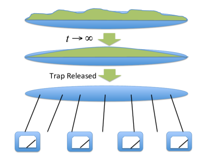
Figure 1: The Lieb Liniger gas is initialized in some nonequilibrium state, allowed to relax for a long time and its correlation functions are measured.

In this work we consider the repulsive Lieb-Liniger model in the limit of infinite interaction strength, Tonks Girardeau limit. We consider the case when the gas was quenched from a non-equilibrium initial state $\left|\Phi_{0}\right\rangle$ - which must be translationally invariant and short ranged correlated - and allowed to relax for a long time thereby establishing a GGE $\left|\Psi\right\rangle=e^{iH_{LL}t}\left|\Phi_{0}\right\rangle$ with $\left|\Psi\right\rangle\left\langle\Psi\right|\cong\rho_{GGE}$ see figure (1). In this regime when the GGE is already established we compute the density density correlation function of the gas and show that at long distances it is of universal form - exponentially decaying $\sim e^{-\kappa x}$. This simple exponential decay is a clear spectroscopic signature of the GGE. In the case when the initial state, and hence the final state, has low entropy per particle key-11 (11) we find that at intermediate distances the density density correlation function has a universal form it is a power law decay $\sim\frac{1}{x^{2}}$, in particular the density density correlation function has three “regions” and looks like the one given in figure (2). Furthermore for any specific initial state with low entropy the exact density density correlation function has a simple form depending only on the the set of points $k_{n}$ such that the energy function vanishes $\varepsilon_{\left\{\alpha\right\}}\left(k\right)\equiv\sum\alpha_{i}k_{n}^{i}=0$. The values $k_{n}$ are readily measurable experimentally through time of flight imaging and are related to rapid changes in the particle distribution function $\rho_{p}\left(k\right)$ discussed below, see figure (3). Thus the density density correlation functions give a finger print signature that the GGE has been established. We also study a generalized case valid when the initial state has long distance correlation functions key-10 (10) and the final sate of the gas is controlled by a generalized GGE. We find that for the case when the initial state has low entropy per particle that the long distance form of the density density correlation function still has a power law form. However the prefactor is a complicated $O\left(1\right)$ non-universal function. We would like to note that the results pertaining to the exponential decay of correlations are based on the assumption that the function $\varepsilon_{\left\{\alpha\right\}}\left(k\right)$ is analytic in the complex plane which would happen for example when the first few conserved quantities dominate the dynamics.

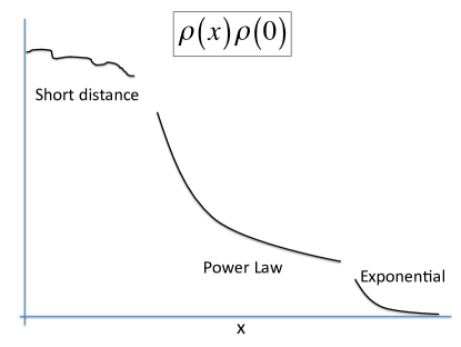
Figure 2: The density density correlation function for the low entropy GGE. There is a complicated short distance region, a power law decay $\sim\frac{1}{x^{2}}$ and an exponential decay at long distances.

The rest of the paper is organized as follows: in Section II we simplify the GGE density matrix by reducing it to a single state $\rho_{GGE}\cong\left|\vec{k}_{0}\right\rangle\left\langle\vec{k}_{0}\right|$; in Section III we present a general from for the density density correlation function, we review the work done in key-3 (3); in Section IV we find the asymptotics of the density density correlation function at long times and large distances for an arbitrary initial state, we find an exponential decay of the correlation function; in Section V we specialize to the case when there is low entropy per particle and find a power law decay of the density density correlation function at intermediate distances; in Section VI based on the results of Section V we present a phenomenological Bosonization theory for the density density correlations for the low entropy GGE state; in Section VII we extend our results to the GGGE and in Section VIII we conclude.

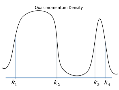
Figure 3: The quasimomentum distribution function $\rho_{p}\left(k\right)$. the points $k_{n}$ are determined when $\rho_{p}\left(k_{n}\right)=\frac{1}{4\pi}$, for the low entropy state these would correspond to rapid changes in the quasiparticle density from $0\leftrightarrow\frac{1}{2\pi}$ see Section V.

II Reduction to a pure state

For the Lieb-Liniger gas it is possible to reduce the GGE density matrix to a pure state. In particular it was shown that the GGE density matrix corresponds to a specific pure state key-1 (1): that is for any local correlation function $\Theta$:

$$tr\left[\Theta\rho_{GGE}\right]=\left\langle\vec{k}_{0}\right|\Theta\left|\vec{k}_{0}\right\rangle$$ (3)

for an appropriately chosen eigenstate of the Lieb Liniger Hamiltonian $\left|\vec{k}_{0}\right\rangle$. Furthermore following the authors of key-1 (1) we are able to specify this pure state $\left|\vec{k}_{0}\right\rangle$. To do so let us denote by $L\rho_{p}\left(k\right)dk$ as the number of particles in the interval $\left[k,k+dk\right]$, $L\rho_{h}\left(k\right)dk$ as the number of holes in the interval $\left[k,k+dk\right]$ and $L\rho_{t}\left(k\right)dk$ as the number of states in the interval $\left[k,k+dk\right]$ so that $\rho_{t}\left(k\right)=\rho_{p}\left(k\right)+\rho_{h}\left(k\right)$. Then the density of particles in k-space corresponding to $\left|\vec{k}_{0}\right\rangle$ is given by the following equations key-1 (1):

$$\begin{array}[]{l}2\pi\rho_{t}\left(k\right)=1+\int_{-\infty}^{\infty}K\left(k,q\right)\rho_{p}\left(k\right)\\ \varepsilon_{\left\{\alpha\right\}}\left(k\right)-\varepsilon_{s}\left(k\right)-\frac{1}{2\pi}\int dqK\left(k,q\right)\ln\left(\varepsilon_{s}\left(q\right)\right)=0\\ \int\rho_{p}\left(k\right)dk=D\end{array}$$ (4)

Here $K\left(k,q\right)=\frac{2c}{c^{2}+\left(k-q\right)^{2}}$ and we have introduced $\frac{\rho_{h}\left(k\right)}{\rho_{p}\left(k\right)}=e^{\varepsilon_{s}\left(k\right)}$, $\varepsilon_{\left\{\alpha\right\}}\left(k\right)=\sum\alpha_{i}k^{i}$ is the energy function of the GGE ensemble and we denote the density of particles by $D$. In the case of the Tonks Girardeau gas this relation between the GGE density matrix and the state $\left|\vec{k}_{0}\right\rangle$ greatly simplifies. In this case density corresponding to the state $\left|k_{0}\right\rangle$ is given by

$$\rho_{t}=\frac{1}{2\pi},\,\varepsilon_{s}\left(k\right)=\varepsilon_{\left\{\alpha\right\}}\left(k\right)\equiv\varepsilon\left(k\right),\,\int\rho_{p}\left(k\right)dk=D$$ (5)

From this it is possible to completely determine the density of particles corresponding to the GGE density matrix, it is given by $\rho_{p}\left(k\right)=\frac{1}{2\pi}\frac{1}{1+e^{\varepsilon\left(k\right)}}$. We note that the density function $\rho_{p}\left(k\right)$ is measurable experimentally.

III Asymptotics of the generating function

As a preliminary step to understand the density density correlation function we would like to study the generating function of density correlations $\Theta_{\beta}\left(x\right)\equiv\exp\left(\beta\int_{0}^{x}b^{\dagger}\left(z\right)b\left(z\right)dz\right)$. It is known key-2 (2) that for a pure state $\left|\vec{k}_{0}\right\rangle$ the expectation value of $\Theta_{\beta}\left(x\right)$ is given by the Fredholm determinant of the sine kernel with respect to the state:

$$\begin{array}[]{l}\left\langle\vec{k}_{0}\right|\Theta_{\beta}\left(x\right)\left|\vec{k}_{0}\right\rangle=\\ =\det\left(I+\frac{e^{\beta}-1}{\pi}\frac{1}{\sqrt{1+e^{\varepsilon\left(k\right)}}}\frac{\sin\left(k-q\right)\frac{x}{2}}{k-q}\frac{1}{\sqrt{1+e^{\varepsilon\left(q\right)}}}\right)\end{array}$$ (6)

The only dependance on $\left|\vec{k}_{0}\right\rangle$ comes from $\varepsilon\left(k\right)\equiv\ln\left(\frac{\rho_{h}\left(k\right)}{\rho_{p}\left(k\right)}\right)$. This Fredholm determinant has been well studied and the large distance asymptotics of this determinant is given by key-3 (3):

$$\left\langle\Theta_{\beta}\left(x\right)\right\rangle=\exp\left(\Delta\left(\nu\right)\right)\det\left(I-A\right)$$ (7)

Here we have introduced the functions $\nu\left(k\right)=\frac{-1}{2\pi i}\ln\left(1+\frac{e^{\beta}-1}{1+e^{\varepsilon\left(k\right)}}\right)$, $\Delta\left(\nu\right)=-\int_{-\infty}^{\infty}ix\nu\left(k\right)dk+\int_{-\infty}^{\infty}\int_{-\infty}^{\infty}\frac{\nu\left(k\right)\nu\left(q\right)}{\left(k-q+i0\right)^{2}}$ , $\alpha\left(k\right)=\exp\left(\int_{-\infty}^{\infty}\frac{\nu\left(q\right)}{q-k}dq\right)$ and $A=A^{-}A^{+}$ . Here $A_{jk}^{-}=\frac{h_{k}^{-}e^{-ixs_{k}^{-}}}{s_{j}^{+}-s_{k}^{-}}$, $A_{jk}^{+}=\frac{h_{k}^{+}e^{ixs_{k}^{+}}}{s_{j}^{-}-s_{k}^{+}}$ with $h_{k}^{\pm}=\frac{\alpha\left(s_{k}^{\pm}\right)^{\mp 2}}{\left(e^{\beta}-1\right)\left(\frac{1}{1+e^{\varepsilon\left(s_{k}^{\pm}\right)}}\right)^{2}e^{\varepsilon\left(s_{k}^{\pm}\right)}\varepsilon^{\prime}\left(s_{k}^{\pm}\right)}$. Here $s_{k}^{\pm}$ refer to the solutions of the equation $1+\frac{e^{\beta}-1}{1+e^{\varepsilon\left(s_{k}^{\pm}\right)}}=0$ with $\pm$ referring to solutions in the upper and lower half plane respectively. This complex formula gives all the density density correlation functions for the GGE. We will study and simplify this formula in the remained of the paper. We note here that the number of solutions $s_{k}^{\pm}$ might be infinite however because of the form of $A_{jk}^{\pm}$ only those near the real axis contribute to the correlation function $\left\langle\Theta_{\beta}\left(x\right)\right\rangle$ so only a finite number of terms matter. Corrections to this result, see Eq. (7) decay faster then any exponential. We note that this result depends on $\varepsilon\left(k\right)$ being analytic in the complex plane, which would happen when the inverse temperatures $\alpha_{i}$ converge fast enough.

IV Density density correlations

We would like to specialize the above formulas, see Eq. (7) to the calculation of density density correlation functions. Since $\left\langle\rho\left(x\right)\rho\left(0\right)\right\rangle=\frac{1}{2}\frac{d^{2}}{d\beta^{2}}\frac{d^{2}}{dx^{2}}\left\langle\Theta_{\beta}\left(x\right)\right\rangle_{\beta=0}$ it is sufficient to expand the above formulas for small $\beta$ upto order $\beta^{2}$. With this in mind its sufficient to simplify $\nu\left(k\right)\cong i\frac{\beta}{2\pi}\frac{1}{1+e^{\varepsilon\left(k\right)}}$, $\Delta\left(\nu\right)\cong-\beta x\int_{-\infty}^{\infty}\frac{1}{1+e^{\varepsilon\left(k\right)}}dk$, and $\alpha\left(k\right)\cong 1$. Furthermore introducing $\tilde{s}_{k}^{\pm}$ as solutions to the equations $\varepsilon\left(\tilde{s}_{k}^{\pm}\right)=\left(2n+1\right)\pi i$ closest to the points $s_{k}^{\pm}$ we have that $h_{k}^{\pm}\cong-\frac{\beta}{\varepsilon^{{}^{\prime}}\left(\tilde{s}_{k}^{\pm}\right)}$ and therefore $A_{jk}^{-}\cong-\frac{\beta}{\varepsilon^{{}^{\prime}}\left(\tilde{s}_{k}^{-}\right)}\frac{e^{-ix\tilde{s}_{k}^{-}}}{\tilde{s}_{j}^{+}-\tilde{s}_{k}^{-}}$, $A_{jk}^{+}\cong-\frac{\beta}{\varepsilon^{\prime}\left(\tilde{s}_{k}^{+}\right)}\frac{e^{ix\tilde{s}_{k}^{+}}}{\tilde{s}_{j}^{-}-\tilde{s}_{k}^{+}}$. We note that the points $\tilde{s}_{k}^{\pm}$ correspond to poles of $\rho_{p}\left(k\right)=\frac{1}{1+e^{\varepsilon\left(k\right)}}$ which are close to solutions of the equation $1+\frac{e^{\beta}-1}{1+e^{\varepsilon\left(k\right)}}=0$ for small $\beta$. Now using $\det\left(I-A\right)\cong 1-tr\left(A\right)$ and combining we get that

$$\left\langle\rho\left(x\right)\rho\left(0\right)\right\rangle=\rho^{2}+\sum_{j,k}\frac{e^{ix\left(\tilde{s}_{j}^{+}-\tilde{s}_{k}^{-}\right)}}{\varepsilon^{\prime}\left(\tilde{s}_{j}^{+}\right)\varepsilon^{{}^{\prime}}\left(\tilde{s}_{k}^{-}\right)}=\rho^{2}+\left|\sum\frac{e^{ix\tilde{s}_{j}^{+}}}{\varepsilon^{\prime}\left(\tilde{s}_{j}^{+}\right)}\right|^{2}$$ (8)

The last equality comes about because of every pole of $\rho_{p}\left(k^{\star}\right)=\rho_{p}\left(k\right)^{\star}$ so a pole at $k$ corresponds to a pole at $k^{\star}$. For very long distances only one of the exponentials dominates and we get that

$$\left\langle\rho\left(x\right)\rho\left(0\right)\right\rangle\cong\rho^{2}+\frac{e^{-2xIm\tilde{s}_{j}^{+}}}{\left|\varepsilon^{{}^{\prime}}\left(\tilde{s}_{j}^{+}\right)\right|^{2}}$$ (9)

As such at long distances the density density correlation function for the Tonks gas after it has reached equilibrium generically has a single exponential decay this result is robust to experimental imperfections. This result compares well with the quench between free bosons and hard core bosons studied in key-13 (13). We would like to note that there are some cases where due to symmetry there are exactly two degenerate minimal $\tilde{s}_{j}^{+}$. This happens for example when $\varepsilon\left(k\right)=\varepsilon\left(-k\right)$. In this case there are two minimal solutions $s_{1}$ and $-s_{1}^{\star}$. Assuming that these are two distinct points, e.g. $s_{1}$ is not purely imaginary we obtain that:

$$\begin{array}[]{l}\left\langle\rho\left(x\right)\rho\left(0\right)\right\rangle\cong\\ \cong\rho^{2}+4\frac{e^{-2xIms_{1}}}{\left|\varepsilon^{\prime}\left(s_{1}\right)\right|^{2}}\sin^{2}\left(xRes_{1}-\ln\left(\frac{\varepsilon^{\prime}\left(s_{1}\right)}{\left|\varepsilon^{\prime}\left(s_{1}\right)\right|}\right)\right)\end{array}$$ (10)

In this case, for a symmetric $\varepsilon\left(k\right)$, we see that there is still an exponential decay but it is now multiplied by $\sin^{2}\left(kx\right)$ with $k=Res_{1}$. This is an excellent spectroscopic tool to determine the GGE as well as to test whether the density of excitations $\rho_{p}\left(k\right)$ is symmetric $\rho_{p}\left(k\right)=\rho_{p}\left(-k\right)$ or not. We note though that the coefficient $Im\tilde{s}_{j}^{+}$ is very hard to determine directly from a measurement of $\rho_{p}\left(k\right)$ because it requires an analytic continuation of the function $\rho_{p}\left(k\right)$ into the upper complex plane, it is measurable from interferometry density density correlation measurement though. Below we shall see that in the case that the initial state has low entropy per particle for intermediate distance scales there is a different universal power law behavior for the correlation functions.

V Low Entropy per Particle

We would like to consider the case where the final state has little entropy per particle, or equivalently its at a low “temperature” key-12 (12). We know that the entropy per unit length is given by $\frac{1}{2\pi}\int dk\left(\frac{1}{1+e^{\varepsilon\left(k\right)}}\ln\left(1+e^{\varepsilon\left(k\right)}\right)+\frac{1}{1+e^{-\varepsilon\left(k\right)}}\ln\left(1+e^{-\varepsilon\left(k\right)}\right)\right)$. We see that this can only be small when either $\frac{1}{1+e^{\varepsilon\left(k\right)}}$ or $\frac{1}{1+e^{-\varepsilon\left(k\right)}}$ are small. From this we see that $\left|\varepsilon\left(k\right)\right|\gg 1$ for most $\varepsilon\left(k\right)$ and that $\tilde{s}_{j}^{+}$ has a large imaginary part except near specific values where $\varepsilon\left(k_{n}\right)=0$. By considering the form of Eq. (8) we see that points with large imaginary values do not contribute so we focus on the case where $\varepsilon\left(k_{n}\right)\cong 0$. Near such points $\varepsilon\left(k\right)\cong\left(k-k_{n}\right)\varepsilon^{\prime}\left(k_{n}\right)$. From this we get that the relevant solutions to $\varepsilon\left(\tilde{s}_{j}^{+}\right)=\left(2m+1\right)\pi i$ are given by $\tilde{s}_{n.m}^{+}\cong k_{n}+i\pi\frac{2m+1}{\varepsilon^{\prime}\left(k_{n}\right)}$ with $m\geq 0$ for $\varepsilon^{\prime}\left(k_{n}\right)>0$ and $\tilde{s}_{n.m}^{+}\cong k_{n}-i\pi\frac{2m+1}{\varepsilon^{\prime}\left(k_{n}\right)}$ with $m\geq 0$ for $\varepsilon^{\prime}\left(k_{n}\right)<0$ see figure (4). Now considering Eq. (8) we see that the sum in the absolute value is given by: $\sum_{m}\frac{e^{ix\tilde{s}_{n.m}^{+}}}{\varepsilon^{\prime}\left(\tilde{s}_{n,m}^{+}\right)}\cong\frac{e^{ik_{n}x}}{\varepsilon^{\prime}\left(k_{n}\right)}\frac{e^{-\pi x/\left|\varepsilon^{\prime}\left(k_{n}\right)\right|}}{1-e^{-2\pi x/\left|\varepsilon^{\prime}\left(k_{n}\right)\right|}}\cong sgn\left(\varepsilon^{\prime}\left(k_{n}\right)\right)\frac{e^{ik_{n}x}}{2\pi x}$. From this we get that for intermediate distances in the low entropy regime

$$\left\langle\rho\left(x\right)\rho\left(0\right)\right\rangle=\rho^{2}+\frac{1}{4\pi^{2}x^{2}}\left|\sum sgn\left(\varepsilon^{\prime}\left(k_{n}\right)\right)e^{ik_{n}x}\right|^{2}$$ (11)

We note that this result is valid when there are many poles near the points $k_{n}$ or alternatively $\left|\varepsilon^{\prime}\left(k_{n}\right)\right|\gg 1$. We see that the density density correlation function in the Tonks regime has universal form. It has a universal $\sim\frac{1}{x^{2}}$ dependance at intermediate distances with the exact prefactor depending only on a few fixed momenta, which may be determined from the conserved quantities $I_{i}$. We note that spectroscopically it is easier to determine the momenta $k_{n}$ from the density function $\rho_{p}\left(k\right)$. The points $k_{n}$ correspond to the points where $\rho_{p}\left(k_{n}\right)=\frac{1}{4\pi}$ which may be easily determined from time of flight imaging. Furthermore these points are highly recognizable since at these points the density function $\rho_{p}\left(k\right)$ has a rapid change $0\leftrightarrow\frac{1}{2\pi}$. This result is universal and as such robust to experimental imperfections. We note that for this section we do not need the analyticity of $\varepsilon\left(k\right)$ in the complex plane just near the real axis (which always happens).

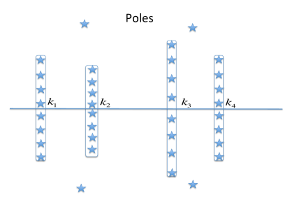
Figure 4: Poles of the particle density function $\rho_{p}\left(k\right)$ in the complex plane. The poles relevant to the low entropy regime near the points $k_{n}$ are circled.

VI Bosonization

Based on our results about the density density correlation function for the low entropy Tonks gas see Eq. (11), we would like to Bosonize our gas. Previous schemes key-4 (4) to bosonize the Lieb Liniger gas were based on considering states with low energy, those near the ground state. Here we would like to bosonize low entropy but potentially high energy states. Following key-4 (4) we introduce $\phi_{l}\left(x\right)$ which counts the number of particles up to the point $x$. Base on key-4 (4) we expect that

$$\rho\left(x\right)=\left[\rho_{0}-\frac{\nabla\phi\left(x\right)}{\pi}\right]\sum e^{ip\left(\rho_{0}-2\phi\left(x\right)\right)}$$ (12)

Here the field $\phi_{l}\left(x\right)$ is rapidly varying and is decomposed into $\phi_{l}\left(x\right)=2\pi\rho_{0}x-2\phi\left(x\right)$ with $\phi$ slowly varying. In our case for low entropy per particle the density of bosons has rapid oscillations at the momenta $k_{n}$ with bosons being added when $\varepsilon^{\prime}\left(k_{n}\right)<0$ and bosons being removed when $\varepsilon^{\prime}\left(k_{n}\right)>0$. The simplest generalization of Eq. (12) that includes oscillations at the momenta $k_{n}$ which gives the correct leading order contributions to the density and is translationally invariant may be written as:

$$\begin{array}[]{l}\rho\left(x\right)=\rho_{0}-\sum_{k_{n}>k_{m}}\frac{1}{\pi\left(N-1\right)}\nabla\phi_{mn}\left(x\right)+\\ +A\sum_{k_{n}>k_{m}}sgn\left(\varepsilon^{\prime}\left(k_{n}\right)\right)sgn\left(\varepsilon^{\prime}\left(k_{m}\right)\right)\times\\ \qquad\times e^{i\left(k_{n}-k_{m}\right)x}e^{-2i\phi_{m,n}\left(x\right)}+h.c.\end{array}$$ (13)

Where $\phi_{mn}$ are slowly varying field and $N$ is the total number of solutions to the equation $\varepsilon\left(k_{n}\right)=0$. We note that we have introduced a total of $\frac{N\left(N-1\right)}{2}$ bosonic fields each corresponding to an appropriate pair of points $k_{n}$ and $k_{m}$ in the case of bosonizing the ground state this would correspond to one field representing the left and right fermi point. Furthermore the simplest action for the fields $\phi_{mn}$ may be written as key-4 (4):

$$S=\frac{1}{2\pi K}\sum_{k_{m}>k_{n}}\int dxd\tau\left(\frac{1}{u}\left(\partial_{\tau}\phi_{mn}\right)^{2}+u\left(\partial_{x}\phi_{mn}\right)^{2}\right)$$ (14)

This corresponds to a sum of independent actions for each bose field. For simplicity we consider the zero temperature limit, it is the one that reproduces the power law decay functions. This allows us to compute the density density correlation function. It is given by:

$$\begin{array}[]{l}\left\langle\rho\left(x,t\right)\rho\left(0,0\right)\right\rangle=\rho^{2}+\frac{NK}{4\pi^{2}}\frac{u^{2}t^{2}+x^{2}}{\left(x^{2}-u^{2}t^{2}\right)^{2}}+\\ \qquad+\frac{A}{\left(x^{2}-u^{2}t^{2}\right)^{K}}\left(\left|\sum sgn\left(\varepsilon^{\prime}\left(k_{n}\right)\right)e^{ik_{n}x}\right|^{2}-N\right)\end{array}$$ (15)

We hypothesize that this form with appropriate $u$ and $K$ is also valid for the Lieb-Liniger gas for intermediate distances when considering a GGE with relatively little entropy per particle. We would like to note that this is only a conjecture and that there are many other ways to bosonize the GGE Lieb liniger gas, for example introduce a $K$ matrix and a $u$ matrix, however this is the simplest translationally invariant way that reduces to known results about bosonizing the ground state of the Lieb Liniger gas and given correct answers for the GGE.

VII Generalized GGE

Recently it has been proposed that for states with long ranged correlation functions the Lieb-Liniger gas does not equilibrate to the GGE but to a generalized version of it, the GGGE key-10 (10). The density matrix for the GGGE ensemble is given by $\rho_{GGGE}=\frac{1}{\tilde{Z}}\exp\left(-\sum\alpha_{i,j,k...}I_{i}I_{j}I_{k}...\right)$. It was shown that for most purposes the GGGE density matrix is equivalent to the diagonal ensemble density matrix key-10 (10) that is $\rho_{GGGE}=\int d\vec{k}f\left(\vec{k}\right)\left|\vec{k}\right\rangle\left\langle\vec{k}\right|$, for $f\left(\vec{k}\right)$ being a positive function of the momenta $\vec{k}$ and $\int d\vec{k}f\left(\vec{k}\right)=1$. Here we would like to show that in the case of initial states with low entropy per particle the density density correlation function still retains its $\sim\frac{1}{x^{2}}$ form. Indeed the density density function is given by:

$$\begin{array}[]{l}\left\langle\rho\left(x\right)\rho\left(0\right)\right\rangle=\int d\vec{k}f\left(\vec{k}\right)\left\langle\vec{k}\right|\rho\left(x\right)\rho\left(0\right)\left|\vec{k}\right\rangle=\\ =\rho^{2}+\frac{1}{x^{2}}\int d\vec{k}f\left(\vec{k}\right)\frac{1}{4\pi^{2}}\left|\sum sgn\left(\varepsilon^{\prime}\left(k_{n}\right)\right)e^{ik_{n}x}\right|^{2}\\ \equiv\rho^{2}+\frac{C\left(x\right)}{x^{2}}\end{array}$$ (16)

Because the integrand in the second line of Eq. (16) is positive and has order one dependence on $x$ we notice that $C\left(x\right)=O\left(1\right)$. We note that this equality strongly depends on the fact that $\left|\sum sgn\left(\varepsilon^{\prime}\left(k_{n}\right)\right)e^{ik_{n}x}\right|^{2}\geq 0$ otherwise averaging could lead to exponentially small results. Therefore upto an order one non-universal order one function the density density correlation function in the GGGE case has a $\sim\frac{1}{x^{2}}$ form for intermediate distances. This is a spectroscopic signature of the GGGE. We note that in principle one could derive this result starting from previous work key-10 (10) however we have a much more direct method.

VIII Conclusions

We have studied the long time dynamics of a Tonks gas. Using the fact that the gas equilibrates to the GGE we were able to find a pure state corresponding to the Tonks gas. We computed exact density density correlation functions for the equilibrated Tonks gas and found them to have exponential decay at long distances. We considered the case where the gas has little entropy per particle and found that at intermediate distances the gas has a power law $\sim\frac{1}{x^{2}}$ density density correlation function. We presented a bosonization hypothesis that allowed us to extend our results to the Lieb Liniger gas with finite interaction strength. In the future it would be interesting to confirm this hypothesis as well as compute other correlation functions. We note that our results provide clear spectroscopic signatures for identifying a GGE using both the density function $\rho_{p}\left(k\right)$ and the density density correlation function $\left\langle\rho\left(x\right)\rho\left(0\right)\right\rangle$. In particular we show that in the low entropy per particle regime the density density correlation has three “regions” which should be easily measurable through interferometry. This result is universal and as such is robust to experimental imperfections.

Acknowledgments: This research was supported by NSF grant DMR 1006684 and Rutgers CMT fellowship.

References

(1) T. Kinoshita, T. Wenger, and D. S. Weiss, Nature
(London) 440, 900 (2006)
(2) S. Hofferberth, I. Lesanovsky, B. Fischer, T.
Schumm, and J. Schmiedmayer, Nature (London) 449, 324 (2007).
(3) N. Gedik, D.-S. Yang, G. Logvenov, I. Bozovic,
and A. H. Zewail, Science 316, 425 (2007).
(4) M. Rigol, V. Dunjko, and M. Olshanii, Nature (London)
452, 854 (2008); M. Rigol, V. Dunjko, V. Yurovsky, and M.
Olshanii, Phys. Rev. Lett. 98, 050405 (2007).
(5) E. H. Lieb and W. Liniger, Phys. Rev. 130, 1605
(1963).
(6)G. Goldstein and N. Andrei, arXiv 1309.7029
(7) We note that entropy per particle is a dimensionless
quantity.
(8) N. A. Slavnov, Theor. Math. Phys. 165,
1262, (2010).