Estimation and Modelling of PCBs Bioaccumulation in the Adriatic Sea Ecosystem

Abstract

Persistent Organic Pollutants represent a global ecological concern due to their ability to accumulate in organisms and to spread species-by-species via feeding connections. In this work we focus on the estimation and simulation of the bioaccumulation dynamics of persistent pollutants in the marine ecosystem, and we apply the approach for reconstructing a model of PCBs bioaccumulation in the Adriatic sea, estimated after an extensive review of trophic and PCBs concentration data on Adriatic species. Our estimations evidence the occurrence of PCBs biomagnification in the Adriatic food web, together with a strong dependence of bioaccumulation on trophic dynamics and external factors like fishing activity.

1 Introduction

Chemical contamination is one of the strongest and most complex abiotic perturbations threatening the stability of marine ecosystems. Constantly, an unrestrained flow of pollutants is released into the seas triggering unpredictable ecological consequences in marine biota, having also cascade effects in the entire ecosystem. The aquatic environment is characterized by multiple contamination pathways making marine organisms particularly prone to bioaccumulation and biomagnification phenomena (defined in Table 1), of which Persistent Organic Pollutants (POPs) are globally recognised as one of the main and worst causes.

Chemically belonging to the same class of POPs, Polychlorinated biphenyl (PCBs) have been for a long time matter of ecotoxicological interest for their property of binding with the fatty tissue of animals and, thus, of spreading through feeding connections amplifying their toxic perturbations species-by-species. As a consequence, feeding links become a critical medium of chemical transport across trophic levels up to the human being (Kelly et al., 2007, Lohmann et al., 2007), which makes the entire marine ecosystem both sink and source of hazardous substances.

Bioaccumulation represents a complex and exhaustive ecotoxicological indicator to evaluate the toxic exposure of living organisms. Its definition (Mackay and Fraser, 2000) includes abiotic and biotic factors (see Table 1), therefore it can vary for the same species surveyed in different environments. Variations may depend on the multiple patterns of uptake and their related concentrations, on the nature of xenobiotics, and on species-specific biological characteristics (lipid content, size, age and etc). The combination of all these aspects with the variety of local environmental and ecological scenarios makes difficult to obtain an all-encompassing model.

In the field of environmental toxicology, prediction-oriented works are still relatively recent. However, over the last decades this area has considerably evolved with advances in models, approaches and indices to assess chemicals fate and effects on species and communities (Van der Oost et al., 2003, Mackay and Fraser, 2000, Arnot and Gobas, 2006, Devillers, 2009, Jørgensen and Bendoricchio, 2001). What makes a model exploitable for predictive purposes is its practical utility and, above all, its ability to reproduce bioaccumulation dynamics in a robust way (Luoma and Rainbow, 2005).

As opposed to regression-based approaches for predicting species bioconcentration or bioaccumulation, mechanistic models (Mackay and Fraser, 2000, Nichols et al., 2009) require specifying and quantifying the different pathways of contaminant uptake and loss. Thus, they provide a more detailed characterization of the bioaccumulation dynamics and can accommodate the use of empirical data so that estimations and predictions are able to reflect measured conditions. In addition, toxicokinetic-toxicodynamic (TKTD) models study the effects of specific molecules at finer scales, including the diffusion within internal compartments (fat tissue, liver, muscle and etc) and the responses at the genetic and cellular levels. It is clear that a large amount of high quality, species-specific, toxicity data are needed to parametrize TKTD models. Therefore, data availability mainly drives the choice of a particular model and its degree of detail. Besides this, simpler models could provide, with less effort, a fair accuracy or predictive power and having more specific models do not necessarily imply better results (Wainwright and Mulligan, 2013, Wania and Mackay, 1999).

In this work, we derive a bioaccumulation model of PCBs in the Adriatic sea, based on one of the most complete trophic studies in this area (Coll et al., 2007). Since PCBs necessarily follow feeding links, we take a mechanistic approach where pathways of contaminant uptake and loss correspond to trophic flows among species and environmental compartments. What makes the Adriatic area of crucial interest from an ecotoxicological point of view is the combination of high environmental variability and biodiversity with several anthropogenic factors, and a peculiar geography and orography.

A number of studies on PCBs concentration in Adriatic species have been carried out during the last decades. Using this literature we have reconstructed a database that includes toxicity data for each considered species (see Table LABEL:tbl:PCBinputdata). However, due to the lack of data for some compartments and their temporal and spatial patchiness, the resulting collection is still incomplete. Hence, we use Linear Inverse Modelling (LIM), a technique typically employed in trophic estimation, to calculate the missing information. In particular, we obtain, as a first result, a static bioaccumulation network model from which we parametrize a Lotka-Volterra ODE system used to analyse the contaminant long-term dynamics through the food web.

With our methodological framework, we show the occurrence of biomagnification in Adriatic species and that bioaccumulation mainly depends on trophic aspects (e.g. diet and fishing).

Table 1: Glossary of ecotoxicological concepts.

Bioconcentration is the net process of chemical adsorption only from water through respiration and dermal surfaces minus eliminations routes (respiration, egestion, growth dilution and metabolic tranformation).

Bioaccumulation refers to the contamination process of an organism resulting from all possible paths of uptake: waterborne (bioconcentration) and dietary sources, net of chemical elimination routes.

Biomagnification is the phenomenon by which predators have higher concentrations than their prey, leading to increasing accumulation of pollutants along increasing trophic levels.

Polychlorinated Biphenyls are synthetic chemical compounds, chemically defined as chlorinated hydrocarbons. They are highly stable molecules with general formula $C_{12}H_{(10-n)}Cl_{n}$ ($n=1,\ldots,10$ number of chlorine atoms), consisting in a group of 209 different congeners. Congeners vary in the degree of chlorination and chlorine position (para, meta and ortho). Higher chlorine contents correspond to higher environmental persistence and lower biodegradability (photolytic, biological and chemical). PCBs are characterized by semi-volatility, low water solubility, low vapour pressure and long-range transport. PCBs have been used in hundreds of commercial and industrial application until their ban in the 80’s, but are still ubiquitous and have been traced even much farther than their application point, like in Arctic regions (Norstrom et al., 1988). Biologically, they are highly noxious for aquatic living organisms for their lipophilicity, i.e. the ability to dissolve in fats and lipids (including oils and non-polar solvents). This gives rise to the phenomena of bioaccumulation and biomagnification in marine food webs, up to the human being (Dewailly et al., 1989).

2 Materials and Methods

2.1 The Adriatic Sea Ecosystem

This study focuses on the Adriatic Sea, a relatively shallow sub-basin of the Mediaterranean Sea (max depth 1250 m) with limited extension (800 km major axis - 200 km minor axis) but characterized by high ecological relevance and environmental variability (Cushman-Roisin et al., 2001), wide diversity of marine species and microbial communities (Coll et al., 2010).

This area is exposed to multiple external forcing mechanisms that combined, lead to adverse effects in the pollution load spilled into the Adriatic ecosystem. The Adriatic region is characterized by high anthropogenic activities (De Lazzari et al., 2004) and river discharge fluctuations.

Geographically, the complex orography of the gulf of Trieste and the Venice lagoon causes a significant penetration and exchange of coastal water into the urban environment. In particular the Po river by crossing a wide industrial and agricultural area, represents the major buoyancy input with an annual mean discharge rate of 1500 $m^{3}\cdot s^{-1}$ accounting for the third of the total riverine freshwater input into the Adriatic Sea Sea (Campanelli et al., 2011). Moreover, the Southern Eastern Adriatic rivers are equally an important potential source of pollutants, being the mainly entrance to the Southern part of the Adriatic Sea (Marini et al., 2010). In relation to this aspects, several surveys conducted in different Adriatic regions report significant concentrations of different xenobiotics detected both in species and environmental compartment (Marini et al., 2012, Bellucci et al., 2002, Horvat et al., 1999, Kannan et al., 2002)

2.2 Input data

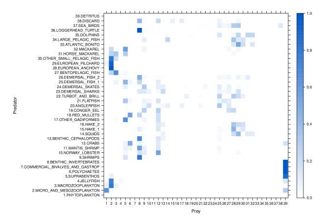
(a) Diet composition matrix

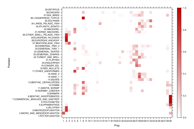
(b) Contaminant uptake from diet matrix

Figure 4: Level plots of the diet composition matrix in the trophic network (a) and of the contaminant uptake rate from diet relative to the PCB bioaccumulation network. Darker cells indicate feeding links where the contribution of the prey in the diet/PCBs concentration of the predator is higher. Diet composition has been taken from Coll et al. (2007), while the uptake rate of a predator $j$ from a prey $i$, $U_{ij}$, is the contaminant flow from $i$ to $j$ scaled by the sum of the inflows of $j$.

In order to define the PCBs bioaccumulation model, we firstly need to estimate the trophic network of Adriatic species. We start from data reported in (Coll et al., 2007), one of the most complete quantitative study of the Northern and Central Adriatic food web in which forty functional groups have been identified to investigate the ecological impact of fishing activity during the decade 1990-2000. In their work the Adriatic trophic model is developed with ECOPATH (Christensen and Walters, 2004), and estimated through a mass balanced approach by using literature and survey data on species abundance. In our model, we follow the same functional group classification as in (Coll et al., 2007), taking the same input data (reported in Table 4) regarding biomass ($B$, measured in $t\cdot km^{-2}$ wet weight organic matter); production/biomass ratio ($P$, i.e. rate of biomass generation, $yr^{-1}$) and consumption/biomass ratio ($Q$, i.e. rate of biomass losses, $yr^{-1}$). Data on fishing activity has also been taken into account, but not reported here. Diet composition is illustrated in Fig. 4 (a) of the supplementary material. Biomass flows are expressed in $t\cdot km^{-2}\cdot yr^{-1}$.

We reviewed a large amount of literature dealing with field analysis of PCBs bioconcentration in marine species of the Adriatic Sea conducted over the last decades. In order to maintain homogeneity with trophic data, we follow some criteria in the selection of the available PCB concentration data. In particular, we collected data sampled in species in North, Central and South Adriatic area during the period 1994-2002, where PCBs concentrations in marine organisms have been determined in edible parts and muscle tissue; and, as usually done in field surveys, we considered the sum of PCBs congeners expressed in $ng\cdot g^{-1}$ wet weight-based. When PCBs values are not available for the same species identified in (Coll et al., 2007), we select concentration data of Adriatic species with the same taxonomic classification. Table LABEL:tbl:PCBinputdata summarizes the PCBs concentration data used in the estimation of the bioaccumulation model for each functional group, together with the corresponding sampled species and literature reference. Details on the sampling period, geographic area, tissue analysed and PCBs congeners detected are summarized in Tab. 6 of the supplement.

2.3 Food web estimation with Linear Inverse Modelling

Following (Ulanowicz, 2004), to describe an ecological network we need its topology (qualitative information), i.e. the nodes representing the relevant groups and the directed edges representing the feeding links; and its flow rates (quantitative information), i.e. for each edge, the rate at which a medium (in our case, biomass or contaminant) is transferred from the source (the prey) to the target (the predator). Generally, flow rates are estimated at some equilibrium conditions, according to which functional groups are mass-balanced, i.e. the inflows must equal the outflows. In addition, each group possesses an internal storage of biomass/bioconcentration affecting the value of flow rates. Food web models need to include also external compartments, used to implement exogenous imports and exports. Externals are not mass-balanced, thus they represent potentially unlimited sources and sinks of medium.

In the following, we denote with $b_{i\xrightarrow[]{}j}$ and $c_{i\xrightarrow[]{}j}$ the flow rate of biomass and contaminant, respectively, from compartment $i$ (the prey) to $j$ (the predator); and the storages $B_{i}$ and $C_{i}$ are used to indicate the biomass and PCBs concentration of $i$, respectively.

One of the most extensively used techniques in reconstructing feeding connections from empirical data is Linear Inverse Modelling (LIM), through which the food web is described as a linear function of its unknown flows. The term inverse indicates that such unknown flows are determined from empirical data, put in the model by means of linear equalities and inequalities (van Oevelen et al., 2010). A LIM problem can be formulated as

$$min\ \ |A\cdot\mathbf{x}-\mathbf{b}|^{2}$$ (2.1)

$$subject\ to\ \ A\cdot\mathbf{x}\simeq\mathbf{b}$$ (2.2)

$$\ E\cdot\mathbf{x}=\mathbf{f}$$ (2.3)

$$\ G\cdot\mathbf{x}\geq\mathbf{h},$$ (2.4)

where $\mathbf{x}$ is the vector of unknown flows; Eq. 2.2 indicates an optional set of equalities that are approximately met (as closest as possible); the strict equalities in Eq. 2.3 are used to model hard constraints, typically to incorporate mass balances and high quality data; and inequalities in 2.4 are used to models soft constraints (e.g. when dealing with low quality data). Among the different methods available for solving a LIM problem, in this work we use the least square method that attempts to minimize the squared difference between the estimates and the data in the approximate equations (see Eq. 2.1), and solutions are accepted up to a fixed tolerance value.

When approximate equalities are excluded and the solution space is not-empty (i.e. when dealing with an under-determined model), a single solution can be picked up that minimizes the sum of squared flows or other global ecosystem properties expressible as linear functions. Alternatively, the solution space can be explored through Monte-Carlo sampling for finding the flows that are most likely under a statistical viewpoint. Then, the mean of the sampled solutions can be taken as a single (valid) solution, as shown in (van Oevelen et al., 2010).

2.4 Adriatic PCBs bioaccumulation model

2.4.1 Conceptual model

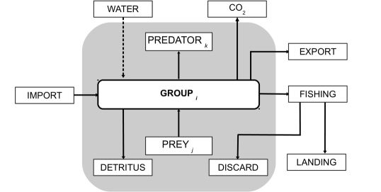
Figure 1: Conceptual model of the Adriatic PCBs bioaccumulation network. Mass-balanced groups are enclosed in the gray box; externals are depicted outside of the box. Generic compartments $i$, $j$, $k$ correspond to any of the mass-balanced groups. Solid arrows indicate combined biomass and contaminant flows between groups. The dashed arrow from the water compartment represents the only contaminant uptake flow which is not mediated by biomass.

Figure 1 illustrates the conceptual model describing the biomass and the PCBs flows between the groups of our network. Given a generic (mass-balanced) group $i$, we consider:

• consumption ($b_{j\xrightarrow[]{}i}$) or contaminant uptake ($c_{j\xrightarrow[]{}i}$) from a prey $j$;

• predation ($b_{i\xrightarrow[]{}k}$) or contaminant losses ($c_{i\xrightarrow[]{}k}$) due to consumption by a predator $k$;

• external inputs of biomass and PCBs from $Import$ ($b_{Import\xrightarrow[]{}i}$ and $c_{Import\xrightarrow[]{}i}$), used to model generic inflows like immigration;

• flows describing contaminant uptake from water ($c_{Water\xrightarrow[]{}i}$), which clearly do not involve a corresponding biomass transfer;

• external outputs to $Export$ ($b_{i\xrightarrow[]{}Export}$ and $c_{i\xrightarrow[]{}Export}$), describing generic outflows like emigration;

• outflows to the $CO_{2}$ compartment ($b_{i\xrightarrow[]{}CO_{2}}$ and $c_{i\xrightarrow[]{}CO_{2}}$), modelling respiration flows and that together with the flows to detritus account for the unassimilated portion of “ingested” food; and

• outflows due to fishing activity, which can be directed to the landings ($b_{i\xrightarrow[]{}Landing}$ and $c_{i\xrightarrow[]{}Landing}$) or to the discards ($b_{i\xrightarrow[]{}Discard}$ and $c_{i\xrightarrow[]{}Discard}$). The latter enters back the biomass cycle and is modelled as a mass-balanced group.

2.4.2 Trophic Network

Table 2 summarizes the linear equalities and inequalities defined for the estimation of biomass flows. The results of the quantification are discussed in Section 3.1 (Fig. 2 (a) gives a graphical illustration of the estimated network and Table 4 reports the numerical results).

Table 2: Linear Inverse Model for the estimation of trophic flows. $b_{i\rightarrow j}$ denotes the biomass flow from group $i$ to group $j$.

Mass balances:$\quad\frac{db_{i}}{dt}=\sum_{j}b_{j\rightarrow i}-\sum_{j}b_{i\rightarrow j}=0$

The difference between inflows and outflows is zero for each functional group $i$; $j$ ranges among groups and externals.

Ingestion1:$\quad I_{i}=\sum_{j}b_{j\rightarrow i}=B_{i}\cdot Q_{i}$

The total ingestion $I_{i}$ of a group $i$, i.e. the sum of all the consumption flows, equals the product between biomass $B_{i}$ and consumption rate $Q_{i}$; $i$ and $j$ are functional groups; for $i$, we exclude detritus and primary producers (phytoplankton).

Unassimilated Food:$\quad b_{i\rightarrow CO2}+b_{i\rightarrow Detritus}=I_{i}\cdot(1-g_{i})$

Respiration flows $b_{i\rightarrow CO2}$ and flows to detritus $b_{i\rightarrow Detritus}$ constitute together a fraction of the total ingestion and accounts for the proportion of food that is not converted into biomass. $g_{i}=\frac{P_{i}}{Q_{i}}$ is the gross food conversion efficiency (Christensen and Walters, 2004).

Respiration-assimilation:$\quad b_{i\rightarrow CO2}\leq I_{i}\cdot g_{i}$

As pointed out in (Coll et al., 2007), the ratio respiration/assimilation has to be lower than one, in order to have realistic estimates.

Diet1:$\quad b_{i\rightarrow j}=I_{j}\cdot DC_{ij}.$

The biomass flow from prey $i$ to predator $j$ is given by the proportion of the total ingestion of $j$ coming from $i$. $DC$ is the diet composition matrix (Fig. 4 (a)).

Non-negativity of flows:$\quad b\geq 0$

1For species with uncertain input biomass and diet data, appropriate inequalities are set.

2.4.3 Bioaccumulation Network

Table 3: Linear Inverse Model for the estimation of PCB concentrations. $c_{i\rightarrow j}$ denotes the contaminant flow from group $i$ to group $j$.

Mass balances:$\quad\frac{dc_{i}}{dt}=\sum_{j}c_{j\rightarrow i}-\sum_{j}c_{i\rightarrow j}=0$

For each group $i\in KINE$, bioconcentrations are estimated under the mass-balance assumption; $j$ ranges among groups and externals.

Concentration data:$\quad C_{i}=PCB_{i}$

These equations incorporate PCB input data ($PCB_{i}$) into the model. Inequalities are used in correspondence of groups with uncertain input PCB concentrations. $i\in KINE\cup INST$.

Uptake from food/losses:$\quad c_{j\rightarrow i}=b_{j\rightarrow i}\cdot C_{j}$

The contaminant flow from $j\in KINE\cup INST$ to $i$ is the product of the corresponding biomass flow $b_{j\rightarrow i}$ and the PCB concentration in $j$. If $i\in KINE$, the equation describes the uptake from food by predator $i$. If instead $i$ is an external, $c_{j\rightarrow i}$ represents a contaminant loss by $j$.

Uptake from generic imports:$\quad c_{import\rightarrow i}=b_{import\rightarrow i}\cdot C_{i}$

The concentration of the biomass imported into group $i\in KINE$) is assumed to be the same as in $i$.

Uptake from environment:$\quad c_{water\rightarrow i}=w_{i}\cdot C_{water}$

$w_{i}$ is the rate of contaminant uptake from water by group $i\in KINE$ and $C_{water}$ is the concentration in water1.

Non-negativity of concentrations:$\quad C_{i}\geq 0$

${}^{1}w_{i}$ cannot directly estimated, since it depends on a non-linear constraint ($w_{i}$ and $C_{water}$ are both unknowns). $c_{water\rightarrow i}$ is instead computed and $w_{i}$ calculated subsequently.

Following (Hendriks et al., 2001, Laender et al., 2009), our bioaccumulation model distinguishes between two kinds of functional groups:

$i\in INST$:

compartments modelling small particles that are assumed to be in instant equilibrium with the water phase, like detritus and planktonic groups. For such groups, contaminant concentration is computed as:

$$C_{i}=C_{water}\cdot OC_{i}\cdot K_{OC}$$

where $C_{i}$ is the concentration of $i$ and $OC_{i}$ is its organic carbon fraction; $C_{water}$ ($\mu g/L$) is the unknown concentration in water and $K_{OC}=k_{OC/OW}\cdot K_{OW}$ is the organic carbon-water partition ratio, calculated as a function of $K_{OW}$, the octanol-water partition ratio of the contaminant. $K_{OW}$ is a measure of how a compound is hydrophilic or hydrophobic, and in this case its value depends on the particular PCB congener considered. Since we consider the sum of congeners, we set $K_{OW}=10^{6}$, given that the $LogK_{OW}$ of PCBs varies between 5 and 7, as reported in (Walters et al., 2011). The other parameters have been taken from (Laender et al., 2009): $OC_{i}=0.028$ and $k_{OC/OW}=0.41$.

$i\in KINE$:

compartments whose concentration depends on the amount of contaminant exchanged through biomass flows, and are estimated as in Table 3. This option applies to groups where contaminant uptake and losses resulting from absorption, ingestion, egestion, excretion and growth cannot be neglected (Hendriks et al., 2001).

We formulate a linear inverse model (Table 3) where PCB concentrations $C_{i}$ are the unknowns to estimate, differently from the trophic model where biomass flows are the unknown variables. Contaminant flows are expressed in $ng\cdot g^{-1}\cdot t\cdot km^{-2}\cdot y^{-1}$. In Section 3.1 we illustrate the estimated PCB bioaccumulation network and we evaluate biomagnification phenomena on the species of the Adriatic ecosystem. Numerical results are reported in Table 6.

2.5 Derivation of ODE Model

Recalling that PCB diffusion follows the same paths as biomass flows determined by prey-predator relationships, we define a dynamic bioaccumulation model on top of a multi-species Lotka-Volterra system used to describe the temporal changes in species biomass. In its general form, the system is formulated as:

$$\dot{B}_{i}(t)=B_{i}(t)\left(g_{i}-\sum_{j}A_{ij}B_{j}(t)\right)$$ (2.5)

where $B_{i}(t)$ is the biomass of species $i$ at time $t$; $g_{i}$ is the intrinsic growth rate of $i$; and $A$ is the interaction matrix describing inter-specific effects. In particular $A_{ij}$ describes the predation effect of species $j$ on species $i$. Although there are several possible ways to derive population-dynamics parameters from a food web model (Palamara et al., 2011), here we follow quite a standard approach:

• $B_{i}(0)=B_{i}$, initial biomass values are those in the static food web estimated with LIM;

• $g_{i}=\dfrac{\sum_{j}b_{j\rightarrow i}-\sum_{j}b_{i\rightarrow j}}{B_{i}(0)}$, with $j$ ranging among the external groups: the growth rate of $i$ is the sum of exogenous inflows and outflow, over the estimated biomass of $i$;

• $A_{ij}=\dfrac{b_{i\rightarrow j}-b_{j\rightarrow i}}{B_{i}(0)\cdot B_{j}(0)}$, the interaction rate between prey $i$ and predator $j$ is calculated as the net flow going from $i$ to $j$ divided by the estimated biomasses of $i$ and $j$.

Additionally, we can define the biomass flow rate from group $i$ to $j$ at time $t$, $b_{i\rightarrow j}(t)$, which is non-linear with respect to the biomasses of $i$ and $j$, as:

$$b_{i\rightarrow j}(t)=\dfrac{b_{i\rightarrow j}}{B_{i}(0)\cdot B_{j}(0)}\cdot B_{i}(t)\cdot B_{j}(t)$$

in a way that Eq. 2.5 can be rewritten as:

$$\dot{B}_{i}(t)=g_{i}\cdot B_{i}(t)+\sum_{j}b_{j\rightarrow i}(t)-\sum_{j}b_{i\rightarrow j}(t)$$

Therefore, the dynamics of the contaminant concentration in species $i$, $C_{i}(t)$, is given by the net sum of contaminant flows, over the biomass of $i$:

$$\dot{C}_{i}(t)=w_{i}\cdot C_{water}+\\ \dfrac{g_{i}\cdot B_{i}(t)\cdot C_{i}(t)+\sum_{j}b_{j\rightarrow i}(t)\cdot C_{j}(t)-\sum_{j}b_{i\rightarrow j}(t)\cdot C_{i}(t)}{B_{i}(t)}$$ (2.6)

where $C_{water}$ is the concentration in water (assumed constant) and $w_{i}$ is the uptake rate from water by group $i$. As done for the biomass equations, the initial concentrations correspond to those estimated in the static bioaccumulation network: $C_{i}(0)=C_{i}$, for each group $i$.

Finally, expanding the interaction terms, Eq. 2.6 is equivalent to the following:

$$\dot{C}_{i}(t)=w_{i}\cdot C_{water}+g_{i}\cdot C_{i}(t)+\sum_{j}\left(\dfrac{b_{j\rightarrow i}}{B_{i}(0)\cdot B_{j}(0)}\cdot B_{j}(t)\cdot C_{j}(t)\right)\\ -\sum_{j}\left(\dfrac{b_{i\rightarrow j}}{B_{i}(0)\cdot B_{j}(0)}\cdot B_{j}(t)\cdot C_{i}(t)\right)$$ (2.7)

In the remainder of the paper, we will focus on the temporal changes in bioconcentrations independently of the biomass variations, thus assuming constant species biomass ($B_{i}(t)=B_{i}(0),\forall t$), which gives the following system of linear differential equations:

$$\dot{C}_{i}(t)=w_{i}\cdot C_{water}+g_{i}\cdot C_{i}(t)+\sum_{j}\left(\dfrac{b_{j\rightarrow i}\cdot C_{j}(t)-b_{i\rightarrow j}\cdot C_{i}(t)}{B_{i}(0)}\right)$$ (2.8)

Note that this simplification does not change the quantitative dynamics of the model, because biomasses have been estimated under mass-balance conditions.

3 Results and Discussion

3.1 Estimated Trophic and Contaminant Network

The estimated trophic and contaminant flows of the Adriatic Sea model are depicted in Figure 2, and the corresponding numerical results are reported in Table 4 for the biomass network, and in Table 6 for the PCBs bioaccumulation network. Estimating the trophic network with LIM required to take an approximate solution (with error tolerance $\leq 10^{-8}$) because the large amount of input trophic data taken from (Coll et al., 2007) (reported in Table 4) generates a high number of constraints and in turn an empty solution space. On the other hand, the partial availability of PCBs bioconcentration data produces an under-determined problem (i.e. many possible solutions), solved in this case through Markov Chain Monte Carlo (MCMC) sampling (5000 iterations) of the solution space.

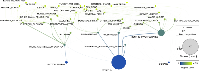
(a) Biomass network

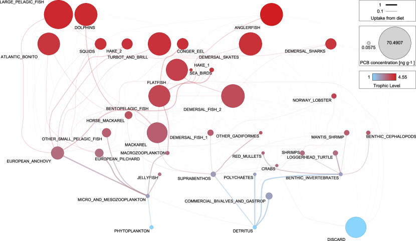
(b) Bioaccumulation network

Figure 2: Estimated Adriatic trophic (a) and PCB bioaccumulation (b) networks. Nodes represent functional groups whose size is proportional to the biomass content (a) or PCB bioconcentration (b). Edges represent feeding connection and their thickness indicates the contribution of the source node in the diet of the target node (a), or in the uptake of contaminant from food in the case of bioaccumulation network (b). Flows to detritus and to fishing discards are not shown.

Trophic Network Analysis

The analysis of the biomass network shows that species at lower trophic levels are the most prominent in terms of internal and exchanged biomass and that biomass content and trophic level are negatively correlated, as visible in Fig. 2 (a). The only exception is the Discard group, which accounts for the discarded catches that enter back the biomass cycle. Discard is considered in this model as a detritus, and thus has associated a trophic level (TL) of 1. However, it clearly possesses a much lower biomass than the natural detritus (group Detritus) and primary producers (group Phytoplankton). We report that our quantitative estimations agree with the original work by Coll et al., which allows us to validate our trophic model.

PCBs Bioaccumulation Analysis

On the other hand, PCBs bioaccumulation values tend to increase at higher trophic levels, thus a phenomenon of biomagnification is clearly detectable, as one can observe in the network plot (Fig. 2 (b)).We also evince that functional groups with high concentrations have associated low biomass values.

We indeed register the most prominent PCBs values in top predators: Large Pelagic Fish (TL = 4.343, PCB = 70.491), Demersal skates (TL = 4.154, PCB = 54.833), Turbot and brill (TL = 4.152, PCB = 54.746), Dolphins (TL=4.302, PCB=54.048), Anglerfish (TL = 4.553, PCB = 53.808), and Atlantic bonito (TL = 4.087, PCB = 52.704). In particular, Large Pelagic Fish (Tuna and Swordfish) shows by far the highest PCBs bioaccumulation, which can be explained by the concentration in groups composing its diet (mainly European Anchovy and Squids).

Anyway, by the nature of the LIM approach, we note that input concentration data strongly influence estimated values. Specifically, low upper bounds on PCBs values limit the output concentrations in some top predators (Squids, Hake 2 and Demersal Sharks). On the contrary, setting high or infinite upper bounds results in large bioaccumulation values also for groups at TL=3, like in Demersal fish 2, Flatfish, Bentopelagic fish and Mackarel. Naturally, having employed a stochastic search algorithm, the concentration variables with less constraints typically have a higher variability (see standard deviation $\sigma$ in Table 6).

Fishing activity and overexploitation represent a biomass loss, and therefore can also affect the patterns of PCBs diffusion in the ecosystem. Bioaccumulation results from the continuous uptake of pollutants over the years. Thus, fishing activity can ideally interrupt the bioaccumulation process by increasing the mortality rate of a species, even if overexploitation is not clearly an ecologically sustainable solution (Coll et al., 2008). In our model, relatively low PCBs values can be detected in correspondence of exploited species (i.e. with fishing rates exceeding biomass). For instance, Crabs, Other gadiformes and Red mullets show concentrations substantially lower ($<1\ ng\cdot g^{-1}$) than those in species belonging to the same TL, but not affected by fishing pressure. A similar phenomenon is observable in Conger eel where, albeit with a wide PCBs input range, the estimated bioaccumulation value stands close to the lower bound. This is even more evident by looking at the variations in PCBs bioaccumulation between groups describing the same species but subject to different fishing pressures, like between Hake 1 ($<40\ cm$, vulnerable to fishing, PCB=3.852) and Hake 2 ($>40\ cm$, not vulnerable, PCB=21.658); or between Demersal fish 1 (overexploited, PCB=8.159) and Demersal fish 2 (PCB=55.424).

Differently from natural detritus, fishing discards are characterized by a significant PCBs concentration. This has to be attributed mainly to its low total biomass, combined with its species composition, that contributes to a considerable total inflow of contaminant as detailed in Table 6 (column $Dis$).

Finally, with our bioaccumulation model we are also able to estimate PCBs concentration in the landing fraction of biomass exported by fishing. This is simply computed as the sum of contaminant outflows to the landings over the sum of biomass exported to the same compartment: $\dfrac{\sum_{i}c_{i\rightarrow Land}}{\sum_{i}b_{i\rightarrow Land}}$. The mean concentration value in landings equals to 18.17 $ng\cdot g^{-1}$. This kind of analysis could provide an effective indicator of the chemical pollution in species of commercial interest.

3.2 ODE bioaccumulation model

We evaluate the long-term bioaccumulation dynamics in the Adriatic food web by simulating the ODE model at Eq. 2.8 for a period of 4 years with a time step of 1 month. We just report the sum of PCBs concentrations (Figure 3) under default initial conditions (derived from network estimations) and under random perturbations of the input concentrations (100 uniformly distributed values for each species).

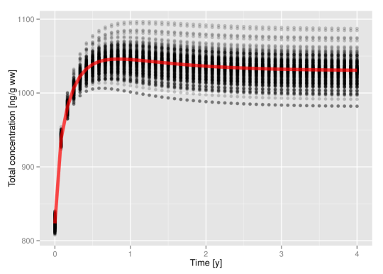
Figure 3: Temporal evolution of total PCBs concentrations, simulated through the dynamic ODE model over a period of 4 years and time step of 1 month (red line). Shaded dots indicate the results obtained after 100 random perturbations of the initial concentration, for each species.

We notice that the qualitative dynamics of the system are robust with respect to changes in the initial conditions. At the same time, the model is able to reproduce the quantitative impact of perturbations in PCBs concentrations, which tends to be amplified over the time. The initial steep increase in total bioaccumulation is attributable to the fact that groups in rapid equilibrium with the water compartment ($INST$ class) are not mass-balanced in the bioaccumulation network. This implies that the initial ODE state is far from equilibrium conditions, that are in any case practically reached within the first 2 years, and despite of random perturbations.

3.3 Implementation

Our bioaccumulation model has been implemented in R. The LIM package (van Oevelen et al., 2010) was used to estimate trophic and bioaccumulation networks. This package has been preferred to the ECOPATH software (Christensen and Walters, 2004), a de facto standard in trophic estimation and analysis, because LIM supports custom models and equations and is general enough to describe multiple flow currencies (both biomass and PCBs), a crucial feature in our study.

The calculation of trophic levels ($TL$ and $OI$) has been performed with the R package NetIndices (Kones et al., 2009), and we used the package FME (Soetaert and Petzoldt, 2010) for ODE simulations. Network plots have been generated with Graphviz (Ellson et al., 2002). Source code is available upon request to authors.

4 Conclusions

The main contribution of this study is the combination of computational and network analysis tools in order to investigate the bioaccumulation of Persistent Organic Pollutants in marine food webs. We consider the case study of PCBs bioaccumulation in the Adriatic sea, providing a state of the art review on PCBs concentration data for the Adriatic food web and the first network level reconstruction, which allows us to evaluate the occurrence of biomagnification through trophic levels. In this context, Linear Inverse Modelling provides effective means to formulate our estimation problem and to deal with incomplete and uncertain data, which we quantified also with a stochastic search of the admissible contaminant flow values.

The derived dynamic ODEs simulated under random perturbation of the initial PCBs concentrations, show robust qualitative dynamics which sets the ground for a deeper study on the temporal bioaccumulation dynamics in the Adriatic ecosystem.

Appendix A Supplementary Material

Table 4: Input PCBs bioconcentration data ($ng\cdot g^{-1}$) by functional group and corresponding references. In order to account for multiple data, we derive concentration ranges instead of single values.

Id	Group	$\sum$PCB min	$\sum$PCB max	Species and References
1	Phytoplankton
2	Micro and mesozoop.
3	Macrozooplankton
4	Jellyfish
5	Suprabenthos
6	Polychaetes
7	Commercial bivalves	1.24	20.29	M. galloprovincialis (Perugini et al., 2004); M. galloprovincialis, C. gallina (Bayarri et al., 2001); C. gallina, A. tubercolata, E. siliqua, M. galloprovincialis (Marcotrigiano and Storelli, 2003)
8	Benthic Invertebrates
9	Shrimps	0.346	11.61	P. longirostris, A. antennatus (Marcotrigiano and Storelli, 2003); A. antennatus, P. longirostris, P. martia (Storelli et al., 2003)
10	Norway lobster	0.2	10.63	N. norvegicus (Bayarri et al., 2001, Perugini et al., 2004, Storelli et al., 2003)
11	Mantis shrimp	2.64	11.61	S. mantis (Marcotrigiano and Storelli, 2003)
12	Crabs
13	Benthic cephalopods	0.31	6.7	T. sagittatus, S. officinalis (Perugini et al., 2004); O. salutii (Marcotrigiano and Storelli, 2003)
14	Squids	9.53	37.7	L. vulgaris (bayarri2001pcdds); I. coindetii (Marcotrigiano and Storelli, 2003)
15	Hake 1	3.183	31.93	M. merluccius (Storelli et al., 2003, Marcotrigiano and Storelli, 2003)
16	Hake 2
17	Other gadiformes
18	Red mullets
19	Conger eel	22.424	104	C. conger (Storelli et al., 2003, 2007a)
20	Anglerfish	0.2		L. boudegassa (Storelli et al., 2003)
21	Flatfish
22	Turbot and brill
23	Demersal sharks	2	42	C. granolousus, S. blainvillei (Storelli and Marcotrigiano, 2001);
24	Demersal skates	0.45		R. miraletus, R. clavata, R. oxyrhincus (Storelli et al., 2003);
25	Demersal fish 1	6.687		S. flexuosa, H. dactyloptereus (Storelli et al., 2003)
26	Demersal fish 2	6.687
27	Bentopelagic fish	6.687
28	European Anchovy	1.22	62.7	E. encrasicolus (Perugini et al., 2004, Bayarri et al., 2001)
29	European Pilchard	5.327	26.25	S. pilchardus (Perugini et al., 2004, Storelli et al., 2003)
30	Small Pelagic Fish	4.54	31.9	S. aurita (Marcotrigiano and Storelli, 2003); S. maris, A. rochei (Storelli et al., 2003)
31	Horse Mackarel	6.761		T. trachurus (Storelli et al., 2003)
32	Mackarel	0.95	80.6	S. scombrus (Perugini et al., 2004, Bayarri et al., 2001)
33	Atlantic bonito
34	Large Pelagic Fish
35	Dolphins
36	Loggerhead turtle	0.63	23.49	C. caretta (Storelli et al., 2007b, Corsolini et al., 2000)
37	Sea birds
38	Discard
39	Detritus

Table 5: Input and estimated data for the trophic newtork. Input data are: $B_{\text{in}}$, input biomass ($t\cdot km^{-2}$); $P$, production rate ($yr^{-1}$); $Q$, consumption rate ($yr^{-1}$). $B_{\text{out}}$ ($t\cdot km^{-2}$) is the estimated biomass; $F$ is the biomass exports due to fishing ($t\cdot km^{-2}\cdot yr^{-1}$), and $Dis$ the fraction discarded. Trophic level analysis is summarized in $OI$, omnivory index; and $TL$, trophic level.

Id	Group	$B_{\text{in}}$	$P$	$Q$	$B_{\text{out}}$	$F$	$Dis$	$OI$	$TL$
1	Phytoplankton	16.658	69.03		16.658	0	0	0	1
2	Micro and mesozooplankton	9.512	30.43	49.87	9.512	0	0	0.053	2.053
3	Macrozooplankton	0.54	21.28	53.14	0.54	0	0	0.210	3.047
4	Jellyfish	4	14.6	50.48	4	0	0	0.228	2.884
5	Suprabenthos	1.01	8.4	54.36	1.01	0	0	0.100	2.105
6	Polychaetes	9.984	1.9	11.53	9.984	0	0	0	2
7	Commercial bivalves and gastrop	0.043	1.06	3.13	0.043	0.035	0	0	2
8	Benthic Invertebrates	79.763	1.06	3.13	79.763	0.328	0.328	0	2
9	Shrimps		3.21	7.2	0.68	0.033	0.017	0.022	3.018
10	Norway lobster	0.018	1.25	4.56	0.018	0.037	0	0.212	3.771
11	Mantis shrimp	0.015	1.5	4.56	0.015	0.072	0	0.226	3.307
12	Crabs	0.009	2.44	4.73	0.009	0.179	0.177	0.352	2.998
13	Benthic cephalopods	0.068	2.96	5.3	0.068	0.156	0.002	0.281	3.307
14	Squids	0.02	3.11	26.47	0.02	0.041	0	0.040	4.140
15	Hake 1	0.06	1	4.24	0.06	0.183	0.07	0.132	3.996
16	Hake 2		0.5	1.85	0.56	0	0	0.027	4.114
17	Other gadiformes	0.029	1.59	4.37	0.029	0.108	0.083	0.202	3.369
18	Red mullets	0.025	1.9	8.02	0.025	0.112	0	0.153	3.190
19	Conger eel	0.005	1.92	6.45	0.005	0.008	0.008	0.078	4.156
20	Anglerfish	0.006	1.04	4.58	0.006	0.007	0	0.095	4.553
21	Flatfish	0.009	1.43	9.83	0.009	0.04	0	0.451	3.886
22	Turbot and brill		1.43	5.34	0.04	0.016	0	0.046	4.152
23	Demersal sharks	0.018	0.63	4.47	0.018	0.008	0	0.260	4.086
24	Demersal skates	0.003	1.11	7.08	0.003	0.002	0	0.252	4.154
25	Demersal fish 1	0.056	2.4	7.68	0.056	0.106	0.051	0.238	3.315
26	Demersal fish 2		2.4	5.68	0.24	0.017	0.001	0.495	3.619
27	Bentopelagic fish		1.07	7.99	1.2	0.002	0	0.212	3.731
28	European Anchovy	1.019 - 6.611	0.87	11.02	1.497	0.501	0.005	0	3.053
29	European Pilchard	2.985 - 7.803	0.75	9.19	2.985	0.406	0.042	0.082	2.968
30	Other small Pelagic Fish	0.413 - 1.517	1.1	11.29	1.517	0.013	0.001	0.158	3.251
31	Horse Mackarel	0.659 - 2.455	0.99	7.57	2.455	0.022	0.002	0.243	3.493
32	Mackarel	0.452 - 1.683	0.99	6.09	1.683	0.025	0.008	0.217	3.319
33	Atlantic bonito	0.3	0.39	4.54	0.3	0.018	0	0.021	4.087
34	Large Pelagic Fish	0.138	0.37	1.99	0.138	0.026	0	0.219	4.343
35	Dolphins	0.012	0.08	11.01	0.012	0.0001	0.0001	0.076	4.302
36	Loggerhead turtle	0.032	0.17	2.54	0.032	0.004	0.004	0.010	3.010
37	Sea birds	0.001	4.61	69.34	0.001	0	0	0.597	3.899
38	Discard	0.733			0.733	0	0	0	1
39	Detritus	200			200	0	0	0	1

Table 6: PCBs concentrations ($\sum$PCB${}_{\text{est}}$, $ng\cdot g^{-1}$) and standard deviations ($\sigma$, $ng\cdot g^{-1}$) obtained with MCMC-based sampling. $F$ ($t\cdot ng\cdot y^{-1}\cdot km^{-2}$) indicates PCBs outflows due to fishing, and $Dis$ the fraction discarded.

Id	Group	$\sum$PCB${}_{\text{est}}$	$\sigma$	$F$	$Dis$
1	Phytoplankton	2.247	0.955	0	0
2	Micro and mesozooplankton	2.247	0.955	0	0
3	Macrozooplankton	2.247	0.955	0	0
4	Jellyfish	0.843	0.353	0	0
5	Suprabenthos	5.952	3.247	0	0
6	Polychaetes	0.348	0.200	0	0
7	Commercial bivalves and gastrop	10.502	5.369	0.368	0
8	Benthic Invertebrates	2.120	0.846	0.696	0.696
9	Shrimps	4.746	2.752	0.157	0.081
10	Norway lobster	5.542	3.115	0.205	0
11	Mantis shrimp	6.103	3.228	0.439	0
12	Crabs	0.058	0.039	0.010	0.010
13	Benthic cephalopods	3.198	1.770	0.499	0.006
14	Squids	23.289	8.172	0.955	0
15	Hake 1	3.852	0.617	0.705	0.270
16	Hake 2	21.658	5.950	0	0
17	Other gadiformes	0.567	0.285	0.061	0.047
18	Red mullets	0.385	0.262	0.043	0
19	Conger eel	22.879	0.443	0.183	0.183
20	Anglerfish	53.808	29.234	0.377	0
21	Flatfish	51.436	30.137	2.057	0
22	Turbot and brill	54.746	28.303	0.876	0
23	Demersal sharks	21.840	11.571	0.175	0
24	Demersal skates	54.833	29.337	0.110	0
25	Demersal fish 1	8.159	1.132	0.865	0.416
26	Demersal fish 2	55.424	28.667	0.942	0.055
27	Bentopelagic fish	51.324	28.892	0.103	0
28	European Anchovy	27.104	18.170	13.579	0.136
29	European Pilchard	14.969	6.234	6.077	0.629
30	Other small Pelagic Fish	16.533	8.180	0.215	0.017
31	Horse Mackarel	12.496	1.171	0.275	0.025
32	Mackarel	47.960	21.422	1.199	0.384
33	Atlantic bonito	52.704	29.504	0.949	0
34	Large Pelagic Fish	70.491	20.461	1.833	0
35	Dolphins	54.048	29.286	0.005	0.005
36	Loggerhead turtle	5.478	4.412	0.022	0.022
37	Sea birds	0.161	0.058	0	0
38	Discard	49.005	0.840	0	0
39	Detritus	2.247	0.955	0	0

Table 7: Summary of the studies considered for the parametrization of the PCBs bioaccumulation model. We report reference; period and area of analysis; species considered; kind of tissue sampled; units of measurement; and PCBs congeners detected.

Reference	Period	Area	Species	Tissue	Units	PCBs congeners
(Perugini et al., 2004)	2002	Center	M. galloprovincialis, N. norvegicus, M. barbatus, S. officinalis, E. flying squid, E. encrasicholus, S. pilchardus, S.r scombrus	edible	ng/g ww	28, 52, 101, 118, 138, 153, 180
(Marcotrigiano and Storelli, 2003)		Adriatic, Ionian Sea	M. Merluccius, M. poutassou, P. blennoides, S. smaris, S. pilchardus, E. encrasicholus, L. caudatus, H. dactylopterus, L. budegassa, T. trachurus, A. rochei, Raje spp, P. glauca, S. acanthias, S. blainvillei, S. canicula, G. melastomus, C. gallina, A. tubercolata, E. siliqua, M. galloprovincialis, O. salutii, I. coindeti, S. mantis, P. longirostris, A. antennatus	muscle	ng/g ww	8, 20, 28, 35, 52, 60, 77, 101, 105, 118, 126, 138, 153, 156, 169, 180, 209
(Bayarri et al., 2001)	1997-1998	North, Center, South	L. vulgaris, M. galloprovincialis, N. norvegicus, M. barbatus, C. gallina	edible	ng/g ww	28, 52, 101, 118, 138, 153, 180, 138, 163
(Storelli et al., 2003)	2001	South	C. conger, H. dactylopterus, L. boudegassa, M. barbatus, S. flexuosa, P. blennoides, P. erythrinus, R. clavata, R. oxyrinchus, R. miraletus, S. pilchardus, M. merluccius, S. aurita, S. scombrus, T. trachurus, A. antennatus, N. norvegicus, P. longirostris, P. martia	muscle	pg/g ww	60, 77, 101, 105, 118, 126, 138, 153, 156, 169, 180, 209
(Storelli et al., 2007a)		South	A. anguilla	muscle	ng/g ww	52, 70, 77, 101, 105, 118, 126, 138, 153, 180
(Storelli and Marcotrigiano, 2001)	1999	South	C. granulosus, S. blainvillei	muscle	ng/g ww	8, 20, 28, 35, 52, 60, 77, 101, 105, 118, 126, 138, 153, 156, 169, 180, 209
(Storelli et al., 2007b)		Adriatic, Ionian Sea	C. caretta	muscle	ng/g ww	8, 20, 28, 35, 52, 60, 77, 101, 105, 118, 126, 138, 153, 156, 169, 180, 209
(Corsolini et al., 2000)	1994	Adriatic, Baltic, Northern Sea	C. caretta	muscle	ng/g ww	153, 137, 138, 180, 170, 194, 60, 118, 105, 156, 189, 77, 126, 169

References

- Arnot and Gobas (2006) Arnot, J.A., Gobas, F.A.. A review of bioconcentration factor (BCF) and bioaccumulation factor (BAF) assessments for organic chemicals in aquatic organisms. Environmental Reviews 2006;14(4):257–297.
- Bayarri et al. (2001) Bayarri, S., Baldassarri, L.T., Iacovella, N., Ferrara, F., Domenico, A.d.. PCDDs, PCDFs, PCBs and DDE in edible marine species from the Adriatic Sea. Chemosphere 2001;43(4):601–610.
- Bellucci et al. (2002) Bellucci, L.G., Frignani, M., Paolucci, D., Ravanelli, M.. Distribution of heavy metals in sediments of the Venice Lagoon: the role of the industrial area. Science of the Total Environment 2002;295(1):35–49.
- Campanelli et al. (2011) Campanelli, A., Grilli, F., Paschini, E., Marini, M.. The influence of an exceptional Po River flood on the physical and chemical oceanographic properties of the Adriatic Sea. Dynamics of Atmospheres and Oceans 2011;52(1):284–297.
- Christensen and Walters (2004) Christensen, V., Walters, C.. Ecopath with Ecosim: methods, capabilities and limitations. Ecological modelling 2004;172(2):109–139.
- Coll et al. (2008) Coll, M., Libralato, S., Tudela, S., Palomera, I., Pranovi, F.. Ecosystem overfishing in the ocean. PLoS one 2008;3(12):e3881.
- Coll et al. (2010) Coll, M., Piroddi, C., Steenbeek, J., Kaschner, K., Lasram, F.B.R., Aguzzi, J., Ballesteros, E., Bianchi, C.N., Corbera, J., Dailianis, T., et al. The biodiversity of the Mediterranean Sea: estimates, patterns, and threats. PloS one 2010;5(8):e11842.
- Coll et al. (2007) Coll, M., Santojanni, A., Palomera, I., Tudela, S., Arneri, E.. An ecological model of the Northern and Central Adriatic Sea: analysis of ecosystem structure and fishing impacts. Journal of Marine Systems 2007;67(1):119–154.
- Corsolini et al. (2000) Corsolini, S., Aurigi, S., Focardi, S.. Presence of Polychlorobiphenyls (PCBs) and Coplanar Congeners in the Tissues of the Mediterranean Loggerhead Turtle Caretta caretta. Marine Pollution Bulletin 2000;40(11):952–960.
- Cushman-Roisin et al. (2001) Cushman-Roisin, B., Gacic, M., Poulain, P.M., Artegiani, A.. Physical oceanography of the Adriatic Sea. Kluwer Academic Publishers, 2001.
- De Lazzari et al. (2004) De Lazzari, A., Rampazzo, G., Pavoni, B.. Geochemistry of sediments in the Northern and Central Adriatic Sea. Estuarine, Coastal and Shelf Science 2004;59(3):429–440.
- Devillers (2009) Devillers, J.. Ecotoxicology modeling. volume 2. Springer, 2009.
- Dewailly et al. (1989) Dewailly, E., Nantel, A., Weber, J.P., Meyer, F.. High levels of PCBs in breast milk of Inuit women from Arctic Quebec. Bulletin of Environmental Contamination and Toxicology 1989;43(5):641–646.
- Ellson et al. (2002) Ellson, J., Gansner, E., Koutsofios, L., North, S.C., Woodhull, G.. Graphviz—open source graph drawing tools. In: Graph Drawing. Springer; 2002. p. 483–484.
- Hendriks et al. (2001) Hendriks, A.J., van der Linde, A., Cornelissen, G., Sijm, D.T.. The power of size. 1. Rate constants and equilibrium ratios for accumulation of organic substances related to octanol-water partition ratio and species weight. Environmental toxicology and chemistry 2001;20(7):1399–1420.
- Horvat et al. (1999) Horvat, M., Covelli, S., Faganeli, J., Logar, M., Mandić, V., Rajar, R., Širca, A., Žagar, D.. Mercury in contaminated coastal environments; a case study: the Gulf of Trieste. Science of the Total Environment 1999;237:43–56.
- Jørgensen and Bendoricchio (2001) Jørgensen, S.E., Bendoricchio, G.. Fundamentals of ecological modelling. volume 21. Elsevier, 2001.
- Kannan et al. (2002) Kannan, K., Corsolini, S., Falandysz, J., Oehme, G., Focardi, S., Giesy, J.P.. Perfluorooctanesulfonate and related fluorinated hydrocarbons in marine mammals, fishes, and birds from coasts of the Baltic and the Mediterranean Seas. Environmental Science & Technology 2002;36(15):3210–3216.
- Kelly et al. (2007) Kelly, B.C., Ikonomou, M.G., Blair, J.D., Morin, A.E., Gobas, F.A.. Food web–specific biomagnification of persistent organic pollutants. science 2007;317(5835):236–239.
- Kones et al. (2009) Kones, J.K., Soetaert, K., van Oevelen, D., Owino, J.O.. Are network indices robust indicators of food web functioning? a monte carlo approach. Ecological Modelling 2009;220(3):370–382.
- Laender et al. (2009) Laender, F.D., Oevelen, D.V., Middelburg, J.J., Soetaert, K.. Incorporating ecological data and associated uncertainty in bioaccumulation modeling: methodology development and case study. Environmental science & technology 2009;43(7):2620–2626.
- Lohmann et al. (2007) Lohmann, R., Breivik, K., Dachs, J., Muir, D.. Global fate of POPs: current and future research directions. Environmental Pollution 2007;150(1):150–165.
- Luoma and Rainbow (2005) Luoma, S.N., Rainbow, P.S.. Why is metal bioaccumulation so variable? Biodynamics as a unifying concept. Environmental Science & Technology 2005;39(7):1921–1931.
- Mackay and Fraser (2000) Mackay, D., Fraser, A.. Bioaccumulation of persistent organic chemicals: mechanisms and models. Environmental Pollution 2000;110(3):375–391.