Diverging Nematic Susceptibility, Physical Meaning of $T^{*}$ scale,
and Pseudogap in the Spin Fermion Model for Pnictides

Abstract

Using Monte Carlo simulations with a tunable uniaxial strain, for the first time the nematic susceptibility of a model for the pnictides is calculated. The results are in good agreement with the experiments by J-H. Chu et al., Science 337, 710 (2012). Via a Ginzburg-Landau analysis, our study suggests a nematicity in pnictides primarily originating on magnetism, but with the lattice/orbital boosting up critical temperatures and separating the structural $T_{S}$ and Néel $T_{N}$ transitions. At $T>T_{S}$, Curie-Weiss behavior is observed with the characteristic temperature $T^{*}$ unveiled by Chu et al. being the $T_{N}$ of the purely electronic system. In this temperature regime, short-range magnetic order with wavevectors $(\pi,0)-(0,\pi)$ induce local nematic fluctuations and a density-of-states pseudogap, compatible with several experiments.

Introduction. The complexity of high critical temperature iron-based superconductors johnston ; dai , with coupled spin, charge, orbital, and lattice degrees of freedom (DOF), creates exotic regimes such as the widely discussed nematic state with broken rotational invariance fisher ; fradkin . This state may originate in the spin DOF spin3 ; spin1 ; spin2 ; fernandes1 ; fernandes2 or in the orbital DOF bnl2 ; orb1 ; orb2 ; kontani , but subtleties in experiments (with strain required to detwin crystals) and in theory (employing complicated multiorbital models) have prevented the identification of the primary driver of the nematic regime.

Recent efforts to study nematicity have considered models with electrons coupled to the lattice PRL-2013 . The electronic sector is itself separated into itinerant and localized electrons defining a spin-fermion (SF) model BNL ; kruger ; PRL-2012 ; CMR , compatible with the growing evidence that iron-superconductors display a mixture of itinerant and localized features dai ; loca1 ; loca2 . These studies unmasked a considerable electron-lattice feedback, leading to several results in agreement with experiments, such as anisotropic resistivities and a nematic and structural (tetragonal-orthorhombic) transition at $T_{S}$, slightly separated from the Néel temperature $T_{N}$ ($<T_{S}$) wide .

More recently, a remarkable experimental development has been the report of a diverging nematic susceptibility $\chi^{exp}$ vs. temperature $T$, with a mysterious characteristic temperature scale $T^{*}$, for single crystals of Ba(Fe_1-xCo_x)₂As₂ fisher-science measured by varying an in-situ uniaxial strain. Although contrasting $\chi^{exp}$ against theory and explaining the physical meaning of $T^{*}$ are crucial aspects to identify the mechanism that drives nematicity, to our knowledge $\chi^{exp}$ and $T^{*}$ have not been addressed theoretically before since temperatures above $T_{S}$ are difficult to study with reliable methods.

In this publication, for the first time this nematic susceptibility is theoretically calculated via the SF model coupled to the lattice in precisely the same setup as in fisher-science . Note that this susceptibility, that tests a local geometric property of an enlarged parameter space, is different from the simpler magnetic susceptibility calculated in PRL-2013 obtained from thermal statistics. The present computational effort required an order of magnitude more work than in PRL-2013 because the strain is an extra parameter to vary, rather than being dynamically adjusted in the Monte Carlo (MC) process as before. To implement this demanding task, modifications in the MC algorithm were implemented, as explained below. Compared to Hubbard multiorbital approaches, a unique characteristic of the SF model is that simulations can be carried out in the nematic regime above the ordering temperatures. Remarkably, our susceptibility is very similar to the diverging experimental $\chi^{exp}$ result. Moreover, we observed that the $T^{*}$ scale in the Curie-Weiss behavior is the preexisting magnetic critical temperature of the purely electronic sector, which is independent of the lattice. We also observed a density-of-states pseudogap and nematic fluctuations above $T_{S}$, caused by short-range $(\pi,0)$-$(0,\pi)$ antiferromagnetic order.

Models. The model employed here combines the purely electronic spin-fermion model BNL ; kruger ; PRL-2012 ; CMR together with lattice orthorrombic distortions:

$$H_{\rm SF}=H_{\rm Hopp}+H_{\rm Hund}+H_{\rm Heis}+H_{\rm SL}+H_{\rm OL}+H_{\rm Stiff}.$$ (1)

This (lengthy) full Hamiltonian is in the Supplementary Material SM . $H_{\rm Hopp}$ is the Fe-Fe hopping of the $d_{xz}$, $d_{yz}$, and $d_{xy}$ electrons (three orbitals model; bandwidth $W$$\sim$$3$ eV), with amplitudes that reproduce photoemission results. The average number of electrons per itinerant orbital is $n$=4/3 three (undoped regime) since many nematic-state experiments are carried out in this limit, and technically the study simplifies in the absence of doping and quenched disorder. The Hund interaction is canonical: $H_{\rm Hund}$=$-{J_{\rm H}}\sum_{{\bf i},\alpha}{{{\bf S}_{\bf i}}\cdot{{\bf s}_{{\bf i},\alpha}}}$, with ${{\bf S}_{\bf i}}$ (${\bf s}_{{\bf i},\alpha}$) the localized (itinerant with orbital index $\alpha$) spin. $H_{\rm Heis}$ is the Heisenberg interaction among the localized spins involving nearest-neighbors (NN) and next-NN (NNN) interactions with couplings $J_{\rm NN}$ and $J_{\rm NNN}$, respectively, and ratio $J_{\rm NNN}$/$J_{\rm NN}$=2/3 PRL-2012 to favor collinear order. Within the spin-driven scenario for nematicity, the state between $T_{N}$ and $T_{S}$ is characterized by short-range spin correlations $\Psi_{\bf i}$=$\sum_{\pm}({{\bf{S}_{\bf i}}\cdot{\bf{S}_{{\bf i}\pm{\bf y}}}}-{{\bf{S}_{\bf i}}\cdot{\bf{S}_{{\bf i}\pm{\bf x}}}})/2$ that satisfy $\langle\Psi\rangle$$>$$0$ fernandes2 ; clari , where ${\bf{S}_{\bf i}}$ is the spin of the iron atom at site ${\bf i}$ and ${\bf x,y}$ are unit vectors along the axes. The $\mathcal{O}_{rth}$-distortion $\epsilon_{\bf i}$ associated to the elastic constant $c_{66}$ will be considered here SM . The coupling of the spin-nematic order and the lattice is $H_{\rm SL}$=$-g\sum_{\bf i}\Psi_{\bf i}\epsilon_{\bf i}$ fernandes1 ; fernandes2 , where $g$ is the lattice-spin coupling only . To also incorporate orbital fluctuations, the term $H_{\rm OL}$=$-\lambda\sum_{\bf i}\Phi_{\bf i}\epsilon_{\bf i}$ is added, where $\lambda$ is the orbital-lattice coupling, $\Phi_{\bf i}$=$n_{{\bf i},xz}$-$n_{{\bf i},yz}$ is the orbital order parameter, and $n_{{\bf i},\alpha}$ the electronic density at site ${\bf i}$ and orbital $\alpha$ kontani . Finally, $H_{\rm Stiff}$ is the spin stiffness given by a Lennard-Jones potential that speeds up convergence SM .

Many-body techniques. The Monte Carlo method used in this study is well known PRL-2012 ; CMR , and details will not be repeated. However, here an extra computational component had to be introduced because, compared with PRL-2013 , for each temperature $T$ now the strain was varied as an extra parameter. Since for each $T$ typically 15 values of strain were used, this effort is $\sim$15 times more costly than in PRL-2013 . While the standard Monte Carlo is time consuming because of the fermionic-sector exact diagonalization (ED) at every step, in the related double-exchange models for manganites an improvement has been used before: the “Traveling Cluster Approximation” (TCA) kumar where the MC updates are decided employing a cluster centered at site ${\bf i}$ with a size substantially smaller than the full lattice size steps . In addition, twisted boundary conditions (TBC) were also used salafranca . This is the first time that TCA and TBC are employed together. To simplify further the analysis, most couplings are fixed to values used successfully before PRL-2012 : ${J_{\rm H}}$=$0.1$ eV, ${J_{\rm NN}}$=$0.012$ eV, and ${J_{\rm NNN}}$=$0.008$ eV. The dimensionless versions of the electron-phonon couplings $\tilde{g}$ and $\tilde{\lambda}$ are fixed to 0.16 and 0.12, respectively, as in PRL-2013 , although results for other values can be found in SM .

The spin nematic susceptibility calculated here is defined as $\chi_{s}=\frac{\partial\Psi}{\partial\epsilon}|_{\epsilon_{0}}$ where $\epsilon_{0}$ is the value of the lattice distortion obtained from the “unrestricted” numerical simulation where the lattice is equilibrated together with the spins, as in PRL-2013 . To calculate $\chi_{s}$ of our model, a procedure similar to the experimental setup was employed: the order parameter $\Psi$ was measured at various temperatures and at fixed values of the lattice distortion $\epsilon$=$(a_{x}-a_{y})/(a_{x}+a_{y})$ (“restricted” MC). By this procedure, $\Psi({\tilde{g}},{\tilde{\lambda}},T,\epsilon)$ are obtained at fixed couplings, defining surfaces as in Fig. 1(a). Allowing the lattice to relax the equilibrium curve [red, Fig. 1(a)] is obtained.

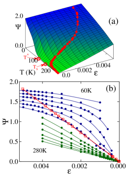
Figure 1: (color online) Monte Carlo spin-nematic order parameter, at $\tilde{g}$=$0.16$ and $\tilde{\lambda}$=$0.12$. (a) $\Psi$ vs. $T$ and $\epsilon$, measured at a fixed lattice distortion $\epsilon$ for each $T$ (restricted MC). Shown are the $T^{*}$ (see text) and $T_{S}$ ($\sim T_{N}$) temperatures. Data are for an 8$\times$8 cluster with TCA+TBC (PBC 8$\times$8 clusters with ED give similar results). Red points are the equilibrium values using unrestricted MC with ED and PBC 8$\times$8 clusters. (b) $\Psi$ vs. $\epsilon$ at fixed temperatures, illustrating their nearly linear relation in unrestricted MC (red), and also the linear slopes of the restricted MC curves (green/blue) close to $T_{S}$. Results are obtained with ED/PBC 8$\times$8 clusters. Note that the number of green/blue points vastly outnumbers the number of red points, highlighting how much more demanding this effort has been than in PRL-2013 .

Figure 1(b) contains the (restricted) MC measured spin-nematic order parameter versus the (fixed) lattice distortion $\epsilon$, at various temperatures. In a wide range of temperatures, a robust linear behavior is observed and $\chi_{s}$ can be easily extracted numerically. Figure 1(b) is similar to the experimental results in Fig. 2A of Ref. fisher-science . The equilibrium result with both spins and lattice optimized (unrestricted MC) is also shown (red squares).

Our main result is presented in Fig. 2, where the numerically calculated $\chi_{s}$ vs. $T$ is displayed, at the realistic couplings used in previous investigations PRL-2013 . In remarkable agreement with experiments, $\chi_{s}$ grows when cooling down and it develops a sharp peak at $T_{S}$ (compare with Fig. 2B of Ref. fisher-science ). These results were obtained via two different procedures (standard ED and the TCA+TBC), and for two lattice sizes, indicating that systematic errors (such as size effects) are small.

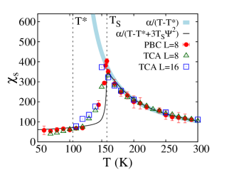
Figure 2: (color online) Nematic susceptibility $\chi_{s}$ of the SF model vs. temperature $T$ (circles, triangles, and squares) obtained from Fig. 1(b), at the realistic couplings $\tilde{g}$=$0.16$ and $\tilde{\lambda}$=$0.12$ ($\alpha$=$\tilde{g}$/$a_{0}$). Two MC techniques were employed: “PBC L=8” is the standard MC method with ED in the fermions at every step, using 8$\times$8 clusters with PBC. “TCA L=8” and “TCA L=16” correspond to the TCA+TBC method on L$\times$L clusters. Size effects are small. Also shown are two GL fits: the light blue (thick) line displays the Curie-Weiss equation $\chi_{s}\approx{\tilde{g}\over{a_{0}(T-T^{*})}}$, indicating a divergence at a lower temperature $T^{*}$, characteristic of the electronic sector alone. At $T\leq T_{S}$, the lattice follows the electronic sector. The black (thin) line is Eq.(2) with the $3T_{S}\Psi^{2}$ correction (see text) T8T16 .

Analysis of $\chi_{s}$ results. Supplementing the computational results, here Ginzburg-Landau (GL) calculations were also performed, similarly as in fisher-science for experiments. Note that the previous GL analysis considered only a generic nematic order parameter while our study separates the spin and orbital contributions. The rather complex numerical results can be rationalized quantitatively by this procedure. The results for $\chi_{s}$ (Fig. 2) are well fitted quantitatively for $T>T_{S}$, and qualitatively for $T<T_{S}$, by the expression:

$$\chi_{s}=\frac{\tilde{g}}{a_{0}[(T-T^{*})+3T_{S}\Psi^{2}]},$$ (2)

where $T_{S}$=$158$ K, $T^{*}$=$105$ K, and $a_{0}$$\sim$$0.093$. $T^{*}$ and $a_{0}$ are here mere fitting parameters, but the GL analysis SM shows that $a_{0}$ arises from the GL quadratic term $a\Psi^{2}/2$ in a second order transition where $a=a_{0}(T-T^{*})$. $\Psi$ is the equilibrium value from unrestricted MC simulations [red, Fig. 1(a)] and it is $T$ dependent. For $T\geq T_{S}$, $\Psi$ vanishes and $\chi_{s}$ exhibits Curie-Weiss behavior, in excellent agreement with the experimental $\chi^{exp}$ fisher-science .

Let us discuss the meaning of the fitting parameter $T^{*}$:

(1) From Fig. 1(b), the unrestricted numerical results at $T=T_{S}$ indicate a linear relation between $\Psi$ and $\epsilon$ (while individually both behave as order parameters, i.e. they change fast near $T_{S}$). $\epsilon=\epsilon(T)$ because the lattice is equilibrated together with the spins. However, this nearly temperature independent ratio $\Psi/\epsilon$=$K$ ($\sim$$360$) depends on couplings: comparing results at several $\tilde{g}$s, it is empirically concluded that $K={\hat{c}\over{\tilde{g}}}$ (constant $\hat{c}$).

Note also that $\chi_{s}$ depends on the partial derivative ${\partial\Psi/{\partial\epsilon}}|_{\epsilon_{0}}$, since $\chi_{s}$ is obtained at a constant $T$ varying $\epsilon$ via strain to match the procedure followed in experiments fisher-science , in the vicinity of the equilibrium point $\epsilon_{0}$ [$\chi_{s}$ arises from the green/blue curves of Fig. 1(b), not from the red equilibrium curve]. While these slopes (restricted vs. unrestricted MC) are in general different, both become very similar at $T\sim T_{S}$ where it can be shown analytically that these derivatives are indeed almost the same SM . Thus, at $T_{S}$: ${d\Psi\over{d\epsilon}}={{\hat{c}}\over{\tilde{g}}}\approx{\partial\Psi\over{\partial\epsilon}}|_{\epsilon_{0}}=\chi_{s}$. This relation can be independently deduced from the GL analysis, Eq.(S18), with $\hat{c}$=$c_{0}$, and $c_{0}$ arising from $c_{0}\epsilon^{2}/2$ in the free energy, providing physical meaning to parameters in the MC fits.

(2) Since the numerical susceptibility $\chi_{s}$ can be fit well by Eq.(2) including at $T_{S}$ where $\Psi=0$, then $T_{S}=T^{*}+{\tilde{g}^{2}\over{a_{0}{\hat{c}}}}$ fisher-science ; kasahara ; SM . Comparing with Eq.(S21), $\hat{c}$ is again identified with the uncoupled shear elastic modulus $c_{0}$. In addition, from PRL-2012 it is known that at $\tilde{g}$=$\tilde{\lambda}$=$0$ there is no nematic regime and $T_{S}$=$T_{N}$, the Néel temperature. Then, $T_{N}=T^{*}+{\tilde{g}^{2}\over{a_{0}c_{0}}}$, that at $\tilde{g}=0$ leads to the important conclusion that the scale $T^{*}$ is simply equal to the Néel temperature of the purely electronic SF model. In previous work PRL-2012 it was reported that $T_{N}$ at $\tilde{g}$=$\tilde{\lambda}$=$0$ is $\sim$100-110 K, in remarkable agreement with the fitting value of $T^{*}$ obtained independently. Thus, in the Curie-Weiss formula $T^{*}$ is solely determined by the magnetic properties of the purely electronic system. This suggests that the magnetic DOF in the SF model plays a leading role to explain the nematic state of Ba(Fe_1-xCo_x)₂As₂ fisher-science . However, the lattice/orbital DOS are also crucial to boost the critical temperature from $T^{*}$$\sim$$105$ K to $T_{S}$$\sim$$158$ K orbitalsusce .

$T_{S}$ vs. $\tilde{\lambda}$. The study in Figs. 1(a,b) was repeated for other $\tilde{\lambda}$s. It was observed that $\hat{c}$ varies with $\tilde{\lambda}$, compatible with the GL analysis where ${\hat{c}}(\tilde{\lambda})=c_{0}(1-{\tilde{\lambda}^{2}\over{e_{0}c_{0}}})$, Eq.(S35). At small $\tilde{\lambda}$, the total (unrestricted MC) and partial (restricted MC) derivatives of $\Psi$ with respect to $\epsilon$ are still approximately equal at $T\approx T_{S}$ SM . Then, $\chi_{s}\approx{c(\tilde{\lambda})/{\tilde{g}}}=\frac{\tilde{g}}{a_{0}(T_{S}-T^{*})}$, leading to the novel result

$$T_{S}=T^{*}+{\tilde{g}^{2}\over{a_{0}c_{0}(1-{\tilde{\lambda}^{2}\over{c_{0}e_{0}}})}}.$$ (3)

Numerically, it was found that $a_{0}$$\sim$$0.093$, $c_{0}$$\sim$$60$ $e_{0}$=$0.015$, and $T^{*}$=$105$ K, for $\tilde{g}$=$0.16$. In practice, it was observed that Eq.(3) fits remarkably well the numerical values for $T_{S}$ in the $\tilde{\lambda}$-range studied showing that the GL approach provides an excellent rationalization of the numerical results. This is shown explicitly in Fig. 3(a).

Spin structure factors and pseudogaps. In Fig. 3(b), the MC-calculated spin structure factor $S({\bf k})$ at both $(\pi,0)$ and $(0,\pi)$ are shown. The results illustrate the development of short-range magnetic order upon cooling with two coexisting wavevectors. Within the error bars, given roughly by the oscillations in the plot, these results indicate that the two wavevectors develop with equal weight upon cooling approximately starting at $T_{PG}$ where the pseudogap develops (see below) note .

Figure 3: (color online) (a) The MC structural transition temperature $T_{S}$ vs. the orbital-lattice coupling $\tilde{\lambda}$, at fixed $\tilde{g}=0.16$. The continuous line is the fit in Eq.(3), from the GL equations. (b) Spin structure factor $S({\bf k})$ vs. $T$ for the two magnetic wavevectors of relevance. Results were obtained via MC simulations on PBC 8$\times$8 clusters. $T_{PG}$ is the pseudogap temperature [Fig. 3(c)]. (c) Density of states $N(\omega)$ (symmetrized) from unrestricted MC simulations on 8$\times$8 clusters ($\tilde{g}$=$0.16$; $\tilde{\lambda}$=$0.12$), at various $T$s. Results at $T_{S}$=$158$ K are in red. $T_{PG}$$\sim$$174$ K (blue) is the crossover $T$ where the pseudogap opens at the Fermi level ($\omega$-$\mu$=$0.0$) upon cooling.

In the spin-fermion model, dynamical observables can be easily calculated. In particular, the density of states $N(\omega)$ is shown in Fig. 3(c). This figure indicates the presence of a Fermi-level pseudogap (PG) in a wide temperature range, as in photoemission and infrared experiments PG-exper . A zero temperature pseudogap is to be expected: Hartree-Fock studies of the multiorbital Hubbard model rong already detected such a feature. However, our finite temperature studies reveal that upon cooling this pseudogap develops at a $T_{PG}$ clearly above $T_{S}$. The pseudogap is present when short-range spin correlations are present [Fig. 3(b)]: the “nematic fluctuations” regime is basically the $T$-range where $(\pi,0)$/$(0,\pi)$ magnetic fluctuations exist. The coupling to the lattice creates concomitant local orthorrombic distortions: the region between $T_{S}$ and $T_{PG}$ is tetragonal only on average egami . All these results are in good agreement with recent scanning tunneling spectroscopy studies of NaFeAs rosenthal .

Conclusions. Our combined numerical and analytical study of the spin fermion model leads to results in agreement with the experimentally measured nematic susceptibility of Ba(Fe_1-xCo_x)₂As₂ fisher-science . In our analysis, which was time consuming and required a new MC setup, magnetism is the main driver, but the lattice/orbital are crucial to boost critical temperatures. For spins coupled to the lattice our spin-nematic susceptibility has a Curie-Weiss behavior for $T>T_{S}$ governed by a $T^{*}$ which we here identify as the critical $T_{N}$ of the purely electronic sector, which is preexisting to the introduction of the lattice. For realistic nonzero electron-lattice couplings, the lattice induces a nematic/structural transition at a higher temperature $T_{S}$. The addition of an orbital-lattice coupling $\tilde{\lambda}$ further increases $T_{S}$, although the Curie-Weiss behavior continues being regulated by $T^{*}$. Our main prediction is that whenever fluctuating nematic order is observed, inelastic neutron scattering for the same sample should also reveal the existence of short-range magnetic order: nematic fluctuations, pseudogap, and short-range antiferromagnetic order should all develop simultaneously in these materials.

Acknowledgments. Conversations with Weicheng Lv are acknowledged. S.L., A.M., and N.P. were supported by the National Science Foundation Grant No. DMR-1104386. E.D. and A.M. were supported by the U.S. Department of Energy, Office of Basic Energy Sciences, Materials Sciences and Engineering Division.

S1 Supplementary Material

This Supplementary Material provides additional detail about results presented in the main text. In particular, it includes: the full Hamiltonian, the derivations of equations deduced in the Ginzburg-Landau context, and Monte Carlo results at the (unphysically large PRL-2013-SM ) coupling $\tilde{\lambda}=0.84$.

S1 Full Hamiltonian

The full Hamiltonian of the spin-fermion model with lattice interactions incorporated is here provided. The same Hamiltonian was also used in Ref. PRL-2013-SM . The model is given by:

$$H_{\rm SF}=H_{\rm Hopp}+H_{\rm Hund}+H_{\rm Heis}+H_{\rm SL}+H_{\rm OL}+H_{\rm Stiff}.$$ (S1)

The hopping component is made of three contributions,

$$H_{\rm Hopp}=H_{xz,yz}+H_{xy}+H_{xz,yz;xy}.$$ (S2)

The first term involves the $xz$ and $yz$ orbitals:

$$\begin{split}H_{xz,yz}&=\{-t_{1}\sum_{{\bf i},\sigma}(d^{\dagger}_{{\bf i},xz,\sigma}d^{\phantom{\dagger}}_{{\bf i}+\hat{y},xz,\sigma}+d^{\dagger}_{{\bf i},yz,\sigma}d^{\phantom{\dagger}}_{{\bf i}+\hat{x},yz,\sigma})\\ &-t_{2}\sum_{{\bf i},\sigma}(d^{\dagger}_{{\bf i},xz,\sigma}d^{\phantom{\dagger}}_{{\bf i}+\hat{x},xz,\sigma}+d^{\dagger}_{{\bf i},yz,\sigma}d^{\phantom{\dagger}}_{{\bf i}+\hat{y},yz,\sigma})\\ &-t_{3}\sum_{{\bf i},\hat{\mu}\not=\hat{\nu},\sigma}(d^{\dagger}_{{\bf i},xz,\sigma}d^{\phantom{\dagger}}_{{\bf i}+\hat{\mu}+\hat{\nu},xz,\sigma}+d^{\dagger}_{{\bf i},yz,\sigma}d^{\phantom{\dagger}}_{{\bf i}+\hat{\mu}+\hat{\nu},yz,\sigma})\\ &+t_{4}\sum_{{\bf i},\sigma}(d^{\dagger}_{{\bf i},xz,\sigma}d^{\phantom{\dagger}}_{{\bf i}+\hat{x}+\hat{y},yz,\sigma}+d^{\dagger}_{{\bf i},yz,\sigma}d^{\phantom{\dagger}}_{{\bf i}+\hat{x}+\hat{y},xz,\sigma})\\ &-t_{4}\sum_{{\bf i},\sigma}(d^{\dagger}_{{\bf i},xz,\sigma}d^{\phantom{\dagger}}_{{\bf i}+\hat{x}-\hat{y},yz,\sigma}+d^{\dagger}_{{\bf i},yz,\sigma}d^{\phantom{\dagger}}_{{\bf i}+\hat{x}-\hat{y},xz,\sigma})\\ &+h.c.\}-\mu\sum_{\bf i}(n_{{\bf i},xz}+n_{{\bf i},yz}).\end{split}$$ (S3)

The second term contains the hoppings related with the $xy$ orbital:

$$\begin{split}H_{xy}=&\ t_{5}\sum_{{\bf i},{\hat{\mu}},\sigma}(d^{\dagger}_{{\bf i},xy,\sigma}d^{\phantom{\dagger}}_{{\bf i}+\hat{\mu},xy,\sigma}+h.c.)\\ &-t_{6}\sum_{{\bf i},\hat{\mu}\not=\hat{\nu},\sigma}(d^{\dagger}_{{\bf i},xy,\sigma}d^{\phantom{\dagger}}_{{\bf i}+\hat{\mu}+\hat{\nu},xy,\sigma}+h.c.)\\ &+\Delta_{xy}\sum_{\bf i}n_{{\bf i},xy}-\mu\sum_{\bf i}n_{{\bf i},xy},\;\end{split}$$ (S4)

The last hopping term is:

$$\begin{split}H_{\rm xz,yz;xy}=&-t_{7}\sum_{{\bf i},\sigma}[(-1)^{|{\bf i}|}d^{\dagger}_{{\bf i},xz,\sigma}d^{\phantom{\dagger}}_{{\bf i}+\hat{x},xy,\sigma}+h.c.]\\ &-t_{7}\sum_{{\bf i},\sigma}[(-1)^{|{\bf i}|}d^{\dagger}_{{\bf i},xy,\sigma}d^{\phantom{\dagger}}_{{\bf i}+\hat{x},xz,\sigma}+h.c.]\\ &-t_{7}\sum_{{\bf i},\sigma}[(-1)^{|{\bf i}|}d^{\dagger}_{{\bf i},yz,\sigma}d^{\phantom{\dagger}}_{{\bf i}+\hat{y},xy,\sigma}+h.c.]\\ &-t_{7}\sum_{{\bf i},\sigma}[(-1)^{|{\bf i}|}d^{\dagger}_{{\bf i},xy,\sigma}d^{\phantom{\dagger}}_{{\bf i}+\hat{y},yz,\sigma}+h.c.]\\ &-t_{8}\sum_{{\bf i},\sigma}[(-1)^{|{\bf i}|}d^{\dagger}_{{\bf i},xz,\sigma}d^{\phantom{\dagger}}_{{\bf i}+\hat{x}+\hat{y},xy,\sigma}+h.c.]\\ &+t_{8}\sum_{{\bf i},\sigma}[(-1)^{|{\bf i}|}d^{\dagger}_{{\bf i},xy,\sigma}d^{\phantom{\dagger}}_{{\bf i}+\hat{x}+\hat{y},xz,\sigma}+h.c.]\\ &-t_{8}\sum_{{\bf i},\sigma}[(-1)^{|{\bf i}|}d^{\dagger}_{{\bf i},xz,\sigma}d^{\phantom{\dagger}}_{{\bf i}+\hat{x}-\hat{y},xy,\sigma}+h.c.]\\ &+t_{8}\sum_{{\bf i},\sigma}[(-1)^{|{\bf i}|}d^{\dagger}_{{\bf i},xy,\sigma}d^{\phantom{\dagger}}_{{\bf i}+\hat{x}-\hat{y},xz,y\sigma}+h.c.]\\ &-t_{8}\sum_{{\bf i},\sigma}[(-1)^{|{\bf i}|}d^{\dagger}_{{\bf i},yz,\sigma}d^{\phantom{\dagger}}_{{\bf i}+\hat{x}+\hat{y},xy,\sigma}+h.c.]\\ &+t_{8}\sum_{{\bf i},\sigma}[(-1)^{|{\bf i}|}d^{\dagger}_{{\bf i},xy,\sigma}d^{\phantom{\dagger}}_{{\bf i}+\hat{x}+\hat{y},yz,\sigma}+h.c.]\\ &+t_{8}\sum_{{\bf i},\sigma}[(-1)^{|{\bf i}|}d^{\dagger}_{{\bf i},yz,\sigma}d^{\phantom{\dagger}}_{{\bf i}+\hat{x}-\hat{y},xy,\sigma}+h.c.]\\ &-t_{8}\sum_{{\bf i},\sigma}[(-1)^{|{\bf i}|}d^{\dagger}_{{\bf i},xy,\sigma}d^{\phantom{\dagger}}_{{\bf i}+\hat{x}-\hat{y},yz,\sigma}+h.c.].\end{split}$$ (S5)

In the equations above, the operator $d^{\dagger}_{{\bf i},\alpha,\sigma}$ creates an electron at site ${\bf i}$ of the two-dimensional lattice of irons. The orbital index is $\alpha=$ $xz$, $yz$, or $xy$, and the $z$-axis spin projection is $\sigma$. The chemical potential used to regulate the electronic density is $\mu$. The symbols ${\hat{x}}$ and ${\hat{y}}$ denote vectors along the axes that join NN atoms. The values of the hoppings $t_{i}$ are from Ref. three-SM and they are reproduced in Table 1, including also the value of the energy splitting $\Delta_{xy}$.

Table 1: Values of the parameters that appear in the tight-binding portion of the three-orbital model Eqs.(S3) to (S5). The overall energy unit is electron volts.

$t_{1}$	$t_{2}$	$t_{3}$	$t_{4}$	$t_{5}$	$t_{6}$	$t_{7}$	$t_{8}$	$\Delta_{xy}$
0.02	0.06	0.03	$-0.01$	$0.2$	0.3	$-0.2$	$0.1$	0.4

The remaining terms of the Hamiltonian have been briefly discussed in the main text. The symbols $\langle\rangle$ denote NN while $\langle\langle\rangle\rangle$ denote NNN. The rest of the notation is standard.

$$H_{\rm Hund}=-{J_{\rm H}}\sum_{{\bf i},\alpha}{{{\bf S}_{\bf i}}\cdot{{\bf s}_{{\bf i},\alpha}}},$$ (S6)

$$H_{\rm Heis}=J_{{\rm NN}}\sum_{\langle{\bf ij}\rangle}{\bf S}_{{\bf i}}\cdot{\bf S}_{{\bf j}}+J_{{\rm NNN}}\sum_{\langle\langle{\bf im}\rangle\rangle}{\bf S}_{{\bf i}}\cdot{\bf S}_{{\bf m}},$$ (S7)

$$H_{\rm SL}=-g\sum_{\bf i}\Psi_{\bf i}\epsilon_{\bf i},$$ (S8)

$$H_{\rm OL}=-\lambda\sum_{\bf i}\Phi_{\bf i}\epsilon_{\bf i},$$ (S9)

$$\begin{split}H_{\rm Stiff}={1\over{2}}k\sum_{\bf i}\sum_{\nu=1}^{4}(|{\bf R}^{\bf i\nu}_{Fe-As}|-R_{0})^{2}+\\ +k^{\prime}\sum_{<{\bf ij}>}[({a_{0}\over{R^{\bf ij}_{Fe-Fe}}})^{12}-2({a_{0}\over{R^{\bf ij}_{Fe-Fe}}})^{6}].\end{split}$$ (S10)

The $\mathcal{O}_{rth}$ strain $\epsilon_{\bf i}$ is defined as:

$$\epsilon_{\bf i}={1\over{4\sqrt{2}}}\sum_{\nu=1}^{4}(|\delta_{\bf i,\nu}^{y}|-|\delta_{\bf i,\nu}^{x}|),\vspace{-0.1cm}$$ (S11)

where $\delta_{\bf i,\nu}^{x}$($\delta_{\bf i,\nu}^{y}$) is the component along $x$ ($y$) of the distance between the Fe atom at site ${\bf i}$ of the lattice and one of its four neighboring As atoms that are labeled by the index $\nu=1,2,3,4$. For more details of the notation used see Ref. PRL-2013-SM , where the technical aspects on how to simulate an orthorrombic distortion can also be found.

S2 Ginzburg-Landau phenomenological approach

In this section, the Monte Carlo data gathered for the spin-fermion model will be described via a phenomenological Ginzburg-Landau (GL) approach, to provide a more qualitative description of those numerical results. More specifically, the free energy $F$ of the SF model will be (approximately) written in terms of the spin-nematic order parameter $\Psi$, the orbital-nematic order parameter $\Phi$, and the orthorhombic strain $\epsilon$, as in GL descriptions. In previous literature a single nematic order parameter was considered without separating its magnetic and orbital character fisher-science-SM ; kasahara-SM ; fernandes2-SM . In addition, it was necessary to formulate assumptions about the order of the nematic and structural transitions. In our case, the MC results in this and previous publications are used as guidance to address this matter at the free energy level. More specifically, a second order magnetic transition was previously reported for the purely electronic system PRL-2012-SM . Thus, the spin-nematic portion of $F$ should display a free energy with a second order phase transition.

With regards to the terms involving $\epsilon$, the MC results of Ref. PRL-2013-SM showed that the coupling of the spin-nematic order parameter to the lattice leads to a weak first order (or very sharp second order) nematic and structural transition. Naively, this implies that the order $\epsilon^{4}$ term should have a negative coefficient. However, since in our numerical simulations a Lennard-Jones potential is used for the elastic term, then the sign of the quartic term is fixed and it happens to be positive. However, considering that the $\epsilon$ displacements are very small and the transition is weakly first order at best, then just the harmonic (second order) approximation should be sufficient for $\epsilon$.

After all these considerations, the free energy is given by:

$$F={a\over{2}}\Psi^{2}+{b\over{4}}\Psi^{4}+{c\over{2}}\epsilon^{2}+{e\over{2}}\Phi^{2}+{f\over{4}}\Phi^{4}$$ (S12)

$$-\tilde{g}\Psi\epsilon-\tilde{\lambda}\Phi\epsilon-h\epsilon,$$ (S13)

where $a$, $b$, $c$, $e$, and $f$ are the coefficients of the many terms of the three order parameters, while $\tilde{g}$ and $\tilde{\lambda}$ are the coupling constants of the lattice with the spin and orbital degrees of freedom as described in the main text. Since this and previous MC studies PRL-2012-SM ; PRL-2013-SM showed that there is no long-range orbital order in the ground state of the SF model, at least in the range of couplings investigated, then a positive quartic term is used for this order parameter. The parameter $h$ denotes an external stress, as explained in Ref. fisher-science-SM . Note that in principle another term, and associated coupling constant, ${\tilde{\alpha}}\Psi\Phi$ should be included in $F$. This term will affect the orbital susceptibility deduced at the end of this subsection. However, adding this term requires varying another parameter in the SF model MC simulation, thus increasing substantially the time demands for this project. As a consequence, this addition is postponed for the near future.

As explained in the main text, our MC results indicate that the leading order parameter guiding the results is the spin-nematic $\Psi$. Thus, it is reasonable to assume that only the coefficient $a$ depends on temperature as $a=a_{0}(T-T^{*})$, while other parameters, such as $c=c_{0}$ (the uncoupled shear elastic modulus) and $e=e_{0}$, are approximately $T$-independent.

For the special case $\tilde{g}=\tilde{\lambda}=0$ the critical temperature $T^{*}$ for the magnetic transition can be obtained by setting to zero the derivative of $F$ with respect to $\Psi$:

$${\partial F\over{\partial\Psi}}=a\Psi+b\Psi^{3}=0.$$ (S14)

Then, for $T\leq T^{*}$ the order parameter is given by

$$\Psi=\sqrt{{a_{0}\over{b}}(T^{*}-T)}.$$ (S15)

The equation above is valid only when $\Psi$ is small, i.e. close to the transition temperature from below. Additional terms in the free energy would be needed as $T\rightarrow 0$ since in that limit $|\Psi|=2$.

Now consider the case when $\tilde{g}$ is nonzero, still keeping $\tilde{\lambda}=0$. Setting to zero the derivative of $F$ with respect to $\Psi$ and $\epsilon$ leads to (for $h=0$):

$${\partial F\over{\partial\epsilon}}=c_{0}\epsilon-\tilde{g}\Psi=0,$$ (S16)

$${\partial F\over{\partial\Psi}}=a\Psi+b\Psi^{3}-\tilde{g}\epsilon=0.$$ (S17)

From Eq.(S16),

$$\Psi={c_{0}\over{\tilde{g}}}\epsilon,$$ (S18)

which reproduces the linear relation obtained numerically before, see Fig. 1(b) main text, with a slope now explicitly given in terms of $\tilde{g}$ and a constant that now can be identified with the bare shear elastic modulus $c_{0}$.

Solving for $\epsilon$ in Eq.(S17) and introducing the result in Eq.(S16) leads to:

$$(a-{\tilde{g}^{2}\over{c_{0}}})\Psi+b\Psi^{3}=0,$$ (S19)

where it is clear that $a$ becomes renormalized due to the coupling to the lattice. The transition now occurs at a renormalized temperature $T_{S}$ that satisfies:

$$a_{0}(T-T_{S})=a-{\tilde{g}^{2}\over{c_{0}}}=a_{0}(T-T^{*})-{\tilde{g}^{2}\over{c_{0}}}.$$ (S20)

From the expression above, it can be shown that the new nematic transition occurs at

$$T_{S}=T^{*}+{\tilde{g}^{2}\over{a_{0}c_{0}}},$$ (S21)

and clearly $T_{S}>T^{*}$. Note that Eq.(S21) has been obtained in previous GL analysis, but in those studies a generic nematic coupling appeared in the numerator of the second term while here, more specifically, we identify $\tilde{g}$ with the spin-nematic coupling to the lattice.

Reciprocally, solving for $\Psi$ in Eq.(S16) and introducing the result in Eq.(S17) leads to:

$${a\over{\tilde{g}}}[(c_{0}-{\tilde{g}^{2}\over{a}})\epsilon+{bc_{0}^{3}\over{\tilde{g}^{2}a}}\epsilon^{3}]=0,$$ (S22)

where, due to the coupling to the lattice, now the shear constant is renormalized and an effective quartic term is generated for the lattice free energy. The effective shear elastic modulus $c_{66}$ becomes temperature dependent and it is given by:

$$c_{66}=c_{0}-{\tilde{g}^{2}\over{a_{0}(T-T^{*})}},$$ (S23)

that vanishes at $T=T_{S}$. Thus, the structural transition occurs at the same critical temperature $T_{S}$ of the nematic transition.

To obtain the spin-nematic susceptibility, the second derivative of $F$ with respect to $\Psi$ and $h$ is set to zero:

$${\partial^{2}F\over{\partial h\partial\Psi}}=a{\partial\Psi\over{\partial h}}+3b\Psi^{2}{\partial\Psi\over{\partial h}}-\tilde{g}{\partial\epsilon\over{\partial h}}=0,$$ (S24)

and then

$$\chi_{s}={\partial\Psi\over{\partial\epsilon}}={{\partial\Psi\over{\partial h}}\over{{\partial\epsilon\over{\partial h}}}}={\tilde{g}\over{a+3b\Psi^{2}}}={\tilde{g}\over{a_{0}(T-T^{*})+3b\Psi^{2}}}.$$ (S25)

This is an important equation that was used in the main text to rationalize the MC numerical results. In the range $T\geq T_{S}$, i.e. when $\Psi=0$, the spin-nematic susceptibility clearly follows a Curie-Weiss behavior. In practice, it has been observed that $b=a_{0}T_{S}$ to a good approximation.

Consider now the case when the orbital-lattice coupling $\tilde{\lambda}$ is nonzero as well. Now

$${\partial F\over{\partial\epsilon}}=c_{0}\epsilon-\tilde{g}\Psi-\tilde{\lambda}\Phi=0,$$ (S26)

$${\partial F\over{\partial\Psi}}=a\Psi+b\Psi^{3}-\tilde{g}\epsilon=0,$$ (S27)

and a new equation is available:

$${\partial F\over{\partial\Phi}}=e_{0}\Phi+f\Phi^{3}-\tilde{\lambda}\epsilon=0.$$ (S28)

Solving for $\Psi$ in Eq.(S26) leads to:

$$\Psi={c_{0}\epsilon-\tilde{\lambda}\Phi\over{\tilde{g}}},$$ (S29)

while solving for $\epsilon$ in Eq.(S27) leads to:

$$\epsilon={a\Psi+b\Psi^{3}\over{\tilde{g}}}.$$ (S30)

Introducing Eq.(S30) into Eq.(S29), $\Phi$ is obtained in terms of $\Psi$ as follows:

$$\Phi=({c_{0}\over{\tilde{\lambda}\tilde{g}}})[(a-{\tilde{g}^{2}\over{c_{0}}})\Psi+b\Psi^{3}].$$ (S31)

Introducing Eqs.(S30) and (S31) into Eq.(S28) a renormalized equation for $\Psi$ is obtained:

$$[{e_{0}c_{0}\over{\tilde{\lambda}\tilde{g}}}(a-{\tilde{g}^{2}\over{c_{0}}})-{\tilde{\lambda}a\over{\tilde{g}}}]\Psi\ +[{e_{0}c_{0}\over{\tilde{\lambda}\tilde{g}}}b-{\tilde{\lambda}b\over{\tilde{g}}}+{fc_{0}^{3}\over{\tilde{\lambda}^{3}\tilde{g}^{3}}}(a-{\tilde{g}^{2}\over{c_{0}}})^{3}\ ]\Psi^{3}=0.$$ (S32)

Then, at $T=T_{S}$ the effective coefficient of the linear term in $\Psi$ provides the new transition temperature:

$$a_{0}(T-T_{S})=a-{e_{0}\tilde{g}^{2}\over{e_{0}c_{0}-\tilde{\lambda}^{2}}}.$$ (S33)

Using that $a=a_{0}(T-T^{*})$, the dependence of the critical temperature with the two coupling constants $\tilde{g}$ and $\tilde{\lambda}$ can be obtained:

$$T_{S}=T^{*}+{\tilde{g}^{2}\over{a_{0}c_{0}(1-{\tilde{\lambda}^{2}\over{c_{0}e_{0}}})}}.$$ (S34)

This is another interesting formula that nicely describes the MC results, as shown in the main text. Equation(S34) is a novel result that shows that $T_{S}$ depends in a different way on the spin-lattice ($\tilde{g}$) and the orbital-lattice ($\tilde{\lambda}$) couplings. Moreover, an effective $\tilde{\lambda}$-dependent elastic modulus $c(\tilde{\lambda})$ can be defined as

$$c(\tilde{\lambda})=c_{0}-{\tilde{\lambda}^{2}\over{e_{0}}}.$$ (S35)

In addition, the effective shear elastic modulus is now given by

$$c_{66}=c_{0}-{\tilde{\lambda}^{2}\over{e_{0}}}-{\tilde{g}^{2}\over{a_{0}(T-T^{*})}},$$ (S36)

which vanishes at the $T_{S}$ given by Eq.(S34).

The spin-nematic susceptibility is still given by Eq.(S25) with the dependence on $\tilde{\lambda}$ embedded in the actual values of $\Psi$. The orbital-nematic susceptibility is obtained from Eq.(S28) as

$${\partial^{2}F\over{\partial h\partial\Phi}}=(e_{0}+3f\Phi^{2}){\partial\Phi\over{\partial h}}-\tilde{\lambda}\ {\partial\epsilon\over{\partial h}}-\tilde{\alpha}{\partial\Phi\over{\partial h}}=0.$$ (S37)

In the absence of an explicit coupling $\tilde{\alpha}$ between the spin-nematic and orbital order parameters, then the orbital-nematic susceptibility becomes:

$$\chi_{o}={\partial\Phi\over{\partial\epsilon}}={{\partial\Phi\over{\partial h}}\over{{\partial\epsilon\over{\partial h}}}}={\tilde{\lambda}\over{e_{0}+3f\Phi^{2}}}.$$ (S38)

S3 Partial and total derivatives at $T_{S}$

The partial derivative in the definition of $\chi_{s}$ is at constant $T$ varying $\epsilon$ and it is evaluated at equilibrium $\epsilon=\epsilon_{0}$. The slopes of the green and blue curves of Fig. 1(b) in the main text provide this derivative. On the other hand, the results of Fig. 1(b) in equilibrium (slope of the red points curve) provide the full derivative ${d\Psi\over{d\epsilon}}$. Since $\epsilon$=$\epsilon(T)$, their relation is

$${d\Psi\over{d\epsilon}}={\partial\Psi\over{\partial\epsilon}}|_{\epsilon_{0}}+{\partial\Psi\over{\partial T}}|_{\epsilon_{0}}{\partial T\over{\partial\epsilon}}|_{\epsilon_{0}}=\chi_{s}+{{\partial\Psi\over{\partial T}}|_{\epsilon_{0}}\over{{\partial\epsilon\over{\partial T}}|_{\epsilon_{0}}}},$$ (S39)

where ${\partial\Psi\over{\partial T}}$ is performed at constant $\epsilon$ and ${\partial\epsilon\over{\partial T}}|_{\epsilon_{0}}$ is performed at constant $\Psi$. In general, the partial and total derivatives of $\Psi$ with respect to $\epsilon$ can differ from one another. However, at small $\tilde{\lambda}$ the structural transition is weakly first order PRL-2013-SM (or a very sharp second order) and then when $T\approx T_{S}$ the lattice distortion $\epsilon$ rapidly jumps from 0 to a finite value. This means that ${\partial\epsilon\over{\partial T}}|_{\epsilon_{0}}$ is very large while ${\partial\Psi\over{\partial T}}|_{\epsilon_{0}}$ remains finite since it is performed at fix $\epsilon$. Thus, at $T\approx T_{S}$, the partial and total derivatives are almost the same. This can be seen in Fig. 1(b) of the main text where the slopes of the green curves at $\epsilon=0$, when they cross the equilibrium line, are smaller than the equilibrium slope $K$ but increase with decreasing $T$ until it becomes equal to $K$ at $T=T_{S}$ (red line). The slopes of the blue curves at the finite value of $\epsilon$ where they cross the equilibrium line are smaller than $K$ and decrease with decreasing $T$.

S4 Spin-nematic susceptibility at large $\tilde{\lambda}$

To investigate in more detail the potential role of orbital order in the spin-nematic susceptibility, simulations were repeated for a robust $\tilde{\lambda}=0.84$, keeping the other electron-lattice coupling fixed as $\tilde{g}=0.16$. Results are shown in Fig. S1. The increase of $\tilde{\lambda}$ substantially increases $T_{S}$, which is to be expected since now the electron-lattice coupling is larger PRL-2013-SM . However, above $T_{S}$ still the results can be well fit by a Curie-Weiss law, with a divergence at $T^{*}$ which is the critical temperature of the purely electronic system, as described in the main text. Even the coefficient $a_{0}$ in the fit is almost identical to that of the case $\tilde{\lambda}=0.12$, in Fig. 2. The second fit, with the 3$T_{S}$$\Psi^{2}$ correction, is still reasonable. In summary, as long as $\tilde{\lambda}$ is not increased to such large values that the low-temperature ground state is drastically altered, the computational results can still be analyzed via the GL formalism outlined here and in the main text, with a $T^{*}$ that originates in the $(\pi,0)$ magnetic transition of the purely electronic sector.

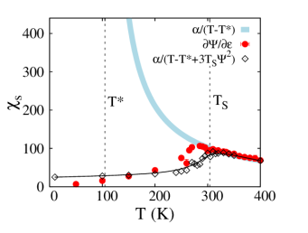
Figure S1: (color online) Spin-nematic susceptibility $\chi_{s}$ vs. temperature $T$ (red circles) obtained from Fig. S2(b) (at $\tilde{g}$=$0.16$ and $\tilde{\lambda}$=$0.84$). The standard MC technique on an 8$\times$8 cluster with PBC was employed (involving ED of the fermions at every MC step). Also shown are two GL fits, as also employed in Fig. 2. The blue (thick) line indicates a divergence at a temperature $T^{*}$ (lower than $T_{S}$) characteristic of the electronic sector alone. In the range $T\leq T_{S}$, the lattice follows the electronic behavior. The black (thin) line and black tilted square points are a fit including the $3T_{S}\Psi^{2}$ correction (see text in the previous section of this Suppl. Material). The fitting parameters are $T^{*}=105$ K and $T_{S}=304$ K. The actual Néel temperature for $\tilde{g}$=$0.16$ and $\tilde{\lambda}$=$0.84$ is not shown.

For completeness, the plots analog to those of Fig. 1 but in the present case of $\tilde{\lambda}=0.84$ are provided in Fig. S2.

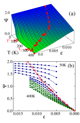
Figure S2: (color online) Spin-nematic order parameter from the MC simulations, at $\tilde{g}$=$0.16$ and $\tilde{\lambda}$=$0.84$. (a) $\Psi$ vs. $T$ and $\epsilon$, measured at a fixed lattice distortion $\epsilon$ for each $T$ (restricted MC). Shown are the $T^{*}$ temperature (see text) and $T_{S}$. Results shown are for an 8$\times$8 cluster with TCA+TBC, but PBC 8$\times$8 clusters with ED give similar results. Red points are the equilibrium values using unrestricted MC with ED and PBC 8$\times$8 clusters. (b) MC results illustrating the relation between $\Psi$ and $\epsilon$ in unrestricted MC (red) and the restricted MC curves (green/blue), parametric with $T$. Results are obtained with ED/PBC 8$\times$8 clusters. Note that $\Psi$ vs. $\epsilon$ (red squares) is no longer linear which is expected because Eq.(S18) is valid only for $~{}\tilde{\lambda}=0$ (and approximately valid for small $\tilde{\lambda}$).

References

- (1) D. C. Johnston, Adv. Phys. 59, 803 (2010).
- (2) P. Dai, J.-P. Hu , and E. Dagotto, Nat. Phys. 8, 709 (2012).
- (3) J-H. Chu, J. G. Analytis, K. De Greve, P. L. McMahon, Z. Islam, Y. Yamamoto, and I. R. Fisher, Science 329, 824 (2010); See also I. R. Fisher, L. Degiorgi, and Z. X. Shen, Rep. Prog. Phys. 74, 124506 (2011).
- (4) E. Fradkin et al., Annu. Rev. Cond. Mat. Phys. 1, 153 (2010).
- (5) R. M. Fernandes et al., Phys. Rev. Lett. 105, 157003 (2010).
- (6) C. Fang, H. Yao, W.-F. Tsai, J.P. Hu, and S. A. Kivelson, Phys. Rev. B 77, 224509 (2008).
- (7) C. Xu, M. Müller, and S. Sachdev, Phys. Rev. B 78, 020501(R) (2008).
- (8) R. M. Fernandes et al., Phys. Rev. B 85, 024534 (2012).
- (9) R. M. Fernandes, A. V. Chubukov, and J. Schmalian, Nature Phys. 10, 97 (2014).
- (10) C.-C. Lee, W.-G. Yin, and Wei Ku, Phys. Rev. Lett. 103, 267001 (2009).
- (11) C.-C. Chen et al., Phys. Rev. B 80, 180418(R) (2009); C.-C. Chen et al., Phys. Rev. B 82, 100504(R) (2010).
- (12) W. Lv, J.S. Wu, and P. Phillips, Phys. Rev. B 80, 224506 (2009); W.-C. Lee et al., Phys. Rev. B 86, 094516 (2012).
- (13) H. Kontani et al., Solid State Comm. 152, 718 (2012); H. Kontani, T. Saito, and S. Onari, Phys. Rev. B 84, 024528 (2011).
- (14) S. Liang, A. Moreo, and E. Dagotto, Phys. Rev. Lett. 111, 047004 (2013).
- (15) W.-G. Yin, C.-C. Lee, and W. Ku, Phys. Rev. Lett. 105, 107004 (2010).
- (16) W. Lv, F. Krüger, and P. Phillips, Phys. Rev. B 82, 045125 (2010).
- (17) S. Liang, G. Alvarez, C. Sen, A. Moreo, and E. Dagotto, Phys. Rev. Lett. 109, 047001 (2012).
- (18) E. Dagotto, T. Hotta, and A. Moreo, Phys. Rep. 344, 1 (2001).
- (19) H. Gretarsson et al., Phys. Rev. B 84, 100509(R) (2011).
- (20) F. Bondino et al., Phys. Rev. Lett. 101, 267001 (2008).
- (21) =- can be regulated by the electron-orbital coupling leading to a in our model larger than the small values reported for spin systems [see Y. Kamiya, N. Kawashima, and C. D. Batista, Phys. Rev. B 84, 214429 (2011); A. L. Wysocki, K. D. Belashchenko, and V. P. Antropov, Nat. Phys. 7, 485 (2011)].
- (22) J-H. Chu, H-H. Kuo, J. G. Analytis, and I. R. Fisher, Science 337, 710 (2012); H. H. Kuo et al., Phys. Rev. B 88, 085113 (2013); and references therein.
- (23) See Supplemental Material at http://link.aps.org/supplemental/xx.xxxx for details of the GL calculations and results at =.
- (24) M. Daghofer et al., Phys. Rev. B 81, 014511 (2010).
- (25) The original definitions of and in PRL-2013 have been multiplied by so that and are both positive here, as assumed in the GL analysis.
- (26) The spin in will only be the localized spin for computational simplicity.
- (27) S. Kumar and P. Majumdar, Eur. Phys. J. B 50, 571 (2006).
- (28) In unrestricted MC employing the ED method on 88 clusters, typically 8,000 thermalization (Th) and up to 100,000 measurement (Ms) steps were used. In restricted MC with ED and 88 clusters, the numbers are 8,000 and 20,000 for Th and Ms steps. In restricted MC using TCA+TBC, 4,000 Th and 4,000 Ms steps were employed for a 1616 cluster with a 44 cluster for the MC updates, while for an 88 (same MC update cluster) the numbers were 20,000 for Th and 20,000 for Ms steps.
- (29) J. Salafranca, G. Alvarez, and E. Dagotto, Phys. Rev. B 80, 155133 (2009).
- (30) The value of is not the same (but close) for 88 and 1616 lattices due to size effects. Then, the fits for each lattice size are carried out with the of each cluster.
- (31) S. Kasahara et al., Nature 486, 382 (2012).
- (32) The orbital-based nematic susceptibility, , was also numerically calculated varying the temperature (not shown). For small , such as , the result is approximately temperature independent and well fit by Eq.(S27) in SM , with and . In other words, the analog of Fig. 1(b) but for the orbital-nematic order parameter presents blue/green/red curves all with very similar slopes. Then, in there is no Curie-Weiss behavior for and in our model the orbital DOF plays a secondary role. This is also in agreement with angle-resolved photoemission experiments that reported a different population of the and orbitals [see T. Shimojima et al., Phys. Rev. Lett. 104, 057002 (2010)], since this Fermi-surface unbalance originates in the rotational symmetry breaking property of the magnetic order as explained in M. Daghofer et al., Phys. Rev. B 81, 180514(R) (2010).
- (33) Note that in the presence of external strain to detwin crystals, some remaining artificial anisotropy may incorrectly suggest that are not degenerate above in neutron scattering, leading to the incorrect conclusion that is (for related observations see C. Dhital et al., Phys. Rev. Lett. 108, 087001 (2012); E. C. Blomberg et al., Phys. Rev. B 85, 144509 (2012)).
- (34) Our results should be compared against the photoemission experiments reported by T. Shimojima et al., Phys. Rev. B 89, 045101 (2014) (see for instance their Figure 6). Infrared studies correlating the presence of a pseudogap with antiferromagnetic fluctuations can also be found in S. J. Moon et al., Phys. Rev. Lett. 109, 027006 (2012).
- (35) Rong Yu et al., Phys. Rev. B 79, 104510 (2009).
- (36) J. L. Niedziela, M. A. McGuire, and T. Egami, Phys. Rev. B 86, 174113 (2012), and references therein.
- (37) E. P. Rosenthal et al., Nature Phys. 10, 225 (2014).

References

- (1) S. Liang, A. Moreo, and E. Dagotto, Phys. Rev. Lett. 111, 047004 (2013).
- (2) M. Daghofer et al., Phys. Rev. B 81, 014511 (2010).
- (3) J-H. Chu, H-H. Kuo, J. G. Analytis, and I. R. Fisher, Science 337, 710 (20121); H. H. Kuo et al., Phys. Rev. B 88, 085113 (2013); and references therein.
- (4) S. Kasahara et al., Nature 486, 382 (2012).
- (5) R. M. Fernandes and J. Schmalian, Supercond. Sci. Technol. 25, 084005 (2012).
- (6) S. Liang, G. Alvarez, C. Sen, A. Moreo, and E. Dagotto, Phys. Rev. Lett. 109, 047001 (2012).