Neumann domination for the Yang-Mills heat equation

Abstract.

Long time existence and uniqueness of solutions to the Yang-Mills heat equation have been proven over a compact 3-manifold with boundary for initial data of finite energy. In the present paper we improve on previous estimates by using a Neumann domination technique that allows us to get much better pointwise bounds on the magnetic field. As in the earlier work, we focus on Dirichlet, Neumann and Marini boundary conditions. In addition, we show that the Wilson Loop functions, gauge invariantly regularized, converge as the parabolic time goes to infinity.

1. Introduction

A gauge invariant regularization method for Wilson loop variables appears to be an unavoidable necessity for construction of quantized Yang-Mills fields. The standard methods of regularizing a quantum field, that have been successful in studying scalar field theories, are inapplicable to gauge fields. Thus a simple weighted average $\int_{\mathbb{R}^{3}}f(x-y)A(y)d^{3}y$ destroys gauge invariance of the gauge potential $A$. Similar expressions, such as $\int_{R^{n}}f(x-y)F(y)d^{n}y$, with $F(y)$ the curvature of $A$, also destroy gauge invariance, both for a space average, with $n=3$, or a Euclidean space-time average, with $n=4$. For a closed curve $C$ in $R^{3}$ the Wilson loop variable, $W_{C}(A)\equiv trace\,T(\exp(\int_{C}A(x)\cdot dx))$, where $T$ denotes time ordering around the loop, is gauge invariant but highly singular as a function of $A$ when $A$ varies over the very large space of typical gauge fields required in the quantized theory. The lattice regularization of these functions of the gauge fields has been the only useful gauge invariant regularization procedure so far but has not produced a continuum limit.

Polyakov [Pol1, Pol2] already observed that the vacuum expectation of continuum Wilson loop variables are likely to be zero for a non-commutative gauge group. They are zero in the electromagnetic case. Nevertheless it has been hoped that the informal symbol, defined as $W_{C}(A)/\langle W_{C}\rangle_{VEV}$, which nominally is identically infinite in absolute value, could play a central role in a gauge invariant formulation of some future internally consistent quantized Yang-Mills theory. Such a program was outlined by E. Seiler, [Sei, Pages 163-181]. Many steps toward carrying this out were made by a renormalization group approach in a series of papers by T. Balaban. See e.g. [Bal].

In [CG1] we began a regularization program based on use of the Yang-Mills heat equation for regularizing gauge fields. The magnetic energy of a classical gauge field $A$ over three dimensional space is $\int_{R^{3}}|B(x)|^{2}d^{3}x$, where $B$ is the magnetic field ($\equiv$ curvature) of $A$. The Yang-Mills heat equation flows $A$ in the direction of the negative of the gradient of the magnetic energy. It is a non-linear, weakly parabolic equation with difficulties of its own. But it is fully gauge invariant: if one transforms the initial data $A_{0}$ by a gauge transformation on $\mathbb{R}^{3}$ and then propagates, one arrives at the same gauge field as if one first propagates $A_{0}$ and then gauge transforms. Moreover the flow regularizes the initial data well enough so that the Wilson loop function $W_{C}(A(s))$ is meaningful for any fixed time $s>0$, even when $W_{C}(A_{0})$ itself is meaningless. Most importantly, $W_{C}(A(s))$ is gauge invariant under gauge transforms of the initial data $A_{0}$. Here $A(s)$ is the solution to the Yang-Mills heat flow equation at time $s$. The Yang-Mills heat flow has also been used for regularization as part of a method for implementing a Monte Carlo computational protocol for lattice gauge theory, [L1, L2, L3, LW] .

Like other heat equations, the Yang-Mills heat equation propagates information instantly. This would cause problems for local quantum field theory because one wants $W_{C}(A(s))$ to capture information about $A_{0}$ just in a small neighborhood of the curve $C$, not over all of $\mathbb{R}^{3}$. This issue can be resolved by using the Yang-Mills heat equation regularization over a bounded open set $M$ in $\mathbb{R}^{3}$ that contains $C$. For this procedure one must prove existence and uniqueness of the solution when the initial data is specified only in $M$. Of course for uniqueness one needs then to specify boundary conditions on the solution $A(s)$ for $s>0$. These in turn must be gauge invariant and must allow use of initial data which are the restrictions to $M$ of a typical gauge field $A_{0}$ on $\mathbb{R}^{3}$. The classical Neumann and Dirichlet boundary conditions will be vital boundary conditions for us for technical use. But in the end Marini boundary conditions, which simply set the normal component of the magnetic field $B(s)$ to zero on the boundary of $M$, are the only ones that are fully gauge invariant. We will explore all three boundary conditions in this paper.

We used, in [CG1], the Zwanziger-Donaldson-Sadun [Z], [Do1], [Sa] method for proving existence of solutions to the Yang-Mills heat equation, which consists of adding a gauge symmetry breaking term to the equation and then removing it from the solution by gauge transformation. The ZDS procedure does not enter directly into the present paper since our goal is to establish further properties of a solution whose existence we already know. Instead we will use the fact that the absolute values $|B(s,x)|$ and $|(d/ds)A(s,x)|$ satisfy parabolic inequalities with Neumann-like boundary conditions. Our goal is to get detailed information about the behavior of these two functions as $s\downarrow 0$ in order to help pass, eventually, to more general initial data. Some of the initial steps in this technique will be carried out over a compact manifold with boundary rather than just over a bounded open set in $\mathbb{R}^{3}$ because they provide illumination as to what the techniques depend on, and there is little extra cost.

In [CG1] we established existence and uniqueness of solutions in case the initial data $A_{0}$ is in the Sobolev space $H_{1}(M)$. This corresponds to initial data of finite magnetic energy. In order to get this program to work we anticipate that it will be necessary to extend the results in [CG1] so as to allow the initial data to lie in the larger space $H_{1/2}(M)$, which corresponds to initial data of finite magnetic action. In the present paper we will still focus on initial data in $H_{1}$. However this is already broad enough to include gauge fields that need to be regularized before their Wilson loop functional can be defined. We will give an example in Section 3 of a current distribution in $\mathbb{R}^{3}$ whose magnetic field has finite energy but nevertheless gives infinite magnetic flux through certain loops, rendering the Wilson loop functional for these loops meaningless.

Although our main concern is the behavior of the solution for small time, we are also going to prove that the Wilson loop functions $W_{C}(A(s))$ converge as $s\rightarrow\infty$ for any initial gauge potential $A_{0}$ in $H_{1}$.

2. Neumann domination

Notation 2.1.

$M$ will denote a compact Riemannian 3-manifold with smooth boundary. We will be concerned with a product bundle $M\times{\mathcal{V}}\rightarrow M$, where ${\mathcal{V}}$ is a finite dimensional real or complex vector space with an inner product. $K$ will denote a compact connected subgroup of the orthogonal, respectively, unitary group of the space $End\ {\mathcal{V}}$, of operators on ${\mathcal{V}}$ to ${\mathcal{V}}$. The Lie algebra of $K$, denoted $\mathfrak{k}$, may then be identified with a real subspace of $End\ {\mathcal{V}}$. We denote by $\langle\cdot,\cdot\rangle$ an $Ad\ K$ invariant inner product on $\mathfrak{k}$ and denote its associated norm by $|\xi|_{\mathfrak{k}}$ for $\xi\in\mathfrak{k}$. We will not distinguish between $|\xi|_{\mathfrak{k}}$ and $|\xi|_{End{\mathcal{V}}}$, which are equivalent norms.

If $\omega$ and $\phi$ are $\mathfrak{k}$ valued $p$-forms define $(\omega,\phi)=\int_{M}\langle\omega(x),\phi(x)\rangle_{\Lambda^{p}\otimes\mathfrak{k}}d\,\text{Vol}$ and $\|\omega\|_{2}^{2}=(\omega,\omega)$. Define also $\|\omega\|_{\infty}=\sup_{x\in M}|\omega(x)|_{\Lambda^{p}\otimes\mathfrak{k}}$ and

(2.1) $$\|\omega\|_{W_{1}(M)}^{2}=\int_{M}|\nabla\omega|_{\Lambda^{p}\otimes\mathfrak{k}}^{2}d\,\text{Vol}\ \ +\|\omega\|_{2}^{2}$$

where $\nabla$ is the Riemannian gradient on forms and $\nabla\omega$ refers to the weak derivative. Define $W_{1}=W_{1}(M)=\{\omega:\|\omega\|_{W_{1}(M)}<\infty\}$. Since we are concerned only with a product bundle, a connection form can be identified with a $\mathfrak{k}$ valued 1-form. For a connection form $A$, given in local coordinates by $A=\sum_{j=1}^{3}A_{j}(x)dx^{j}$, its curvature (magnetic field) is given by

(2.2) $$B=dA+(1/2)[A\wedge A]$$

where $[A\wedge A]=\sum_{i,j}[A_{i},A_{j}]dx^{i}\wedge dx^{j}$ and $[A_{i}(x),A_{j}(x)]$ is the commutator in $\mathfrak{k}$. $B$ is a $\mathfrak{k}$ valued 2-form. For $\omega\in W_{1}$ we define $d_{A}\omega=d\omega+(ad\ A)\wedge\omega$ and $d_{A}^{*}\omega=d^{*}\omega+(ad\ A\wedge)^{*}\omega$. Boundary conditions will be imposed on these operators later.

We recall from [CG1] the definition of a strong solution of the Yang-Mills heat equation.

Definition 2.2.

Let $0<T\leq\infty$. By a strong solution to the Yang-Mills heat equation over $[0,T)$ we mean a continuous function

(2.3) $$A(\cdot):[0,T)\rightarrow W_{1}\subset\mathfrak{k}\text{-valued 1-forms}$$

such that

(2.4) $$a) \ B(t)\in W_{1}\ \text{for each}\ \ t\in(0,T),\ \text{where}\ B(t)=\text{ curvature of}\ A(t),$$

(2.5) $$b) \ \text{the strong $L^{2}(M)$ derivative $A^{\prime}(t)\equiv dA(t)/dt$}\ \text{exists on}\ (0,T),\nolinebreak$$

(2.6) $$c) \ A^{\prime}(t)=-d_{A(t)}^{*}B(t)\ \ \text{for each}\ t\in(0,T).$$

A strong solution will be called locally bounded if

(2.7) $$d)\ \|B(t)\|_{\infty}\ \text{is bounded on each bounded interval $[a,b)\subset(0,T)$ and}\$$

(2.8) $$e)\ t^{3/4}\|B(t)\|_{\infty}\ \text{is bounded on some interval $(0,b)$ with $0<b<T$.}$$

We are interested in three kinds of boundary conditions.

Neumann boundary conditions:

(2.9) $$i)\ \ \ A(t)_{norm}=0\ \ \text{for}\ t\geq 0\ \text{and}$$

(2.10) $$ii)\ \ B(t)_{norm}=0\ \ \text{for}\ t>0.$$

Dirichlet boundary conditions:

(2.11) $$i)\ \ \ A(t)_{tan}=0\ \ \ \text{for}\ t\geq 0\ \text{and}$$

(2.12) $$ii)\ \ B(t)_{tan}=0\ \ \ \text{for}\ t>0.$$

Marini boundary conditions:

(2.13) $$B(t)_{norm}=0\ \ \text{for}\ \ t>0.$$

Given a solution of the Yang-Mills heat equation, (2.6), we are going to make pointwise estimates of $|B(s,x)|_{\Lambda^{2}\otimes\mathfrak{k}}$ and $|A^{\prime}(s,x)|_{\Lambda^{1}\otimes\mathfrak{k}}$ based on parabolic inequalities that these functions satisfy for the Neumann Laplacian on real valued functions over $M$. The final step in our method will require that $\partial M$ be convex in the sense that the second fundamental form be non-negative on $\partial M$.

2.1. Sub-Neumann boundary conditions

In this section $M$ will denote a compact, $n$-dimensional, Riemannian manifold with a smooth, not necessarily convex, boundary.

Proposition 2.3.

$($Sub-Neumann boundary conditions.$)$ Denote the extended shape operator by $Q(x)\in End(\Lambda(T^{*}(\partial M))$ $($the extension by derivation of the adjoint of the usual shape operator. See e.g. [CG1, Notation 4.6]$)$. Denote by $\nabla_{\bf n}$ the outward drawn normal derivative operator. Let $A$ be a continuous $\mathfrak{k}$ valued 1-form on $M$ and let $\omega$ be a $\mathfrak{k}$ valued $p$-form on $M$ of class $C^{1}$.

a$)$ If

(2.14) $$\omega_{norm}=0\ \text{and}\ (d_{A}\omega)_{norm}=0$$

then

(2.15) $$\nabla_{\bf n}|\omega|^{2}=-2\langle\{I_{\mathfrak{k}}\otimes Q\}\omega,\omega\rangle\ \ \text{on}\ \ \partial M.$$

b$)$ If

(2.16) $$\omega_{tan}=0\ \ \text{and}\ \ (d_{A}^{*}\omega)_{tan}=0$$

then

(2.17) $$\nabla_{\bf n}|\omega|^{2}=-2\langle\{I_{\mathfrak{k}}\otimes(*^{-1}Q*)\}\omega,\omega\rangle\ \ \text{on}\ \ \partial M.$$

Proof.

In a neighborhood $U$ of the boundary choose an adapted coordinate system $(U,x^{1},\dots,x^{n})$. See e.g. [CG1, Notation 4.2]. We can write a $\mathfrak{k}$ valued $p$-form in $U$ as

(2.18) $$\omega=\beta+\gamma\wedge dx^{n}$$

with $\beta=\sum_{J}\beta_{J}dx^{J}$ and $\gamma=\sum_{I}\gamma_{I}dx^{I}$. The multi-indices will signify generically $J=(j_{1},\dots,j_{p})$ with $j_{1}<\cdots<j_{p}<n$ and $I=(i_{1},\dots,i_{p-1})$ with $i_{1}<\cdots<i_{p-1}<n$. Since $\langle dx^{j},dx^{n}\rangle=0$ for all $j<n$ we have

$$|\omega(x)|^{2}=|\beta(x)|^{2}+|\gamma(x)\wedge dx^{n}|^{2}\ \ \text{in}\ U.$$

Suppose first that $\omega_{norm}=0$ on $U\cap\partial M$. That is, $\gamma|(U\cap\partial M)=0$. Then, writing $\partial_{j}^{A}=\partial/\partial x^{j}+ad\ A_{j}$ on $\mathfrak{k}$ valued functions, and $\nabla_{j}^{A}=\nabla_{j}+ad\ A_{j}$ for the Riemann covariant derivative on $\mathfrak{k}$ valued forms, we have, at $U\cap\partial M$,

$$(1/2)\partial_{n}|\omega(x)|^{2} =\langle\nabla_{n}^{A}\beta(x),\beta(x)\rangle+\langle\nabla_{n}^{A}(\gamma(x)\wedge dx^{n}),\gamma(x)\wedge dx^{n}\rangle$$

(2.19) $$=\langle\nabla_{n}^{A}\beta(x),\beta(x)\rangle,$$

because $\gamma(x)=0$ on $U\cap\partial M$. Now in $U$,

$$\nabla_{n}^{A}\beta=\sum_{J}(\partial_{n}^{A}\beta_{J})dx^{J}+\sum_{J}\beta_{J}(\nabla_{n}dx^{J}).$$

But $\sum_{J}\beta_{J}(\nabla_{n}dx^{J})=-\sum_{J}\beta_{J}Qdx^{J}=-(I_{\mathfrak{k}}\otimes Q)\beta$ at $U\cap\partial M$. So

(2.20) $$\nabla_{n}^{A}\beta=\sum_{J}(\partial_{n}^{A}\beta_{J})dx^{J}-(I_{\mathfrak{k}}\otimes Q)\beta\ \ \text{at}\ \ U\cap\partial M.$$

Further,

$$d_{A}(\gamma\wedge dx^{n}) =(d_{A}\gamma)\wedge dx^{n}$$

$$=\sum_{j=1}^{n-1}\sum_{I}(\partial_{j}^{A}\gamma)dx^{j}\wedge dx^{I}\wedge dx^{n}$$

(2.21) $$=0\ \ \text{on}\ \ U\cap\partial M,$$

because $\gamma$, as well as any tangential derivative of $\gamma$, is zero when $\omega_{norm}=0$. Hence, if both equations in (2.14) hold, then, by (2.18) and (2.21), we find

$$0=(d_{A}\omega)_{norm} =(d_{A}\beta)_{norm}$$

$$=\sum_{J}(\partial_{n}^{A}\beta_{J})dx^{n}\wedge dx^{J}.$$

Thus $\partial_{n}^{A}\beta_{J}=0$ on $U\cap\partial M$ and consequently (2.20) reduces to

(2.22) $$\nabla_{n}^{A}\beta=-(I_{\mathfrak{k}}\otimes Q)\beta\ \ \text{on}\ \ U\cap\partial M.$$

Therefore (2.19) yields $(1/2)\partial_{n}|\omega|^{2}=-\langle(I_{\mathfrak{k}}\otimes Q)\beta,\beta\rangle=-\langle(I_{\mathfrak{k}}\otimes Q)\omega,\omega\rangle$, which is (2.15) since $\nabla_{\bf n}=\partial_{n}$ in this coordinate system. In the last step we have used $\beta=\omega$ on $U\cap\partial M$.

To prove the assertion in case b) one need only observe that if (2.16) holds for $\omega$ then (2.14) holds for $*\omega$. Consequently

$$\partial_{n}|\omega|^{2} =\partial_{n}|*\omega|^{2}$$

$$=-2\langle(I_{\mathfrak{k}}\otimes Q)*\omega,,*\omega\rangle,$$

which is (2.17). ∎∎

Corollary 2.4.

In addition to the hypotheses of Proposition 2.3, suppose that $M$ is convex in the sense that its second fundamental form is everywhere non-negative on $\partial M$. If (2.14) or (2.16) hold then

(2.23) $$\nabla_{\bf n}|\omega|^{2}\leq 0.$$

If, in addition, $\partial M$ is totally geodesic then

(2.24) $$\nabla_{\bf n}|\omega|^{2}=0.$$

Proof.

If $M$ is convex then $Q(x)\geq 0$ on $\partial M$ as is its unitary transform $*^{-1}Q(x)*$. The inequality (2.23) now follows from (2.15) and (2.17). If $\partial M$ is totally geodesic then $Q(x)=0$ on $\partial M$ as is its transform $*^{-1}Q(x)*$. (2.24) now follows in the same way. ∎

Remark 2.5.

In the context of a Riemannian $n$-manifold without further vector bundle structure, the first author found, in [Cha4], that the Neumann boundary condition (2.24) follows from either of the boundary conditions $(a)\ \omega_{norm}=0$ and $(d\omega)_{norm}=0$ or $(b)\ \omega_{tan}=0$ and $(d^{*}\omega)_{tan}=0$, in the presence of a slightly weaker condition on the boundary than used in this paper. Namely, it was shown that if $\omega$ is an $(n-1)$-form then it suffices that the trace of the second fundamental form be zero. But for lower order forms the condition that the boundary be totally geodesic was needed. In the present paper the weakened hypothesis would be applicable, in case dim $M=3$, to the curvature $B$ but not to $A^{\prime}$.

In [Cha4], in addition to the Hodge Laplacian, the first author considered the Bochner Laplacian and showed that, for the relevant notion of Dirichlet boundary condition on the $k$-form $\omega$, no conditions on the boundary are needed to conclude (2.24).

2.2. Domination by the Neumann heat kernel

In this section $M$ will denote the closure of a bounded open subset of $\mathbb{R}^{n}$ with smooth boundary. $\Delta$ will denote the Laplacian on real valued functions on $M$ with domain $W_{2}(M)$ and $\Delta_{N}$ will denote the Neumann version. Some aspects of the techniques we are exploring have been used for manifolds without boundary in [Do1] and [Sa] for the Yang-Mills heat equation.

Lemma 2.6.

Let $\psi$ be a real valued function in $W_{2}(M)$ whose outer normal derivative satisfies

(2.25) $$\nabla_{\bf n}\psi\leq 0\ \ \ \text{a.e. on }\ \partial M.$$

Then

(2.26) $$e^{t\Delta_{N}}\Delta\psi\leq\Delta_{N}e^{t\Delta_{N}}\psi\ \ a.e.\ \ \text{for all}\ \ t>0.$$

Proof.

If $0\leq f\in{\mathcal{D}}(\Delta_{N})\cap C^{\infty}(M)$ then $\nabla_{\bf n}f=0$ on $\partial M$. Hence

$$(\Delta\psi,f) =\int_{M}(div\ grad\ \psi)fdx$$

$$=\int_{\partial M}({\bf n}\cdot grad\ \psi)f-\int_{M}\langle(grad\ \psi),(grad\ f)\rangle dx$$

$$\leq-\int_{M}\langle(grad\ \psi),(grad\ f)\rangle dx,$$

in view of (2.25). Since $f\in{\mathcal{D}}(\Delta_{N})$ we may integrate by parts once more to find

(2.27) $$(\Delta\psi,f)\leq(\psi,\Delta_{N}f).$$

Now let $0\leq\phi\in C_{c}^{\infty}(M^{\text{int}})$. We may apply (2.27) to $f\equiv e^{t\Delta_{N}}\phi$ because $e^{t\Delta_{N}}$ is positivity preserving. It follows that

$$(e^{t\Delta_{N}}\Delta\psi,\phi)=(\Delta\psi,e^{t\Delta_{N}}\phi)\leq(\psi,\Delta_{N}e^{t\Delta_{N}}\phi)=(\psi,e^{t\Delta_{N}}\Delta_{N}\phi).$$

Hence $(e^{t\Delta_{N}}\Delta\psi,\phi)\leq(\Delta_{N}e^{t\Delta_{N}}\psi,\phi)$ for all non-negative $\phi\in C_{c}^{\infty}(M^{\text{int}})$. This proves (2.26). ∎

Proposition 2.7.

Suppose that $M$ is convex in the sense that the second fundamental form is non-negative on $\partial M$. Let $T>0$. Suppose that $A(\cdot):[0,T)\rightarrow C^{1}(M;\Lambda^{1}\otimes\mathfrak{k})$ is a time dependent, 1-form on $M$which is continuous in the time variable. Let $\omega(\cdot):[0,T)\rightarrow C^{2}(M;\Lambda^{p}\otimes\mathfrak{k})$ be a time dependent, $\mathfrak{k}$ valued, $p$-form on $M$which is continuously differentiable in the time variable and satisfies the equation

(2.28) $$\omega^{\prime}(s,x)=\sum_{j=1}^{n}(\nabla_{j}^{A(s)})^{2}\omega(s,x)+h(s,x),$$

where $h\in C([0,T)\times M;\Lambda^{p}\otimes\mathfrak{k})$. Assume also that $\omega$ satisfies either the boundary conditions

(2.29) $$\omega(s)_{norm}=0,\ \ \text{and}\ \ (d_{A(s)}\omega(s))_{norm}=0\ \ \text{for all}\ \ s\in[0,T)$$

or

(2.30) $$\omega(s)_{tan}=0\ \ \text{and}\ \ (d_{A(s)}^{*}\omega(s))_{tan}=0\ \ \text{for all}\ \ s\in[0,T).$$

Then, for all $(t,x)\in[0,T)\times M$, there holds

(2.31) $$|\omega(t,x)|\leq\{e^{t\Delta_{N}}|\omega(0)|\}(x)+\int_{0}^{t}\{e^{(t-s)\Delta_{N}}|h(s)|\}(x)ds.$$

Here the norm denotes $|\cdot|_{\Lambda^{p}\otimes\mathfrak{k}}$.

Proof.

Given $\omega$ as specified, let $\epsilon>0$ and define

(2.32) $$\psi(s,x)=(|\omega(s,x)|^{2}+\epsilon^{2})^{1/2}.$$

For fixed $s$ (and suppressing $s$) we assert that

(2.33) $$\langle\sum_{j=1}^{n}(\nabla_{j}^{A})^{2}\omega(x),\omega(x)\rangle\leq\psi(x)(\Delta\psi)(x)\ \text{for all}\ x\in M^{int}.$$

The proof of this well known pointwise inequality follows a standard pattern and does not depend on the boundary conditions. Thus for any real valued function $\psi\in C^{2}(M)$ one verifies easily the identity

$$\psi(x)\Delta\psi(x)=(1/2)\Delta\psi^{2}(x)-|grad\,\psi(x)|^{2},\$$

and then, with $\psi$ defined now by (2.32), one computes, for each $s$, that

$$(1/2)\Delta\psi^{2}(x)=(1/2)\Delta|\omega(x)|^{2}=\langle\sum_{j=1}^{n}(\nabla_{j}^{A})^{2}\omega(x),\omega(x)\rangle+\sum_{j=1}^{n}|\nabla_{j}^{A}\omega(x)|^{2}.$$

But $|\partial_{j}\psi(x)|=|(1/2)(\partial_{j}|\omega(x)|^{2})|/\psi(x)=\langle\nabla_{j}^{A}\omega(x),\omega(x)\rangle/\psi(x)\leq|\nabla_{j}^{A}\omega(x)|.$ Combining this with the previous two equations yields (2.33).

Suppose now that $\omega(s,x)$ satisfies the differential equation (2.28). Take the pointwise inner product of (2.28) with $\omega(s,x)$ to find, with the help of (2.33),

$$\psi(s,x)\psi^{\prime}(s,x) =(1/2)(d/ds)\psi^{2}(s,x)$$

$$=\langle\omega^{\prime}(s,x),\omega(s,x)\rangle$$

$$=\langle\sum_{j=1}^{3}(\nabla_{j}^{A(s)})^{2}\omega(s,x)+h(s,x),\omega(s,x)\rangle$$

$$\leq\psi(s,x)\Delta\psi(s,x)+|h(s,x)||\omega(s,x)|.$$

Divide by $\psi(s,x)$ to deduce

(2.34) $$\psi^{\prime}(s,x)\leq\Delta\psi(s,x)+|h(s,x)|\ \text{for all}\ x\in M^{int}.$$

In view of (2.29) and (2.30), it follows from Corollary 2.4 that $\nabla_{\bf n}\psi^{2}=\nabla_{\bf n}|\omega|^{2}\leq 0$ on $\partial M$. And, since $\psi\geq\epsilon>0$ on $M$, it follows that

(2.35) $$\nabla_{\bf n}\psi\leq 0\ \ \text{on}\ \ \partial M.$$

Let $\phi(s,x)=\psi(s,x)-\epsilon$. Then (2.34) and (2.35) hold also with $\psi$ replaced by $\phi$. Thus $\phi^{\prime}(s,x)-\Delta\phi(s,x)-|h(s,x)|\leq 0$ for each $x\in M^{int}$ and moreover $\nabla_{n}\phi\leq 0$ on $\partial M$. For $0\leq s\leq t<T$ define at each $x\in M$ (and suppressing $x$)

$$u(s)=e^{(t-s)\Delta_{N}}\phi(s)+\int_{s}^{t}e^{(t-\sigma)\Delta_{N}}|h(\sigma)|d\sigma.$$

Then, by virtue of Lemma 2.6,

$$(d/ds)u(s) =-\Delta_{N}e^{(t-s)\Delta_{N}}\phi(s)+e^{(t-s)\Delta_{N}}\{\phi^{\prime}(s)-|h(s)|\}$$

$$\leq e^{(t-s)\Delta_{N}}\{-\Delta\phi(s)+\phi^{\prime}(s)-|h(s)|\}$$

$$\leq 0,$$

wherein we have used once more the fact that $e^{t\Delta_{N}}$ is positivity preserving for $t\geq 0$. Thus $u(t)\leq u(0)$. That is,

(2.36) $$\phi(t)\leq e^{t\Delta_{N}}\phi(0)+\int_{0}^{t}e^{(t-\sigma)\Delta_{N}}|h(\sigma)|d\sigma.$$

Now observe that $0\leq\phi(t,x)\leq|\omega(t,x)|$ and $\lim_{\epsilon\downarrow 0}\phi(s,x)=|\omega(s,x)|$ for all $s$ and $x$. Using the dominated convergence theorem on the first term on the right of (2.36) (which is an integral of a heat kernel), we may now let $\epsilon\downarrow 0$ in (2.36) to arrive at (2.31).∎∎

Remark 2.8.

If, in Proposition 2.7, one assumes that $A$ is independent of time and that $h\equiv 0$ then the inequality (2.31) asserts that

(2.37) $$|e^{t\Delta^{A}}\omega(0)|\leq e^{t\Delta_{N}}|\omega(0)|,$$

where $\Delta^{A}$ is the gauge covariant Laplacian on $\mathfrak{k}$ valued $p$-forms ($p\geq 1$) associated to either relative or absolute boundary conditions and $\Delta_{N}$ is the Neumann Laplacian on real valued functions. This is a diamagnetic inequality (see [CFKS, Section 1.3]) for a region with boundary. It seems quite feasible to derive our results from such an inequality by writing the time dependent propagator as a limit of short time propagators for $A(t)$ with different $t$. This would entail some regularity on the $t$ dependence of $A(t,\cdot)$. We have not explored this approach. For a recent paper extending and reviewing diamagnetic inequalities of the form (2.37) when $\mathfrak{k}$ is abelian see [HS].

2.3. Pointwise bounds on solutions

Henceforth $M$ will denote the closure of a bounded open set in $\mathbb{R}^{3}$ with smooth boundary. We will assume $M$ to be convex in the sense that its second fundamental form is everywhere non-negative. For the Neumann heat operator $e^{t\Delta_{N}}$ over $M$, the constant

(2.38) $$c_{N}=\sup_{0<t\leq 1}t^{3/4}\|e^{t\Delta_{N}}\|_{2\rightarrow\infty}$$

is finite, [Tay3, page 274]. As in [CG1], we will take $c:=\sup\{|\,[\xi,\eta]\,|_{\mathfrak{k}}:|\xi|_{\mathfrak{k}}\leq 1,|\eta|_{\mathfrak{k}}\leq 1\}$ as a measure of the non-commutativity of $\mathfrak{k}$.

Theorem 2.9.

There exist strictly positive constants $a$ and $\gamma$ such that for any number $\tau\in(0,1/2]$ and any smooth solution $A(\cdot)$ to the Yang-Mills heat equation (2.6) over the interval $[0,\infty)$ satisfying either Neumann boundary conditions (2.9) and (2.10), or Marini boundary conditions (2.13), or Dirichlet boundary conditions (2.11) and (2.12), the inequality

(2.39) $$(2\tau)^{1/4}c\|B_{0}\|_{2}\leq a\ \ \$$

implies that

(2.40) $$\|B(t)\|_{\infty} \leq 2c_{N}\|B_{0}\|_{2}t^{-3/4},\ \ \text{for}\ \ 0<t\leq 2\tau,$$

(2.41) $$\|B(t)\|_{\infty} \leq 2c_{N}\|B_{0}\|_{2}\tau^{-3/4},\ \ \text{for}\ \ \tau\leq t<\infty\ \ \text{and}$$

(2.42) $$\|A^{\prime}(t)\|_{\infty} \leq\gamma\|A^{\prime}(0)\|_{2}t^{-3/4},\ \ \text{for}\ \ 0<t\leq 2\tau.$$

In particular $A(\cdot)$ is a locally bounded strong solution. Moreover

(2.43) $$\tau^{5/4}\|A^{\prime}(t)\|_{\infty}\leq\gamma\|B_{0}\|_{2},\ \text{for}\ \ 2\tau\leq t<\infty\ \ \text{and}$$

(2.44) $$\|A^{\prime}(t)\|_{\infty}\to 0\ \text{as}\ t\to\infty.$$

The proof depends on the following lemma.

Lemma 2.10.

$($Differential identities$)$ For a smooth solution to (2.6) there hold

(2.45) $$dB(t)/dt=\sum_{j=1}^{3}(\nabla_{j}^{A(t)})^{2}B(t)+B(t)\#B(t)\ \ \text{and}$$

(2.46) $$(d/dt)A^{\prime}(t)=\sum_{j=1}^{3}(\nabla_{j}^{A(t)})^{2}A^{\prime}(t)+B(t)\#A^{\prime}(t)-[A^{\prime}(t)\lrcorner B(t)],$$

where $\#$ denotes a pointwise product of forms arising from the Bochner-Weitzenboch formula.

Proof.

Bianchi’s identity and the Bochner-Weitzenbock formula yield

$$B^{\prime}(t) =d_{A(t)}A^{\prime}(t)$$

$$=-(d_{A(t)}d_{A(t)}^{*}+d_{A(t)}^{*}d_{A(t)})B(t)$$

$$=\sum_{j=1}^{3}(\nabla_{j}^{A(t)})^{2}B(t)+B(t)\#B(t),$$

which is (2.45). Differentiating (2.6) with respect to $t$ gives

$$A^{\prime\prime}(t) =-d_{A(t)}^{*}B^{\prime}(t)-[A^{\prime}(t)\lrcorner B(t)]$$

$$=-d_{A(t)}^{*}d_{A(t)}A^{\prime}(t)-[A^{\prime}(t)\lrcorner B(t)].$$

Since $d_{A(t)}^{*}A^{\prime}(t)=-d_{A(t)}^{*}d_{A(t)}^{*}B(t)=0$ we find

$$A^{\prime\prime}(t) =-(d_{A(t)}^{*}d_{A(t)}+d_{A(t)}d_{A(t)}^{*})A^{\prime}(t)-[A^{\prime}(t)\lrcorner B(t)]$$

$$=\sum_{j=1}^{3}(\nabla_{j}^{A(t)})^{2}A^{\prime}(t)+B(t)\#A^{\prime}(t)-[A^{\prime}(t)\lrcorner B(t)],$$

which is (2.46). ∎

Proof of Theorem 2.9.

Both of the equations (2.45) and (2.46) have the form specified in (2.28) with different choices of the form $\omega$ and the function $h$. We need to verify the boundary conditions (2.29) or (2.30) in each case.

First choose $\omega(s,x)=B(s,x)$ and $h(s,x)=B(s,x)\#B(s,x)$.

If $A(\cdot)$ satisfies Marini boundary conditions, then $\omega_{norm}=B_{norm}=0$ by (2.10), while $d_{A(t)}B(t)=0$ by the Bianchi identity. So (2.29) holds if $A(\cdot)$ satisfies Marini boundary conditions. Since Neumann boundary conditions are a special case of Marini boundary conditions, (2.29) holds in that case also. If $A(\cdot)$ satisfies Dirichlet boundary conditions then $\omega_{tan}=B_{tan}=0$ by (2.12), while $(d_{A(t)}^{*}\omega(t))_{tan}=(d_{A(t)}^{*}B(t))_{tan}=-A^{\prime}(t)_{tan}=0$ by (2.6) and (2.11). So (2.30) holds for Dirichlet boundary conditions also. In either case we may therefore apply Proposition 2.7 to the choice $\omega=B$. The inequality (2.31) then gives the following pointwise inequality

(2.47) $$|B(t,x)| \leq\{e^{t\Delta_{N}}|B(0)|\}(x)+\int_{0}^{t}\{e^{(t-s)\Delta_{N}}|B(s)\#B(s)|\}(x)ds.$$

By (2.38),

$$\|B(t)\|_{\infty} \leq\|e^{t\Delta_{N}}|B_{0}|\|_{\infty}+\int_{0}^{t}\|e^{(t-s)\Delta_{N}}c|B(s)|^{2}\|_{\infty}ds$$

(2.48) $$\leq c_{N}\{t^{-3/4}\|B_{0}\|_{2}+\int_{0}^{t}(t-s)^{-3/4}c\|\ |B(s)|^{2}\|_{2}ds\}$$

for $0<t\leq 1$. Define

(2.49) $$\beta(t)=\sup_{0\leq s\leq t}s^{3/4}\|B(s)\|_{L^{\infty}(M)}.$$

This is finite for each number $t\in(0,\infty)$ because $A(\cdot)$ is smooth. Then $\|B(s)\|_{\infty}\leq s^{-3/4}\beta(t)\ \ \text{whenever}\ \ 0<s\leq t,$ and therefore

$$\||B(s)|^{2}\|_{2}\leq s^{-3/4}\beta(t)\|B(s)\|_{2}\leq s^{-3/4}\beta(t)\|B_{0}\|_{2}.$$

Using this to estimate the integrand in (2.48) we find

(2.50) $$\int_{0}^{t}(t-s)^{-3/4}c\|\ |B(s)|^{2}\|_{2}ds \leq\beta(t)c\|B_{0}\|_{2}\int_{0}^{t}(t-s)^{-3/4}s^{-3/4}ds.$$

The last integral is $t^{-1/2}\int_{0}^{1}(1-\sigma)^{-3/4}\sigma^{-3/4}d\sigma\equiv t^{-1/2}a_{4}$ for a constant $a_{4}$. Therefore (2.48) yields

(2.51) $$t^{3/4}\|B(t)\|_{\infty}\leq c_{N}\Big{\{}\|B_{0}\|_{2}+\beta(t)c\|B_{0}\|_{2}t^{1/4}a_{4}\Big{\}}\ \text{for}\ 0<t\leq 1.$$

Replace $t$ by $t^{\prime}<t$ in this inequality and take the supremum over $t^{\prime}<t$ to find, using the monotonicity of $\beta(t)t^{1/4}$,

(2.52) $$\beta(t)\leq c_{N}\|B_{0}\|_{2}+\beta(t)\{t^{1/4}c\|B_{0}\|_{2}c_{N}a_{4}\}\ \text{for}\ 0<t\leq 1.$$

Let $a=(2c_{N}a_{4})^{-1}$. Then the inequality (2.39) may be written

(2.53) $$(2\tau)^{1/4}c\|B_{0}\|_{2}c_{N}a_{4}\leq 1/2.$$

Hence, for $0<t\leq 2\tau\leq 1$, (2.52) yields $\beta(t)\leq c_{N}\|B_{0}\|_{2}+(1/2)\beta(t)$ and thus $\beta(t)\leq 2c_{N}\|B_{0}\|_{L^{2}(M)}$ if $0<t\leq 2\tau\leq 1$. This proves the inequality (2.40).

Now (2.41) follows from (2.40) easily thus. Write $R=2c_{N}\|B_{0}\|_{2}$. If $\tau\leq t\leq 2\tau$ then, from (2.40), it follows that $\tau^{3/4}\|B(t)\|_{\infty}\leq t^{3/4}\|B(t)\|_{\infty}\leq R$, which is (2.41) on the interval $[\tau,2\tau]$. We may repeat the previous argument over an interval whose time origin is $\tau$. Since $\|B(\tau)\|_{2}\leq\|B_{0}\|_{2}$ the definition (2.39) shows that we we may take the “new $\tau$” to be the same as the old $\tau$. Apply the inequality (2.40) over the interval $(\tau,3\tau]$. Taking $t$ in the second half of this interval, i.e. in $[2\tau,3\tau]$, we find $\tau^{3/4}\|B(t)\|_{\infty}\leq(t-\tau)^{3/4}\|B(t)\|_{\infty}\leq 2c_{N}\|B(\tau)\|_{2}\leq 2c_{N}\|B_{0}\|_{2}$, which is (2.41) over the interval $[2\tau,3\tau]$. Proceeding in this way, $\tau$ units at a time, we find that (2.41) holds over the whole interval $[\tau,\infty)$.

Turning to the proof of (2.42), take $\omega(s,x)=A^{\prime}(s,x)$ in Proposition 2.7 and take $h(s)=B(s)\#A^{\prime}(s)-[A^{\prime}(s)\lrcorner B(s)]$ over the interval $[0,2\tau)$. Once again one needs to verify the boundary conditions (2.29) or (2.30).

If $A(\cdot)$ satisfies Marini boundary conditions then $\omega_{norm}=(A^{\prime})_{norm}=-(d_{A}^{*}B)_{norm}=0$ by (2.13) and [CG1, Equ (3.20)]. Moreover $(d_{A}\omega)_{norm}=(d_{A}A^{\prime})_{norm}=(B^{\prime})_{norm}=0$. Therefore (2.29) holds for $\omega=A^{\prime}$. Since Neumann boundary conditions are stronger than Marini boundary conditions, (2.29) holds in that case also. If $A(\cdot)$ satisfies Dirichlet boundary conditions then $\omega_{tan}=(A^{\prime})_{tan}=0$ by (2.11). Moreover $d_{A}^{*}\omega=d_{A}^{*}A^{\prime}=-(d_{A}^{*})^{2}B=0$ by [CG1, Equ (3.24)]. In either case we may therefore apply Proposition 2.7 to the choice $\omega=A^{\prime}$. The inequality (2.31) then gives the estimate

$$\|A^{\prime}(t) \|_{\infty}\leq\|e^{t\Delta_{N}}A^{\prime}(0)\|_{\infty}+\|\int_{0}^{t}e^{(t-s)\Delta_{N}}|B(s)\#A^{\prime}(s)+A^{\prime}(s)\lrcorner B(s)|ds\|_{\infty}$$

$$\leq c_{N}\Big{\{}t^{-3/4}\|A^{\prime}(0)\|_{2}+\int_{0}^{t}(t-s)^{-3/4}\|B(s)\#A^{\prime}(s)+A^{\prime}(s)\lrcorner B(s)\|_{2}ds\Big{\}}.$$

But, using (2.40) combined with Lemma 2.11 below, we have

$$\|B(s)\#A^{\prime}(s)-[A^{\prime}(s)\lrcorner B(s)]\|_{2} \leq 2c\|B(s)\|_{\infty}\|A^{\prime}(s)\|_{2}$$

$$\leq 4c_{N}s^{-3/4}c\|B_{0}\|_{2}\|A^{\prime}(s)\|_{2}$$

$$\leq 4c_{N}s^{-3/4}c\|B_{0}\|_{2}\|A^{\prime}(0)\|_{2}e^{8c_{N}c\|B_{0}\|_{2}t^{1/4}}.$$

Hence, for $0<t\leq 2\tau$, we find

$$t^{3/4}\|A^{\prime}(t)\|_{\infty} \leq c_{N}\Big{\{}\|A^{\prime}(0)\|_{2}$$

$$+t^{3/4}4c_{N}c\|B_{0}\|_{2}\|A^{\prime}(0)\|_{2}e^{8c_{N}c\|B_{0}\|_{2}t^{1/4}}\int_{0}^{t}(t-s)^{-3/4}s^{-3/4}ds\Big{\}}$$

$$=c_{N}\Big{\{}\|A^{\prime}(0)\|_{2}+4c_{N}c\|B_{0}\|_{2}\|A^{\prime}(0)\|_{2}e^{8c_{N}c\|B_{0}\|_{2}t^{1/4}}t^{1/4}a_{4}\Big{\}}$$

$$\leq\|A^{\prime}(0)\|_{2}\Big{(}c_{N}+4c_{N}^{2}\{(2\tau)^{1/4}c\|B_{0}\|_{2}\}e^{8c_{N}\{c\|B_{0}\|_{2}(2\tau)^{1/4}\}}a_{4}\Big{)}$$

$$\leq\|A^{\prime}(0)\|_{2}\Big{(}c_{N}+4c_{N}^{2}ae^{8c_{N}a}a_{4}\Big{)}.$$

This proves (2.42) with $\gamma=c_{N}+4c_{N}^{2}ae^{8c_{N}a}a_{4}$.

We may apply (2.42) beginning at time $\sigma\geq 0$ instead of time zero to find

(2.54) $$(t-\sigma)^{3/4}\|A^{\prime}(t)\|_{\infty}\leq\gamma\|A^{\prime}(\sigma)\|_{2}\ \ \text{if}\ \ \sigma<t\leq\sigma+2\tau.$$

In particular, if $\sigma+\tau\leq t$ then $(t-\sigma)^{3/4}\geq\tau^{3/4}$ and therefore

(2.55) $$\tau^{3/4}\|A^{\prime}(t)\|_{\infty}\leq\gamma\|A^{\prime}(\sigma)\|_{2}\ \ \text{if}\ \ t-2\tau\leq\sigma\leq t-\tau.$$

Keeping $t$ fixed and integrating the square of this inequality over the interval $t-2\tau\leq\sigma\leq t-\tau$ we find

(2.56) $$\tau\tau^{3/2}\|A^{\prime}(t)\|_{\infty}^{2}\leq\gamma^{2}\int_{t-2\tau}^{t-\tau}\|A^{\prime}(\sigma)\|_{2}^{2}d\sigma.$$

In view of the bound $\int_{0}^{\infty}\|A^{\prime}(\sigma)\|_{2}^{2}d\sigma\leq\|B_{0}\|_{2}^{2}$, established in [CG1, Equ (6.5)], the bound (2.43) follows and at the same time the integrability over $[0,\infty)$ of the integrand on the right of (2.58) proves (2.44). ∎

Lemma 2.11.

Let $\psi_{\infty}(t)=2c\int_{0}^{t}\|B(s)\|_{\infty}ds$. Then

(2.57) $$\|A^{\prime}(t)\|_{2}^{2}+2\int_{0}^{t}e^{\psi_{\infty}(t)-\psi_{\infty}(s)}\|B^{\prime}(s)\|_{2}^{2}ds\leq e^{\psi_{\infty}(t)}\|A^{\prime}(0)\|_{2}^{2}.$$

In particular, if (2.40) holds, then

(2.58) $$\|A^{\prime}(t)\|_{2}\leq e^{8c_{N}c\|B_{0}\|_{2}t^{1/4}}\|A^{\prime}(0)\|_{2}\ \ \text{for}\ \ 0<t\leq 2\tau\leq 1.$$

Proof.

In the identity (see [CG1, Equ (5.8)])

$$(d/ds)\|A^{\prime}(s)\|_{2}^{2}+2\|B^{\prime}(s)\|_{2}^{2}=-2([A^{\prime}(s)\wedge A^{\prime}(s)],B(s)),$$

use the inequality $2|([A^{\prime}(s)\wedge A^{\prime}(s)],B(s))|\leq 2c\|B(s)\|_{\infty}\|A^{\prime}(s)\|_{2}^{2}$ to dominate the last term. One arrives at $(d/ds)\|A^{\prime}(s)\|_{2}^{2}+2\|B^{\prime}(s)\|_{2}^{2}\leq 2c\|B(s)\|_{\infty}\|A^{\prime}(s)\|_{2}^{2}.$ Hence

$$(d/ds)(e^{-\psi_{\infty}(s)}\|A^{\prime}(s)\|_{2}^{2})+2e^{-\psi_{\infty}(s)}\|B^{\prime}(s)\|_{2}^{2}\leq 0.$$

Integrate from $0$ to $t$ to get

$$e^{-\psi_{\infty}(t)}\|A^{\prime}(t)\|_{2}^{2}-\|A^{\prime}(0)\|_{2}^{2}+2\int_{0}^{t}e^{-\psi_{\infty}(s)}\|B^{\prime}(s)\|_{2}^{2}ds\leq 0$$

which gives (2.57). Now if (2.40) holds then

$$\psi_{\infty}(t) \leq 2c\int_{0}^{t}2c_{N}\|B_{0}\|_{2}s^{-3/4}ds=16cc_{N}\|B_{0}\|_{2}t^{1/4}.$$

Using just the first term in (2.57) we find therefore that $\|A^{\prime}(t)\|_{2}^{2}\leq e^{16c_{N}c\|B_{0}\|_{2}t^{1/4}}\|A^{\prime}(0)\|_{2}^{2}$, which is (2.58). ∎

Remark 2.12.

Our proof of uniqueness of solutions to the Yang-Mills heat equation (2.6) required use of the allowed initial singularity of $\|B(t)\|_{\infty}$ specified in the definition (2.8) of “locally bounded”. As to whether uniqueness holds without such an assumption, we have not been able to decide. J. Råde, [Ra], has proven uniqueness of solutions if one defines a solution to be a limit of smooth solutions. The following corollary shows that such a limiting solution is automatically locally bounded and therefore our uniqueness proof applies to such limiting solutions when $M$ is a bounded, smooth, convex subset of $\mathbb{R}^{3}$.

Corollary 2.13.

Suppose that, for some $T\leq\infty$, $A(\cdot)$ is a strong solution on $[0,T)$ satisfying Neumann, Dirichlet, or Marini boundary conditions. Assume that there is a sequence $A_{n}$ of smooth solutions on $[0,T)$, satisfying the same boundary conditions as $A$, such that $A_{n}\rightarrow A$ in the $C_{loc}([0,T),W_{1})$ topology. That is,

(2.59) $$\sup_{0\leq t\leq t_{0}}\|A_{n}(t)-A(t)\|_{W_{1}}\rightarrow 0\ \ \text{for each}\ \ t_{0}\in(0,T)$$

Then $A(\cdot)$ is locally bounded.

Proof.

Each function $A_{n}$ is clearly a locally bounded strong solution on $[0,T)$. Since $\|A_{n}(0)\|_{W_{1}}$ is uniformly bounded in $n$ there exists a constant $R>0$ such that $\|B_{n}(0)\|_{2}\leq R$ for all $n$. By Theorem 2.9 there exists $\tau>0$, depending only on $R$, such that

(2.60) $$t^{3/4}\|B_{n}(t)\|_{\infty}\leq 2c_{N}R\ \ \text{for }0<t\leq 2\tau.$$

For each $t>0$ the $W_{1}$ convergence of $A_{n}(t)$ to $A(t)$ implies that $B_{n}(t)\rightarrow B(t)$ in $L^{2}(M)$. Hence

(2.61) $$t^{3/4}\|B(t)\|_{\infty}\leq 2c_{N}R\ \ \text{for }0<t\leq 2\tau.$$

The same argument applies on any interval $[\alpha,\alpha+2\tau]\subset[0,T)$ because $\|B_{n}(\alpha)\|_{2}\leq\|B_{n}(0)\|_{2}$. Therefore $\|B(t)\|_{\infty}\leq 2c_{N}R\tau^{-3/4}$ for $\alpha+\tau\leq t\leq\alpha+2\tau$. Hence $\|B(t)\|_{\infty}$ is bounded on any interval $[b,c]\subset[\tau,T)$. ∎

Theorem 2.14.

Suppose that $A(\cdot)$ is a locally bounded strong solution on an interval $[0,T)$ satisfying Neumann or Dirichlet boundary conditions. Then (2.40) and (2.41) hold for a number $\tau$ depending only on $\|B(0)\|_{2}$. Moreover if $\|A^{\prime}(0)\|_{2}<\infty$ then (2.42) holds also.

Proof.

For a given locally bounded strong solution $A(\cdot)$ we know from the gauge invariant regularization lemma, [CG1, Lemma 9.1] that if $T_{0}<T$ then there exists $\epsilon>0$, depending on $\gamma\equiv\sup_{0\leq s\leq T_{0}}\|A(s)\|_{W_{1}}$, such that, for any interval $[a,b]\subset(0,T_{0}]$ of length at most $\epsilon$, there is a sequence, $A_{n}$ of smooth solutions over $[a,b]$ which approximate $A$ over this interval in the strong sense given in [CG1, Equ (9.1)]. We need to modify the simple argument of Corollary 2.13 to take into account the possibility that $\epsilon$, which depends on $\gamma$ and therefore on $\|A(\cdot)\|_{W_{1}}$ over the interval $[0,T_{0}]$, may be much smaller than the desired number $\tau$, which we hope will depend only on $\|B(0)\|_{2}$. To this end we will have to derive (2.47) for non-smooth solutions to (2.6). If $[a,b]\subset(0,T_{0}]$ is an interval of length at most $\epsilon$ and $A_{n}$ denotes the sequence of smooth approximations of $A$ over $[a,b]$, then (2.47) shows that

$$|B_{n}(b,x)| \leq\{e^{(b-a)\Delta_{N}}|B_{n}(a)|\}(x)+\int_{a}^{b}\{e^{(b-s)\Delta_{N}}|B_{n}(s)\#B_{n}(s)|\}(x)ds.$$

Since $B_{n}$ converges to $B$ uniformly over $[a,b]\times M$ by [CG1, Equ (9.1)], and since $e^{t\Delta_{N}}$ is bounded on $L^{\infty}(M)$, we may pass to the limit in the last inequality to find

(2.62) $$|B(b,x)| \leq\{e^{(b-a)\Delta_{N}}|B(a)|\}(x)+\int_{a}^{b}\{e^{(b-s)\Delta_{N}}|B(s)\#B(s)|\}(x)ds$$

for any interval $[a,b]\subset(0,T_{0}]$ of length at most $\epsilon$. We will show in Lemma 2.15 that the validity of the pointwise inequality (2.62) over these small intervals implies its validity over large intervals. Assuming then that (2.62) holds over any interval $[a,b]\subset(0,T_{0}]$ we will show that the derivation leading from (2.47) to (2.51) now goes through exactly as before, provided we replace the interval $[0,t]$ by the interval $[a,t]$, with the number $a$ necessarily greater than zero. Thus, defining $\beta_{a}(t)=\sup_{a\leq s\leq t}(s-a)^{3/4}\|B(s)\|_{\infty}$, the derivation of (2.51) shows that

(2.63) $$(t-a)^{3/4}\|B(t)\|_{\infty}\leq c_{N}\Big{\{}\|B(a)\|_{2}+c\beta_{a}(t)\|B(a)\|_{2}(t-a)^{1/4}a_{4}\Big{\}},$$

for $a\leq t\leq T_{0}$. Now fix $t>0$ and let $a\downarrow 0$. Each term in (2.63) converges to the corresponding term in (2.51). Moreover the hypothesis that $A(\cdot)$ is locally bounded shows that $\beta(t)<\infty$ for all $t>0$. The remainder of the proof that (2.40) holds is now exactly the same as in the proof of Theorem 2.9. The proof of (2.41) also follows as before.

The proof of (2.42) is similar: Taking $\omega(t)=A^{\prime}(t)$ in Proposition 2.7, one finds the pointwise bound

(2.64) $$|A^{\prime}(b,x)|\leq\{e^{(b-a)\Delta_{N}}|A^{\prime}(a)|\}(x)+\int_{a}^{b}\{e^{(b-s)\Delta_{N}}|h(s)|\}(x)ds$$

for smooth solutions over an interval $[a,b]$. We may apply the gauge invariant regularization lemma, [CG1, Lemma 9.1], to the given locally bounded strong solution $A(\cdot)$ and conclude that (2.64) holds for small intervals $[a,b]\subset(0,T)$, and therefore, by the next lemma, holds for all intervals $[a,b]\subset(0,T)$. The limiting procedure for letting $a\downarrow 0$, used in the proof of (2.40), applies now equally well to the proof of (2.42). ∎

Lemma 2.15.

$($Time dependent semigroup inequality.$)$ Let $u(t,x)$ and $g(t,x)$ be non-negative bounded measurable functions on $[0,T)\times M$. Let $\epsilon>0$. Suppose that

(2.65) $$u(b,x)\leq\{e^{(b-a)\Delta_{N}}u(a,\cdot)\}(x)+\int_{a}^{b}\{e^{(b-s)\Delta_{N}}g(s)\}(x)ds\ \ \text{for}\ \ a.e.\ x$$

whenever $0<a<b<T$ and

(2.66) $$b-a<\epsilon.$$

Then (2.65) holds for all intervals $[a,b]\subset(0,T)$.

Proof.

Let $0<a<b<c<T$ and suppose $c-b<\epsilon$. For an induction proof, suppose that (2.65) holds for this $a$ and $b$. Then

$$u(c) \leq e^{(c-b)\Delta_{N}}u(b)+\int_{b}^{c}e^{(c-s)\Delta_{N}}g(s)ds$$

$$\leq e^{(c-b)\Delta_{N}}\Big{\{}e^{(b-a)\Delta_{N}}u(a)+\int_{a}^{b}e^{(b-s)\Delta_{N}}g(s)ds\Big{\}}+\int_{b}^{c}e^{(c-s)\Delta_{N}}g(s)ds$$

$$=e^{(c-a)\Delta_{N}}u(a)+\int_{a}^{b}e^{(c-s)\Delta_{N}}g(s)ds+\int_{b}^{c}e^{(c-s)\Delta_{N}}g(s)ds$$

$$=e^{(c-a)\Delta_{N}}u(a)+\int_{a}^{c}e^{(c-s)\Delta_{N}}g(s)ds.$$

Therefore, given any interval $[a,b]\subset(0,T)$, one can partition it into small subintervals $a=a_{0}<a_{1}<\cdots<a_{n}=b$ of length less than $\epsilon$ and arrive at (2.65) by induction. ∎

Remark 2.16.

We have not included Marini boundary conditions in the hypothesis of Theorem 2.14 because the gauge invariant regularization procedure used in the proof has not yet been proven for Marini boundary conditions.

3. Long time behavior

It has been shown in several different contexts [Ra, HT1, HT2] that over a manifold without boundary, a solution to the Yang-Mills heat equation over $(0,\infty)$ converges to a limit as time goes to infinity through some sequence, if one counts only the gauge equivalence class at each time. Moreover, if one assumes a solution which is smooth for all time then the limiting connection is also gauge equivalent to a smooth connection [Ra, HT1, HT2], at least on an open dense set. One can expect the same kind of behavior for a manifold with boundary. In this section we are going to prove a version of such limiting behavior, but only in dimension three. It is aimed partly at showing how Wilson loop functions can be used to formulate such a convergence procedure and partly at showing how our gauge invariant regularization procedure smooths finite energy initial data enough to give meaning to such “regularized Wilson loops”.

Given a connection on a vector bundle, it is well known that the associated parallel transport operators along curves determine the connection. See e.g. [Po, Theorem 2.28]. We are going to prove convergence of the parallel transport operators rather than convergence of the connection forms themselves. This is analogous to proving, for some sequence of unbounded self-adjoint operators $C_{n}$ on a Hilbert space, convergence of the unitary operators $e^{itC_{n}}$ instead of convergence of the $C_{n}$ themselves.

Our main interest is in the regularization of rough gauge potentials, adequate for giving meaning to the Wilson loop function. We will begin with an example of a gauge potential with finite energy but which produces an infinite magnetic flux through some loops. The Wilson loop function is meaningless for such loops. In the example we will take the gauge group to be the circle group.

In Section 3.2 we will review how a parallel transport function on loops gives rise to a parallel transport function on paths, with the help of homotopies. In Section 3.3 we will show that, for a solution to the Yang-Mills heat equation, there is a sequence of times going to infinity for which the associated parallel transport operators around loops converge.

3.1. Magnetic field of a current carrying washer

A wire in $\mathbb{R}^{3}$ of zero thickness, carrying current, produces a magnetic field of infinite energy. We are going to describe a slightly smoother current distribution which produces a magnetic field of finite energy and yet gives an infinite magnetic flux through certain loops. For such loops the Wilson loop functional is undefined. We will show in subsequent sections how our gauge invariant regularization procedure, via the Yang-Mills heat equation, applies to the Wilson loop function for finite energy gauge fields.

Consider a washer of zero thickness lying in the $x,y$ plane in $\mathbb{R}^{3}$ with center at the origin. We take the outer radius of the washer to be one and the inner radius to be $1/2$. A current circulates counterclockwise (viewed from above) through the washer in concentric circles centered at the origin. For a point ${\bf x}$ on such a circle, the current vector ${\bf J}({\bf x})$ is tangent to the circle. See Figure 1.

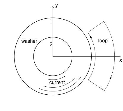
Figure 1. Current carrying washer

We take the current density to vary with the distance from the origin and to be heavily weighted toward the outer rim of the washer. We can write the planar current density explicitly as

(3.1) $${\bf J}({\bf x})=\lambda(r)\Big{(}-{\bf i}\sin\phi+{\bf j}\cos\phi\Big{)}\ \ \text{when}\ \ \ {\bf x}=(r\cos\phi,r\sin\phi,0).$$

$\lambda(r)$ is the profile of the current strength as one moves from the inner rim at $r=1/2$ to the outer rim at $r=1$. By this we mean that $\lambda(r)dr$ is the total current passing through a small radial interval $dr$ at distance $r$. We will take

(3.2) $$\lambda(r)=\frac{1}{(1-r)(\log\frac{1}{1-r})^{2}},\ \ \ 1/2\leq r<1$$

The intensity of current is therefore quite large near the outer rim. But the total current circulating around the washer is $\int_{1/2}^{1}\lambda(r)dr$, which is finite. The magnetic potential produced by the current is given by ${\bf A}=(-\Delta)^{-1}{\bf J}$. Thus

$$4\pi{\bf A}({\bf x}) =\int_{wash}\frac{{\bf J}({\bf x}^{\prime})}{|{\bf x}-{\bf x}^{\prime}|}d^{2}{\bf x}^{\prime}$$

(3.3) $$=\int_{1/2}^{1}dr\lambda(r)\int_{-\pi}^{\pi}\frac{-{\bf i}\sin\phi+{\bf j}\cos\phi}{|{\bf x}-(r\cos\phi,r\sin\phi,0)|}d\phi$$

The energy of this field is given by (See e.g. [Jac, Equ. 5.153].)

(3.4) $$W=\int_{wash}\int_{wash}\frac{{\bf J}({\bf x})\cdot{\bf J}({\bf x}^{\prime})}{|{\bf x}-{\bf x}^{\prime}|}d^{2}{\bf x}d^{2}{\bf x}^{\prime}$$

where $\int_{wash}$ means the two dimensional integral over the washer. This is equivalent to the $H_{1}$ norm of ${\bf A}$ because $\|{\bf A}\|_{H_{1}}^{2}=\int_{\mathbb{R}^{3}}\sum_{j=1}^{3}\partial_{j}{\bf A}\cdot\partial_{j}{\bf A}d^{3}x=(-\Delta{\bf A},{\bf A})=({\bf J},(-\Delta)^{-1}{\bf J})$.

Theorem 3.1.

1$)$ The gauge potential ${\bf A}$ has finite energy.

2$)$ There are piecewise smooth curves of finite length in the $x,y$ plane through which the magnetic flux is infinite. In particular the holonomy (Wilson loop) $W_{C}({{\bf A}})=e^{i\infty}$ is undefined for such a curve $C$.

Proof.

To bound the energy (3.4) take ${\bf x}=(r\cos\phi,r\sin\phi,0)$ and ${\bf x}^{\prime}=(r^{\prime}\cos\phi^{\prime},r^{\prime}\sin\phi^{\prime},0)$ in (3.4). Then $|{\bf x}-{\bf x}^{\prime}|^{2}=(r\cos\phi-r^{\prime}\cos\phi^{\prime})^{2}+(r\sin\phi-r^{\prime}\sin\phi^{\prime})^{2}=r^{2}+(r^{\prime})^{2}-2rr^{\prime}\cos(\phi-\phi^{\prime})=(r-r^{\prime})^{2}+2rr^{\prime}(1-\cos(\phi-\phi^{\prime}))$ and ${\bf J}({\bf x})\cdot{\bf J}({\bf x}^{\prime})=\lambda(r)\lambda(r^{\prime})(-{\bf i}\sin\phi+{\bf j}\cos\phi)\cdot(-{\bf i}\sin\phi^{\prime}+{\bf j}\cos\phi^{\prime})=\lambda(r)\lambda(r^{\prime})\cos(\phi-\phi^{\prime})$. Hence

$$W =\int_{1/2}^{1}\int_{1/2}^{1}drdr^{\prime}\lambda(r)\lambda(r^{\prime})\int_{-\pi}^{\pi}\int_{-\pi}^{\pi}\frac{\cos(\phi-\phi^{\prime})\ d\phi d\phi^{\prime}}{\Big{(}(r-r^{\prime})^{2}+2rr^{\prime}(1-\cos(\phi-\phi^{\prime}))\Big{)}^{1/2}}$$

(3.5) $$=2\pi\int_{1/2}^{1}\int_{1/2}^{1}drdr^{\prime}\lambda(r)\lambda(r^{\prime})\int_{-\pi}^{\pi}\frac{\cos\theta\ d\theta}{\Big{(}(r-r^{\prime})^{2}+2rr^{\prime}(1-\cos\theta)\Big{)}^{1/2}}.$$

Since $\lambda(r)$ has singular behavior near $r=1$ we will need to bound the $\theta$ integral above to prove finite energy. We will also need a lower bound later to prove that ${\bf A}({\bf x})$ is unbounded. For these purposes we will show in Section 3.1.1 that there are strictly positive constants $c_{1},c_{2},C_{1},C_{2}$ such that

(3.6) $$c_{1}+c_{2}\log\frac{1}{u} \leq\int_{-\pi/4}^{\pi/4}\frac{\cos\theta}{\Big{(}u^{2}+2v^{2}(1-\cos\theta)\Big{)}^{1/2}}d\theta\leq C_{1}+C_{2}\log\frac{1}{u}$$

(3.7) $$\text{for}\ \ 0<u<1\ \ \text{and}\ \ 1/2\leq v\leq 2$$

Now let $u=|r-r^{\prime}|$ and $v=(rr^{\prime})^{1/2}$. Then (3.7) is satisfied for all $r$ and $r^{\prime}$ entering the integrals in (3.5). The contribution to the $\theta$ integral in (3.5) from $|\theta|\geq\pi/4$ is a bounded function of $r$ and $r^{\prime}$ and since $\lambda(r)$ is integrable the contribution to (3.5) from $|\theta|\geq\pi/4$ is finite. In view of the second inequality in (3.6) it suffices therefore to show that

(3.8) $$\int_{1/2}^{1}dr\int_{1/2}^{1}dr^{\prime}\lambda(r)\lambda(r^{\prime})\log\frac{1}{|r-r^{\prime}|}<\infty.$$

Since the possibly non-integrable singularity is near $r=r^{\prime}=1$ it will be more perspicuous to change variables to $s=1-r$ and $s^{\prime}=1-r^{\prime}$. Thus we need to show that

(3.9) $$\int_{0}^{1/2}\int_{0}^{1/2}\mu(s)\mu(s^{\prime})\log\frac{1}{|s-s^{\prime}|}dsds^{\prime}<\infty$$

when $\mu(s)=(s(\log s)^{2})^{-1}$. The value of this double integral over the two triangles $s\leq s^{\prime}$ and $s^{\prime}\leq s$ is the same. So it suffices to show that one of them is finite. In fact we will show that

(3.10) $$\int_{0}^{s^{\prime}}\mu(s)\log\frac{1}{|s-s^{\prime}|}ds$$

is bounded for $0\leq s^{\prime}\leq 1/2$, which will prove (3.9) because $\mu(s^{\prime})$ is integrable.

Let $c=s^{\prime}/2$. Now $\log\frac{1}{s^{\prime}-s}$ is an increasing function of $s$ on $(0,c)$ while $\mu(s)$ is a decreasing function of $s$ on $(c,s^{\prime})$. Hence

$$\int_{0}^{s^{\prime}}\mu(s)\log\frac{1}{s^{\prime}-s}ds=\int_{0}^{c}\mu(s)\log\frac{1}{s^{\prime}-s}ds+\int_{c}^{s^{\prime}}\mu(s)\log\frac{1}{s^{\prime}-s}ds$$

(3.11) $$\leq\log\frac{1}{s^{\prime}-c}\int_{0}^{c}\mu(s)ds+\mu(c)\int_{c}^{s^{\prime}}\log\frac{1}{s^{\prime}-s}ds$$

Both integrals can be done explicitly. One finds $\int_{0}^{c}\mu(s)ds=(\log(c^{-1}))^{-1}=(\log(2/s^{\prime}))^{-1}$ and $\int_{c}^{s^{\prime}}\log\frac{1}{s^{\prime}-s}ds=(s^{\prime}/2)(1+\log(2/s^{\prime}))$. Hence the right side of (3.11) equals

$$\Big{(}\log\frac{2}{s^{\prime}}\Big{)}\frac{1}{\log\frac{2}{s^{\prime}}}+\frac{1}{(s^{\prime}/2)(\log\frac{2}{s^{\prime}})^{2}}\cdot(s^{\prime}/2)\Big{(}1+\log\frac{2}{s^{\prime}}\Big{)}=1+\frac{1+\log\frac{2}{s^{\prime}}}{(\log\frac{2}{s^{\prime}})^{2}},$$

which is bounded on $0<s^{\prime}\leq 1/2$. This proves Part 1) of Theorem 3.1.

For Part 2 we need to understand the behavior of the magnetic potential ${\bf A}({\bf x})$ as ${\bf x}$ approaches the outer rim of the washer. Because of the cylindrical symmetry it will suffice to do this when ${\bf x}$ lies in the $x,z$ plane. In fact it suffices to consider just ${\bf x}=(x_{1},0,x_{3})$ with $x_{1}\geq 0$. The distance from ${\bf x}$ to a current element is $|{\bf x}-(r\cos\phi,r\sin\phi,0)|^{2}=(x_{1}-r\cos\phi)^{2}+r^{2}\sin^{2}\phi+x_{3}^{2}=x_{1}^{2}+x_{3}^{2}+r^{2}-2x_{1}r\cos\phi=(x_{1}-r)^{2}+x_{3}^{2}+2x_{1}r(1-\cos\phi)$. Inserting this into (3.3) we see that the denominator is an even function of $\phi$. The contribution of ${\bf i}\sin\phi$ in the integral is therefore zero. Hence

(3.12) $$4\pi{{\bf A}}({\bf x})={\bf j}\int_{1/2}^{1}dr\lambda(r)\int_{-\pi}^{\pi}\frac{\cos\phi}{\Big{(}(x_{1}-r)^{2}+x_{3}^{2}+2x_{1}r(1-\cos\phi)\Big{)}^{1/2}}d\phi$$

for ${\bf x}$ in the $x,z$ plane. From the cylindrical symmetry we see that ${\bf A}({\bf x})$ is horizontal for all ${\bf x}\in\mathbb{R}^{3}$ and in fact is tangent to the horizontal circle which is centered on the $z$ axis and passes through ${\bf x}$. (On the $z$ axis ${\bf A}({\bf x})$ is zero, as one sees by putting $x_{1}=0$ in (3.12).)

Of course ${\bf A}$ is a smooth function on the complement of the closed washer because the denominator in (3.3) is locally bounded away from zero there. We need only focus attention on the behavior of ${\bf A}({\bf x})$ for ${\bf x}$ in a small neighborhood of $(1,0,0)$ in the $x,z$ plane. For such ${\bf x}$ the contribution to the integral from points in the washer where $|\phi|\geq\pi/4$ produces a smooth function of $x_{1},x_{3}$ for $x_{1}>0$. We therefore need only to analyze the behavior of the function $f$ defined by

(3.13) $$f(x_{1},x_{3})=\int_{1/2}^{1}dr\lambda(r)\int_{|\phi|\leq\pi/4}\frac{\cos\phi\ d\phi}{\Big{(}(x_{1}-r)^{2}+x_{3}^{2}+2x_{1}r(1-\cos\phi)\Big{)}^{1/2}}.$$

The first inequality in (3.6) will give a lower bound on this integral just outside the outer rim of the washer as follows. Suppose that $1\leq x_{1}\leq 5/4$ and $|x_{3}|\leq 1/2$. Let $u^{2}=(x_{1}-r)^{2}+x_{3}^{2}$ and $v^{2}=x_{1}r$. The reader can verify that (3.7) is satisfied. Hence

(3.14) $$f(x_{1},x_{3})\geq\int_{1/2}^{1}\lambda(r)(c_{1}+c_{2}\log\frac{1}{u})dr.$$

If $x_{1}\downarrow 1$ and $|x_{3}|\downarrow 0$ then $u\downarrow 1-r$ and the monotone convergence theorem shows that, for some finite constant $C_{6}$, one has

$$\liminf_{x_{1}\downarrow 0\ |x_{3}|\downarrow 0}f(x_{1},x_{3}) \geq c_{2}\int_{1/2}^{1}dr\lambda(r)\log\frac{1}{1-r}+C_{6}$$

$$=c_{2}\int_{1/2}^{1}dr\frac{1}{(1-r)(\log\frac{1}{1-r})^{2}}\log\frac{1}{1-r}+C_{6}$$

(3.15) $$=\infty.$$

Therefore ${\bf A}({\bf x})\cdot{\bf j}$ is infinite at the point $(1,0,0)$ and also goes to $\infty$ as ${\bf x}\rightarrow(1,0,0)$ in the $x,z$ plane.

Consider now the loop shown in Figure 1. It is given by a closed curve $C$ lying in the $x,y$ plane and forming the boundary of an annular sector centered at the origin and whose inner radius is one. In Figure 1 the curve is shown separated from the rim of the washer for clarity. But we are interested in the circumstance in which the inner circle of the annular sector coincides with a portion of the outer rim of the current carrying washer. The outer circle segment of $C$ is concentric with the inner one and is joined to it by radial lines. Since ${\bf A}$ is tangential to the outer rim of the washer it is also tangential to the inner circle of $C$. However this tangential component of ${\bf A}$ is infinite, as we have seen. Thus the integral of ${\bf A}$ along the inner circle of $C$ is infinite. The integral of ${\bf A}$ along the two radial lines is zero because ${\bf A}$ is perpendicular to these radial lines. The integral of ${\bf A}$ along the outer circle is finite because ${\bf A}$ is smooth in the vicinity of the outer circle. Thus $\int_{C}{\bf A}({\bf x})\cdot d{\bf x}=\infty$. This proves Part 2) of Theorem 3.1.

There is another sense in which this loop integral is infinite: keep the outer circle of the curve $C$ fixed and shift the inner circle away from the outer rim of the washer by a small amount, say $\epsilon>0$, as is shown in Figure 1. For this curve $C_{\epsilon}$ the contour integral $\int_{C_{\epsilon}}{\bf A}({\bf x})\cdot dx$ is finite, but increases to infinity as $\epsilon\downarrow 0$ because, as (3.15) shows, for $x_{3}=0$ the tangential component of ${\bf A}({\bf x})$ increases to $\infty$ as $x_{1}\downarrow 1$. In particular, by Stokes’ theorem, the magnetic flux through the planar surface bounded by $C_{\epsilon}$ increases to $\infty$ as $\epsilon\downarrow 0$. (The right hand rule also shows that the magnetic field $B$ points downward everywhere on the ring.) ∎

Remark 3.2.

Trace theorems assert that a function lying in a Sobolev space $H_{s}$ over a manifold will, upon restriction to a co-dimension one submanifold $N$, lie in $H_{s-(1/2)}(N)$. This theorem notoriously breaks down if $s=1/2$. In our case the magnetic field ${\bf A}$ lies in $H_{1}(\mathbb{R}^{3})$ and therefore restricts to a function in $H_{1/2}(N)$ for any reasonable surface $N$. One can try to restrict it once more to a curve $C$ contained in $N$ and ask what properties the restriction to $C$ has. Since $s$ is now equal to $1/2$ the trace theorem breaks down. One can not infer from it that the restriction to the curve $C$ is an almost everywhere finite function. Our example shows that the very worst can happen: the restriction of the magnetic field to an arc of the outer rim of the washer is identically infinite. For further discussion of trace theorems see [LM, Theorem 9.5] and [EL].

3.1.1. Upper and lower bounds for an integral

Lemma 3.3.

Let $0<\theta_{0}<\pi/2$ and let $a^{2}=(\sin\theta_{0})/\theta_{0}$ with $a>0$. Then, for $u>0$ and $v>0$, there holds

(3.16) $$\frac{1}{v}\log(1+\frac{v\theta_{0}}{u})\leq\int_{0}^{\theta_{0}}\frac{1}{\Big{(}u^{2}+2v^{2}(1-\cos\theta)\Big{)}^{1/2}}d\theta\leq\frac{\sqrt{2}}{va}\log(1+\frac{va\theta_{0}}{u}).$$

In particular (3.6) holds.

Proof.

For $s\geq 0$ the inequalities $1+s^{2}\leq(1+s)^{2}\leq 2(1+s^{2})$ imply that

(3.17) $$\int_{0}^{b}(1+s^{2})^{-1/2}ds\geq\log(1+b)\geq 2^{-1/2}\int_{0}^{b}(1+s^{2})^{-1/2}ds\ \text{for}\ b>0.$$

Since $a^{2}$ is the slope of a line segment lying below $\sin(\cdot)$, integration gives $a^{2}\theta^{2}\leq 2(1-\cos\theta)\leq\theta^{2}$ for $0\leq\theta\leq\theta_{0}$. Hence

$$\int_{0}^{\theta_{0}}\frac{d\theta}{\Big{(}u^{2}+v^{2}a^{2}\theta^{2}\Big{)}^{1/2}}\geq\int_{0}^{\theta_{0}}\frac{d\theta}{\Big{(}u^{2}+2v^{2}(1-\cos\theta)\Big{)}^{1/2}}\geq\int_{0}^{\theta_{0}}\frac{d\theta}{\Big{(}u^{2}+v^{2}\theta^{2}\Big{)}^{1/2}}$$

Change variables in the left-most integral to $s=(va/u)\theta$ to find $(va)^{-1}\int_{0}^{va\theta_{0}/u}(1+s^{2})^{-1/2}ds$, which, by (3.17), is at most $(va)^{-1}\sqrt{2}\log(1+(va\theta_{0}/u))$. The other half of (3.16) follows similarly.

For the proof of (3.6) we can ignore the factor $\cos\theta$ in the numerator of (3.6) because it is bounded and bounded away from zero on $[-\pi/4,\pi/4]$. We are assuming now that $1/2\leq v\leq 2$, from which it follows that the left side of (3.16) dominates the left side of (3.6) for some constants $c_{1},c_{2}$ and for all $u\in(0,1)$. Moreover, since $va\pi/4\leq 2$, the right side of (3.16) is at most $(2\sqrt{2}/a)\log(1+(2/u))\leq(4\sqrt{2}/a)\log(2/u)$ because $\log(1+x)\leq 2\log x$ when $x\geq 2$. ∎

3.2. From loops to paths

Notation 3.4.

Let $M$ be the closure of a bounded open set in $\mathbb{R}^{3}$ with smooth convex boundary. Denote by $\Gamma$ the set of piecewise $C^{1}$ functions from $[0,1]$ into $M^{int}$. If $\gamma$ and $\mu$ are two elements of $\Gamma$ such that $\gamma(1)=\mu(0)$ then their concatenation $\gamma\mu$ is defined by

(3.18) $$(\gamma\mu)(s)=\begin{cases}\gamma(2s),&0\leq s\leq 1/2\\ \mu(2s-1),&1/2\leq s\leq 1.\end{cases}$$

The curve $\gamma\mu$ is clearly again in $\Gamma$. The inverse path is defined as usual by $\gamma^{-1}(s)=\gamma(1-s),0\leq s\leq 1$. The path $\gamma\gamma^{-1}$ retraces itself.

By a parallel transport system in the bundle ${\mathcal{V}}\times M\rightarrow M$ we mean a map $\Gamma\ni\gamma\mapsto//_{\gamma}\in End\ {\mathcal{V}}$ such that

i) $//_{\gamma\circ\phi}=//_{\gamma}$ for any homeomorphism $\phi:[0,1]\rightarrow[0,1]$, which, together with its inverse, is piecewise $C^{1}$,

ii) $//_{\gamma\mu}=//_{\gamma}\ \ //_{\mu}$,

iii) $//_{\gamma\gamma^{-1}}=I_{\mathcal{V}}$.

Taking $\epsilon_{0}$ to be the trivial curve, $\epsilon_{0}(s)\equiv x_{1}$, it follows from ii) and iii) that $//_{\epsilon_{0}}=I$ and $(//_{\gamma})^{-1}=//_{\gamma^{-1}}$.

Under further technical assumptions such a parallel transport system always comes from a connection on the bundle ${\mathcal{V}}\times M\rightarrow M$. This has been discussed for example in [Po, Theorem 2.28].

We are going to show that, for a solution $A(\cdot)$ to the Yang-Mills heat equation, and for any sequence $t_{k}$ going to infinity, the parallel transport operators $//_{\gamma}^{A(t_{k})}$ converge to such a parallel transport system after suitable gauge transformations.

Choose a point $x_{0}\in M^{int}$ and denote the set of loops at $x_{0}$ by

(3.19) $$\Gamma_{0}=\{\gamma\in\Gamma:\gamma(0)=\gamma(1)=x_{0}\}.$$

A parallel transport system can be recovered, up to gauge transformation, from its restriction to $\Gamma_{0}$ by choosing a homotopy of $M$ with $x_{0}$. The well known procedure for doing this will be described in the following algebraic lemma.

Let $X$ be a manifold and let $x_{0}$ be a point in $X$. By a piecewise $C^{1}$ homotopy of $X$ with $\{x_{0}\}$ we mean a continuous map $h:[0,1]\times X\rightarrow X$ with $h(0,x)=x_{0}$, $h(1,x)=x$, and, for all $x\in X$, the curve $s\mapsto h_{x}(s):=h(s,x)$ is piecewise $C^{1}$. We will assume also that $h(s,x_{0})=x_{0}$ for all $s\in[0,1]$. Our limit results can easily be extended to non-contractible manifolds, but the analytic idea is already well illustrated in the contractible case, to which we will restrict our attention.

Lemma 3.5.

Let $X$ be a finite dimensional pathwise connected manifold. Let $x_{0}\in X$. Denote by $\Gamma$ the set of piecewise $C^{1}$ functions from $[0,1]$ into $X$ and define $\Gamma_{0}=\{\gamma\in\Gamma:\gamma(0)=\gamma(1)=x_{0}\}$. Suppose that $P:\Gamma_{0}\rightarrow End\ {\mathcal{V}}$ is a map with the following properties

$1)\ ($parametrization invariance$)$ $P(\gamma)=P(\gamma\circ\phi)$ for any piecewise $C^{1}$ homeomorphism $\phi:[0,1]\rightarrow[0,1]$ with piecewise $C^{1}$ inverse.

$2)$ $P(\gamma\mu)=P(\gamma)P(\mu)$ for all $\gamma$ and $\mu$ in $\Gamma_{0}$.

$3)$ $P(\gamma\gamma^{-1})=I_{\mathcal{V}}$ for any path $\gamma\in\Gamma$ with $\gamma(0)=x_{0}$.

Let $h:[0,1]\times X\rightarrow X$ be a piecewise $C^{1}$ homotopy of $X$ to $x_{0}$.

Then there is a unique parallel transport system $//_{\gamma},\ \gamma\in\Gamma$, which is the identity along all homotopy paths $h_{x}(\cdot)$ and agrees with $P$ on $\Gamma_{0}$.

Proof.

Suppose that $\gamma\in\Gamma$ with $\gamma(0)=x$ and $\gamma(1)=y$. Then the path $h_{x}\gamma h_{y}^{-1}$ lies in $\Gamma_{0}$. Define $//_{\gamma}=P(h_{x}\gamma h_{y}^{-1})$. If $\mu\in\Gamma$ also and $\gamma(1)=\mu(0)$ and $\mu(1)=z$ then

(3.20) $$//_{\gamma\mu}=P(h_{x}\gamma\mu h_{z}^{-1})=P((h_{x}\gamma h_{y}^{-1})(h_{y}\mu h_{z}^{-1}))=//_{\gamma}\ //_{\mu}$$

by 2). Moreover $//_{\gamma\gamma^{-1}}=P((h_{x}\gamma)(\gamma^{-1}h_{x}^{-1}))=P(h_{x}\gamma)(h_{x}\gamma)^{-1})=I_{\mathcal{V}}$ by 3). Thus items ii) and iii) are verified. Item i) is clear. Moreover $//_{h_{x}}=P(h_{x_{0}}h_{x}(h_{x})^{-1})=I_{\mathcal{V}}$. For any other parallel transport system $///$ with the stated properties one has $///_{\gamma}=///_{h_{x}}\ ///_{\gamma}\ ///_{h_{y}^{-1}}=///_{h_{x}\gamma h_{y}^{-1}}=P(h_{x}\gamma h_{y}^{-1})=//_{\gamma}$. ∎

3.3. Convergence on loops

Notation 3.6.

Let $M$ be the closure of a bounded open set in $\mathbb{R}^{3}$ with smooth convex boundary. Let $x_{0}\in M^{int}$ and define $\Gamma$ and $\Gamma_{0}$ as in Notation 3.4. In our simple setting a tangent vector to $M$ at a point $\gamma(s)$ is just a vector $u(s)\in\mathbb{R}^{3}$. We will denote by $T_{\gamma}(\Gamma)$ any piecewise $C^{1}$ function $u:[0,1]\rightarrow\mathbb{R}^{3}$. If $\gamma\in\Gamma_{0}$ then we will write $u\in T_{\gamma}(\Gamma_{0})$ if $u$ is in piecewise $C^{1}([0,1];\mathbb{R}^{3})$ and $u(0)=u(1)=0$. For $u\in T_{\gamma}(\Gamma)$ define

(3.21) $$\|u\|=\sup_{0\leq s\leq 1}|u(s)|_{\mathbb{R}^{3}}+\sup_{0\leq s\leq 1}|u^{\prime}(s)|_{\mathbb{R}^{3}}.$$

For a curve $[a,b]\ni t\rightarrow\gamma_{t}(\cdot)\in\Gamma$ we take its length to be $\int_{a}^{b}\|\partial_{t}\gamma_{t}\|dt$ as usual and define the distance $d_{1}(\gamma_{1},\gamma_{2})$ to be the infimum of lengths of curves joining $\gamma_{1}$ to $\gamma_{2}$ in the manifold $\Gamma$. $\Gamma$ and $\Gamma_{0}$ are (incomplete) metric spaces in this metric.

Definition 3.7.

For a smooth End ${\mathcal{V}}$ valued connection form $A$ on $M^{int}$ and a piecewise $C^{1}$ path $\gamma$ in $M$ the parallel transport operator along $\gamma$ is defined by the solution to the ordinary differential equation

(3.22) $$g(t)^{-1}dg(t)/dt=A\langle d\gamma(t)/dt\rangle,\ \ \ g(0)=I_{{\mathcal{V}}}.$$

We put $//_{\gamma}^{A}=g(1)$. Properties i), ii), iii) of Notation 3.4 are well known for this map.

In this section we are going to prove that for any locally bounded strong solution of the Yang-Mills heat equation satisfying Neumann or Dirichlet boundary conditions, and for any sequence of times going to infinity, there is a subsequence $t_{j}$ and gauge transforms $k_{j}$ such that the connection forms $A(t_{j})^{k_{j}}$ are smooth and the parallel transport operators $//_{\gamma}^{A(t_{j})^{k_{j}}}$ converge, as operators from ${\mathcal{V}}$ to ${\mathcal{V}}$, to a map $P$ on $\Gamma_{0}$ satisfying all the conditions listed in Lemma 3.5.

Theorem 3.8.

Suppose that $M$ is a compact convex subset of $\mathbb{R}^{3}$ with smooth boundary. Let $A(\cdot)$ be a locally bounded strong solution of the Yang-Mills heat equation (2.6) over $[0,\infty)$ satisfying Dirichlet or Neumann boundary conditions. Choose $x_{0}\in M^{int}$. Suppose that $\{t_{k}\}$ is a sequence of times going to $\infty$.

There is a function $P:\Gamma_{0}\rightarrow End\ {\mathcal{V}}$ satisfying conditions 1), 2), 3) of Lemma 3.5, a subsequence $t_{j}$ and functions $k_{j}\in W_{1}(M;K)$ such that

a$)$   $k_{j}^{-1}dk_{j}\in W_{1}(M;\mathfrak{k})$ for all $j$,

b$)$   $\alpha_{j}\equiv A(t_{j})^{k_{j}}$ is in $C^{\infty}(M;\Lambda^{1}\otimes\mathfrak{k})$ and,

c$)$ for each $\gamma\in\Gamma_{0}$ the operators $//_{\gamma}^{\alpha_{j}}$ converge to $P(\gamma)$ as $j\rightarrow\infty$.

Moreover

d$)$ $P$ is continuous on $\Gamma_{0}$ in the metric $d_{1}$.

In particular, given a piecewise $C^{1}$ homotopy of $M^{int}$ onto $x_{0}$, there is a parallel transport system on $\Gamma$ that extends $P$.

Remark 3.9.

If $\gamma$ is a closed curve in $M^{int}$ beginning at $x_{0}$, and $A$ is a smooth connection form, then for any smooth function $k:M\rightarrow K$ one has the well known identity.

(3.23) $$//_{\gamma}^{A^{k}}=k(x_{0})^{-1}(//_{\gamma}^{A})k(x_{0})$$

Consequently

(3.24) $$trace\ //_{\gamma}^{A^{k}}=trace//_{\gamma}^{A}.$$

The function $A\mapsto trace\ //_{\gamma}^{A}$ is therefore fully gauge invariant and in particular is independent of the choice of gauge transformation $k$. Theorem 3.8 implies then that there exists a sequence of times going to infinity for which the functions $\;trace//_{\gamma}^{A(t_{j})}$ converge for all piecewise $C^{1}$ loops $\gamma$ starting at $x_{0}$. One need not specify gauge transformations $k_{j}$ for this convergence.

The proof of Theorem 3.8 depends on the following lemmas.

Lemma 3.10.

Let $A(\cdot)$ be a locally bounded strong solution satisfying Dirichlet or Neumann boundary conditions and let $t_{1}>0$. Then there exists a continuous function $k:M\rightarrow K$ such that

a$)$ $k^{-1}dk\in W_{1}(M)$ and

b$)$ $\alpha\equiv A(t_{1})^{k}\in C^{\infty}(M;\Lambda^{1}\otimes\mathfrak{k})$.

Proof.

The proof depends heavily on results in [CG1]. From [CG1, Corollary 9.3] it follows that $\sup_{0<t\leq t_{1}}\|A(t)\|_{H_{1}}<\infty$. Therefore, by [CG1, Theorem 2.13] there exists $T>0$ such that, for any $t_{0}\in(0,t_{1})$, the parabolic equation

(3.25) $$(\partial/\partial t)C=-(d_{C}^{*}B_{C}+d_{C}d^{*}C),t>0,\ \ C(0)=A_{0}.$$

[CG1, Equ (2.14)] has a solution $C(\cdot)$ on the interval $[t_{0},t_{0}+T]$, with $C(t_{0})=A(t_{0})$. Pick $t_{0}\in(0,t_{1})$ such that $t_{1}<t_{0}+T$. [CG1, Corollary 8.4] then ensures that there exists a continuous function $g:M\rightarrow K$ such that $g^{-1}dg\in W_{1}$ and for which $A(t_{1})=C(t_{1})^{g}$. Since $C(t_{1})\in C^{\infty}$ we may take $k=g^{-1}$. Take note here that the equality $A(t_{1})=C(t_{1})^{g}$ relies on the uniqueness theorem, [CG1, Theorem 8.15], which is applicable to the restriction of $A(\cdot)$ to $[t_{0},t_{1}]$. ∎

Lemma 3.11.

Let $\gamma:[0,1]\rightarrow M$ be a piecewise $C^{1}$ closed curve starting at $x_{0}$. Let $u:[0,1]\rightarrow T(M)$ be a $C^{1}$ vector field along $\gamma$ for which $u(0)=u(1)=0$. That is, $u(s)\in T_{\gamma(s)}(M),0\leq s\leq 1$. Let $\alpha$ be a smooth connection form on $M$ with bounded curvature $B$. Then

(3.26) $$\|\partial_{u}//_{\gamma}^{\alpha}\|_{End\ {\mathcal{V}}}\leq\|B\|_{\infty}\sup_{0\leq s\leq 1}|u(s)|\ \ \text{Length}(\gamma).$$

Proof.

Since $u(0)=u(1)=0$ the identity [G2, Equ (2.6)] shows that

$$\Big{\|}\partial_{u}//_{\gamma}^{\alpha}\Big{\|}_{End\ {\mathcal{V}}} =\Big{\|}\int_{0}^{1}//_{\gamma|_{0}^{s}}^{\alpha}\langle B(\gamma(s)),\gamma^{\prime}(s)\wedge u(s)\rangle ds\Big{\|}_{End\ {\mathcal{V}}}$$

$$\leq\int_{0}^{1}\|//_{\gamma|_{0}^{s}}^{\alpha}\|_{End\ {\mathcal{V}}}\|B\|_{\infty}|\gamma^{\prime}(s)\wedge u(s)\rangle|_{\Lambda^{2}(\mathbb{R}^{3})}ds$$

$$\leq\|B\|_{\infty}\int_{0}^{1}|\gamma^{\prime}(s)||u(s)|ds$$

$$\leq\|B\|_{\infty}(\sup_{0\leq s\leq 1}|u(s)|)\int_{0}^{1}|\gamma^{\prime}(s)|ds,$$

which is (3.26). ∎

Proof of Theorem 3.8.

For each $\;t\geq 1$ we have constructed a gauge function $\;k(t):M\rightarrow K$ such that $\alpha(t)\equiv A(t)^{k(t)}$ is a $C^{\infty}$ connection form. Denote by $B_{\alpha}(t)$ the curvature of the connection $\alpha(t)$. Let $\gamma$ and $\eta$ be in $\Gamma_{0}$ and of length at most $L$. Define $u(s)=\gamma(s)-\eta(s)$ and let $\gamma_{\sigma}(s)=\eta(s)+\sigma u(s)$. Then $\gamma_{\sigma}$ lies in $M^{int}$ for small $\sigma$ and $\partial_{\sigma}\gamma_{\sigma}=u$. Let $b=\sup_{t\geq 1}\|B(t)\|_{\infty}$. We know that $b<\infty$ by Theorem 2.9. Since $\|B_{\alpha}(t)\|_{\infty}=\|B(t)\|_{\infty}\leq b$, Lemma 3.11 shows that

$$\|\partial_{\sigma}//_{\gamma_{\sigma}}^{\alpha(t)}\|_{End\ {\mathcal{V}}} \leq b\sup_{0\leq s\leq 1}|\gamma(s)-\eta(s)|\ \cdot\text{Length}(\gamma_{\sigma})$$

$$\leq b\sup_{0\leq s\leq 1}|\gamma(s)-\eta(s)|\ \cdot[\text{Length}(\gamma)+\text{Length}(\eta)]$$

$$\leq 2bL\sup_{0\leq s\leq 1}|\gamma(s)-\eta(s)|.$$

Hence

$$\|//_{\gamma}^{\alpha(t)}-//_{\eta}^{\alpha(t)}\|_{End\ V} \leq\int_{0}^{1}\|\partial_{\sigma}//_{\gamma_{\sigma}}^{\alpha(t)}\|_{End\ V}d\sigma$$

(3.27) $$\leq 2bL\sup_{0\leq s\leq 1}|\gamma(s)-\eta(s)|.$$

An Arzela-Ascoli type diagonalization argument shows that a pointwise bounded, equicontinuous sequence of functions on a separable metric space $S$ to a compact subset of $End\ V$ contains a subsequence that converges pointwise to a continuous function (and of course the convergence is uniform on compact subsets.) Taking the metric space to be the set $\mathcal{C}_{L}\equiv\{\gamma\in\Gamma_{0}:\text{Length}(\gamma)\leq L\}$ with the metric $d_{0}(\gamma,\eta)=\sup_{0\leq s\leq 1}|\gamma(s)-\eta(s)|$, and taking the functions to be $\{//_{\gamma}^{\alpha(t)}\}$ with ranges contained in $K\subset End\ V$, the estimate (3.27) shows that we may apply this Arzela-Ascoli argument and conclude that for any sequence of times increasing to $\infty$ there is a subsequence $t_{j}\uparrow\infty$ for which $//_{\gamma}^{\alpha(t_{j})}$ converges in operator norm for each curve $\gamma\in\mathcal{C}_{L}$. We may allow $L\uparrow\infty$ through a sequence and use diagonalization again to conclude that there is a function $P:\Gamma_{0}\rightarrow End\ V$ such that $P(\gamma)=\lim_{j\to\infty}//_{\gamma}^{\alpha(t_{j})}$ in operator norm for all $\gamma\in\Gamma_{0}$. By (3.27) $P|\mathcal{C}_{L}$ is continuous in the norm $d_{0}$ for each $L<\infty$ and therefore is continuous on $\Gamma_{0}$ in the metric $d_{1}$. The properties 1), 2), 3) of Lemma 3.5 follow from the corresponding properties of the maps $\gamma\mapsto//_{\gamma}^{\alpha(t_{j})}$. The map $P$ therefore extends, by Lemma 3.5, to a parallel transport system on paths when a piecewise $C^{1}$ homotopy of $M^{int}$ to $x_{0}$ is specified. The extension is unique in the sense given in Lemma 3.5. ∎

Acknowledgement 3.12.

N. Charalambous would like to thank the Asociación Mexicana de Cultura A.C.