Kiselman’s principle, the Dirichlet problem for the Monge–Ampère equation, and rooftop obstacle problems

Abstract

First, we obtain a new formula for Bremermann type upper envelopes, that arise frequently in convex analysis and pluripotential theory, in terms of the Legendre transform of the convex- or plurisubharmonic-envelope of the boundary data. This yields a new relation between solutions of the Dirichlet problem for the homogeneous real and complex Monge–Ampère equations and Kiselman’s minimum principle. More generally, it establishes partial regularity for a Bremermann envelope whether or not it solves the Monge–Ampère equation. Second, we prove the second order regularity of the solution of the free-boundary problem for the Laplace equation with a rooftop obstacle, based on a new a priori estimate on the size of balls that lie above the non-contact set. As an application, we prove that convex- and plurisubharmonic-envelopes of rooftop obstacles have bounded second derivatives.

1   Introduction

In this article we give a new formula for the solution of the Dirichlet problem for the homogeneous real and complex Monge–Ampère equation (HRMA/HCMA) on the product of either a convex domain and Euclidean space in the real case, or a tube domain and a Kähler manifold in the complex case. This is partly inspired by Kiselman’s minimum principle [23] and recent work of Ross–Witt-Nyström [30]. Our formula involves the convex- or plurisubharmonic-envelope of a family of functions on the Euclidean space or the manifold, and the Legendre transform on the convex domain. Consequently, one could hope to develop the existence and regularity theory for both weak and strong solutions using such a formula. In this article and in its sequels we develop this approach.

The regularity properties of the Legendre transform are classical. Thus, one is naturally led to study the regularity properties of the convex- or plurisubharmonic-envelope of a family of functions. In the case of single function with bounded second derivatives, the regularity of such envelopes was studied by Benoist–Hiriart-Urruty, Griewank–Rabier, and Kirchheim–Kristensen, [2, 16, 21] (see also [19, §X.1.5]) in the convex case, and by Berman and Berman–Demailly [3, 6] in the plurisubharmonic (psh) setting. The convex- or psh-envelope of a family of functions is, by definition, the corresponding envelope of the (pointwise) infimum of that family. However, already when the family consists of two functions, their minimum is only Lipschitz. Thus, our second goal here is to extend the aforementioned regularity results to such a setting.

The approach we take to achieve this goal is to study, more generally, the analogous subharmonic envelope. The subharmonic envelope of a ‘rooftop obstacle’ of the form $\min\{b_{0},\ldots,b_{k}\}$ is, of course, just the solution of the free-boundary problem for the Laplace equation associated to this obstacle. Our first regularity result concerning envelopes is that the solution to the free-boundary problem for the Laplace equation associated to a such a rooftop obstacle, for functions $b_{i}$ with finite $C^{2}$ norm, also has finite $C^{2}$ norm, along with an a priori estimate. Aside from basic regularity tools from the theory of free-boundary problems associated to the Laplacian, this involves a new a priori estimate on the size of a ball that lies between the rooftop and the envelope. This result stands in contrast to the results of Petrosyan–To [27] that show that the subharmonic-envelope is $C^{1,\frac{1}{2}}$ and no better for more general rootop obstacles.

Since the subharmonic-envelope always lies above both the convex- and the psh-envelope this allows us to establish the regularity of the latter envelopes as well.

An important application that makes an essential use of our results is the determination of the Mabuchi metric completion of the space of Kähler potentials, that is treated in a sequel [12].

2   Main results

Our first result concerns a new formula for the solution of the HRMA/HCMA on certain product spaces. While the real result resembles the complex result, it is not implied by it directly. Thus, we split the exposition into two (§2.1–§2.2). Our second result concerns the regularity of subharmonic-, convex-, and psh-envelopes of a ‘rooftop’ obstacle. The regularity of the latter two (§2.4) is a consequence of that of the former (§2.3). In passing, we also establish the Lipschitz regularity of the psh-envelope associated to a general Lipschitz obstacle.

2.1   A formula for the solution of the HCMA

Suppose $(M,\omega)$ is a compact, closed and connected Kähler manifold and let $K\subset\mathbb{R}^{k}$ be a bounded convex open set. Denote by $K^{\mathbb{C}}=K\times\mathbb{R}^{k}$ (considered as a subset of $\mathbb{C}^{k}$) the convex tube with base $K$. Let $\pi_{2}:K^{\mathbb{C}}\times M\to M$ denote the natural projection, and denote by $\mathrm{PSH}(K^{\mathbb{C}}\times M,\pi_{2}^{\star}\omega)$ the set of $\pi_{2}^{\star}\omega$-plurisubharmonic functions. We seek bounded $\mathbb{R}^{k}-$invariant solutions $\varphi\in L^{\infty}\cap\mathrm{PSH}(K^{\mathbb{C}}\times M,\pi_{2}^{\star}\omega)$ of the problem

$$(\pi_{2}^{\star}\omega+\sqrt{-1}\partial\bar{\partial}\varphi)^{n+k}=0\hbox{\ in $K^{\mathbb{C}}\times M$},\quad\varphi=v\hbox{\ on $\partial K^{\mathbb{C}}\times M$},$$ (1)

where the boundary data $v$ is bounded, $\mathbb{R}^{k}-$invariant and $v_{s}:=v(s,\,\cdot\,)\in\mathrm{PSH}(M,{\omega}),s\in\partial K$.

Some care is needed in defining the sense in which the boundary data is attained since the functions involved are merely bounded. In (1), by “$\varphi=v\hbox{\ on $\partial K^{\mathbb{C}}\times M$}$” we mean that for each $z\in M$ the convex function $\varphi_{z}:=\varphi(\,\cdot\,,z)$ is continuous up to the boundary of $K$ and satisfies $\varphi_{z}|_{\partial K}=v_{z}$. This choice of boundary condition implies that $v_{z}\in C^{0}(\partial K)$, and we will assume this condition on the boundary data throughout.

The study of the Dirichlet problem for the complex Monge–Ampère equation goes back to Bremermann and Bedford–Taylor [9, 1]. In particular, their results show that one should look for the solution as an upper envelope:

$$\varphi:=\sup\{w\in L^{\infty}\cap\mathrm{PSH}(K^{\mathbb{C}}\times M,\pi_{2}^{\star}\omega):\ w\textup{ is }\mathbb{R}^{k}\textup{-invariant and }w|_{\partial K^{\mathbb{C}}\times M}\leq v\},$$ (2)

generalizing the Perron method for the Laplace equation, where $w|_{\partial K^{\mathbb{C}}\times M}\leq v$ means that $\limsup_{s\to s_{0}}w(s,z)\leq v(s_{0},z)$ for all $z\in M,\ s_{0}\in\partial K$. It is not immediate, but as we will prove in Theorem 2.1, $\varphi$ is upper semi-continuous on $K^{\mathbb{C}}\times M$. Assuming this for the moment, by Bedford–Taylor’s theory $\varphi$ solves (1) (in general, further conditions are needed on $v$ in order to ensure that $\varphi|_{\partial K^{\mathbb{C}}\times M}=v$, as discussed below in Remark 3.4).

Our first result gives a different formula for expressing $\varphi$, regardless of whether $\varphi$ assumes $v$ on the boundary. It involves the psh-envelope operator solely in the $M$ variables, and the Legendre transform solely in the $K$ variables. The psh-envelope is the complex analogue of the convexification operator (or double Legendre transform) in the real setting, and is different than the upper envelope in that, roughly, it involves functions and not boundary values thereof. Given a family of upper semi-continuous bounded functions $\{f_{a}\}_{a\in{\mathcal{A}}}$ parametrized by a set ${\mathcal{A}}$, set

$$P\{f_{a}\}_{a\in{\mathcal{A}}}:=\sup\{h\in\mathrm{PSH}(M,\omega)\,:\,h(z)\leq\inf_{a\in{\mathcal{A}}}\{f_{a}(z)\},\,\forall\,z\in M\}.$$

As each $f_{b}$ is upper semi-continuous, it follows that the upper semi-continuous regularization satisfies $\textup{usc}(P\{f_{a}\}_{a\in{\mathcal{A}}})\leq f_{b}$, hence by Choquet’s lemma $\textup{usc}(P\{f_{a}\}_{a\in{\mathcal{A}}})$ is a competitor for the supremum, which in turn implies $P\{f_{a}\}_{a\in{\mathcal{A}}}=\textup{usc}(P\{f_{a}\}_{a\in{\mathcal{A}}})\in\mathrm{PSH}(M,\omega)$.

Given a function $f=f(s,z)$ on $K\times M$ (that we consider as a family of functions on $K$ parametrized by $M$), we let

$$f^{\star}(\sigma,z)=f^{\star}(\sigma):=\inf_{s\in K}[f(s,z)-\langle\sigma,s\rangle].$$ (3)

This is the negative of the usual Legendre transform solely in the $K$-variables, in particular, it maps convex functions to concave functions, and vice versa. Despite this, we also refer to it sometimes as the partial Legendre transform, and we often omit the dependence of the function on the $M$ variables in the notation. Here $\langle\,\cdot\,,\,\cdot\,\rangle$ is the pairing between $\mathbb{R}^{k}$ and its dual. Conversely, if $g=g(\sigma,z)$ is a function on $\mathbb{R}^{k}\times M$ taking values in $[-\infty,\infty)$, where $\mathbb{R}^{k}$ is considered as the dual vector space to the copy of $\mathbb{R}^{k}$ containing $K$, then

$$g^{\star}(s,z)=g^{\star}(s):=\sup_{\sigma\in\mathbb{R}^{k}}[g(\sigma,z)+\langle\sigma,s\rangle].$$ (4)

Note that $f^{\star\star}=f$ if and only if $f$ is convex, lower semicontinuous and nowhere equal to $-\infty$ (we do not allow the constant function $-\infty$), and otherwise $f^{\star\star}$ is the convexification of $f$, namely, the largest convex function majorized by $f$ [26, 15, 29].

Theorem 2.1.

Assume that $v$ is bounded, $v_{s}=v(s,\,\cdot\,)\in\mathrm{PSH}(M,{\omega})$ and $v_{z}=v(\cdot,z)\in C^{0}(\partial K)$ for all $s\in\partial K$, $z\in M$. Then $\varphi$ as defined in (2) is upper semi-continuous and

$$\varphi(h,z)=(P\{v_{s}-\langle s,\sigma\rangle\}_{s\in\partial K})^{\star}(h,z)=\sup_{\sigma\in\mathbb{R}^{k}}[P\{v_{s}-\langle s,\sigma\rangle\}_{s\in\partial K}(z)+\langle h,\sigma\rangle],\ h\in K,z\in M.$$ (5)

Equivalently, $\varphi^{\star}(\sigma,z)=\inf_{s\in K}[\varphi(s,z)-\langle\sigma,s\rangle]=P\{v_{s}-\langle s,\sigma\rangle\}_{s\in\partial K}(z)$.

To avoid confusion, we emphasize that $P\{v_{s}-\langle s,\sigma\rangle\}_{s\in\partial K}$ is not the upper envelope of a family of linear function in $\sigma$ (that would imply it is convex, which is essentially never true). Instead, the psh-envelope of this family is a global operation done for each $\sigma$ separately, and it is in fact concave in $\sigma$, as the second statement in the theorem shows.

We pause to note an important corollary of this result for the special case $K=[0,1]$, where $K^{\mathbb{C}}$ is now the strip $S:=[0,1]\times\mathbb{R}$, and (1) becomes

$$(\pi_{2}^{\star}\omega+\sqrt{-1}\partial\bar{\partial}\varphi)^{n+1}=0,\quad\varphi|_{\{i\}\times\mathbb{R}}=v_{i},\;i=0,1,$$ (6)

Corollary 2.2.

Bedford–Taylor solutions of (6) with bounded endpoints $v_{0},v_{1}\in L^{\infty}(M)$, are given by

$$\varphi(s,z)=P(v_{0},v_{1}-\sigma)^{\star}_{s}(z)=\sup_{\sigma\in\mathbb{R}}[P(v_{0},v_{1}-\sigma)(z)+s\sigma],\ s\in[0,1],\ z\in M.$$ (7)

According to Mabuchi, Semmes, and Donaldson [25, 37, 14], sufficiently regular solutions of (6) are geodesics in the Mabuchi metric on the space of Kähler potentials with respect to $\omega$. Thus, Corollary (2.2) implies that Mabuchi’s geometry is essentially determined by the understanding of upper envelopes of the form $P({v_{0}},v_{1}-\tau)$, for all $v_{0},v_{1}\in\mathrm{PSH}(M,\omega)\cap L^{\infty}(M)$ and for all $\tau\in\mathbb{R}$. We refer to the sequel [12] for applications of Corollary 2.2 in this direction, in particular, determining the metric completion of the Mabuchi metric.

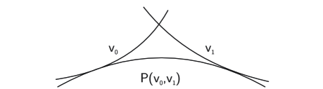
Figure 1: The barriers $v_{0},v_{1}$ and the envelope $P(v_{0},v_{1})$

2.2   A formula for the solution of the HRMA

Theorem 2.1 has a convex analogue in the setting of the HRMA. The result does not follow directly from the seemingly harder result for the HCMA. For concreteness, we only state the analogue of Corollary 2.2 in this setting, that arises in the setting of the Mabuchi metric on a toric manifold $M$. The reader is referred to [34, §2] for the relevant background concerning the HRMA and toric geometry.

For $z$ belonging to the open orbit of the complex torus $(\mathbb{C}^{n})^{\star}$ (that is dense in $M$), set $x=\hbox{\rm Re}\log z\in\mathbb{R}^{n}$. On the open orbit, $\omega=\sqrt{-1}\partial\bar{\partial}\psi_{\omega}$ with $\psi_{\omega}$ $(S^{1})^{n}$-invariant, thus consider $\psi_{\omega}$ as a function on $\mathbb{R}^{n}$. Then, the HCMA (1) reduces to the HRMA,

$$\hbox{MA}\psi(s,x)=0,\quad\hbox{on }[0,1]\times\mathbb{R}^{n},\qquad\psi_{i}(x)\equiv\psi(i,x)=\psi_{\omega}(x)+v_{i}(e^{x}),\quad i\in\{0,1\}.$$ (8)

Here, MA is the unique continuous extension of the operator $f\mapsto d\frac{\partial f}{\partial x_{1}}\wedge\cdots\wedge d\frac{\partial f}{\partial x_{n}}$ from $C^{2}(\mathbb{R}^{n})$ to the cone of convex functions on $\mathbb{R}^{n}$.

The following is a convex version of Corollary 2.2.

Proposition 2.3.

The solution of (8) with convex endpoints $\psi_{0},\psi_{1}$ is given by

$$\psi=(\min\{\psi_{0},\psi_{1}-\sigma\}^{\star\star})^{\star}=\sup_{\sigma\in\mathbb{R}}[\min\{\psi_{0},\psi_{1}-\sigma\}^{\star\star}+s\sigma].$$ (9)

Here the first (innermost) two Legendre transforms are in the $x$ variables, while the third (outermost) negative Legendre transform is in the $\sigma$ variable. Note that, strictly speaking, this result is not a consequence of Corollary 2.2, since it involves the potentially larger convex envelope (the supremum is taken over convex functions that might not come from toric potentials) and not the psh-envelope; rather, Proposition 2.3 implies Corollary 2.2 (in this symmetric setting) since it shows that the psh-envelope in this setting is attained at a ‘toric’ convex function.

This formula also has an interpretation in terms of Hamilton–Jacobi equations, in the spirit of [35], that we discuss elsewhere.

2.3   Regularity of rooftop subharmonic-envelopes

The following result plays a crucial role in our proof of the regularity of convex- and psh-envelopes of rooftop obstacles. It is of independent interest to the study of regularity of solutions to the free-boundary problem for rooftop obstacles for the Laplacian. The solution of the aforementioned free-boundary value problem is, in fact, the subharmonic-envelope of rooftop obstacles. This is a purely local result, and is stated on the open unit ball $B_{1}$ in $\mathbb{R}^{n}$ (we let $B_{R}(x_{0})$ denote the ball of radius $R$ centered at $x_{0}\in\mathbb{R}^{n}$; when $x_{0}=0$ we write $B_{R}=B_{R}(0)$). Denote by $\mathrm{SH}(B_{1})$ the set of subharmonic functions on $B_{1}$.

Theorem 2.4.

Let $b_{0},b_{1}\in C^{1,1}(B_{1})$, and let

$$b_{\operatorname{env}}:=\sup\{f\in\mathrm{SH}(B_{1})\,:\,f\leq\min\{b_{0},b_{1}\}\}.$$ (10)

Then, there exists a constant $C=C(n,\|b_{0}\|_{C^{2}(B_{1})},\|b_{1}\|_{C^{2}(B_{1})})$ such that

$$\|b_{\operatorname{env}}\|_{C^{2}(B_{1/8})}\leq C.$$

2.4   Regularity of the convex-envelope or psh-envelope of a family of functions

Given an upper semi-continuous family $\{f_{a}\}_{a\in\mathcal{A}}$ with additional regularity properties, one would like to study how much regularity is preserved by the envelope $P\{f_{a}\}_{a\in\mathcal{A}}$. Motivated by Corollary 2.2 and Proposition 2.3, we are led to study the regularity of upper envelopes of the type $P(v_{0},v_{1})$. Here, we concentrate on the case when the barriers (sometimes also called obstacles) $v_{0}$ and $v_{1}$ are rather regular. The sequel [12] treats the case when $v_{0}$ or $v_{1}$ are rather irregular in the psh setting. Already in the case of smooth convex functions, the convexification is not $C^{2}$ in general. Thus, the following results gives conditions that guarantee essentially optimal regularity. A novelty of our approach, perhaps, is that both the convex- and the psh-envelopes are handled simultaneously.

To state the results, we define the Banach space

$$C^{1\bar{1}}(M):=\{f\in L^{\infty}(M)\,:\,\Delta_{\omega}f\in L^{\infty}(M)\},$$ (11)

with associated Banach norm

$$||f||_{C^{1\bar{1}}}:=||f||_{L^{\infty}(M)}+||\Delta_{\omega}f||_{L^{\infty}(M)}.$$ (12)

If $Cf\in\mathrm{PSH}(M,\omega)$ for some $C>0$, then $f\in C^{1\bar{1}}(M)$ if and only if $\sqrt{-1}\partial\bar{\partial}f$ is a current with bounded coefficients. We also define, as usual, $C^{1,1}(M)$ to be the Banach space of functions on $M$ with finite $C^{2}(M)$ norm. One has $C^{2}(M)\subset C^{1,1}(M)\subset C^{1\bar{1}}(M)$.

Theorem 2.5.

One has the following estimates: (i) $\|P(v)\|_{C^{1}}\leq C(M,\omega,\|v\|_{C^{1}})$. (ii) $\|P(v_{0},v_{1})\|_{C^{1\bar{1}}}\leq C(M,\omega,\|v_{0}\|_{C^{1\bar{1}}},\|v_{1}\|_{C^{1\bar{1}}}).$ (iii) Suppose $[\omega_{0}]\in H^{2}(M,\mathbb{Z})$. Then, $\|P(v_{0},v_{1})\|_{C^{2}}\leq C(M,\omega,\|v_{0}\|_{C^{2}},\|v_{1}\|_{C^{2}}).$

Our convention here and below is that the constants $C$ on the right hand side of the estimates just stated may equal to $\infty$ only if the corresponding norms of $v$ or $v_{i}$ are infinite.

An analogous result can be stated for convex rooftop envelopes. For simplicity, we only state a representative result in the toric setting of Proposition 2.3.

Corollary 2.6.

Let $\psi_{0},\psi_{1}$ be as in Proposition 2.3. Then,

$$\|\min\{\psi_{0},\psi_{1}\}^{\star\star}\|_{C^{2}}\leq C(M,\omega,\|\psi_{0}\|_{C^{2}},\|\psi_{1}\|_{C^{2}}).$$

By repeated application of the formula $P(v_{0},v_{1},\ldots,v_{k})=P(v_{0},P(v_{1},\ldots,v_{k}))$, the results just stated hold also for envelopes of the type $P(v_{0},\ldots,v_{k})$.

In general, the convex- or subharonic-envelope of a Lipschitz function will be no better than Lipschitz, as shown by Kirchheim–Kristensen [21], and by Caffarelli [10, Theorem 2], respectively. Theorem 2.5 (i) is the analogous fact for psh-envelopes. The psh-envelope of a family of functions, e.g., $P(v_{0},v_{1})$ is of course the psh-envelope of the single function $\min\{v_{0},v_{1}\}$ that is in general only Lipschitz. Thus, the point of Theorem 2.5 (ii)–(iii) is that for special Lipschitz functions of the form $\min\{v_{0},\ldots,v_{k}\}$ that we refer to as rooftop functions (see Figure 1) the psh-envelope has a regularizing effect, roughly gaining a derivative.

The proof of Theorem 2.5 uses basic techniques from the theory of free boundary problems for the Laplacian, together with results of Berman [3] and Berman-Demailly [6] on upper envelopes of psh functions. Part (i) is, in fact, a simple consequence of the Lipschitz estimate of B ̵locki [8] in conjunction with the “zero temprature” approximation procedure of Berman [5]. The bulk of the proof is thus devoted to parts (ii)–(iii). The key step is to show that there exists a $C^{1,1}$ function $b$ (a ‘barrier’) along with an a priori estimate depending only on the respective norms of the $v_{i}$, such that $b$ lies below $\min\{v_{0},v_{1}\}$ but above $P(v_{0},v_{1})$. The barrier we construct is actually obtained by first constructing local subharmonic-envelopes of $v_{0}$ and $v_{1}$ on coordinate charts. This construction is mostly based on well-known techniques from the study of the free boundary Laplace equation, see, e.g., [10, 11, 28], but with one essential new ingredient, that we now describe. For a general rooftop obstacle (that is, not necessarily of the form $\min\{v_{0},v_{1}\}$) Petrosyan–To [27] show that the subharmonic-envelope is $C^{1,\frac{1}{2}}$ and no better. Yet, also in the literature on subharmonic-envelopes we were not able to find the regularization statement for rooftop obstacles of the form $\min\{v_{0},v_{1}\}$ although it might very well be known to experts. Thus, the main new technical ingredient is the estimate of Proposition 4.5 that guarantees that around each point in the set $\{v_{0}=v_{1}\}$ there exists a ball of a priori estimable size that stays away from the contact set, i.e., the set where the local subharmonic envelope equals the barrier $\min\{v_{0},v_{1}\}$. Given this estimate, the standard quadratic growth estimate carries over to our setting, and one obtains a priori estimates on $b$. Then, since the subharmonic-envelope necessarily majorizes the psh-envelope, we get $P(b)=P(v_{0},v_{1})$, to which one may apply Berman–Demailly’s results.

A regularity result of a similar nature has been recently proved by Ross–Witt-Nystrom [31] in a different setting. Namely, they study regularity of envelopes of the type $P_{[\phi]}(\psi)=\textup{usc}\big{(}\sup_{c>0}P(\phi+c,\psi)\big{)}$, where $\psi\in C^{1\bar{1}}(M)$, $\phi\in\mathrm{PSH}(M,\omega)$ is exponentially Hölder continuous and $M$ is polarized. Also, upon completing this article, we were informed by Berman that the technique of [6] can be extended to prove Theorem 2.5(iii) [4]. Perhaps the novel point in our approach, compared to such an extension, is that it also gives, in passing, a useful result concerning the obstacle problem for the Laplacian, and thus proves the regularity of the subharmonic-, convex-, and psh-envelopes, all at once.

2.5   Applications to regularity of Bremermann upper envelopes

A combination of Theorem 2.1 and Theorem 2.5 (i) gives fiberwise Lipschitz regularity of the Bremermann upper envelope $\varphi$ (2) associated to fiberwise Lipschitz boundary data. This provides an instance when one can draw conclusions about the regularity of $\varphi$ by studying first the regularity of its partial Legendre transform.

Corollary 2.7.

In the setting of Theorem 2.1, the envelope $\varphi$ satisfies

$$\|\varphi(s,\cdot)\|_{C^{1}}\leq C(M,\omega,\sup_{s\in\partial K}\|v(s,\cdot)\|_{C^{1}}),\quad\hbox{for any $s\in K$}.$$

In other words, if the boundary data is fiberwise Lipschitz, so is the envelope, and with a uniform estimate.

The novelty of this result is that it proves regularity of the envelope $\varphi$, whether or not it solves the HCMA. We are not aware of any such results in the literature. At the same time, when $\varphi$ does solve the HCMA then other techniques exist, notably B ̵locki’s Lipschitz estimate [8]. However, even then our method seems to be new in that it furnishes fiberwise Lipschitz regularity given the same on the boundary data, while B ̵locki’s estimate alone gives full Lipschitz regularity starting from full (also in the $\partial K$ directions) Lipschitz regular data. Of course, it should be stressed that we ultimately use B ̵locki’s estimate in our proof, but we do so only in the fiberwise directions.

Organization

Theorem 2.1 and Corollary 2.2 are proved in §3. The convex analogue, Proposition 2.3, is proved in §3.1. Theorem 2.5 (i) concerning Lipschitz regularity of the psh-envelope is proved in §4.1, where we also prove Corollary 2.7. Theorem 2.5 (ii)–(iii) and Corollary 2.6, concerning the regularity of second derivatives of the psh- and convex-envelopes, are proved in §4.2. Finally, the main regularity result concerning the subharmonic envelope, Theorem 2.4, is proved in §4.3.

3   The Dirichlet problem on the product of a tube domain and a manifold

Suppose that $f(s,z)$ is a convex function on $\mathbb{R}^{k}_{s}\times\mathbb{R}^{m}_{z}$. Then $\inf_{s}f(s,z)$ is either identically $-\infty$, or else a convex function on $\mathbb{R}^{m}$ [29, Theorem 5.7; p. 144],[24, Theorem 1.3.1]. If we replace “convex” with “psh” and $\mathbb{R}$ by $\mathbb{C}$ this is not true in general. A special situation in which this is true was described by Kiselman. Let us recall a local version of this result [23] (cf. [13, Theorem I.7.5]). As in §2.1, let $K\subset\mathbb{R}^{k}$ be a convex set and denote by $K^{\mathbb{C}}:=K+\sqrt{-1}\mathbb{R}^{k}\subset\mathbb{C}^{k}$ the tube domain associated to $K$. Denote by $s$ a coordinate on $K\subset\mathbb{R}^{k}$ and by $\tau:=s+\sqrt{-1}t$ a coordinate on $K^{\mathbb{C}}\subset\mathbb{C}^{k}$.

Theorem 3.1.

Let $D\subset\mathbb{C}^{n}$ be a domain. If $v\in\mathrm{PSH}(K^{\mathbb{C}}\times D)$ is such that that $v(s+\sqrt{-1}t,z)=v(s,z)$ for all $t\in\mathbb{R}^{k}$ then

$$v(z)=\inf_{\tau\in K^{\mathbb{C}}}v(\tau,z)$$ (13)

is either identically $-\infty$, or else psh on $D$.

This immediately implies the following global version. As in §2.1, we denote by $(M,\omega)$ a Kähler manifold and by $\pi_{2}:K^{\mathbb{C}}\times M\rightarrow M$, $\pi_{1}:K^{\mathbb{C}}\times M\rightarrow K^{\mathbb{C}}$ the natural projections.

Corollary 3.2.

Assume that $f\in\mathrm{PSH}(K^{\mathbb{C}}\times M,\pi_{2}^{\star}\omega)$ satisfies $f(s,z)=f(s+\sqrt{-1}t,z)$ for all $t\in\mathbb{R}^{k}$. Then $f^{\star}(\sigma,z)$, as defined in (3), satisfies $f^{\star}(\sigma,\,\cdot\,)\in\mathrm{PSH}(M,\omega)$ for each $\sigma\in\mathbb{R}^{k}$.

Proof of Theorem 2.1.

We argue that $\varphi$ is upper semi-continuous parallel with the proof of the formula

$$\varphi^{\star}(\sigma,z)=\inf_{s\in K}[\varphi(s,z)-\langle\sigma,s\rangle]=P\{v_{s}-\langle s,\sigma\rangle\}_{s\in\partial K}(z),\ \sigma\in\mathbb{R}^{k},\ z\in M.$$ (14)

To start, observe that both $\varphi(\,\cdot\,,z)$ and $(\textup{usc}\,\varphi)(\,\cdot\,,z)$ are convex and bounded functions on $K$ for each $z\in M$ (note that $\sup\textup{usc}\,\varphi=\sup\varphi$). Indeed, the former is a supremum of convex functions , where as the latter is the restriction to $K\times\{z\}$ of an $\mathbb{R}^{k}$-invariant $\omega-$psh function by Choquet’s lemma. Thus, it suffices to prove that

$$\varphi^{\star}(\sigma,z)=(\textup{usc}\,\varphi)^{\star}(\sigma,z),$$ (15)

for all $\sigma\in\mathbb{R}^{k}$ since then, by applying another partial Legendre transform it follows that $\varphi=\textup{usc}\,\varphi$. The proof of (15) will be implicit in the proof of (14) below.

Recall that by Bedford-Taylor theory [22, Theorem 1.22] the set $E=\{\varphi<\textup{usc}\,\varphi\}\subset K^{\mathbb{C}}\times M$ has capacity zero, in particular its Lebesgue measure is also zero (meaning that $\int_{E}dV_{K^{\mathbb{C}}\times M}=0$ for any smooth volume form $dV_{K^{\mathbb{C}}\times M}$ on $K^{\mathbb{C}}\times M$). As both $u$ and $\textup{usc}\,u$ are $\mathbb{R}^{k}$-invariant, $E$ is also $\mathbb{R}^{k}$-invariant with base $B\subset K\times M$ (note that $B$ is not a subset of $K$). Clearly, the Lebesgue measure of $B$ is zero. For $z\in M$ we introduce the sets

$$B_{z}=\pi_{1}(B\cap K\times\{z\})\subset K.$$

It follows that $B_{z}$ has Lebesgue measure zero for all $z\in M\setminus F$, where $F\subset M$ has Lebesgue measure zero.

Suppose $z\in M\setminus F$, we claim that in fact $B_{z}$ is empty. This follows, as the continuous convex functions $\varphi(\,\cdot\,,z)$ and $(\textup{usc}\,\varphi)(\,\cdot\,,z)$ agree on the dense set $K\setminus B_{z}$, hence they have to agree on all of $K$, hence $B_{z}$ is empty. This implies that

$$\varphi^{\star}(\sigma,z)=(\textup{usc}\,\varphi)^{\star}(\sigma,z),\quad\textup{ for all }z\in M\setminus F,\sigma\in\mathbb{R}^{k}.$$ (16)

Now, by Corollary 3.2, for each $\sigma\in\mathbb{R}^{k}$, the function $(\textup{usc }\varphi)^{\star}(\sigma,\,\cdot\,)$ belongs to $\mathrm{PSH}(M,\omega)$. Moreover, by definition of $\varphi$ we have

$$\varphi^{\star}_{\sigma}\leq\varphi_{s}-\langle\sigma,s\rangle\textup{ for all }s\in K.$$ (17)

We can in fact extend this estimate to the boundary of $\partial K$:

Claim 3.3.

For all $s\in\partial K$ and $\sigma\in\mathbb{R}^{k}$, $\varphi^{\star}(\sigma,z)\leq v_{s}(z)-\langle\sigma,s\rangle$.

Indeed, as $v_{z}\in C(\partial K)$ for all $z\in M$, it follows that $\varphi(p,z)\leq\mathcal{P}[v_{z}](p),\ p\in K$, where $\mathcal{P}[v_{z}]\in C(\overline{K})$ is the harmonic function on $K$ satisfying $\mathcal{P}[v_{z}]|_{\partial K}=v_{z}.$ This implies that $\limsup_{p\to s}\varphi_{p}(z)\leq v_{s}(z)$ for all $z\in M,\ s\in\partial K$, hence we can take the $\limsup$ of the right hand side of (17) to conclude the claim.

Thus, by (16) we also have $(\textup{usc}\,\varphi)^{\star}(\sigma,z)\leq v_{s}(z)-\langle\sigma,s\rangle$ for $z\in M\setminus F,\ s\in\partial K$. As $F$ has Lebesgue measure zero we claim that this inequality extends to all $z\in M$. This follows from the fact that $(\textup{usc}\,\varphi)^{\star}_{\sigma}$ and $v_{s}-\langle\sigma,s\rangle$ are $\omega-$psh for fixed $s\in\partial K$, hence by the sub-meanvalue property we can write:

$$(\textup{usc}\,\varphi)^{\star}_{\sigma}(z)=\lim_{r\to 0}\oint_{B(z,r)}(\textup{usc}\,\varphi)^{\star}_{\sigma}(\xi)dV(\xi)\leq\lim_{r\to 0}\oint_{B(z,r)}(v_{s}(\xi)-\langle\sigma,s\rangle)dV(\xi)=\varphi_{s}(z)-\langle\sigma,s\rangle,$$

for all $z\in M$, where $B(z,r)$ is a coordinate ball around $z$ and $dV$ is the standard Euclidean measure in local coordinates.

Thus, $(\textup{usc}\,\varphi)^{\star}(\sigma,\cdot)$ is a competitor in the definition of $P\{v_{s}-\langle s,\sigma\rangle\}_{s\in\partial K}$ concluding that

$$\varphi^{\star}(\sigma,\,\cdot\,)\leq(\hbox{usc}\,\varphi)^{\star}(\sigma,\,\cdot\,)\leq P\{v_{s}-\langle\sigma,s\rangle\}_{s\in\partial K}.$$ (18)

Conversely, let $\chi\in\mathrm{PSH}(M,\omega)$ satisfy $\chi\leq v_{a}-\langle a,\sigma\rangle$ for each ${a\in\partial K}$. We claim that $\chi\leq\varphi_{s}-\langle s,\sigma\rangle$ for every $s\in K$. Indeed, by (2),

$$\varphi_{s}-\langle s,\sigma\rangle=\sup\{w_{s}-\langle s,\sigma\rangle\in L^{\infty}\cap\mathrm{PSH}(K^{\mathbb{C}}\times M,\pi_{2}^{\star}\omega):(w-\langle s,\sigma\rangle)|_{\partial K^{\mathbb{C}}}\leq v-\langle s,\sigma\rangle\},$$

so $\chi$ is a competitor in this last supremum, proving the claim. Now, taking the infimum over all $s\in K$ it follows that

$$\varphi^{\star}(\sigma,\cdot)\geq P\{v_{s}-\langle s,\sigma\rangle\}_{s\in\partial K}.$$ (19)

Putting together (18) and (19) the identities (14) and (15) follow, proving that $u$ is upper semi-continuous. ∎

Remark 3.4.

To guarantee that $\varphi$ defined by (2) is an actual solution of (1), one can, e.g., assume that there exists a subsolution, by which we mean an $\mathbb{R}^{k}$-invariant $w\in L^{\infty}\cap\mathrm{PSH}(K^{\mathbb{C}}\times M,\pi_{2}^{\star}\omega)$ satisfying $w|_{\partial K^{\mathbb{C}}}=v$. In fact, if such a subsolution exists, then $w_{z}\leq\varphi_{z}$, implying that $\varphi_{z}|_{\partial K}$ lies above the boundary data. On the other hand, $\varphi_{z}\leq\mathcal{P}[v_{z}]$, where $\mathcal{P}[v_{z}]\in C(\overline{K})$ is the harmonic function on $K$ satisfying $\mathcal{P}[v_{z}]|_{\partial K}=v_{z}.$ Thus, $\varphi_{z}|_{\partial K}$ also lies below the boundary data. In sum, $\varphi|_{\partial K^{\mathbb{C}}}=v$.

Providing a subsolution is often possible given special properties of $K$ or the boundary data $v$. An instance of this is the situation described in Corollary 2.2:

Proof of Corollary 2.2.

By Theorem 2.1, all one needs to verify is that $\varphi$, as defined in (2), satisfies $\varphi|_{\{i\}\times\mathbb{R}}=v_{i},\;i=0,1$. Formula (7) follows then from (5). However, by an observation of Berndtsson [7] we have that the function $w(s,z)=\max\{v_{0}(z)-As,v_{1}(z)+A(1-s)\}\in PSH(K^{\mathbb{C}}\times M,\pi_{2}^{*}\omega)$ satisfies $\psi|_{\{i\}\times\mathbb{R}}=v_{i},\;i=0,1,$ where $A=\max\{\|v_{0}\|_{L^{\infty}},\|v_{1}\|_{L^{\infty}}\}.$ Hence, $w$ is a subsolution in the sense of Remark 3.4. ∎

We remark in passing that the general argument to prove upper semicontinuity given in Theorem 2.1 can be avoided in the special setting of Corollary 2.2 (i.e., when $K=[0,1]$). Indeed, by convexity in $s$, $\varphi(s,z)\leq sv_{0}(z)+(1-s)v_{1}(z)$ for all $(s,z)\in[0,1]\times M$, thus also $\textup{usc}\,\varphi$ satisfies the same inequality. This last estimate in turn implies that $\textup{usc}\,\varphi$ is a candidate in the supremum defining $\varphi$, thus $\textup{usc}\,\varphi=\varphi$ (cf. [7]).

3.1   A convex version for the HRMA

In this subsection we prove the a version of Corollary 2.2 for the homogeneous real Monge–Ampère (HRMA) equation. While a proof of Proposition 2.3 and even its generalization to higher dimensional $K$ can be given along very similar lines to the proof of Theorem 2.1, we give below a somewhat different argument.

Proof of Proposition 2.3.

As observed by Semmes [36, 37], the HRMA is linearized by the partial Legendre transform in the $\mathbb{R}^{n}$ variables. Thus, the solution to the HRMA is given by

$$\psi(s,x)=((1-s)\psi_{0}^{\star}+s\psi_{1}^{\star})^{\star}(x),$$ (20)

where $\psi_{i}^{\star}(y)=\sup_{y\in\mathbb{R}^{n}}[\langle x,y\rangle-\psi_{i}(y)]$. As is well-known, this is equal to the infimal convolution of $\psi_{0}$ and $\psi_{1}$ [29, Theorem 38.2],

$$\inf_{\{x_{0},x_{1}\in\mathbb{R}^{n}\,:\,(1-s)x_{0}+sx_{1}=x\}}[(1-s)\psi_{0}(x_{0})+s\psi_{1}(x_{1})].$$ (21)

This also follows directly from the fact that $\psi$ solves the HRMA, since by [35] a solution of the HRMA solves a Hamilton–Jacobi equation, and (21) is just the Hopf–Lax formula in that setting. Now, we take the negative Legendre transform of (20) in $s$ to obtain,

$$\psi^{\star}_{x}(\sigma) =\min_{s\in[0,1]}\Big{[}\inf_{\{x_{0},x_{1}\in\mathbb{R}^{n}\,:\,(1-s)x_{0}+sx_{1}=x\}}[(1-s)\psi_{0}(x_{0})+s\psi_{1}(x_{1})]-s\sigma\Big{]}$$

$$=\min_{s\in[0,1]}\Big{[}\inf_{\{x_{0},x_{1}\in\mathbb{R}^{n}\,:\,(1-s)x_{0}+sx_{1}=x\}}[(1-s)\psi_{0}(x_{0})+s(\psi_{1}(x_{1})-\sigma)]\Big{]}.$$

Now we will show that this last expression is equal to

$$\sup\{v\,:\,v\hbox{\ is convex on }\mathbb{R}^{n}\hbox{\ and $v\leq\min\{\psi_{0},\psi_{1}-\sigma\}$}\}=\min\{\psi_{0},\psi_{1}-\sigma\}^{\star\star}.$$ (22)

Fix $x\in\mathbb{R}^{n}$, and let $s\in[0,1]$ and $x_{0},x_{1}\in\mathbb{R}^{n}$ be such that $(1-s)x_{0}+sx_{1}=x$. Let $v$ be a convex function satisfying $v\leq\min\{\psi_{0},\psi_{1}-\sigma\}$. Then,

$$(1-s)\psi_{0}(x_{0})+s(\psi_{1}(x_{1})-\sigma)\geq(1-s)v(x_{0})+sv(x_{1})\geq v(x),$$

by convexity of $v$. Thus, $\psi^{\star}_{x}(\sigma)\geq\min\{\psi_{0},\psi_{1}-\sigma\}^{\star\star}$.

Conversely, the expression (21) is a convex function jointly in $s$ and $x$ (since it is evidently convex in $x$ by (20) and it solves the HRMA in all variables). By the minimum principle for convex functions then $\psi^{\star}_{x}(\sigma)$ is convex in $x$. By the definition of the negative Legendre transform in $s$, $\psi^{\star}_{x}(\sigma)\leq\min_{s\in\{0,1\}}[\psi_{s}(x)-s\sigma]=\min\{\psi_{0}(x),\psi_{1}-\sigma\}$. Thus, $\psi^{\star}_{x}(\sigma)$ is a competitor in the left hand side of (22). Hence, $\psi^{\star}_{x}(\sigma)\leq\min\{\psi_{0},\psi_{1}-\sigma\}^{\star\star}$. ∎

4   Regularity of upper envelopes of families

The bulk of this section is devoted to the proof of Theorem 2.5 (ii)–(iii) and Corollary 2.6 that establish the regularity of psh- and convex-envelopes envlopes associated to obstacles of the form $\min\{b_{0},b_{1}\}$, that we refer to as ‘rooftop’ envelopes (see Figure 1). However, we begin by first proving the Lipschitz regularity of psh-envelopes (Theorem 2.5 (i)).

4.1   Lipschitz regularity of psh-envelopes

Let $v\in C^{\infty}(M)$. Berman developed the following approach for constructing $P(v)$, generalizing a related construction for obtaining “short-time” solutions to the Ricci continuity method, introduced in [32], in turn based on a result of Wu [38] (a new approach to which has been given in [20, §9], see [33, §6.3] for an exposition of these matters). For $\beta$ positive and sufficiently large one considers the equations

$$(\omega+\sqrt{-1}\partial\bar{\partial}u_{\beta})^{n}=e^{\beta(u_{\beta}-v)}\omega^{n}.$$ (23)

By the classical work of Aubin and Yau, (23) admits a smooth solution $u_{\beta}$. Berman proves that, as $\beta$ tends to infinity, $u_{\beta}$ converges to $P(v)$ uniformly, and that, moreover, there is an a priori Laplacian estimate in this setting [5]. In this section we observe that, as expected, also an a priori Lipschitz estimate holds, by directly applying B ̵locki’s estimate. In other words, we prove Theorem 2.5 (i). The proof will show that the constant in Theorem 2.5 (i) depends on a lower bound of the bisectional curvature of $(M,\omega)$ and on $||v||_{C^{1}(M)}$. We claim no originality in the proof below.

Proof of Theorem 2.5 (i).

It suffices, by a standard approximation procedure, to assume that $v$ is smooth. For simplicity of notation, we will often denote $u_{\beta}$ by just $u$. The argument follows [8, Theorem 1] very closely. Let $B^{\prime}$ be some sufficiently large positive constant to be fixed later. Let $C_{0}:=\sup_{\beta>2}||u_{\beta}||_{C^{0}}+1$. Let $\phi:M\to\mathbb{R}$ be the following function:

$$\phi:=\log|\partial u|_{\omega}^{2}-\gamma(u),$$

where $\gamma:[-C_{0},C_{0}]\to\mathbb{R}$ is a smooth non-decreasing function to be fixed later. Since $\|u\|_{C^{0}}\leq C(M,\|v\|_{C^{0}}),$ independently of $\beta$ [5], $\gamma$ is thus defined on some fixed finite interval.

Suppose $\phi$ attains its maximum at $p\in M$. Let $z=(z_{1},\ldots,z_{n})$ denote holomorphic normal coordinates around this point. Let $g$ denote a local potential for $\omega$ in this chart, i.e., $\sqrt{-1}\partial\bar{\partial}g=\omega$. Set $h:=g+u$. We can additionally suppose that $\sqrt{-1}\partial\bar{\partial}u(p)$ is diagonal in our coordinates. Since all our local calculations will be carried out at the point $p$ we omit the dependence on this point from the subsequent computations. Let

$$\alpha:=|\partial u|_{\omega}^{2}.$$

Thus,

$$0=\frac{\partial}{\partial z_{j}}\phi=\phi_{j}=\frac{\alpha_{j}}{\alpha}-\gamma^{\prime}(u)u_{j},\quad j=1,\ldots,n,$$ (24)

and so (omitting from now and on symbols for summation that can be understood from the context),

$$0\geq\Delta_{\omega_{u}}\phi=\frac{\phi_{k\bar{k}}}{h_{k\bar{k}}}=\frac{1}{h_{k\bar{k}}}\Big{(}\frac{\alpha_{k\bar{k}}}{\alpha}-\frac{|\alpha_{k}|^{2}}{\alpha^{2}}-\gamma^{\prime}u_{k\bar{k}}-\gamma^{\prime\prime}\alpha\Big{)}=\frac{1}{h_{k\bar{k}}}\Big{(}\frac{\alpha_{k\bar{k}}}{\alpha}-\gamma^{\prime}u_{k\bar{k}}-(\gamma^{\prime\prime}+\gamma^{\prime 2})\alpha\Big{)},$$ (25)

The next formula holds for each fixed $k=1,\ldots,n$ (no summation)

$$\alpha_{k\bar{k}}=2\hbox{\rm Re}\ u_{jk\bar{k}}u_{\bar{j}}+|u_{jk}|^{2}+|u_{j\bar{k}}|^{2}-u_{j}g_{j\bar{l}k\bar{k}}u_{\bar{l}}\geq 2\hbox{\rm Re}\ u_{jk\bar{k}}u_{\bar{j}}+|u_{jk}|^{2}-B\alpha,$$ (26)

whenever $-B$ is a lower bound for the bisectional curvature of $\omega$. Using this, the identity $1+u_{k\bar{k}}=h_{k\bar{k}}$, and fact that $g_{jk\bar{k}}=0$, and summing over $k$ we have,

$$0\geq \frac{1}{h_{k\bar{k}}}\Big{(}\frac{2\hbox{\rm Re}\ h_{jk\bar{k}}u_{\bar{j}}+|u_{jk}|^{2}-B\alpha}{\alpha}+\gamma^{\prime}-\gamma^{\prime}h_{k\bar{k}}-(\gamma^{\prime\prime}+\gamma^{\prime 2})\alpha\Big{)},$$

Multiplying across with $\alpha$,

$$0\geq\frac{1}{h_{k\bar{k}}}\Big{(}2\hbox{\rm Re}\ h_{jk\bar{k}}u_{\bar{j}}+|u_{jk}|^{2}+\alpha\big{[}\gamma^{\prime}-B-\gamma^{\prime}h_{k\bar{k}}-(\gamma^{\prime\prime}+\gamma^{\prime 2})\alpha\big{]}\Big{)}$$ (27)

By B ̵locki’s trick [8, (1.15)], we also have the following estimate:

$$\frac{|u_{jk}|^{2}}{h_{k\bar{k}}}\geq\alpha\Big{(}\gamma^{\prime 2}\frac{|u_{k}|^{2}}{h_{k\bar{k}}}-2\gamma^{\prime}\Big{)}-2.$$ (28)

The computations so far are general and taken from [8]. We now bring the equation we are interested in, $\log\frac{\det[h_{j\bar{l}}]}{\det[g_{j\bar{l}}]}=\beta(u-v)$, into the picture. Differentiating this equation at $p$ yields $\frac{h_{jk\bar{k}}}{h_{k\bar{k}}}=\beta(u_{j}-v_{j}).$ Thus,

$$2\hbox{\rm Re}\ \frac{h_{jk\bar{k}}}{h_{k\bar{k}}}u_{\bar{j}}=2\hbox{\rm Re}\ \beta(u_{j}-v_{j})u_{\bar{j}}=2\beta|u_{j}|^{2}-2\beta\hbox{\rm Re}\ v_{j}u_{\bar{j}}\geq 2\beta|u_{j}|^{2}-2\beta|v_{j}|^{2}.$$ (29)

Putting (29) and (28) into (27) we obtain:

$$0\geq 2\beta\alpha-2\beta|v_{j}|^{2}+\alpha\Big{(}\gamma^{\prime 2}\frac{|u_{k}|^{2}}{h_{k\bar{k}}}-2\gamma^{\prime}\Big{)}-2+\frac{\alpha}{h_{k\bar{k}}}\Big{[}\gamma^{\prime}-B-\gamma^{\prime}h_{k\bar{k}}-(\gamma^{\prime\prime}+\gamma^{\prime 2})\alpha\Big{]}$$

$$= 2(\beta-\gamma^{\prime})\alpha-2\beta|v_{j}|^{2}-2-n\gamma^{\prime}+\frac{\alpha}{h_{k\bar{k}}}(\gamma^{\prime}-B-\gamma^{\prime\prime}\alpha)$$ (30)

Our wish is to get rid of the last term in the right. For this reason, we choose $\gamma:[-C_{0},C_{0}]\to\mathbb{R}$ to be $\gamma(t)=-t^{2}/2+(C_{0}+B)t$. Then $2C_{0}+B>\gamma^{\prime}>B$, $\gamma^{\prime\prime}<0$. With this choice, in our last estimate the rightmost term becomes positive, so we can write:

$$0\geq(2\beta-2C_{0}-B)\alpha-2\beta|v_{j}|^{2}-2-n(2C_{0}+B).$$ (31)

This gives

$$\alpha\leq\frac{2\beta|v_{j}|^{2}-2-n(2C_{0}+B)}{2\beta-2C_{0}-B},$$ (32)

concluding the proof of Theorem 2.5 (i), since the constant on the right hand side can be majorized independently of $\beta$. ∎

We turn to prove a corollary of this estimate and the formula for the Bremermann upper envelope $\varphi$ introduced in (2) (Theorem 2.1), namely, the Lipschitz regularity of $\varphi$.

Proof of Corollary 2.7.

It follows from the definition of $\varphi$ that $\|\varphi\|_{C^{0}}\leq\|v\|_{C^{0}}$. To finish the proof we need to prove that

$$|\varphi(s,\cdot)|_{C^{0,1}}\leq C(M,\omega,\sup_{s\in\partial K}\|v(s,\cdot)\|_{C^{1}}),\ s\in\partial K.$$ (33)

Fix $h\in K$. By (5) we have

$$\varphi(h,z)=(P\{v_{s}-\langle s,\sigma\rangle\}_{s\in\partial K})^{\star}(h,z)=\sup_{\sigma\in\mathbb{R}^{k}}[P\{v_{s}-\langle s-h,\sigma\rangle\}_{s\in\partial K}(z)],\ z\in M.$$ (34)

Fix $\sigma\in\mathbb{R}^{k}$. As $K$ is bounded, by Lemma 4.1 below, $\phi_{\sigma}:=\inf_{s\in\partial K}(v_{s}-\langle s-h,\sigma\rangle)\in C^{0,1}(X)$, with $|\phi_{\sigma}|_{C^{0,1}}\leq C(\sup_{s\in\partial K}|v(s,\cdot)|_{C^{0,1}})$. By Theorem 2.5 (i) it follows that

$$|P(\phi_{\sigma})|_{C^{0,1}}\leq C(|\phi_{\sigma}|_{C^{0,1}})\leq C(\sup_{s\in\partial K}|v(s,\cdot)|_{C^{0,1}}).$$

As $\varphi(h,\cdot)=\sup_{\sigma\in\mathbb{R}^{k}}P(\phi_{\sigma})$, (33) follows from another application of Lemma 4.1. ∎

The next lemma is a consequence of the Arzelà-Ascoli compactness theorem.

Lemma 4.1.

Suppose $\{f_{\alpha}\}_{\alpha\in A}\subset C^{0,1}(M)$ with $\sup_{\alpha\in A}|f_{\alpha}|_{C^{0,1}}<\infty$. Then:

(i) Either $\phi:=\inf_{\alpha\in A}f_{\alpha}\equiv-\infty$, or $\phi\in C^{0,1}(M)$ with $|\phi|_{C^{0,1}}\leq\sup_{\alpha\in A}|f_{\alpha}|_{C^{0,1}}$.

(ii) Either $\psi:=\sup_{\alpha\in A}f_{\alpha}\equiv\infty$, or $\psi\in C^{0,1}(M)$ with $|\psi|_{C^{0,1}}\leq\sup_{\alpha\in A}|f_{\alpha}|_{C^{0,1}}$.

4.2   Regularity of rooftop convex- and psh-envelopes

In this subsection we prove Theorem 2.5 by using Theorem 2.4. The proof of the latter is postponed to §4.3. First, we recall the second order estimates of Berman [3, Theorem 1.1, Remark 1.8] and Berman–Demailly [6, Theorem 1.4]:

Theorem 4.2.

Let $b\in C^{1,1}(M)$. Then, (i) $\|P(b)\|_{C^{1\bar{1}}}\leq C(\|b\|_{C^{1\bar{1}}})$, and (ii) If $[\omega_{0}]\in H^{2}(M,\mathbb{Z})$, then $\|P(b)\|_{C^{2}}\leq C(\|b\|_{C^{2}}).$

Proof of Theorem 2.5.

For both parts (i) and (ii) we first assume $v_{0},v_{1}\in C^{1,1}(M)$. Indeed, by an approximation argument, this suffices also for treating part (i).

Take a covering of $M$ by charts, that we assume without loss of generality are unit balls of the form $\{B_{1}(x_{j})\}_{j=1}^{k}$ (possible as $M$ is compact), such that the balls $\{B_{1/8}(x_{j})\}_{j=1}^{k}$ still cover $M$. Let $\{\rho_{j}\}_{j=1}^{k}$ be a partition of unity subordinate to the latter covering. Without loss of generality, we also assume that in a neighborhood of each $B_{1}(x_{j})$ the metric $\omega$ has a Kähler potential $w_{j}\in C^{\infty}$.

Let $h_{j}\in\mathrm{SH}({B_{1}(x_{j})})$ be the upper envelope

$$h_{j}:=\sup\{v\in\mathrm{SH}(B_{1}(x_{j}))\,:\,v\leq\min\{v_{0}|_{B_{1}(x_{j})}+w_{j},v_{1}|_{B_{1}(x_{j})}+w_{j}\}\}.$$

If $\varphi$ is an $\omega$-psh function then $w_{j}+\varphi\in\mathrm{PSH}(B_{1}(x_{j}))$ and therefore $w_{j}+\varphi\in\mathrm{SH}(B_{1}(x_{j}))$. Thus, $P(v_{0},v_{1})|_{B_{1}(x_{j})}\leq h_{j}-w_{j}\leq\min\{v_{0},v_{1}\}|_{B_{1}(x_{j})}$, and by Theorem 2.4,

$$\|h_{j}\|_{C^{2}}\leq C(\|w_{j}\|_{C^{2}},\|v_{0}\|_{C^{2}},\|v_{1}\|_{C^{2}}).$$ (35)

Set $b:=\sum_{j=1}^{k}\rho_{j}(h_{j}-w_{j})$. Then

$$\|b\|_{C^{2}}\leq C(\{\|w_{j}\|_{C^{2}}\}_{j=1}^{k},\{\|\rho_{j}\|_{C^{2}}\}_{j=1}^{k},\|v_{0}\|_{C^{2}},\|v_{1}\|_{C^{2}})\leq C(M,\omega,\|v_{0}\|_{C^{2}},\|v_{1}\|_{C^{2}}).$$ (36)

It follows that $P(v_{0},v_{1})\leq b\leq\min\{v_{0},v_{1}\}$ as we noticed above that $P(v_{0},v_{1})|_{B_{1}(x_{j})}\leq h_{j}-w_{j}\leq\min\{v_{0},v_{1}\}|_{B_{1}(x_{j})}$. Thus, $P(b)=P(v_{0},v_{1})$ and so part (i) of the theorem follows from (36) and Theorem 4.2. Part (ii) follows as well if we can show that

$$\|b\|_{C^{1\bar{1}}}\leq C(\{\|w_{j}\|_{C^{1\bar{1}}}\}_{j=1}^{k},\{\|\rho_{j}\|_{C^{1\bar{1}}}\}_{j=1}^{k},\|v_{0}\|_{C^{1\bar{1}}},\|v_{1}\|_{C^{1\bar{1}}})\leq C(M,\omega,\|v_{0}\|_{C^{1\bar{1}}},\|v_{1}\|_{C^{1\bar{1}}}).$$

This estimate indeed holds since on the incidence set $\{h_{j}-w_{j}=\min\{v_{0}|_{B_{1}(x_{j})},v_{1}|_{B_{1}(x_{j})}\}$ the function $\Delta h_{j}$ equals either $\Delta v_{0}|_{B_{1}(x_{j})}$ or $\Delta v_{1}|_{B_{1}(x_{j})}$ a.e. with respect to the Lebesgue measure, while $h_{j}$ is harmonic on the complement of the incidence set. ∎

Corollary 2.6 follows from the previous theorem because by Proposition 2.3 the convex rooftop envelope solves the HRMA, and hence also the HCMA on the associated toric manifold.

Remark 4.3.

One can give a different proof of part (ii) of Theorem 2.5 using results on regularity of Mabuchi geodesics together with Theorem 2.1 and Proposition 4.4. Indeed, let $[0,1]\ni t\to a_{t}\in\mathrm{PSH}(M,\omega)\cap L^{\infty}(M)$ be the weak geodesic joining $a_{0}:=P(v_{0})$ with $a_{1}:=P(v_{1})$. By Theorem 4.2 both $P(v_{0})$ and $P(v_{1})$ have bounded Laplacian. By Berman–Demailly [6, Corollary 4.7] (see He [18] for a different proof) so does each $a_{t}$ for each $t\in[0,1]$. Since $P(v_{0},v_{1})=P(P(v_{0}),P(v_{1}))$, by Theorem 2.1 we have

$$P(v_{0},v_{1})=a^{*}_{0}.$$

Finally, $|\Delta_{\omega_{0}}a^{*}_{0}|$ is bounded by Proposition 4.4 below.

The following estimate is very likely well-known, although we were not able to find a precise reference.

Proposition 4.4.

Let $\{v_{a}\}_{a\in A}$ be a uniformly locally bounded family of functions on a domain $D\subset\mathbb{C}^{n}$. Suppose that $|\Delta v_{a}|\leq B$ for all $a\in A$, and that $v_{\min}=\inf_{a\in A}v_{a}$ is psh on $D$. Then, $|\Delta v_{\min}|\leq B$.

One can also assume instead of uniform local boundedness that $v_{\min}$ itself is locally bounded.

Proof.

By our assumption $\Delta v_{\min}\geq 0$, hence we only have to prove that $\Delta v_{\min}\leq B$. Our assumptions also imply that the functions $B|z|^{2}/2n-u_{a}$ are subharmonic on $D$ for any $a\in\mathcal{A}$. By the Zygmund-Calderon estimate we also have that the $C^{0,1}$ norm of the functions $B|z|^{2}/2n-u_{a}$ is uniformly bounded on any relatively compact open subset of $D$. This implies that $B|z|^{2}/2n-v_{\min}=\sup_{a\in\mathcal{A}}(B|z|^{2}/2n-v_{a})$ is locally Lipschitz continuous, hence by Choquet’s lemma also subharmonic. This in turn implies that $\Delta v_{\min}\leq B$. ∎

4.3   Regularity of rooftop subharmonic-envelopes

We now prove Theorem 2.4. Let us fix some notation. Let $b_{0},b_{1}\in C^{1,1}({B_{1}})$ with $B_{1}\subset\mathbb{C}^{n}=\mathbb{R}^{2n}$. The envelope $b_{\operatorname{env}}$ (10) is upper semi-continuous hence it is subharmonic by Choquet’s lemma. We call $b_{\operatorname{env}}$ the subharmonic-envelope of the rooftop obstacle $\min\{b_{0},b_{1}\}$.

Let

$$b_{10}:=b_{1}-b_{0}\in C^{1,1}({B_{1}}),$$ (37)

and denote the contact set (or coincidence set) by

$$\Lambda:=\{x\in B_{1}\,:\,b_{\operatorname{env}}(x)=\min\{b_{0},b_{1}\}(x)\}.$$ (38)

We call the complement of $\Lambda$ in $B_{1}$ the non-coincidence set.

Our first result assures that whenever $x_{0}$ is a regular point of the level set $b_{10}^{-1}(0)$, then $x_{0}$ is contained in the non-coincidence set, along with a small open ball of radius uniformly proportional to $|\nabla b_{10}(x_{0})|$.

Proposition 4.5.

For $b_{0},b_{1}\in C^{1,1}({B_{1}})$, using the notation we introduced, there exists $C=C(n)/(1+\|b_{0}\|_{C^{2}}+\|b_{1}\|_{C^{2}})$ such that for any $x_{0}\in b_{10}^{-1}(0)\cap B_{1/2}$ (recall (37) and (38)),

$$\Lambda\cap B_{C|\nabla b_{10}(x_{0})|}(x_{0})=\emptyset.$$

Proof.

We fix $x_{0}\in b_{10}^{-1}(0)\cap B_{1/2}$. We will prove that $b_{\operatorname{env}}<\min\{b_{0},b_{1}\}$ on $B_{C|\nabla b_{10}(x_{0})|}(x_{0})$ by finding a linear function sandwiched between these two functions. More precisely, the proposition follows from the estimate

$$b_{\operatorname{env}}(x)<b_{0}(x_{0})-2C|\nabla b_{10}(x_{0})|^{2}+\langle\nabla b_{0}(x_{0}),x-x_{0}\rangle<\min\{b_{0},b_{1}\}(x),\ x\in B_{C|\nabla b_{10}(x_{0})|}(x_{0}),$$ (39)

for $C$ as in the statement.

For the second inequality in (39), observe that for any $x\in B_{r}(x_{0}),\ r\leq 1/2$,

$$\min\{b_{0},b_{1}\}(x)- b_{0}(x_{0})\geq\min_{i\in\{0,1\}}\langle\nabla b_{i}(x_{0}),x-x_{0}\rangle-(\|b_{0}\|_{C^{2}}+\|b_{1}\|_{C^{2}})|x-x_{0}|^{2}$$

$$\geq \langle\nabla b_{0}(x_{0}),x-x_{0}\rangle+\min\{0,\langle\nabla b_{10}(x_{0}),x-x_{0}\rangle\}-(\|b_{0}\|_{C^{2}}+\|b_{1}\|_{C^{2}})|x-x_{0}|^{2}$$

$$> \langle\nabla b_{0}(x_{0}),x-x_{0}\rangle-|\nabla b_{10}(x_{0})|r-(\|b_{0}\|_{C^{2}}+\|b_{1}\|_{C^{2}})r^{2}.$$

Set $r=r^{\prime}|\nabla b_{10}(x_{0})|$. Then, whenever $r^{\prime}\leq 1/(1+\|b_{0}\|_{C^{2}}+\|b_{1}\|_{C^{2}})$,

$$(\|b_{0}\|_{C^{2}}+\|b_{1}\|_{C^{2}})r^{2}=(\|b_{0}\|_{C^{2}}+\|b_{1}\|_{C^{2}})r^{\prime}|\nabla b_{10}(x_{0})|r\leq r^{\prime}|\nabla b_{10}(x_{0})|^{2}.$$

Thus, as desired,

$$\min\{b_{0},b_{1}\}(x)>b_{0}(x_{0})-2r^{\prime}|\nabla b_{10}(x_{0})|^{2}+\langle\nabla b_{0}(x_{0}),x-x_{0}\rangle,\ x\in B_{r^{\prime}|\nabla b_{10}(x_{0})|}(x_{0}).$$ (40)

Now we turn to the first inequality in (39). Fix $r\leq 1/2$. As before, by Taylor’s formula, for $x\in B_{r}(x_{0})$,

$$\min\{b_{0},b_{1}\}(x)\leq b_{0}(x_{0})+\langle\nabla b_{0}(x_{0}),x-x_{0}\rangle+\min\{0,\langle\nabla b_{10}(x_{0}),x-x_{0}\rangle\}+(\|b_{0}\|_{C^{2}}+\|b_{1}\|_{C^{2}})r^{2}.$$ (41)

Note that $h$ is subharmonic, while $B_{r}(x_{0})\ni x\mapsto\langle\nabla b_{0}(x_{0}),x-x_{0}\rangle+(\|b_{0}\|_{C^{2}}+\|b_{1}\|_{C^{2}})r^{2}$ is harmonic. Combining this with (41) and the fact that $h\leq\min\{b_{0},b_{1}\}$, it follows that

$$b_{\operatorname{env}}(x)\leq b_{0}(x_{0})+\langle\nabla b_{0}(x_{0}),x-x_{0}\rangle+\int_{\partial B_{r}(x_{0})}P_{r}(x-x_{0},\xi)\min\{0,\langle\nabla b_{10}(x_{0}),\xi\rangle\}d\sigma(\xi)$$

$$+(\|b_{0}\|_{C^{2}}+\|b_{1}\|_{C^{2}})r^{2},$$

where $P_{r}(x,\xi)=(r^{2}-|x|^{2})/(2n\omega_{2n}r|x-\xi|^{2n})$ is the Poisson kernel of the ball $B_{r}(x)$ which is positive. For any $x\in B_{r/2}(x_{0})$ and $\xi\in\partial B_{r}(x_{0})$, there is a uniform estimate $|P_{r}(x-x_{0},\xi)|\leq C(n)r^{1-2n}$. Also, $\langle\nabla b_{10}(x_{0}),\xi\rangle=|\nabla b_{10}(x_{0})||\xi|\cos\alpha,$ where $\alpha$ is the angle betwen $\xi$ and $\nabla b_{10}(x_{0})$ in the plane they generate. Now, since the integrand is negative, one can estimate it by considering only the quarter sphere $\partial B^{++}_{r}(x_{0})$ where the angle between $\xi$ and $x-x_{0}$ is in the range $(-\pi/4,\pi/4)$. Then,

$$\int_{\partial B_{r}(x_{0})}P_{r}(x-x_{0},\xi)\min\{0,\nabla b_{10}(x_{0})\xi\}d\sigma(\xi)<\frac{1}{\sqrt{2}}\int_{\partial B^{++}_{r}(x_{0})}P_{r}(x-x_{0},\xi)|\nabla b_{10}(x_{0})|rd\sigma(\xi),$$

which, in turn, is bounded from above by $-C|\nabla b_{10}(x_{0})|r$ for $x\in B(x_{0},r/2)$. Thus, there exists $C^{\prime}=C^{\prime}(n)<1$ such that

$$b_{\operatorname{env}}(x)\leq b_{0}(x_{0})+\langle\nabla b_{0}(x_{0}),x-x_{0}\rangle-C^{\prime}|\nabla b_{10}(x_{0})|r+(\|b_{0}\|_{C^{2}}+\|b_{1}\|_{C^{2}})r^{2},$$

$x\in B(x_{0},r/2)$. By taking any $\tilde{r}\leq\frac{C^{\prime}}{2(1+\|b_{0}\|_{C^{2}}+\|b_{1}\|_{C^{2}})}$ one has that $\tilde{r}|\nabla b_{10}(x_{0})|<1$. Thus,

$$b_{\operatorname{env}}(x)\leq b_{0}(x_{0})+\langle\nabla b_{0}(x_{0}),x-x_{0}\rangle-\frac{C^{\prime}}{2}|\nabla b_{10}(x_{0})|^{2}\tilde{r},\quad\hbox{for any $x\in B_{\tilde{r}|\nabla b_{10}(x_{0})|/2}(x_{0})$}.$$

Therefore, for any choice $r^{\prime\prime}<{C^{\prime}\tilde{r}}/{4}$,

$$b_{\operatorname{env}}(x)<b_{0}(x_{0})+\langle\nabla b_{0}(x_{0}),x-x_{0}\rangle-2|\nabla b_{10}(x_{0})|^{2}r^{\prime\prime},\quad\hbox{for any $x\in B_{r^{\prime\prime}|\nabla v(x_{0})|}(x_{0})$}.$$ (42)

The estimate (39) with $C=\min\{r^{\prime},r^{\prime\prime}\}$ follows from (40) and (42). ∎

Before we consider the interior regularity of $b_{\operatorname{env}}$, we prove an adaptation to our setting of the standard quadratic growth lemma (cf. [10, Lemma 3]). It shows, roughly, that the envelope $b_{\operatorname{env}}$ approximates the obstacle $\min\{b_{0},b_{1}\}$ at least to second order. This is quite intuitive in the classical case of an obstacle of class $C^{1,1}$. In our setting where the obstacle is only Lipschitz, the proof relies on Proposition 4.5.

Proposition 4.6.

Let $b_{0},b_{1}\in C^{1,1}({B_{1}}(x_{0}))$. Suppose $x_{0}\in\Lambda\cap B_{1/4}(x_{0})$, with $\min\{b_{0},b_{1}\}(x_{0})=b_{i}(x_{0})$ for $i\in\{0,1\}$. Then, there exists $C=C(\|b_{0}\|_{C^{2}(B_{1})},\|b_{1}\|_{C^{2}(B_{1})})$ such that (recall (38) and (10)),

$$|b_{\operatorname{env}}(x)-b_{i}(x_{0})-\langle\nabla b_{i}(x_{0}),x-x_{0}\rangle|\leq C|x-x_{0}|^{2},\quad\hbox{for all $x\in B_{1/8}(x_{0})$}.$$ (43)

Of course, $b_{\operatorname{env}}$ equals $b_{i}$ up to infinite order on the interior of $\Lambda$, so one could phrase (43) as

$$|b_{\operatorname{env}}(x)-b_{\operatorname{env}}(x_{0})-\langle\nabla b_{\operatorname{env}}(x_{0}),x-x_{0}\rangle|\leq C|x-x_{0}|^{2},$$

whenever $x_{0}$ lies in the interior of $\Lambda$. However, the key is, of course, that the estimate (43) also holds on $\partial\Lambda$ (the free boundary), and it precisely shows that $b_{\operatorname{env}}$ is therefore differentiable at points on $\partial\Lambda$, and in fact that its $C^{1,1}$ norm there is uniformly bounded. These are the problematic points, since $b_{\operatorname{env}}$ is harmonic (and thus, well-behaved) on the complement of $\Lambda$.

Proof.

Let $x\in\Lambda\cap B_{1/4}(x_{0})$, and suppose that $\min\{b_{0},b_{1}\}(x_{0})=b_{0}(x_{0})$ (the case $i=1$ is treated in the same manner). Set

$$M:=\|b_{0}\|_{C^{2}}.$$ (44)

Then,

$$b_{\operatorname{env}}(x)-b_{0}(x_{0})-\langle\nabla b_{0}(x_{0}),x-x_{0}\rangle\leq b_{\operatorname{env}}(x)-b_{0}(x)+M|x-x_{0}|^{2}\leq M|x-x_{0}|^{2}.$$ (45)

Hence, it remains to prove that

$$-C|x-x_{0}|^{2}\leq b_{\operatorname{env}}(x)-b_{0}(x_{0})-\langle\nabla b_{0}(x_{0}),x-x_{0}\rangle,\quad\hbox{for all $x\in B_{1/8}(x_{0})$ }.$$ (46)

Fix now $r\leq 1/4$. On $B_{r}(x_{0})$, decompose

$$s(x):=b_{\operatorname{env}}(x)-b_{0}(x_{0})-\langle\nabla b_{0}(x_{0}),x-x_{0}\rangle-Mr^{2}$$ (47)

into the sum $s|_{B_{r}(x_{0})}=s_{1}+s_{2}$, with $s_{1}$ is harmonic on $B_{r}(x_{0})$ with $s_{1}|_{\partial B_{r}(x_{0})}=s|_{\partial B_{r}(x_{0})}$.

Since $s_{1}$ is harmonic, $s\leq s_{1}\leq 0$. Also, by the Harnack inequality for non-positive harmonic functions it follows that

$$-Mr^{2}=s(x_{0})\leq s_{1}(x_{0})\leq C\inf_{B_{r/2}(x_{0})}s_{1},$$ (48)

with $C$ independent of $r$.

Claim 4.7.

Let $\mu_{s_{2}}$ denote the measure associated to $\Delta s_{2}$. Then either $s_{2}\equiv 0$ or $\inf_{x\in B_{r}(x_{0})}s_{2}$ is attained inside $B_{r}(x_{0})$ on the support of $\mu_{s_{2}}$.

Proof.

First, since the obstacle $\min\{b_{0},b_{1}\}$ is Lipschitz, it follows from [10, Lemma 3(a)] that $b_{\operatorname{env}}$ is Lipschitz. In particular, $b_{\operatorname{env}}$ is continuous and so $\inf_{x\in\overline{B_{r}(x_{0})}}s_{2}$ is attained.

Now, suppose that the infimum is attained at a point $p$ on the complement of the support of $\mu_{s_{2}}$. By definition of support, there is an open ball containing $q$ on which $s_{2}$ is harmonic. But, a harmonic function cannot obtain an interior minimum, which implies that $p$ must be on the boundary of $B_{r}(x_{0})$. But we have $s_{2}|_{\partial B_{r}(x_{0})}=0$ and $s\leq s_{1}\leq 0$ implies $s_{2}\leq 0$. Hence, if the infimum of $s_{2}$ is obtained on the boundary then $s_{2}\equiv 0.$ ∎

If $s_{2}\equiv 0$ then (46) follows from (48). Hence we can suppose that $\inf_{x\in B_{r}(x_{0})}s_{2}$ is attained at $x_{1}\in B_{r}(x_{0})$. By Claim 4.7, $x_{1}\in\Lambda$ since the support of $\mu_{s_{2}}$ in $B_{r}(x_{0})$ is equal to the support $\mu_{b_{\operatorname{env}}}$ (the measure associated to $\Delta b_{\operatorname{env}}$) in $B_{r}(x_{0})$ that is, in turn, contained in $\Lambda\cap B_{r}(x_{0})$. Suppose first that $\min\{b_{0},b_{1}\}(x_{1})=b_{0}(x_{1}).$ Thus, since $x_{1}\in\Lambda$, $b_{\operatorname{env}}(x_{1})=b_{0}(x_{1})$. Thus, using (44) and (47),

$$\inf_{B_{r}(x_{0})}s_{2}=s_{2}(x_{1})\geq s(x_{1})=b_{0}(x_{1})-b_{0}(x_{0})-\langle\nabla b_{0}(x_{0}),x_{1}-x_{0}\rangle-Mr^{2}\geq-2Mr^{2}.$$ (49)

Combining (45), (48), and (49) and the definition of $s$ (47), proves (46) in this case.

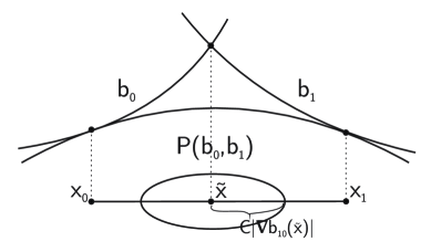
Figure 2: The barriers $b_{0},b_{1}$ and the envelope $P(b_{0},b_{1})$

Suppose now that $\min\{b_{0},b_{1}\}(x_{1})=b_{1}(x_{1})$ (see Figure 2). This case is new compared with the classical setting of Caffarelli [10] and will rely crucially on Proposition 4.5. Since $\min\{b_{0},b_{1}\}(x_{0})=b_{0}(x_{0})$, it follows by continuity of $b_{0}$ and $b_{1}$ that there exists a point $\tilde{x}$ on the straight line segment $\{(1-t)x_{0}+tx_{1}\,:\,t\in[0,1]\}$ connecting $x_{0}$ and $x_{1}$ such that $b_{1}(\tilde{x})=b_{0}(\tilde{x})$, i.e. $\tilde{x}\in b_{10}^{-1}(0)\cap B_{r}(x_{0})$. Hence,

$$\inf_{B_{r}(x_{0})}s_{2}=s_{2}(x_{1})\geq s(x_{1}) =b_{1}(x_{1})-b_{0}(x_{0})-\langle\nabla b_{0}(x_{0}),x_{1}-x_{0}\rangle-Mr^{2}$$

$$=(b_{1}(x_{1})-b_{1}(\tilde{x})-\langle\nabla b_{1}(\tilde{x}),x_{1}-\tilde{x}\rangle)$$

$$\quad+(\langle\nabla b_{1}(\tilde{x}),x_{1}-\tilde{x}\rangle-\langle\nabla b_{0}(\tilde{x}),x_{1}-\tilde{x}\rangle)$$

$$\quad+(\langle\nabla b_{0}(\tilde{x}),x_{1}-\tilde{x}\rangle-\langle\nabla b_{0}(x_{0}),x_{1}-\tilde{x}\rangle)$$

$$\quad+(b_{0}(\tilde{x})-b_{0}(x_{0})-\langle\nabla b_{0}(x_{0}),\tilde{x}-x_{0}\rangle)-Mr^{2}$$

We now estimate from below the last four lines. The first line is minorized by $-2\|b_{1}\|_{C^{2}}|x_{1}-\tilde{x}|^{2}\geq-cr^{2}$, while the third and fourth lines are minorized by $-2\|b_{0}\|_{C^{2}}(|x_{1}-\tilde{x}|^{2}+|x_{0}-\tilde{x}|^{2}+r^{2})\geq-cr^{2}$ (recall (44) and that $|x_{1}-x_{0}|\leq r$, thus $|x_{i}-\tilde{x}|\leq r$), for some $c=c(||b_{0}||_{C^{2}},||b_{1}||_{C^{2}})$. In sum,

$$\inf_{x\in B_{r}(x_{0})}s_{2}\geq(\langle\nabla b_{1}(\tilde{x}),x_{1}-\tilde{x}\rangle-\langle\nabla b_{0}(\tilde{x}),x_{1}-\tilde{x}\rangle)-Cr^{2}\geq-|\nabla b_{10}(\tilde{x})||x_{1}-x_{0}|-Cr^{2}.$$ (50)

Now, by Proposition 4.5, for some $C=C(n)/(1+\|b_{0}\|_{C^{2}}+\|b_{1}\|_{C^{2}})$, there is a ball of radius $C|\nabla b_{10}(\tilde{x})|$ around $\tilde{x}$ that does not intersect $\Lambda$. But $x_{0},x_{1}$ are both in $\Lambda$. Thus,

$$C|\nabla b_{10}(\tilde{x})|\leq|x_{i}-\tilde{x}|,\quad\hbox{for $i=0,1$},$$

hence,

$$2C|\nabla b_{10}(\tilde{x})|\leq|x_{1}-x_{0}|.$$

Plugging this back into (50) yields

$$\inf_{B_{r/2}(x_{0})}s_{2}\geq\inf_{B_{r}(x_{0})}s_{2}\geq-C^{\prime}r^{2},$$ (51)

for $C^{\prime}=C^{\prime}(||b_{0}||_{C^{2}},||b_{1}||_{C^{2}})$. Thus, (46) holds also in this case. This concludes the proof of the Proposition. ∎

Finally, we are in a position to prove the interior $C^{1,1}$ regularity of $b_{\operatorname{env}}$ (10).

Proposition 4.8.

Let $b_{0},b_{1}\in C^{1,1}({B_{1}})$. There exists $C=C(\|b_{0}\|_{C^{2}},\|b_{1}\|_{C^{2}})$ such that

$$\|b_{\operatorname{env}}\|_{C^{2}(B_{1/8})}\leq C.$$

Proof.

First, $b_{\operatorname{env}}$ is differentiable on $B_{1/4}$. This is immediate on $\Lambda^{c}\cap B_{1/4}$ since $b_{\operatorname{env}}$ is harmonic there, while on $\Lambda\cap B_{1/4}$ this follows from Proposition 4.6. Now, $\nabla h$ is Lipschitz continuous on $B_{1/8}$ with Lipschitz constant $C$ if

$$|b_{\operatorname{env}}(x)-b_{\operatorname{env}}(x_{0})-\langle\nabla b_{\operatorname{env}}(x_{0}),x-x_{0}\rangle|\leq C|x-x_{0}|^{2},\quad\forall x_{0},x\in B_{1/8}.$$

This is shown in Proposition 4.6 for $x_{0}\in\Lambda\cap B_{1/8}$, so suppose that $x_{0}\in\Lambda^{c}\cap B_{1/8}$. Denote by $\rho$ the distance of $x_{0}$ to $\Lambda$. If $\rho>1/16$, then we are done since $b_{\operatorname{env}}$ is harmonic on $B_{1/8}(x_{0})$ and so $||b_{\operatorname{env}}||_{C^{2}(B_{1/8}(x_{0}))}\leq C||b_{\operatorname{env}}||_{L^{\infty}(B_{1/4}(x_{0}))}\leq C(\|b_{0}\|_{L^{\infty}(B_{1/4}(x_{0}))},\|b_{1}\|_{L^{\infty}(B_{1/4}(x_{0}))})$ (here we used the fact that (i) $b_{\operatorname{env}}\leq\min\{b_{0},b_{1}\}\leq\min\{\max b_{0},\max b_{1}\}\}$, (ii) since $b_{0},b_{1}$ are bounded from below, the constant function $\min\{\min b_{0},\min b_{1}\}$ is a candidate in the supremum for $b_{\operatorname{env}}$; thus, $b_{\operatorname{env}}\geq\min\{\min b_{0},\min b_{1}\}$, (iii) the $C^{k}$ norm of a harmonic function on a half-ball is estimated by its $C^{0}$ norm on the ball, divided by the radius of the ball to the $k$-th power—this follows from the Poisson representation formula). If $\rho\leq 1/16$ a different argument is needed since the radius of the ball on which $b_{\operatorname{env}}$ is harmonic can be arbitrarily small. Thus, let $x_{1}\in\partial\Lambda\cap B(0,1/4)$ be a point at distance exactly $\rho$ from $x_{0}$. Since $b_{\operatorname{env}}$ is harmonic on $B_{\rho}(x_{0})$ so is $b_{\operatorname{env}}(x)-b_{\operatorname{env}}(x_{1})-\langle\nabla b_{\operatorname{env}}(x_{1}),x-x_{1}\rangle$. Thus, one may express the latter in terms of its boundary values and the Poisson kernel. Since,

$$\nabla^{2}b_{\operatorname{env}}=\nabla^{2}(b_{\operatorname{env}}(x)-b_{\operatorname{env}}(x_{1})-\langle\nabla b_{\operatorname{env}}(x_{1}),x-x_{1}\rangle)$$

then differentiating the aforementioned integral representation twice under the integral sign yields that

$$\|\nabla^{2}b_{\operatorname{env}}(x_{0})\|\leq C\frac{\sup_{x\in B_{\rho}(x_{0})}|b_{\operatorname{env}}(x)-b_{\operatorname{env}}(x_{1})-\langle\nabla b_{\operatorname{env}}(x_{1}),x-x_{1}\rangle|}{\rho^{2}}.$$

Finally, since $B_{\rho}(x_{0})\subset B_{2\rho}(x_{1})$ it follows from Proposition 4.6 that the right hand side is majorized by

$$C\frac{\sup_{x\in B(x_{1},2\rho)}|b_{\operatorname{env}}(x)-b_{\operatorname{env}}(x_{1})-\langle\nabla b_{\operatorname{env}}(x_{1}),x-x_{1}\rangle|}{\rho^{2}}\leq C,$$

as desired. ∎

Purdue University

tdarvas@math.purdue.edu

University of Maryland

yanir@umd.edu

References

- [1] E. Bedford, B.A. Taylor, The Dirichlet problem for a complex Monge–Ampère equation, Invent. Math. 37 (1976), 1–44.
- [2] J. Benoist, J.-B. Hiriart-Urruty, What is the subdifferential of the closed convex hull of a function?, SIAM J. Math. Anal. 27 (1996), 1661–1679.
- [3] R. Berman, Bergman kernels and equilibrium measures for line bundles over projective manifolds, Amer. J. Math. 131 (2009), 1485–1524.
- [4] R.J. Berman, regularity of weak geodesic segments in the space of metrics on a line bundle, preprint, May 2014.
- [5] R. Berman, From Monge–Ampère equations to envelopes and geodesic rays in the zero temperature limit, preprint, arxiv:1307.3008.
- [6] R. Berman, J. P. Demailly, Regularity of plurisubharmonic upper envelopes in big cohomology classes, in: Perspectives in analysis, geometry and topology, Progr. Math. 296, Birkhäuser/Springer, 2012, 39–66.
- [7] B. Berndtsson, A Brunn–Minkowski type inequality for Fano manifolds and the Bando–Mabuchi uniqueness theorem, preprint, arxiv:1103.0923.
- [8] Z. Blocki, A gradient estimate in the Calabi-Yau theorem, Math. Ann. 344 (2009), 317-327.
- [9] H.-J. Bremermann, On a generalized Dirichlet problem for plurisubharmonic functions and pseudo-convex domains. Characterization of Silov boundaries, Trans. Amer. Math. Soc. 91 (1959) 246–276.
- [10] L.A. Caffarelli, The obstacle problem, Accademia Nazionale dei Lincei, Scuola Normale Superiore, 1998.
- [11] L.A. Caffarelli, S. Salsa, A geometric approach to free boundary problems, Amer. Math. Soc., 2005.
- [12] T. Darvas, Envelopes and Geodesics in Spaces of Kähler Potentials, arXiv:1401.7318.
-
[13]
J. P. Demailly, Complex Analytic and Differential Geometry,
http://www-fourier.ujf-grenoble.fr/~demailly/manuscripts/agbook.pdf - [14] S.K. Donaldson, Symmetric spaces, Kähler geometry and Hamiltonian dynamics, in: Northern California Symplectic Geometry Seminar (Ya. Eliashberg et al., Eds.), Amer. Math. Soc., 1999, pp. 13–33.
- [15] W. Fenchel, On conjugate convex functions, Canad. J. Math. 1 (1949), 73–77.
- [16] A. Griewank, P.J. Rabier, On the smoothness of convex envelopes, Trans. Amer. Math. Soc. 322 (1990), 691–709.
- [17] V. Guedj (Ed.), Complex Monge-Ampère equations and geodesics in the space of Kähler metrics. Lecture Notes in Math. 2038, 2012.
- [18] W. He, On the space of Kähler potentials, preprint, arxiv:1208.1021.
- [19] J.-B. Hiriart-Urruty, C. Lemaréchal, Convex analysis and minimization algorithms II, Springer, 1993.
- [20] T. Jeffres, R. Mazzeo, Y.A. Rubinstein, Kähler–Einstein metrics with edge singularities, (with an appendix by C. Li and Y.A. Rubinstein), preprint, arxiv:1105.5216.
- [21] B. Kirchheim, J. Kristensen, Differentiability of convex envelopes, C. R. Acad. Sci. Paris, Ser. I 333 (2001), 725–728.
- [22] S. Kolodziej, The complex Monge-Ampère equation and pluripotential theory, Mem. Amer. Math. Soc. 178 (2005), no. 840.
- [23] C.O. Kiselman, The partial Legendre transformation for plurisubharmonic functions, Invent. Math. 49 (1978), 137–148.
- [24] , Plurisubharmonic functions and their singularities, in: Complex potential theory (P.M. Gauthier et al., Eds.), Kluwer, 1994, pp. 273–323.
- [25] T. Mabuchi, Some symplectic geometry on compact Kähler manifolds I, Osaka J. Math. 24, 1987, 227–252.
- [26] S. Mandelbrojt, Sur les fonctiones convexes, C. R. Acad. Sci. Paris 209 (1939), 977–978.
- [27] A. Petrosyan, T. To, Optimal regularity in rooftop-like obstacle problem, Comm. Partial Differential Equations 35 (2010), 1292–1325.
- [28] A. Petrosyan, H. Shahgholian, N. Uraltseva, Regularity of free boundaries in obstacle-type problems, Amer. Math. Soc., 2012.
- [29] R.T. Rockafellar, Convex analysis, Princeton University Press, 1970.
- [30] J. Ross, D. Witt Nystrom, Analytic test configurations and geodesic rays, J. Symplectic Geom. 12 (2014), 125–169.
- [31] , Envelopes of positive metrics with prescribed singularities, arXiv:1210.2220.
- [32] Y.A. Rubinstein, Some discretizations of geometric evolution equations and the Ricci iteration on the space of Kähler metrics, Adv. Math. 218 (2008), 1526–1565.
- [33] , Smooth and singular Kähler–Einstein metrics, preprint, arxiv:1404.7451.
- [34] Y.A. Rubinstein, S. Zelditch, The Cauchy problem for the homogeneous Monge–Ampère equation, II. Legendre transform, Adv. Math. 228 (2011), 2989–3025.
- [35] , The Cauchy problem for the homogeneous Monge–Ampère equation, III. Lifespan, preprint, arxiv:1205.4793.
- [36] S. Semmes, Interpolation of spaces, differential geometry and differential equations, Rev. Mat. Iberoamericana 4 (1988), 155–176.
- [37] , Complex Monge-Ampère and symplectic manifolds, Amer. J. Math. 114 (1992), 495–550.
- [38] D. Wu, Kähler-Einstein metrics of negative Ricci curvature on general quasi-projective manifolds, Comm. Anal. Geom. 16 (2008), 395–435.