Validating the 2PI resummation: the Bloch-Nordsieck example

Abstract

In this work we provide a numerical method to obtain the Bloch-Nordsieck spectral function at finite temperature in the framework of the 2PI approximation. We find that the 2PI results nicely agree with the exact one, provided we perform a coupling constant matching. In the paper we present the resulting finite temperature running of the 2PI coupling constant. This result may apply for the finite temperature behavior of the coupling constant in QED, too.

I Introduction

The infrared limit of the QED was modeled by Bloch and Nordsieck in 1937, and their treatment of the IR singularities has become a textbook material since. In the framework of the Bloch-Nordsieck (B-N) model one is able to resum all of the radiative contributions to the fermionic Green’s function generated by ultra-soft photons. A detailed discussion of this calculation can be found in the original paper of Bloch and Nordsieck BN , in textbooks BogoljubovShirkov ,Fried and in Jakovac:2011aa .

Besides an exact solution one can also give solutions in different approximations. In particular the 2-particle-irreducible (2PI) approximation 2PIhist is a well known tool to study the quasiparticle properties of the system. One of the biggest challenge in front of the 2PI techniques is the representations of symmetries, in particular gauge symmetries RS1 . The study of B-N model provides an excellent tool to test the reliability of fixed gauge calculations.

In our paper Jakovac:2011aa we used the 2PI functional method to study the B-N model at zero temperature. The spectrum could be obtained by applying numerical calculations. We found on the one hand the disappointing fact that the fit comparison to the exact propagator was not very promising (see Jakovac:2011aa ), on the other hand, unlike in the old-fashioned perturbation theory, the spectrum remained regular even in the highly infrared regime (no infrared singularity observed at the mass shell).

At finite temperature there are several studies in the literature IancuBlaizot1 ; IancuBlaizot2 ; Fried:2008tb to derive the behavior of the fermion propagator. In our paper Jakovac:2011aa we developed a method to reproduce the exact result using the Ward-Takahashi identities at zero temperature (cf. also Alekseev:1982dk ). This could have been generalized to finite temperature in Jakovac:2013aa . With the help of this method we managed to obtain a fully analytical form of the excitation spectrum. Having these analytic results gives us a perfect opportunity to investigate the validity of the 2PI quasiparticle description of an interacting quantum field theory at finite temperature.

The purpose of the present paper is to show how the 2PI works at finite temperature. We will derive the spectral function numerically and compare it to the exactly calculated case. The upshot is: there exists a mapping between the coupling constants of the 2PI and the exact results in such a way that the two spectral function overlap almost entirely. This is a highly nontrivial result, since the exact spectral function is an asymmetric function of the frequency, rather different from a simple Lorentzian. The most important message to the 2PI community is that our result validates the 2PI approximation method at non-zero temperature, and only a finite reparametrization of the theory is needed.

From the perturbative point of view the 2PI technique resums the two particle irreducible diagrams, but the coupling constant and also the higher point functions are remained unchanged. So for a certain 2PI diagram there exists another infinite set of diagrams providing coupling constant modification. In the sense of the renormalization group we may try to take into account the sum of these diagrams effectively as a temperature dependent (running) coupling constant. Since we now know the value of an observable exactly (the electron spectral function for any frequency and temperature in a given gauge), the best method to extract the temperature dependent coupling is to compare the 2PI and the exact results. This is done in the present paper.

The structure of the paper is as follows. First we give an introduction to the Bloch-Nordsieck model itself and to the conventions of the finite temperature real time formalism. In Section III we recap the zero temperature results: the one-loop correction obtained from perturbation theory (PT) and the implementation of the 2PI numerics. In Section IV we derive the one-loop self energy at $T\neq 0$ and show its consistency with the zero temperature result by taking the $T\rightarrow 0$ limit. Then we calculate the expression for the discontinuity of the self energy for the 2PI procedure. The numerical implementation of the calculation happens in a similar fashion as the zero temperature one. In Section V we present our results obtained from the numerics and the comparison to the exact result Jakovac:2013aa . We found a non-trivial mapping of the coupling between the two calculation methods from which we conclude: the 2PI, although it is an approximation, at finite temperature it gives a perfect qualitative description of the collective excitation of the system.

II The properties of the Bloch-Nordsieck model

The Bloch-Nordsieck model was designed to describe accurately the low energy regime of quantum electrodynamics. Considering the contributions to the fermion self energy only from the deep infrared photons, reducing the Dirac spinor to a one component fermion is well justified. Indeed, at this energy scale photons do not have enough energy even to flip the spin of the fermion, not to mention the pair creation BN . In this respect, one can substitute a four vector $u_{\mu}$ in the place of the $\gamma_{\mu}$ matrices which is considered as the four velocity of the fermion.

The Lagrangian then reads:

$$\mathcal{L}=-\frac{1}{4}F_{\mu\nu}F^{\mu\nu}+\Psi^{\dagger}(iu_{\mu}D^{\mu}-m)\Psi.$$ (1)

Where the usual notations for the field-strength tensor and for the covariant derivative are used: $F_{\mu\nu}=\partial_{\mu}A_{\nu}-\partial_{\nu}A_{\mu}$ and $D_{\mu}=i\partial_{\mu}-eA_{\mu}$, respectively. Here, as it was mentioned above, $u_{\mu}$ is a four velocity, but we can also choose the form $u=(1,\bf{v})$, with ${\bf{v}}={\bf{u}}/u_{0}$ by rescaling the fermionic field as $\Psi\rightarrow\Psi/\sqrt{u_{0}}$ and the fermion mass by $m\rightarrow mu_{0}$.

It is possible to obtain exactly the full fermion propagator associated with this theory both for zero and finite temperatures as it is presented in Jakovac:2011aa and Jakovac:2013aa , respectively. Now we are going to discuss the notations and conventions that we are using in this paper.
For the calculations we used the real time formalism (details in Jakovac:2013aa ,LeBellac ). The propagators are matrices in this convention:

$$i{\cal G}_{ab}(x)=\left\langle{T_{C}\Psi_{a}(x)\Psi_{b}^{\dagger}(0)}\right\rangle\qquad\mathrm{and}\qquad iG_{\mu\nu,ab}(x)=\left\langle{T_{C}A_{\mu a}(x)A_{\nu b}(0)}\right\rangle,$$ (2)

where $T_{C}$ denotes ordering with respect to the contour variable (contour time ordering). At finite temperature with help of the KMS relation we can determine $G_{12}$ and $G_{21}$

$$iG_{12}(k)=\pm n_{\pm}(k_{0})\varrho(k),\qquad iG_{21}(k)=(1\pm n_{\pm})(k_{0})\varrho(k),$$ (3)

where

$$n_{\pm}(k_{0})=\frac{1}{e^{\beta k_{0}}\mp 1}\quad\mathrm{and}\quad\varrho(k)=iG_{21}(k)-iG_{12}(k)$$ (4)

are the distribution functions (Bose-Einstein (+) and Fermi-Dirac (-) statistics), and the spectral function, respectively. We will also use R/A formalism Jakovac:2013aa , where

$$G_{rr}=\frac{G_{21}+G_{12}}{2},\quad G_{ra}=G_{11}-G_{12},\quad\varrho=iG_{ra}-iG_{ar}.$$ (5)

The $G_{ra}$ propagator is the retarded, the $G_{ar}$ is the advanced propagator, $G_{rr}$ is usually called the Keldysh propagator.

At zero temperature the (free) fermionic Feynman-propagator reads:

$${\cal G}_{0}(p)=\frac{1}{u_{\mu}p^{\mu}-m+i\varepsilon}.$$ (6)

It has a single pole which means that there are no antiparticles in the model. Consequently, closed fermion loops are excluded, thus there is no self energy correction to the photon propagator at zero temperature. Physically this means that the energy is not sufficient to excite the antiparticles. We interpret $u^{\mu}$ as the fermionic four-velocity, and since it is fixed, the soft photons cannot change it (no fermion recoil). In fact this means that the fermion is a hard probe of the system, hence not part of the thermal medium IancuBlaizot1 ; IancuBlaizot2 . This is also supported by the spin-statistics theorem PeshkinSchroeder which would forbid a one-component fermion field. Consequently we will neglect the ’12’ fermion propagator, too: ${\cal G}_{12}=0$.

The exact photon propagator reads in Feynman gauge

$$G_{ab,\mu\nu}(k)=-g_{\mu\nu}G_{ab}(k),\qquad G_{ra}=\frac{1}{k^{2}}\biggr{|}_{k_{0}\to k_{0}+i\varepsilon},\quad\varrho(k)=2\pi\mathop{\textrm{sgn}}(k_{0})\delta(k^{2}),$$ (7)

all other propagators can be expressed using identities (3) and (5).

III Recap of T=0 2PI calculations

The main idea is to use the exact propagators in the perturbation theory as building blocks of a loop integral, where the exact propagator is determined self-consistently using skeleton diagrams as resummation patterns. The one-loop 2PI fermion self energy diagram in the case of the Bloch-Nordsieck model generates the resummation of all the “rainbow” diagrams. One needs to take care of the UV divergences, too, on which we perform a renormalization with the same form of divergent parts of the counterterms as in the 1-loop case.

At zero temperature we have the following self-consistent system of equations in the 2PI approximation

$${\cal G}(p) = \frac{1}{{\cal G}_{0}^{-1}(p)-\Sigma(p)},$$ (8)

$$-i\Sigma(p) = (-ie)^{2}{\int\!\frac{d^{4}k}{(2\pi)^{4}}\,}iG_{\mu\nu}(k)i{\cal G}(p-k).$$ (9)

Here ${\cal G}_{0}$ and ${\cal G}$ stand for the free and the dressed fermion propagator. $G_{\mu\nu}$ is the photon propagator.

III.1 The one-loop correction

In strict perturbation theory (PT) we use the propagators from Eq.(6) and (7) to compute the self energy. We choose a reference frame which in $u^{\mu}=(1,0,0,0)$, and we find using dimensional regularization

$$\Sigma_{1loop}(p_{0})=\frac{\alpha}{\pi}(p_{0}-m)\left(-\ln{\frac{m-p_{0}}{\mu}}+{\cal D}_{\epsilon}\right).$$ (10)

Here $\mu$ is the renormalization scale. The divergent part ${\cal D}_{\epsilon}$ has the following expression:

$${\cal D}_{\epsilon}=\frac{1}{2\epsilon}+\frac{1}{2}\left(\ln{4\pi}-\gamma_{E}\right).$$ (11)

We renormalized the self energy using the $\overline{\text{MS}}$ scheme, by which the counterterms read as

$$\delta Z_{1,\overline{\text{MS}}}=\delta_{m,\overline{\text{MS}}}=\frac{\alpha}{\pi}D_{\epsilon},$$ (12)

where $\delta Z_{1,\overline{\text{MS}}}$, $\delta_{m,\overline{\text{MS}}}$ are the wave function renormalization and the multiplicative mass renormalization, respectively. Hence, the renormalized self energy is

$$\Sigma_{1loop}^{ren}=-\frac{\alpha}{\pi}(p_{0}-m)\ln{\frac{m-p_{0}}{\mu}}.$$ (13)

For the details see Jakovac:2011aa .

III.2 The 2PI procedure at $T=0$

In the 2PI approach we treat Eq.(8) and Eq.(9) self-consistently. Then we implement the following steps numerically Jakovac:2011aa , which will be applied at finite T, too:
step 1: We calculate the discontinuity of the self-energy in order to use it the spectral representation of the retarded Green’s function.

$$\Sigma(p)=ie^{2}{\int\!\frac{d^{4}k}{(2\pi)^{4}}\,}G_{\mu\nu}{\cal G}(p-k) = ie^{2}\int\limits_{0}^{\infty}\frac{d\omega}{2\pi}{\int\!\frac{d^{4}k}{(2\pi)^{4}}\,}\frac{1}{k^{2}+i\epsilon}\frac{\rho(\omega)}{p_{0}-k_{0}-\omega+i\epsilon}$$ (14)

$$\Sigma(p) = \int\limits_{0}^{\infty}\frac{d\omega}{2\pi}\rho(\omega)\Sigma_{1-loop}(p,\omega)$$ (15)

Now we can take the discontinuity

$$\mathop{\textrm{Disc}}\limits_{p_{0}}\Sigma(p)=\int\limits_{0}^{\infty}\frac{d\omega}{2\pi}\rho(\omega)\mathop{\textrm{Disc}}\limits_{p_{0}}\Sigma_{1-loop}(p,\omega)=\frac{\alpha}{\pi}\int\limits_{0}^{\infty}d\omega(p_{0}-\omega)\rho(\omega).$$ (16)

In both equations we introduced the fermion spectral function $\rho(p)$. In our algorithm it serves as an input, which is usually the free fermion spectral function $\rho(p)=2\pi\delta(p-m)$.
step 2: Here we calculate the real part of self energy from its discontinuity. For this purpose we use the Kramers-Kronig relation:

$$\text{Re}\Sigma(p_{0},{\bf{{\bf p}}})=\int\limits_{-\infty}^{\infty}\frac{d\omega}{2\pi}\frac{\mathop{\textrm{Disc}}_{\omega}i\Sigma(\omega,{\bf p})}{p_{0}-\omega+i\epsilon}.$$ (17)

step 3: We renormalize the real part of the self energy using the ”on-mass-shell” (OMS) renormalization scheme:

$$\text{Re}\Sigma(p_{0}=m) =0,$$ (18)

$$\displaystyle\left.\frac{d\text{Re}\Sigma(p_{0})}{dp_{0}}\right|_{p_{0}=m} =0.$$ (19)

step 4: From all of this information we construct the new spectral function, which reads as

$$\rho(p)=\frac{2\text{Im}\Sigma(p)}{(p_{0}-m-\text{Re}\Sigma(p))^{2}+(\text{Im}\Sigma(p))^{2}}.$$ (21)

step 5: We set the new spectral function to be our new input, and iterate this procedure till it converges.
step 4+: As an additional step we had to include a rescaling of the spectral function which was necessary to stabilize the convergence. This step is not needed at non-zero temperature.
For the zero temperature case we obtained the dressed propagator for the fermion. From the analysis it turned out that this result, being an approximation, is far from the exact solution although it is infrared finite, which cannot be claimed about the PT calculation (see Jakovac:2011aa ).

IV Non-zero temperature

We are working in the real time formalism, hence the Green’s functions in this picture are going to have a matrix structure. We choose the $R/A$ basis for the matrix representation to calculate the retarded self energy. First we are going to consider the one-loop correction then we present a derivation of the 2PI resummed spectral function at finite temperature. To evaluate its self-consistent equations we will use a numerical approach which is similar to what we discussed above for the $T=0$ case. The integral equation for the retarded self energy at non-zero temperature in Feynman gauge reads as:

$$\Sigma_{ar}(p)=ie^{2}{\int\!\frac{d^{4}k}{(2\pi)^{4}}\,}\left[G_{rr}(k){\cal G}_{ra}(p-k)+G_{ra}(k){\cal G}_{rr}(p-k)\right].$$ (22)

Where $G$ and ${\cal G}$ stands for the propagator of the photon and the fermion, respectively. On Fig.(1) we can see the pictorial representation of the fermion self energy using Feynman diagrams.

Figure 1: The diagrammatic representation of the self energy. The wavy line corresponds to the free (here also the exact) photon propagator with a loop momentum $k$ and the double solid line is for the exact fermion propagator with momentum $p-k$. Both the polarization and the Keldysh indices are shown.

Now, if we take the discontinuity we will have:

$$\mathop{\textrm{Disc}}\limits_{p_{0}}\Sigma_{ar}(p)=e^{2}{\int\!\frac{d^{4}k}{(2\pi)^{4}}\,}\left[G_{rr}(k)\rho_{f}(p-k)+\rho_{\gamma}(k){\cal G}_{rr}(p-k)\right].$$ (23)

Here $\rho_{f}$ and $\rho_{\gamma}$ are the spectral functions to the fermion and the photon, respectively. In general we can express the $rr$ propagators by the spectral function combining with the distribution function of the corresponding spin statistics:

$${\cal G}_{rr}(p) = \left(\frac{1}{2}-n_{f}(p_{0})\right)\rho_{f}(p),$$ (24)

$$G_{rr}(p) = \left(\frac{1}{2}+n_{b}(p_{0})\right)\rho_{\gamma}(p).$$ (25)

When inserting these expressions into Eq.(23), we get

$$\mathop{\textrm{Disc}}\limits_{p_{0}}\Sigma_{ar}(p) = e^{2}{\int\!\frac{d^{4}k}{(2\pi)^{4}}\,}\left[\left(\frac{1}{2}+n_{b}(k_{0})\right)\rho_{\gamma}(k)\rho_{f}(p-k)+\rho_{\gamma}(k)\left(\frac{1}{2}-n_{f}(p_{0}-k_{0})\right)\rho_{f}(p-k)\right]=$$ (26)

$$= e^{2}{\int\!\frac{d^{4}k}{(2\pi)^{4}}\,}\left(1+n_{b}(k_{0})-n_{f}(p_{0}-k_{0})\right)\rho_{\gamma}(k)\rho_{f}(p-k).$$

In the last step of Eq.(26) we get the most general form of the equation, as long as we do not specify the corresponding spectral functions.

IV.1 One-loop correction at $T\neq 0$

For the one-loop case we have to plug in the spectral function of the free theory both for the fermion and gauge fields. By performing this substitution our equation reads as

$$\mathop{\textrm{Disc}}\limits_{p_{0}}\Sigma_{ar}(p) = e^{2}{\int\!\frac{d^{4}k}{(2\pi)^{4}}\,}\left(1+n_{b}(k_{0})-n_{f}(p_{0}-k_{0})\right)2\pi\mathop{\textrm{sgn}}{k_{0}}\delta(k_{0}^{2}-{\bf k}^{2})2\pi\delta\left(u_{0}(p_{0}-k_{0})-{\bf u}({\bf p}-{\bf k})-m\right)=$$ (27)

$$= \frac{e^{2}}{8\pi^{3}}\int\limits_{0}^{\infty}\!dk{\bf k}^{2}\int\limits_{-1}^{1}\!dx\frac{(2\pi)^{2}}{2|{\bf k}|}\left[\left(1+n_{b}(|{\bf k}|)-n_{f}(p_{0}-|{\bf k}|)\right)\delta\left(u_{0}p_{0}-{\bf u}{\bf p}-u_{0}|{\bf k}|-|{\bf u}||{\bf k}|x-m\right)+\right.$$

$$+ \left.\left(n_{b}(|{\bf k}|)+n_{f}(p_{0}+|{\bf k}|)\right)\delta\left(u_{0}p_{0}-{\bf u}{\bf p}+u_{0}|{\bf k}|-|{\bf u}||{\bf k}|x-m\right)\right].$$

Here we introduced the variable $x$ which stands for the cosine of the angle between the two spatial three-vectors ${\bf u}$ and ${\bf k}$. For the sake of simplicity in the following we are going to use the notations $pu\equiv p_{0}u_{0}-{\bf{pu}}$ for the Minkowski product, and $k\equiv|{\bf k}|,u\equiv|{\bf u}|$ for the absolute values of the three vectors ${\bf k}$ and ${\bf u}$, respectively.
First we perform the angular integration for $x$:

$$\mathop{\textrm{Disc}}\limits_{p_{0}}\Sigma_{ar}(p)=\frac{e^{2}}{4\pi u}\left(\Theta(pu-m)\int\limits_{\frac{pu-m}{u+u_{0}}}^{\frac{pu-m}{u-u_{0}}}\!dk\left(1+n_{b}(k)-n_{f}(p_{0}-k)\right)+\Theta(m-pu)\int\limits_{\frac{m-pu}{u+u_{0}}}^{\frac{m-pu}{u-u_{0}}}\!dk\left(n_{b}(k)+n_{f}(p_{0}+k)\right)\right)$$ (28)

Now we are going to use the fact that the fermion in this system is a hard probe, thus it is not part of the heat-bath IancuBlaizot1 ; IancuBlaizot2 . This manifests already in Eq.(26) in a way that we need to set the Fermi-Dirac distribution to zero, otherwise we would face with inconsistencies when one would try to take the $T\rightarrow 0$ limit:

$$n_{f}\equiv 0\text{ (in the B-N framework).}$$ (29)

In that case Eq.(28) simplifies in the following way:

$$\mathop{\textrm{Disc}}\limits_{p_{0}}\Sigma_{ar}(p)=\frac{e^{2}}{4\pi u}\int\limits_{\frac{pu-m}{u+u_{0}}}^{\frac{pu-m}{u-u_{0}}}\!dk\left(1+n_{b}(k)\right).$$ (30)

Evaluating the integral one gets a result consistent with the $T=0$ case:

$$\mathop{\textrm{Disc}}\limits_{p_{0}}\Sigma_{ar}(p)=\frac{e^{2}}{2\pi}\Theta(pu-m)(pu-m)+\frac{Te^{2}}{4\pi u}\ln\left(\frac{1-e^{-\beta\frac{pu-m}{u-u_{0}}}}{1-e^{-\beta\frac{pu-m}{u+u_{0}}}}\right).$$ (31)

This gives us the desired result for the $T\rightarrow 0$ limit, namely $\mathop{\textrm{Disc}}\limits_{p_{0}}\Sigma_{ar}(p)=\frac{e^{2}}{2\pi}\Theta(pu-m)(pu-m)$.

IV.2 Non-zero temperature calculations for the 2PI scheme

Now we are going to derive the 2PI resummed result for the finite temperature theory. Let us consider Eq.(8) and Eq.(22). Instead of calculating the one-loop correction by inserting free propagators, we are going to use the self-consistent fermion propagator so defining a self-consistent system of integral equations. We stick to the physical picture that the fermion is not part of the thermal medium, Eq.(29) . Using the calculation in Eq.(27) we arrive to an expression for the discontinuity of the self energy for general fermion propagator:

$$\mathop{\textrm{Disc}}\limits_{p_{0}}\Sigma_{ar}(p) = e^{2}{\int\!\frac{d^{4}k}{(2\pi)^{4}}\,}\left(1+n_{b}(k_{0})\right)\rho_{\gamma}(k)\rho_{f}(p-k)$$ (32)

$$= e^{2}{\int\!\frac{d^{4}k}{(2\pi)^{4}}\,}\left(1+n_{b}(k_{0})\right)\frac{2\pi}{2k}(\delta(k_{0}-k)-\delta(k_{0}+k))\bar{\rho}_{f}(up-uk-m).$$

Here we used the free photon propagator as above and for the general spectral function of the fermion we introduced the notation $\rho_{f}(p)=\bar{\rho}_{f}(up-m)$. After some algebra we find

$$\mathop{\textrm{Disc}}\limits_{p_{0}}\Sigma_{ar}(p)=\frac{e^{2}}{8\pi^{2}}\int\limits_{-\infty}^{\infty}\!dk\int\limits_{-1}^{1}\!dxkn_{b}(k)\bar{\rho}_{f}(w+(u_{0}+ux)k).$$ (33)

Here we defined $w:=up-m$, and $x$ represents the angle between the spatial parts of $k^{\mu}$ and $u^{\mu}$, so $xku$ is the scalar product of two three-dimensional vectors like in the one-loop calculation. Actually, this can be written in a more elegant, and for the numerical implementation, a more useful way. We introduce the variable $z$ as the argument of the function $\bar{\rho}_{f}$:

$$\mathop{\textrm{Disc}}\limits_{p_{0}}\Sigma_{ar}(p) = \frac{e^{2}}{8\pi^{2}}\frac{1}{u}\int\limits_{-\infty}^{\infty}\!dk\int\limits_{w+(u_{0}-u)k}^{w+(u_{0}+u)k}\!dz\bar{\rho}_{f}(z)n_{b}(k)=\frac{e^{2}}{8\pi^{2}}\frac{1}{u}\int\limits_{-\infty}^{\infty}\!dz\bar{\rho}_{f}(z)\int\limits_{\frac{z-w}{u_{0}-u}}^{\frac{z-w}{u_{0}+u}}\!dkn_{b}(k).$$ (34)

In the case when the length of the three-velocity tends to zero,$u\rightarrow 0$ , we have

$$\mathop{\textrm{Disc}}\limits_{p_{0}}\Sigma_{ar}(p_{0})=\frac{\alpha}{\pi}\int\limits_{-\infty}^{\infty}dz\bar{\rho}_{f}(z)(p_{0}-m-z)(1+n_{b}(p_{0}-m-z)).$$ (35)

For $u\neq 0$

$$\mathop{\textrm{Disc}}\limits_{p0}\Sigma_{ar}(w)=\frac{\alpha}{2\pi}\int\limits_{-\infty}^{\infty}dz\bar{\rho}_{f}(z)\frac{T}{u}\ln\frac{1-e^{-\beta\frac{z-w}{u_{0}-u}}}{1-e^{-\beta\frac{z-w}{u_{0}+u}}}.$$ (36)

We set $m=0$, this can be done without the loss of generality since the two expressions in Eq.(35) and Eq.(36) depends on the variable $w=up-m$ only. That means the theory is not sensitive where the mass-shell is placed, it can be anywhere on the real line. With these formulae we can find the solution of the self-consistent system of equations numerically, in a similar way we did it in the case of zero temperature (step 1 - step 5), but this time we insert the finite temperature ingredients (Eqs. 35 and 36).

V 2PI results

We are implementing the same numerical method that we used for the zero temperature case (Section III/B); the renormalization procedure goes in the same way. First we observe that a small thermal mass is generated. Interestingly this thermal mass is negative, it shifts the spectral function to the left. In the exact solution in Jakovac:2013aa we found a zero thermal mass, thus we can consider it as an artifact of the 2PI approximation, which can be incorporated into the mass, or into the notation $w=up-m$. We should also remark that the B-N theory describes only the softest photons while in a realistic theory the mass modification dominantly is due to the modes with higher momenta.

V.1 The zero velocity case

By applying the algorithm described in Section III/B we can obtain the spectral function derived from the 2PI approximation for the theory, using Eq.(35) as the self energy input. On Fig. 2 we can see the spectral function for different coupling values and for different temperatures. The spectrum exhibits a pole, its width is growing with increasing coupling constant and with increasing temperature.

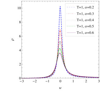
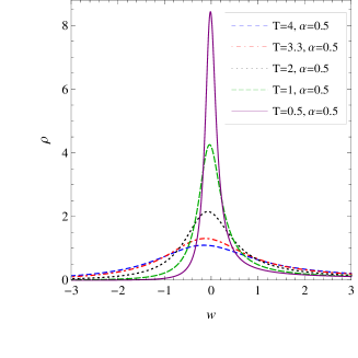
a.)                                                            b.)

Figure 2: The coupling constant dependence of the spectral function in the 2PI approximation (a.) at fixed temperature $T=1$, and (b.) at fixed fixed coupling value, $\alpha=0.5$. The curves widen with growing coupling, and growing temperature.

In the Dyson-Schwinger approach the exact spectral function can be derived in a closed form (at least in the the zero velocity case). We wish to compare the 2PI results to our analytical expression obtained in Jakovac:2013aa :

$$\rho(w)=\frac{N_{\alpha}\beta\sin{(\alpha)}e^{\beta w/2}}{\cosh(\beta w)-\cos(\alpha)}\frac{1}{\left|\Gamma\left(1+\frac{\alpha}{2\pi}+i\frac{\beta w}{2\pi}\right)\right|^{2}}.$$ (37)

Here we used the notation $w=p_{0}-m$ again and $N_{\alpha}$ is a normalization factor. Both for the 2PI approximation and the D-S calculation we assumed a normalization prescription, which assigned by $\int_{w}\rho=1$ sum rule.

To check the quality of the 2PI approximation, we can compare the resulting spectral function with the exact one. The comparison can be seen on Fig.(3).

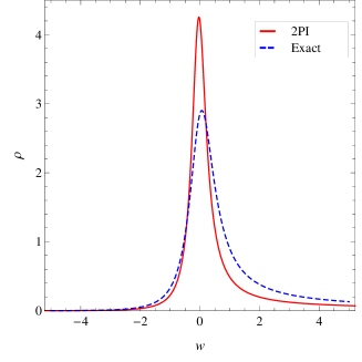
Figure 3: Comparing the 2PI resummed spectral function to the exact one. The solid red line is obtained from the 2PI resummation while the dashed blue is the exact spectral function. Both of them are at T=1 and the couplings are $\alpha_{ex}=\alpha_{2PI}=0.5$.

We can see immediately that the two spectra are not very similar. The reason is, as we discussed in the Introduction, that the 2PI approximation do not sum up all the diagrams, in particular the coupling constant corrections. To improve the 2PI calculation, therefore, we can try to take into account the resummation of these diagrams effectively in a renormalization group inspired way, as a temperature dependent coupling constant. We should use a nonperturbative matching procedure, and choose that value of $\alpha_{2PI}$ which reproduces the exact result the most accurately. For a perfect matching not only the coupling constant, but also the higher point functions should also be resummed. But we may hope that the most important effect comes from the relevant couplings, in this case from $\alpha_{2PI}$.

Therefore our strategy will be to find the best, temperature dependent value of the coupling constant $\alpha_{2PI}$ which yields the best match between the exact and the 2PI spectral functions. As we can see on Fig. 4, there exist such a value, where the matching is almost perfect. We can observe that the fit is excellent not just at the close vicinity of the peak region, but also for much larger momentum regime, and it can give an account also for the asymmetric form of the exact spectral function. For asymptotically large momenta we expect that the two curves do not agree, according to Jakovac:2011aa , this can also be observed on Fig. 4. This result is a strong argument in favor of the usability of 2PI technique at finite temperature also for gauge theories.

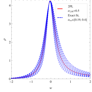
(a)

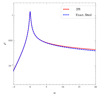
(b)

Figure 4: The fitting of the exact spectral function on the 2PI spectrum in linear (a.) and logarithmic (b.) plot. We can see an exact match at the peak and a small deviation in the asymptotics. The fit yields $\alpha_{2PI}=0.5$ for $\alpha_{ex}=0.293$ at $T=1$.

Hence we can say that the coupling which takes the value of $\alpha_{2PI}=0.5$ in the 2PI resummation at $T=1$ is equivalent to an $\alpha_{ex}=0.293$ in the D-S calculation at the same temperature. One can also conclude that the vertex corrections (which are absent in the 2PI self-energy calculations) have a role to modify the value of the renormalized coupling. In the following we are going to look for a general relation between $\alpha_{2PI}$ and $\alpha_{ex}$.

We can repeat the strategy above for different temperatures. In this way we can determine a relation $\alpha_{2PI}(\alpha_{ex},T)$ (technically it is simpler to obtain $\alpha_{ex}(\alpha_{2PI},T)$ and invert this relation). This provides the finite temperature dependence, or finite temperature “running” of the 2PI coupling constant.

We expect that for small couplings the exact and the perturbative values agree, since the perturbation theory gives $\alpha_{ex}=\alpha_{2PI}+{\cal O}(\alpha_{2PI}^{2})$. This is indeed the case. For larger couplings, however, the linear relation changes. Interestingly, we can observe that two different type of functions describe the relation between the couplings depending on the temperature. The first type of function which gives the mapping between the to couplings is valid in the interval $T\in[0,12.03]$. This relation can be obtained by a one-parameter fit between the 2PI and the exact couplings, namely:

$$\alpha_{2PI}=A_{T}(e^{\frac{\alpha_{ex}}{A_{T}}}-1).$$ (38)

The result is shown on Fig. 5/a., the fit parameters ($A_{T}$) are listed in Tables 1 and 2. From this relation we immediately see that for small $\alpha_{2PI}$ the relation of the couplings is linear

$$\alpha_{2PI}\approx\alpha_{ex}+\mathcal{O}\left(\frac{\alpha_{ex}^{2}}{A_{T}}\right).$$ (39)

This tells us that the 2PI and the exact couplings are the same for the perturbative region, meaning that we can rely on the results obtained by 2PI calculations in this regime. Thus if we are using couplings which are in the order of the fine structure constant of QED ($\alpha=1/137$) for instance, one does not even have to worry about the temperature dependence of Eq.(38).

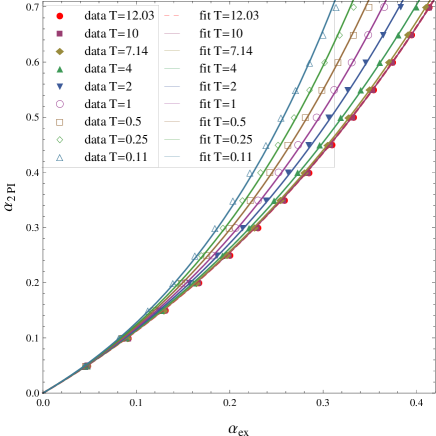
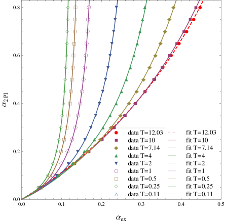
          a.)                                                                             b.)

Figure 5: The relation between the 2PI and the exact coupling at $u=0$ for temperatures a.) $T\in[0,12.03]$ and b.) $T\in(12.03,\infty)$, respectively. The dashed red line indicates the limiting function at $T=12.03$, for details see the text.

$T$	$0.11$	$0.25$	$0.5$	$1$	$2$	$4$	$7.14$	$10$	$12.03$
$A_{T}$	$0.213$	$0.242$	$0.27$	$0.305$	$0.343$	$0.384$	$0.414$	$0.426$	$0.429$

Table 1: The fit parameters in the low temperature case. The error of the parameters is $\pm 0.001$

$T$	$20$	$50$	$100$	$200$	$500$	$1000$	$2000$
$B_{T}$	$1.03\pm 0.003$	$1.118\pm 0.008$	$1.217\pm 0.014$	$1.312\pm 0.017$	$1.381\pm 0.016$	$1.38\pm 0.012$	$1.3\pm 0.006$
$C_{T}$	$1.107\pm 0.001$	$1.668\pm 0.025$	$2.654\pm 0.054$	$4.241\pm 0.083$	$6.937\pm 0.105$	$8.951\pm 0.1$	$9.991\pm 0.055$

Table 2: The fit parameters in the high temperature case.

From Eq.(38) it is obvious that the relation depends on the temperature through the fit parameter $A_{T}$: this is shown in Fig.6/a. We can fit the temperature dependence in the following form:

$$A_{T}=a(\tanh{Tb})^{c},$$ (40)

where $a=0.438\pm 0.002$, $b=0.123\pm 0.01$, and $c=0.17\pm 0.002$.

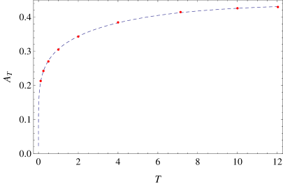
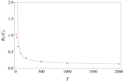
          a.)                                                                         b.)

Figure 6: The running of a.) $A_{T}$ and b.) $B_{T}/C_{T}$ with respect to the temperature. This latter quantity is the position of the pole (cf. (42)). One can see the best matching on higher temperatures.

Let us consider the zero temperature limit:$\lim\limits_{T\rightarrow 0}A_{T}=0$. This tells us that in the zero temperature limit all $\alpha_{ex}$ corresponding to any $\alpha_{2PI}$ by Eq.(38) vanishes. To see this it is easier to invert the relation and then taking the limit, i.e. $\lim_{T\rightarrow 0}A_{T}\ln(\alpha_{2PI}/A_{T}+1)=0$. This is consistent with the fact that at T=0 the coupling drops out from the 2PI propagator Jakovac:2011aa . More precisely at $T=0$ close to the peak:

$${\cal G}_{2PI}(w)\propto\frac{1}{w}\quad\mathrm{,while}\qquad{\cal G}_{ex}(w)\propto\left.\frac{1}{w^{1+\frac{\alpha_{ex}}{\pi}}}\right|_{\alpha_{ex}=0}={\cal G}_{2PI}.$$ (41)

Therefore the diverging $\alpha_{2PI}/\alpha_{ex}$ relation does not signal a physical singularity, it just means that in order to match the exact theory we have to take into account also higher point functions.

The relation in (40) is valid up to the dimensionless temperature $T=12.03$. Above this temperature the trend of the curves can be seen in Fig. 5/a, namely that they are more and more shallow for increasing temperature, changes. The $\alpha_{2PI}(\alpha_{ex})$ curve becomes steeper and steeper as it can be seen in Fig. 5/b. We find for small couplings the expected universal linear relation $\alpha_{2PI}=\alpha_{ex}+\dots$. We can also observe that the $\alpha_{2PI}(\alpha_{ex})$ curves diverge at some limiting value of $\alpha_{ex}$. This can also be seen from the following fit which describes the numerically determined curve quite well:

$$\alpha_{2PI}=\frac{\alpha_{ex}}{B_{T}-C_{T}\alpha_{ex}}.$$ (42)

The fit parameters can be seen in Table 2. This function has a pole at $B_{T}/C_{T}$ at each temperature. This is a temperature dependent quantity, the running of the position of the pole can be seen on Fig. 6/b.

Formula (42) can be interpreted from the point of view of the scale dependence of the coupling constant. For the B-N model the one loop running is exact Jakovac:2011aa , and provides a Landau pole. The value of the coupling where we find the pole is $\alpha(\mu_{0})=\frac{\pi}{\ln\mu/\mu_{0}}$. If we associate $\mu\sim T$ for high temperatures, this would suggest that the finite temperature dependence also exhibits a Landau-type pole at $\alpha_{ex}\sim(\ln fT)^{-1}$. In fact, a two-parameter fit is

$$\frac{B_{T}}{C_{T}}=\frac{d}{\ln(fT),}$$ (43)

where $d=0.576\pm 0.03$ and $f=0.035\pm 0.003$ describes the finite temperature behavior for large temperatures.

The finite temperature running of $\alpha_{2PI}$ for fixed $\alpha_{ex}$ can be seen in Fig. 7.

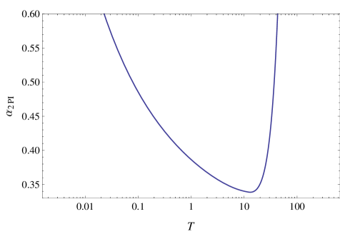
Figure 7: Finite temperature running of $\alpha_{2PI}$ for fixed $\alpha_{ex}$. One can observe the high temperature (Landau) pole and the $T\to 0$ divergence.

According to our earlier analysis we can identify the following characteristic features of this running. For small temperatures the running of the perturbative coupling is determined by the soft IR physics, the photon cloud. At very small temperatures seemingly we find a divergence, but this is not a physical singularity, it just reflects the fact that at zero temperature the 2PI approximation fails to describe the exact spectrum for any couplings, cf. (41). At high temperatures the perturbative running is the dominant effect with the association $\mu\sim T$. Again we find a pole there which comes from the Landau pole of the perturbative running. But again, this singularity is not a physical one, the exact spectrum is regular for $\alpha_{ex}$ larger than the pole value. But with 2PI calculation with the original action we cannot reproduce this result, one would need to take into account higher point vertices, too. Between the low temperature and high temperature regimes there is a point where $d\alpha_{2PI}(T)/dT=0$, in our case this is at the dimensionless temperature value $T=12.03$. This is a “fixed point” of the running and loosely determines a “critical temperature” separating the two physically different temperature regimes.

V.2 The finite velocity case

We can repeat the same analysis for the finite velocity case, too. Since the findings are very similar to the $u=0$ case, we just shortly overview the results.

For the finite velocity case we obtained in our previous article Jakovac:2013aa the following formula in real time:

$$\rho(t)\propto z(t)\rho_{u=0}(t;\alpha_{eff}).$$ (44)

Where we defined an effective coupling which incorporates the information about the finite velocity

$$\alpha_{eff}=\frac{\alpha u_{0}(1-v^{2})}{2v}\ln{\frac{1+v}{1-v}},$$ (45)

and here $v=\frac{u}{u_{0}}$. $z(t)$ is a function of time which is defined as:

$$z(t)=\exp\left\{\frac{u_{0}(1-v^{2})\alpha}{2\pi v}\int\limits_{u_{0}(1-v)}^{u_{0}(1+v)}\!\frac{ds}{s^{2}}\ln\frac{\sinh\pi tTs}{(\sinh\pi Tt)^{s}}\right\}.$$ (46)

In momentum space the product in Eq.(44) turns into a convolution and thus one can derive the finite velocity spectral function only by using numerics. In the 2PI case we are going to use the same numerical calculation that we had for the $u=0$ case, the only difference is that this time we use the formula in Eq.(36) for the discontinuity of the self energy. The spectral functions obtained from 2PI for different $u>0$, but fixed temperature and coupling constant, can be seen on Fig.(8).

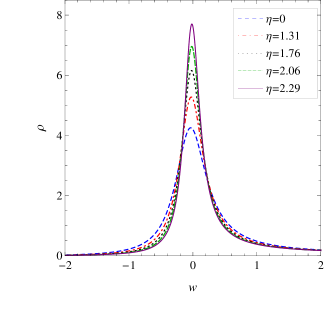
Figure 8: The 2PI spectral functions with different rapidities ($\eta=\tanh^{-1}(v)$, where $v=u/u_{0}$) at fixed temperature $T=1$ and coupling $\alpha=0.5$. The shrinking of the width can be observed as the velocity grows, which is the same effect that we had for the exact solution Jakovac:2013aa .

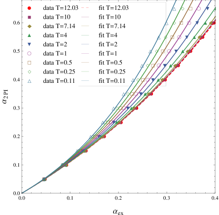
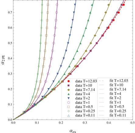
          a.)                                                                             b.)

Figure 9: The relation between the 2PI and the exact coupling for $u=\sqrt{3}$ at temperatures a.) $T\in[0,12.03]$ and b.) $T\in(12.03,\infty)$, respectively. The dashed red line indicates the limiting function at $T=12.03$, for details see the text.

To fit the $u>0$ spectral functions we are applying exactly the same procedure that we used for the $u=0$ case. For this purpose we choose the value $u=\sqrt{3}$ (or $v=\sqrt{3}/2$). In Fig.(9) we can find the relation between the 2PI and the exact couplings and in Table 3, 4 the corresponding fit parameters, but this time for $u=\sqrt{3}$. For the given finite $u$ we have almost the same picture that we had for the $u=0$ case, just the fit parameters, $A_{T},B_{T}$ and $C_{T}$, are different. Interestingly the threshold temperature stayed at $T=12.03$ but the running of the parameter as a function of the temperature is slightly modified. Now we have for $A_{T}=a\tanh(bA_{T})^{c}$, where this time $a=0.55\pm 0.01$, $b=0.075\pm 0.01$ and $c=0.183\pm 0.004$. For the running of the pole we have ($B_{T}/C_{T}=d/\ln(fT)$) $d=0.623\pm 0.04$ and $f=0.032\pm 0.003$.

$T$	$0.11$	$0.25$	$0.5$	$1$	$2$	$4$	$7.14$	$10$	$12.03$
$A_{T}$	$0.235\pm 0.002$	$0.266\pm 0.002$	$0.298\pm 0.002$	$0.338\pm 0.002$	$0.386\pm 0.002$	$0.442\pm 0.002$	$0.488\pm 0.002$	$0.507\pm 0.001$	$0.517\pm 0.001$

Table 3: The fit parameters in the low temperature case for $u=\sqrt{3}$.

$T$	$20$	$50$	$100$	$200$	$500$	$1000$	$2000$
$B_{T}$	$1.016\pm 0.001$	$1.108\pm 0.007$	$1.2\pm 0.014$	$1.29\pm 0.017$	$1.371\pm 0.0175$	$1.389\pm 0.0145$	$1.35\pm 0.009$
$C_{T}$	$0.908\pm 0.002$	$1.422\pm 0.023$	$=2.275\pm 0.048$	$3.629\pm 0.075$	$6.113\pm 0.102$	$8.216\pm 0.105$	$9.8318\pm 0.079$

Table 4: The fit parameters in the high temperature case for $u=\sqrt{3}$.

VI Conclusion

We gave a numerical implementation of the 2PI resummation for the fermionic spectral function in the Bloch-Nordsieck model at non-zero temperature. In our former paper Jakovac:2013aa we showed a derivation of the exact spectral function in an analytic way and obtained a closed form. Hence, this analytic formula provides us a good basis point in the benchmarking of the 2PI. The 2PI technique, being an approximation, cannot provide us a full solution, but we can still compare it to the exact result.

Our first main result is that the 2PI approximation works excellently at finite temperatures, the spectrum coming from the 2PI approximation could be fitted to the exact spectrum with very good accuracy. The two curves could be fitted into each other not just in the vicinity of the peak, but also for much larger momentum interval. This demonstrates that the 2PI resummation is in fact a physically appropriate approximation for gauge theories, too.

Nevertheless, the 2PI and the exact results could be fitted to each other after properly choosing the 2PI coupling $\alpha_{2PI}(\alpha_{ex},T)$ as a function of the coupling of the exact formula ($\alpha_{ex}$) and the temperature. For a fixed $\alpha_{ex}$ this describes a temperature dependent “running” coupling constant. Our second main result is to provide this function for the B-N model.

This temperature dependence has two distinct regimes for small and large temperatures. At small temperatures the deep IR physics dominate the running, the corresponding $\alpha_{2PI}(T)$ decreases with the temperature. For high temperatures the finite temperature running is compatible with the perturbative scale dependence with the choice $\mu\sim T$, there $\alpha_{2PI}(T)$ grows with the temperature. At zero temperature and at some (coupling dependent) high temperatures we find divergences in $\alpha_{2PI}(T)$, in the high temperature case it can be associated with the Landau-pole. But none of these poles mean physical singularity, just the breakdown of the perturbation theory. Between the two regimes there is a temperature, where the temperature derivative of $\alpha_{2PI}^{\prime}(T)=0$. The “critical temperature” of this “fixed point” is in dimensionless units $T=12.03$, this signals the limiting temperature of the soft and perturbative domains.

The success of the 2PI method extended by a nonperturbative running of the coupling constant encourages one to try this strategy also in case of other (gauge) theories. The basis of the temperature running could be the matching of a nonperturbatively (eg. in MC simulations) determined physical quantity. Then, using temperature dependent 2PI couplings one could perform other calculations, and give predictions for other, numerically hardly accessible physical quantities.

- (1) F. Bloch and A. Nordsieck, Phys. Rev. 52 (1937) 54.
- (2) N.N. Bogoliubov and D.V. Shirkov, Introduction to the theories to the quantized fields (John Wiley & Sons, Inc., 1980)
- (3) H.M. Fried, Green’s Functions and Ordered Exponentials (Cambridge University Press, 2002)
- (4) A. Jakovac and P. Mati, Phys. Rev. D 85 (2012) 085006 [arXiv:1112.3476 [hep-ph]].
- (5) J. M. Luttinger and J. C. Ward, Phys. Rev. 118 (1960) 1417. G. Baym, Phys. Rev. 127 (1962) 1391. J. M. Cornwall, R. Jackiw and E. Tomboulis, Phys. Rev. D 10 (1974) 2428, J. Berges and J. Cox, Phys. Lett. B 517 (2001) 369.
- (6) U. Reinosa, J. Serreau, Annals Phys.325:969-1017,2010 [arXiv:0906.2881]
- (7) J. -P. Blaizot and E. Iancu, Phys. Rev. D 55 (1997) 973 [hep-ph/9607303].
- (8) J. -P. Blaizot and E. Iancu, Phys. Rev. D 56 (1997) 7877 [hep-ph/9706397].
- (9) H. M. Fried, T. Grandou and Y. -M. Sheu, Phys. Rev. D 77 (2008) 105027 [arXiv:0804.1591 [hep-th]].
- (10) A. I. Alekseev, V. A. Baikov and E. E. Boos, Theor. Math. Phys. 54, 253 (1983) [Teor. Mat. Fiz. 54, 388 (1983)].
- (11) A. Jakovac and P. Mati, Phys. Rev. D 87 (2013) 125007 [arXiv:1301.1803 [hep-ph]].
- (12) N. P. Landsman and C. G. van Weert, Phys. Rept. 145, 141 (1987); M. Le Bellac, Thermal Field Theory, (Cambridge Univ. Press, 1996.)
- (13) M.E. Peskin, D.V. Schroeder, An Introduction to Quantum Field Theory, (Perseus Books Publishing, 1995.)