The additive model

with different smoothness for the components

Sara van de Geer and Alan Muro

Seminar for Statistics, ETH Zürich

May 26, 2014

Abstract We consider an additive regression model consisting of two components $f^{0}$ and $g^{0}$, where the first component $f^{0}$ is in some sense “smoother” than the second $g^{0}$. Smoothness is here described in terms of a semi-norm on the class of regression functions. We use a penalized least squares estimator $(\hat{f},\hat{g})$ of $(f^{0},g^{0})$ and show that the rate of convergence for $\hat{f}$ is faster than the rate of convergence for $\hat{g}$. In fact, both rates are generally as fast as in the case where one of the two components is known. The theory is illustrated by a simulation study. Our proofs rely on recent results from empirical process theory.

Keywords and phrases. Additive model, oracle rate, penalized least squares, smoothness.

Subject classification. 62G08, 62G05.

1 Introduction

Additive modelling has a long history (Stone (1985), Hastie and Tibshirani (1990)) and is very useful for dealing with the curse of dimensionality. Important estimation methods for such models are for example spline smoothing (Wahba (1990)) or iterative back fitting (Mammen et al. (1999)). Our contribution in this paper is to show that standard spline smoothing or more generally penalized least squares can estimate “smoother” components at a faster rate than “rough” components. In fact, we show an oracle rate for the smoother component, which is as fast as in the case where the rough component is known. Similarly (but perhaps less surprisingly) the rougher component can be estimated as fast as in the case where the smooth component is known. These results are in the same spirit as results for semi-parametric models (Bickel et al. (1998)) saying that the parametric part (the parameter of interest) is estimated with parametric rate despite the presence of an infinite-dimensional nuisance parameter. We make use of recent empirical process theory to deal with an infinite-dimensional parameter of interest.

For simplicity we consider the additive model with two components (extensions to more components can be derived essentially along the same lines). Let $(X_{i},Z_{i})_{i=1}^{n}$ be i.i.d.  input variables and $\{Y_{i}\}_{i=1}^{n}$ be i.i.d. real-valued output variables. The model is

$$Y_{i}=f^{0}(X_{i})+g^{0}(Z_{i})+\epsilon_{i},\ i=1,\ldots,n,$$

where $f^{0}\in{\cal F}$, $g^{0}\in{\cal G}$ with ${\cal F}$ and ${\cal G}$ linear function spaces. Moreover, $\epsilon:=(\epsilon_{1},\ldots,\epsilon_{n})^{T}$ is a vector of i.i.d. centered noise variables, independent of $\{(X_{i},Z_{i})\}_{i=1}^{n}$. For a vector $v\in\mathbb{R}^{n}$ we write $\|v\|_{n}^{2}:=v^{T}v/n$. We study the estimator

$$(\hat{f},\hat{g}):=\arg\min_{f,g}\biggl{\{}\|Y-f-g\|_{n}^{2}+\lambda^{2}I^{2}(f)+\mu^{2}J^{q}(g)\biggr{\}},$$

where $I$ is a semi-norm on ${\cal F}$, $J$ is a semi-norm on ${\cal G}$ and $\lambda$ and $\mu$ are tuning parameters. Moreover, $1\leq q\leq 2$ is some fixed constant. We consider the case where the “smoothness” induced by $I$ is larger than the “smoothness” induced by $J$. For example, when both $X$ and $Z$ are bounded real-valued random variables, one may think of $I$ as being some Sobolev norm, $J$ being the total variation norm and $q=1$. Note that we restrict ourselves to a squared norm in the penalty for the smoother part. A generalization here is straightforward but technical. Also a generalization to values of $q>2$ is not difficult but is omitted to avoid complicated expressions.

We show that with an appropriate choice of the regularization parameters $\lambda$ and $\mu$ the rate of convergence for the smoother function $f^{0}$ is faster than the rate for the less smooth function $g^{0}$. For each component we obtain the rate of convergence corresponding to the situation were the other component is known. This result is established assuming an incoherence condition between $X_{1}$ and $Z_{1}$ (see Condition 2.4).

The results in this paper are related to Wahl (2014). The latter studies an additive two-component model and applies restricted least squares instead of the penalized least squares used here. Another important paper on the topic is Efromovich (2013) where adaptive rates are derived using a method including blockwise shrinkage. Related is also the paper Müller and van de Geer (2013) where a partial linear model is studied with the linear part being high-dimensional. The method used there is penalized least squares with $\ell_{1}$-penalty on the linear part.

1.1 Organization of the paper

In the next section we outline the conditions used. Main condition is an entropy condition (Condition 2.1) which describes the assumed roughness of the functions $f^{0}$ and $g^{0}$. Section 3 contains the main theoretical result in Theorem 3.1. Section 4 presents a simulation study. All proofs are in Section 5.

2 Conditions

Let $P$ be the distribution of $(X,Z)$ and $\|\cdot\|$ be the $L_{2}(P)$-norm. For arbitrary positive constants $R$ and $M$ we let ${\cal F}(R,M):=\{f\in{\cal F}:\ \|f\|\leq R,\ I(f)\leq M\}$ and ${\cal G}(R,M):=\{g\in{\cal G}:\ \|g\|\leq R,\ J(g)\leq M\}$.

Let $\|\cdot\|_{\infty}$ be the supremum norm. The entropy of $({\cal F}(R,M),\|\cdot\|_{\infty})$ is denoted by ${\cal H}_{\infty}(\cdot,{\cal F}(R,M))$. The entropy integral ${\cal J}_{\infty}(\cdot,{\cal F}(R,M))$ is defined as

$${\cal J}_{\infty}(z,{\cal F}(R,M)):=z\int_{0}^{1}\sqrt{{\cal H}_{\infty}(uz,{\cal F}(R,M),\|\cdot\|_{\infty})}du,\ z>0$$

which we assume to exist.

For the class ${\cal G}$ the entropy ${\cal H}_{\infty}(\cdot,{\cal G}(R,M))$ and entropy integral ${\cal J}_{\infty}(\cdot,{\cal G}(R,M))$ are defined similarly. We shall however use a somewhat relaxed version of entropy and entropy integral for ${\cal G}$. Let ${\cal A}_{n}$ be the set of all subsets of cardinality $n$ within the support of $Z_{1}$ (equal points are allowed). For $A_{n}\in{\cal A}_{n}$ and $g$ a real-valued function on this support we let

$$\|g\|_{A_{n},{\infty}}:=\max_{z\in A_{n}}|g(z)|.$$

The entropy of the class $({\cal G}(R,M),\|\cdot\|_{A_{n}})$ endowed with $\|\cdot\|_{A_{n}}$-norm is denoted by ${\cal H}_{A_{n}}(\cdot,{\cal G}(R,M))$. The uniform entropy is

$${\cal H}_{n}(\cdot,{\cal G}(R,M)):=\sup_{A_{n}\in{\cal A}_{n}}{\cal H}_{A_{n}}(\cdot,{\cal G}(R,M)).$$

We furthermore define the entropy integral

$${\cal J}_{n}(z,{\cal G}(R,M)):=z\int_{0}^{1}\sqrt{{\cal H}_{n}(uz,{\cal G}(R,M))}du,\ z>0$$ (1)

assuming again it exists. Note that ${\cal H}_{n}(\cdot,{\cal G}(R,M))\leq{\cal H}_{\infty}(\cdot,{\cal G}(R,M))$ and consequently ${\cal J}_{n}(\cdot,{\cal G}(R,M))\leq{\cal J}_{\infty}(\cdot,{\cal G}(R,M))$.

We fix the “roughness indices” $0<\alpha<\beta<1$ and assume the following bounds on the entropy integrals for ${\cal F}(R,M)$ and ${\cal G}(R,M)$. The reason for the more stringent version of entropy (or entropy integral) for ${\cal F}(R,M)$ is apparent from Lemma 5.3 where we consider for $f\in{\cal F}(R,M)$ conditional versions of $f(X_{1})$ given $Z_{1}$.

Condition 2.1.

For $R\leq M$ and some constants $A_{I}\geq 1$ and $A_{J}\geq 1$, it holds that

$${\cal J}_{\infty}(z,{\cal F}(R,M))\leq A_{I}M^{\alpha}z^{1-\alpha},\ z>0,$$

and

$${\cal J}_{n}(z,{\cal G}(R,M))\leq A_{J}M^{\beta}z^{1-\beta},\ z>0.$$

As an illustration, suppose that $X_{1}\in[0,1]$ and $I^{2}(f)=\int|f^{(k)}(x)|^{2}dx$, where $f^{(k)}$ denotes the $k$-th derivative of $f$. Then $\alpha=1/(2k)$ and the constant $A_{I}$ depends only on the smallest eigenvalue of the matrix ${\rm I\hskip-4.79996ptE}\psi^{T}(X_{1})\psi(X_{1})$ where $\psi(X_{1})=(1,X_{1},\ldots,X_{1}^{k-1})$ (see e.g. Birman and Solomjak (1967)). Similar bounds hold for a general class of Besov spaces, see Birgé and Massart (2000).

We assume $\sup\{\|f\|_{\infty}:\ f\in{\cal F}(R,M)\}$ is bounded by a constant proportional to $M$ and similarly for ${\cal G}(R,M)$. Without loss of generality we assume the proportionality constant to be equal to 1.

Condition 2.2.

For some constant $B\geq 1$ and all $M>0$ and any $R\leq M/B$ it holds that

$$\sup_{f\in{\cal F}(R,M)}\|f\|_{\infty}\leq M,$$

and

$$\sup_{g\in{\cal G}(R,M)}\|g\|_{\infty}\leq M.$$

For a sub-Gaussian random variable $Z\in\mathbb{R}$ and $\Psi(z):=\exp[|z|^{2}]-1$, we define the Orlicz norm

$$\|Z\|_{\Psi}:=\inf\{L>0:{\rm I\hskip-4.79996ptE}\Psi(Z/L)<1\}.$$

We will assume that the noise is sub-Gaussian. Extension to sub-exponential noise is straightforward but omitted to avoid technical digressions.

Condition 2.3.

The error $\epsilon_{1}$ is independent of $(X_{1},Z_{1})$ and satisfies for some constant $K_{\epsilon}\geq 1$

$$\|\epsilon_{1}\|_{\Psi}\leq K_{\epsilon}.$$

Recall that $P$ denotes the distribution of $(X,Z)$. Let $p:=dP/d\nu$ be the density of $P$ with respect to a dominating product measure $\nu:=\nu_{1}\times\nu_{2}$ with marginal densities $p_{1}$ and $p_{2}$. We define

$$r(x,z):={p(x,z)\over p_{1}(x)p_{2}(z)}.$$

We let

$$\gamma^{2}:=\int(r-1)^{2}p_{1}p_{2}d\nu$$

(assumed to exist). Note that $\gamma$ is the $\chi^{2}$-“distance” between the densities $p$ and $p_{1}p_{2}$.

We impose the following incoherence condition.

Condition 2.4.

It holds that $\gamma<1$.

Define

$$f_{\rm P}:=E(f(X_{1})|Z_{1}=\cdot),\ f_{\rm A}:=f-f_{\rm P}.$$

The subscript “${\rm P}$” stands for “projection”, and “${\rm A}$” stands for “anti-projection”. Note that $f_{\rm P}$ is a function with the support of $Z_{1}$ as domain. We assume this function to be smooth.

Condition 2.5.

For some constant $\Gamma$ it holds that

$$J(f_{\rm P})\leq\Gamma\|f\|.$$

To illustrate this condition, suppose that $Z_{1}$ is real-valued and $J(g)=\int|g^{(m)}(z)|dz$. Suppose moreover that

$$\sup_{x}\int|p^{(m)}(x|z)|dz\leq\Gamma,$$

where $p^{(m)}(x|z):={d^{m}\over dz^{m}}(p(x,z)/p_{2}(z))$. Then, interchanging differentiation and integration (and assuming this is allowed)

$$J(f_{\rm P})=\int\biggl{|}\int f(x){p^{(m)}(x|z)}d\nu_{1}(x)\biggr{|}dz\leq\Gamma\int|f(x)|d\nu_{1}(x)\leq\|f\|.$$

3 Main result

We define

$$\tau_{R}(f,g):=\|f+g\|+\lambda I(f)+(\mu/R)^{2-q\over q}\mu J(g).$$ (2)

We moreover let

$$\tau_{I}^{2}(f):=\|f\|^{2}+\lambda^{2}I^{2}(f).$$ (3)

Theorem 3.1.

Assume Conditions 2.1, 2.2, 2.3, 2.4 and 2.5. Suppose that for some $0<\delta<1$, $\max\{A_{I}^{2},A_{J}^{2}\}/n\leq n^{-\delta}$ and $(A_{I}^{2}/n)^{1\over 1+\alpha}\leq(A_{J}^{2}/n)^{1\over 1+\beta}n^{-\delta}$. There exist a universal constant $C$ and constants $c$, $c_{0}$, $c_{1}$, $c_{2}$ depending on $\alpha$, $\beta$, $\gamma$, $\delta$, $B$, $\Gamma$, $q$ and $K_{\epsilon}$ as well as on $I(f^{0})$ and $J(g^{0})$ such that for $n\geq c_{0}$ and

$$\sqrt{n}\lambda^{1+\alpha}=c_{1}A_{I},\ \sqrt{n}\mu^{1+\beta}=c_{1}A_{J},$$

$$R=c_{2}\mu,\ R_{I}=c_{2}\lambda,$$

one has

$${\rm I\hskip-2.20001ptP}\biggl{(}\tau_{R}(\hat{f}-f^{0},\hat{g}-g^{0})\leq R,\ \tau_{I}(\hat{f}-f^{0})\leq R_{I}\biggr{)}\geq 1-C\exp[-n\lambda^{2}/c].$$

The proof is given in Section 5.

Theorem 3.1 does not provide the explicit dependence on the constants. This dependence can in principle be deduced from Lemmas 5.6 and 5.7 albeit that the expressions are somewhat complicated. In an asymptotic formulation, considering $\alpha$, $\beta$, $\gamma$, $\delta$, $B$, $\Gamma$, $q$, $K_{\epsilon}$ as well as $I(f^{0})$ and $J(g^{0})$, as fixed, we get for $\lambda^{2}\asymp A_{I}^{2\over 1+\alpha}n^{-{1\over 1+\alpha}}$ and $\mu^{2}\asymp A_{J}^{2\over 1+\beta}n^{-{1\over 1+\beta}}$, the rates

$$\|\hat{f}-f^{0}\|^{2}={\mathcal{O}}_{{\rm I\hskip-1.54001ptP}}(A_{I}^{2\over 1+\alpha}n^{-{1\over 1+\alpha}}),\ \|\hat{g}-g^{0}\|^{2}={\mathcal{O}}_{{\rm I\hskip-1.54001ptP}}(A_{J}^{2\over 1+\beta}n^{-{1\over 1+\beta}}),$$

$$I(\hat{f})={\mathcal{O}}_{{\rm I\hskip-1.54001ptP}}(1),\ J(\hat{g})={\mathcal{O}}_{{\rm I\hskip-1.54001ptP}}(1).$$

Example 3.1.

Suppose that $X_{1}$ and $Z_{1}$ take values in the interval $[0,1]$ and that $I^{2}(f)=\int|f^{(k)}(x)|^{2}dx$ and $J^{2}(g)=\int|g^{(m)}(z)|^{2}dz$ with $m<k$. Then with $q=2$ the estimator is a spline and easy to calculate as the loss function as well as the penalties are quadratic forms. The rates of convergence are $\|\hat{f}-f^{0}\|={\mathcal{O}}_{{\rm I\hskip-1.54001ptP}}(n^{-{k\over 2k+1}})$ and $\|\hat{g}-g^{0}\|={\mathcal{O}}_{{\rm I\hskip-1.54001ptP}}(n^{-{m\over 2m+1}})$. See Section 4 for some numerical results.

Example 3.2.

Suppose that $X_{1}$ takes its values in $[0,1]$ and $Z_{1}$ is real-valued. Let $I^{2}(f):=\int|f^{(k)}(x)|^{2}dx$ with $k>1$ and $J(g):={\rm TV}(g)$ be the total variation of $g$. Then with $q=1$ the estimator is again easy to calculate (the problem being formally equivalent to a Lasso problem). The rates of convergence are $\|\hat{f}-f^{0}\|={\mathcal{O}}_{{\rm I\hskip-1.54001ptP}}(n^{-{k\over 2k+1}})$ and $\|\hat{g}-g^{0}\|={\mathcal{O}}_{{\rm I\hskip-1.54001ptP}}(n^{-{1\over 3}}\log^{1\over 3}n)$. Indeed, Condition 2.1 for the class ${\cal G}$ now holds with $\beta=1/2$ and $A_{J}\asymp\sqrt{\log n}$. This follows e.g. from Lemma 2.2 in van de Geer (2000). We note that once we have this fast rate for $\|\hat{f}-f^{0}\|$, the $(\log n)$-term in the rate for $\|\hat{g}-g^{0}\|$ can be easily removed using instead of the uniform entropy ${\cal H}_{n}$ the $\|\cdot\|_{n}$-entropy bound from Birman and Solomjak (1967) with $\|\cdot\|_{n}$-being the empirical $L_{2}$-norm (i.e. for a real-valued function $m$ on the support of $(X_{1},Z_{1})$, $\|m\|_{n}:=(\sum_{i=1}^{n}m^{2}(X_{i},Z_{i})/n)^{1/2}$).

4 Simulation results

In this simulation study, we show that the results of Theorem 3.1 also (approximately) hold empirically. We consider Example 3.1. We estimate each of the “true” functions $f^{0}$ and $g^{0}$ in the cases where neither functions are known and the cases where one of them is known. We will see that, for each function, the rate of convergence of the estimator when neither of the “true” functions is known is of the same order than that when one of the components is known. For this, we will show the plots of the MSE of the four estimators in four different scenarios (see Figure 1). However, we will only show the plots of the estimators when correlation$(X,Z)\,=\,0.8$, SNR $=\,7$ since analogous results hold for the other scenarios.

Let $X$ and $U$ be independent uniformly distributed random variables with values in $(0,1)$. Define $Z\,=\,a\,X+(1-a)\,U$ with $a$ an appropriate constant such that the correlation between X and Z is equal to $\rho$ (which we will define later).

We use B-splines of order 6 (piecewise polynomials of degree 5) to represent each of the functions $f$ and $g$ (see de Boor (2001)). We write

$$f(x)=\sum_{i=1}^{K}\gamma_{f,i}b_{f,i}(x),\quad\quad g(z)=\sum_{j=1}^{K}\gamma_{g,j}b_{g,j}(z),$$

where $b_{f,i},b_{g,j},\,\,i,j=1,...,K$ are the basis functions of the B-spline parametrization, $\gamma_{f}=(\gamma_{f,1},...,\gamma_{f,K}),\gamma_{g}=(\gamma_{g,1},...,\gamma_{g,K})$ are the parameters vectors of $f$ and $g$, respectively, and $K+6$ is the number of knots, which we choose to be $\lceil 3\sqrt{n}/5\rceil+6$ where $n$ represents the number of observations. Denote by $(x_{1},...,x_{n})$ and $(z_{1},...,z_{n})$ realizations of the dependent random variables $X$ and $Z$ and let $x_{(r)}$ be the $r$-th order statistic of the sample from $X$ ($r=1,\ldots,n$). For estimating the function $f$ (and analogously for the function $g$), we place the first and last $6$ knots (corresponding to the order of the B-spline) in $x_{(1)}$ and $x_{(n)}$, respectively, and position the remaining knots uniformly in $\{x_{(2)},...,x_{(n-1)}\}$. We define the penalizations as

$$I^{2}(f):=\int_{0}^{1}|f^{\prime\prime\prime}(x)|^{2}\mathrm{d}x\;+\;\int_{0}^{1}|f(x)|^{2}\mathrm{d}x,$$

$$J^{2}(g):=\int_{0}^{1}|g^{\prime\prime}(z)|^{2}\mathrm{d}z\;+\;\int_{0}^{1}|g(z)|^{2}\mathrm{d}z$$

and the $(i,j)-th$ components of the matrices $\Omega_{f},\Omega_{g}\in\mathbb{R}^{K\times K}$ as

$$(\Omega_{f})_{i,j}:=\int_{0}^{1}b_{f,i}^{\prime\prime\prime}(x)b_{f,j}^{\prime\prime\prime}(x)\mathrm{d}x+\int_{0}^{1}b_{f,i}(x)b_{f,j}(x)\mathrm{d}x$$

and

$$(\Omega_{g})_{i,j}:=\int_{0}^{1}b_{g,i}^{\prime\prime}(z)b_{g,j}^{\prime\prime}(z)\mathrm{d}z+\int_{0}^{1}b_{g,i}(z)b_{g,j}(z)\mathrm{d}z$$

Then, we can write $I^{2}(f)=\gamma_{f}^{T}\Omega_{f}\gamma_{f}$ and $J^{2}(g)=\gamma_{g}^{T}\Omega_{g}\gamma_{g}$. Moreover, using Cholesky, we can find matrices $H_{f},H_{g}\in\mathbb{R}^{K\times K}$ such that $\Omega_{f}=H_{f}^{T}H_{f}$ and $\Omega_{g}=H_{g}^{T}H_{g}$.  
 
The case where both $f^{0}$ and $g^{0}$ are unknown:  
Consider the two-components model:

$$Y_{i}=f^{0}(X_{i})+g^{0}(Z_{i})+\epsilon_{i},\quad\quad i=1,...,n,$$ (4)

where $\epsilon_{i},\;i=1,...,n$ are i.i.d. centered Gaussian random variables with variance $\sigma^{2}$. The estimator is

$$(\hat{f},\hat{g}):=\arg\min_{f,g}\biggl{\{}\|Y-f-g\|_{n}^{2}+\lambda^{2}I^{2}(f)+\mu^{2}J^{2}(g)\biggr{\}}.$$

We took $\lambda=14\,n^{-3/7}$ and $\mu=0.3\,n^{-2/5}$. The constants of both tuning parameters are chosen by minimizing the mean square error of the estimators for the case $n=5000$. Candidates for the constants were taken from the grid $(\{1,2,3,...,20\}\times\{0.1,0.2,0.3,...,1\})$, where the first set corresponds to the constant of $\lambda$ and the second to the constant of $\mu$.

The case where $f^{0}$ or $g^{0}$ is known:  
If $g^{0}$ is known we re-write equation (4) as  

$$Y^{f}_{i}=f^{0}(X_{i})+\epsilon_{i},$$

with $Y^{f}_{i}=Y_{i}-g^{0}(Z_{i})$, $i=1,\ldots,n$.

We then use the estimator

$$\hat{f}^{s}:=\arg\min_{f}\biggl{\{}\|Y^{f}-f\|_{n}^{2}+\lambda^{2}I^{2}(f)\biggr{\}}.$$

The tuning parameter is taken to be $\lambda=14\,n^{-3/7}$.

Similarly, if $f^{0}$ is known we let $Y^{g}:=Y-f^{0}$ and

$$\hat{g}^{s}:=\arg\min_{g}\biggl{\{}\|Y^{g}-g\|_{n}^{2}+\mu^{2}J^{2}(g)\biggr{\}}$$

with $\mu=0.3\,n^{-2/5}$.

Simulations:  
Define the Signal-to-Noise ratio as ${\rm SNR}:={\rm var}(f^{0}(X)+g^{0}(Z))/{\sigma^{2}}$. For our simulations, we consider the following scenarios:

• $f^{0}(x)=-10\sin(1.9x+0.2\pi)+\mathbb{E}[10\sin(1.9x+0.2\pi)]$.

• $g^{0}(z)=3e^{-500(z-0.1)^{2}}-\mathbb{E}[3e^{-500(z-0.1)^{2}}]$.

• SNR $\in\{0.5,7\}$.

• $\rho\,\in\,\{0.2,0.8\}$.

• $n\in\{100,150,200,...,5000\}$.

The error variance $\sigma^{2}$ was chosen in each scenario to match the above given Signal-to -Noise ratios. For each $n$ the average of 100 simulations is used to estimate the mean square error. In Figure 1, we see that the rate of convergence of $\hat{f}$ and of $\hat{f}^{s}$ are of similar order and that the same applies to $\hat{g}^{s}$ and $\hat{g}$. In other words, for each function $f^{0}$ and $g^{0}$, the rate of convergence of the estimators when both functions are unknown (approximately) corresponds to the case when one of them is known. These results agree with Theorem 3.1 and hold in the four simulation scenarios. Moreover, we see that the convergence of $\hat{f}^{s}$ and $\hat{f}$ to $f^{0}$ is faster than that of $\hat{g}^{s}$ and $\hat{g}$ to $g^{0}$, which is also established in Theorem 3.1.

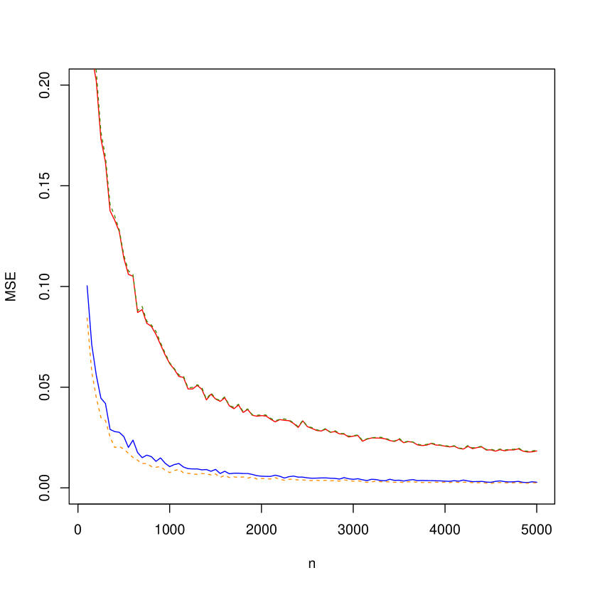
(a) $\rho\,=\,0.2$, SNR = 0.5

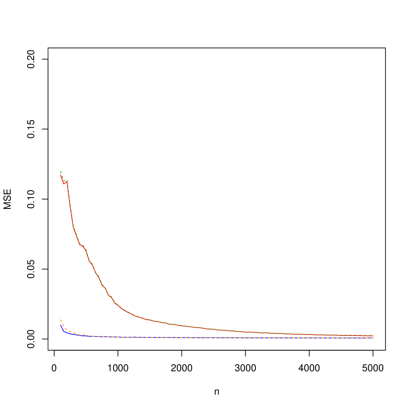
(b) $\rho\,=\,0.2$, SNR = 7

(c) $\rho\,=\,0.8$, SNR = 0.5

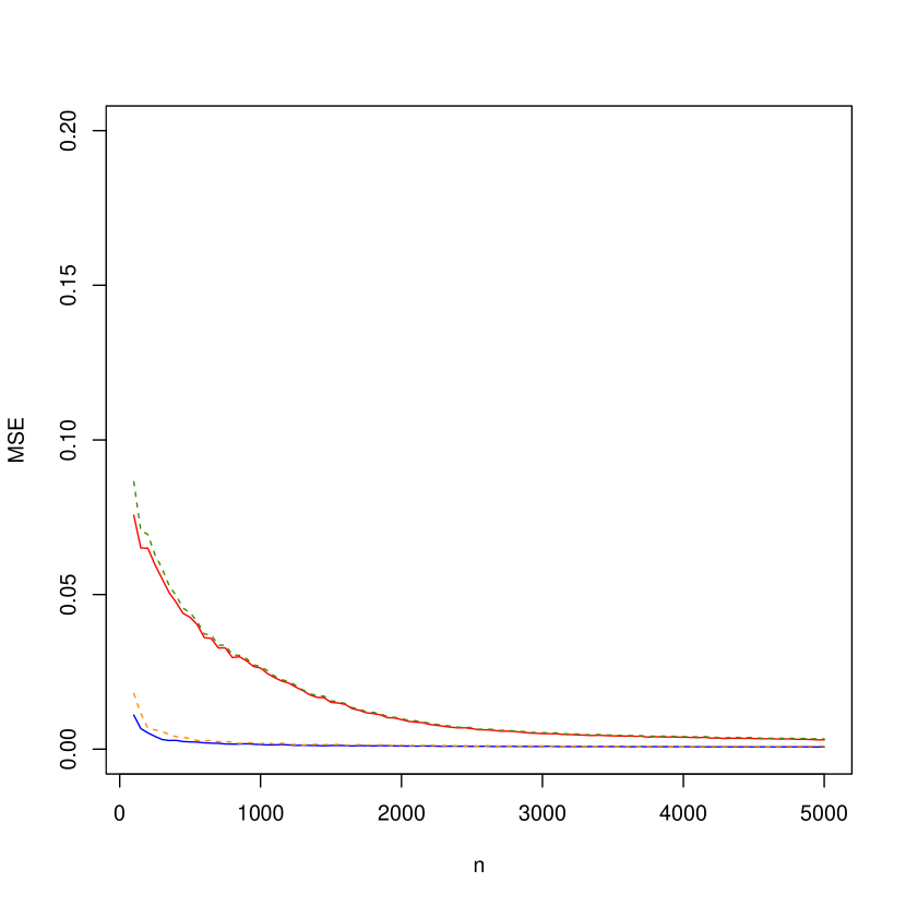
(d) $\rho\,=\,0.8$, SNR=7

Figure 1: Estimated MSE for each of the computed estimators: $\hat{f}^{s}$ (blue line), $\hat{g}^{s}$ (red line), $\hat{f}$ (orange dotted line), and $\hat{g}$ (green dotted line) for the four simulation scenarios.

The log-transformed data from Figure 1 for the scenario $\rho\,=\,0.8$ and SNR = 7 is plotted in Figure 2. Here, we fit a linear regression on each curve considering only those observations corresponding to $n\,\geq\,1000$ and print the slope of these and the theoretical slope in the legend of the plot. With SNR=7 it is not clear whether the slopes of the regression line of the estimators agree with their theoretical counterpart. For lower SNR however the agreement is remarkably good (not shown here).

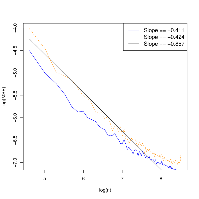
(a) Log transformed data for $\hat{f}^{s}$ (blue line) and $\hat{f}$ (orange dotted line)

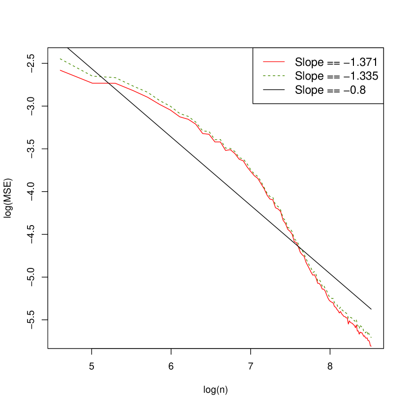
(b) Log transformed data for $\hat{g}^{s}$ (red line) and $\hat{g}$ (green dotted line)

Figure 2: Log-transformed data for the case $\rho\,=\,0.8$ and SNR = 7. A black line using the theoretical slope and an arbitrary intercept was drawn for graphical comparison.

The plots of both $f^{0}$ and $g^{0}$ and their corresponding estimators for the scenario $\rho\,=\,0.8$ and SNR = 7 are displayed in Figure 3. We can see that, as the number of observations increases, the functions $\hat{f}$ and $\hat{g}$ converge to $\hat{f}^{s}$ and $\hat{g}^{s}$, respectively. This happens while all of them improve their estimation of the true functions $f^{0}$ and $g^{0}$ appropriately. We note that $\hat{f}$ and $\hat{f}^{s}$ are almost identical to $f^{0}$ when the number of observations is large. However, $\hat{g}$ and $\hat{g}^{s}$ can only resemble but not describe perfectly $g^{0}$. This is probably due to the highly variable second and third derivatives of $g^{0}$ in comparison with those of $f^{0}$, as can be seen in Figure 4.

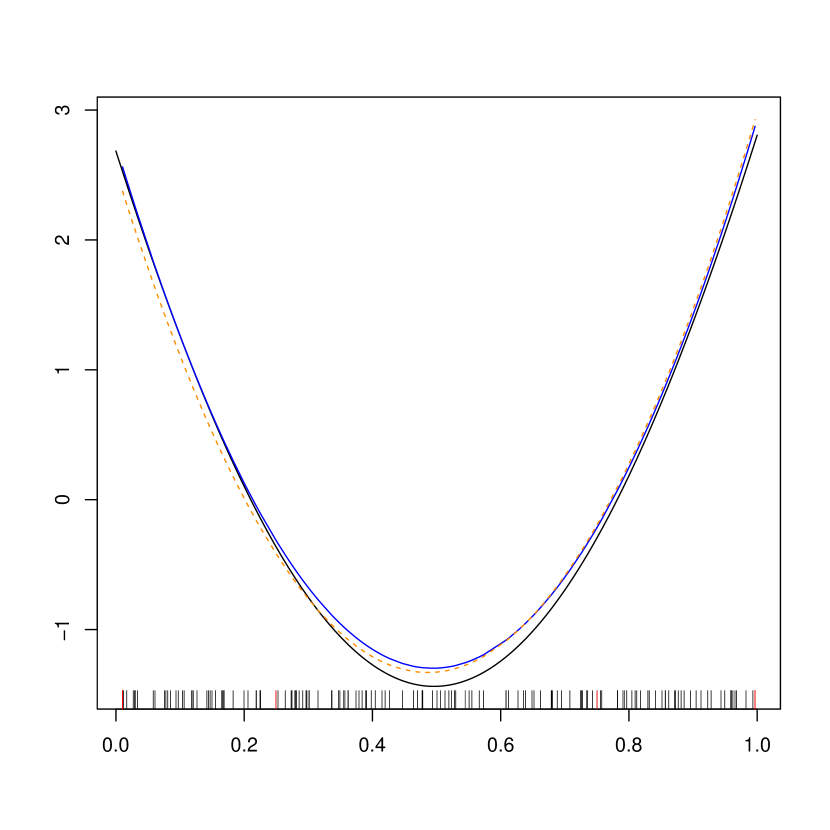
(a) $n$ = 150

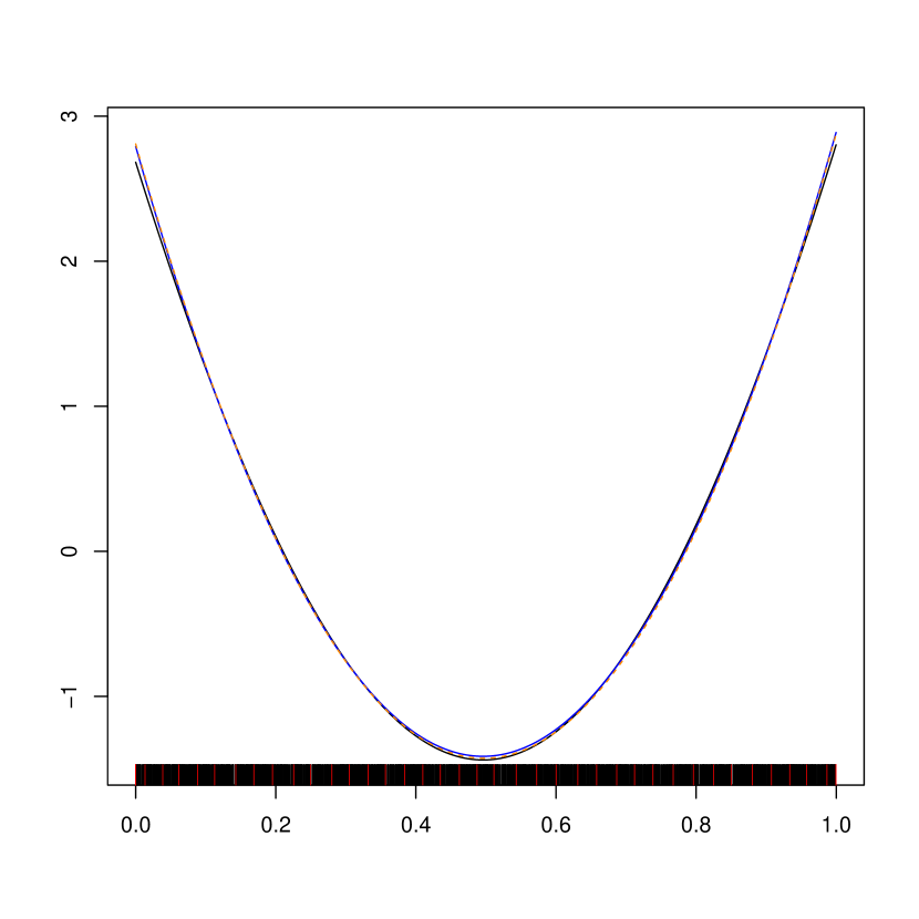
(b) $n$ = 5000

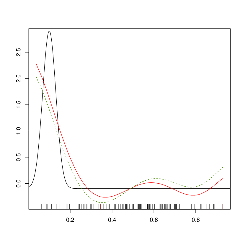
(c) $n$ = 150

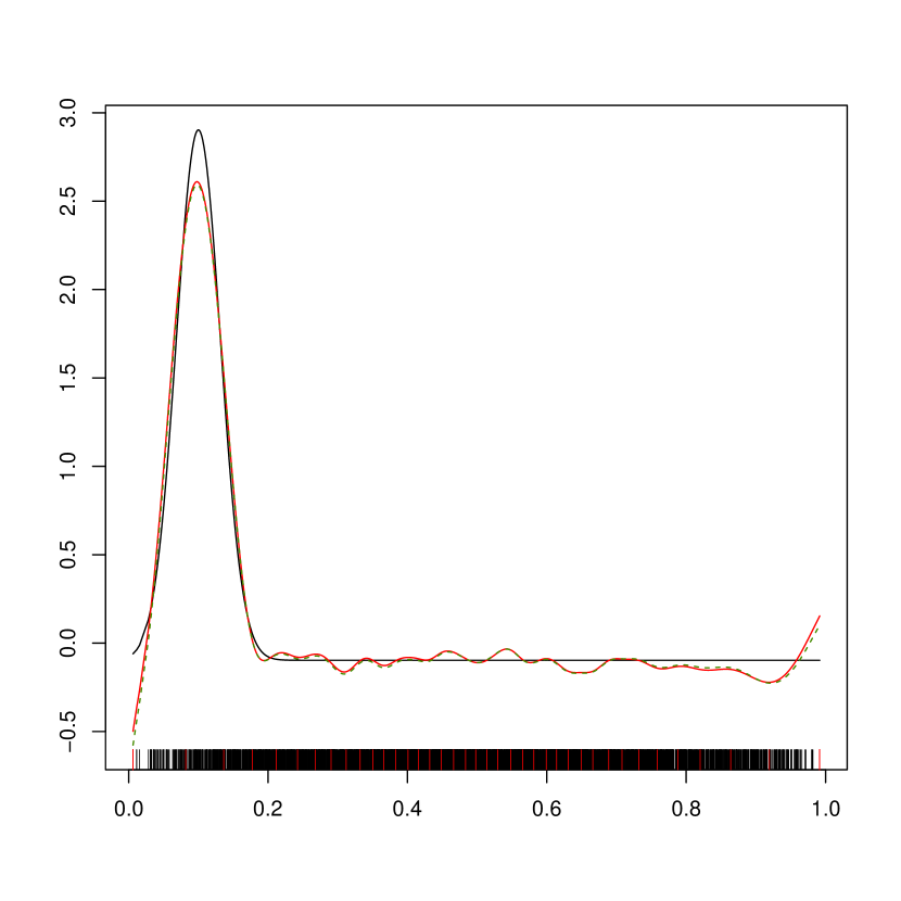
(d) $n$ = 5000

Figure 3: Plots of the true functions $f^{0}$ and $g^{0}$ (black lines) with their corresponding estimators $\hat{f}^{s}$ (blue lines), $\hat{f}$ (orange dotted lines), $\hat{g}^{s}$ (red lines), $\hat{g}$ (green dotted lines), for $\rho\,=\,0.8$ and SNR = 7. The data are represented with black small vertical lines and knots positions with red small vertical lines. For each $n\in\{150,5000\}$, we use a single simulation (not 100 simulations).

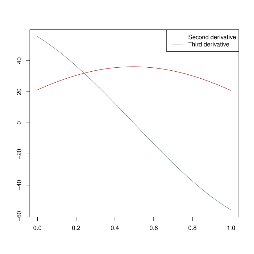
(a) Derivatives of $f^{0}$.

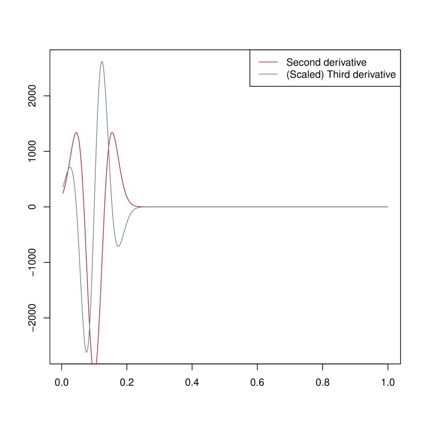
(b) Derivatives of $g^{0}$.

Figure 4: Second and third derivatives of the true functions $f^{0}$ and $g^{0}$ in $[0,1]$. The third derivative of $g^{0}$ was multiplied by 0.02 for an easier comparison.

5 Proofs

We use the notation $P_{n}:=\sum_{i=1}^{n}\delta_{(X_{i},Z_{i})}/n$ for the empirical measure based on $\{(X_{i},Z_{i})\}_{i=1}^{n}$.

The proof is organized as follows. We first present some preliminary results needed for the proof of the faster rate for $\hat{f}$. Then we look in Subsection 5.2 at the global rate for both components. We use here the convexity of the least squares loss function and the penalties to localize the problem to the set ${\cal M}(R):=\{(f,g):\ \tau_{R}(f,g)\leq R\}$, and then show that indeed $(\hat{f}-f^{0},\hat{g}-g^{0})\in{\cal M}(R)$ provided that the random part of the problem is under control. In Subsection 5.5 we show the random part is indeed under control with large probability. For this result, we need recent findings from empirical process theory, in particular the convergence of empirical norms and inner products. Here, we apply some results from van de Geer (2014). The application is somewhat elaborate: for an additive model with $p$ components there are ${p+1\choose 2}-1$ terms to consider. If there is only one component, say $f$, one needs to consider the behaviour of $\|f\|_{n}^{2}-\|f\|^{2}$ and $\epsilon^{T}f/n$ uniformly over some collection of functions $f$. If there are two components $f$ and $g$ the number of terms to consider is five: namely uniform convergence $\|f\|_{n}^{2}$, $\|g\|_{n}^{2}$, $P_{n}fg$, $\epsilon^{T}f/n$ and $\epsilon^{T}g/n$ to their theoretical counterparts. This is done in Subsection 5.4. Subsection 5.2 takes such uniform convergence for granted. The same is true in Subsection 5.3 where we show the faster rate for the estimator $\hat{f}$ of the smoother component: the results are on a random event which is shown to have large probability in Subsection 5.6 using results from empirical process theory given in Subsection 5.4. We finally collect all pieces in Subsection 5.7 to finish the proof of the main result in Theorem 3.1.

5.1 Preliminaries

Lemma 5.1.

Assume Condition 2.4 and suppose $\int fp_{1}d\nu_{1}=0$. Then

$$\|f+g\|^{2}\geq(1-\gamma)(\|f\|+\|g\|)^{2}.$$

Proof. We have

$$\|f+g\|^{2}=\|f\|^{2}+\|g\|^{2}+2\int(fg)pd\nu.$$

Moreover, since $\int fp_{1}=0$,

$$|\int fgpd\nu|=|\int fg(r-1)p_{1}p_{2}d\nu|\leq\gamma(\int f^{2}g^{2}p_{1}p_{2}d\nu)^{1/2}=\gamma\|f\|\|g\|.$$

Hence,

$$\|f+g\|^{2}\geq\|f\|^{2}+\|g\|^{2}-2\gamma\|f\|\|g\|$$

$$=(1-\gamma)(\|f\|^{2}+\|g\|^{2})+\gamma(\|f\|-\|g\|)^{2}\geq(1-\gamma)(\|f\|+\|g\|)^{2}.$$

$\sqcup\mkern-12.0mu\sqcap$

Lemma 5.2.

Assume Condition 2.4 and suppose $\int fp_{1}d\nu_{1}=0$. We have that

$$\|f_{\rm P}\|^{2}\leq\gamma\|f\|^{2}$$

and

$$\|f_{\rm A}\|^{2}\geq(1-\gamma^{2})\|f\|^{2}.$$

Proof. We have

$$f_{\rm P}=\int f(r-1)p_{1}d\nu_{1}.$$

Hence

$$\|f_{\rm P}\|\leq\|r-1\|\|f\|=\gamma\|f\|,$$

and

$$\|f_{\rm A}\|^{2}=\|f\|^{2}-\|f_{\rm P}\|^{2}\geq(1-\gamma^{2})\|f\|^{2}.$$

$\sqcup\mkern-12.0mu\sqcap$.

Lemma 5.3.

Assume Conditions 2.1 and 2.2. Then

$${\cal J}_{\infty}(z,\{f_{\rm A}:\ f\in{\cal F}(R,M)\})\leq 2{\cal J}_{\infty}(z,{\cal F}(R,M)),\ z>0$$

and for $R\leq M/B$

$$\sup_{f\in{\cal F}(R,M)}\|f_{\rm A}\|_{\infty}\leq 2M.$$

Proof. Let $u>0$ and $f,\ \tilde{f}\in{\cal F}(R,M)$ be arbitrary, satisfying $\|f-\tilde{f}\|_{\infty}\leq u$. Then clearly also

$$\|f_{\rm P}-\tilde{f}_{\rm P}\|_{\infty}=\|E(f(X_{1})-\tilde{f}(X_{1})|Z=\cdot)\|_{\infty}\leq u.$$

So then

$$\|f_{\rm A}-\tilde{f}_{\rm A}\|_{\infty}\leq\|f_{\rm P}-\tilde{f}_{\rm P}\|_{\infty}+\|f-\tilde{f}\|_{\infty}\leq 2u.$$

Similarly, for $f\in{\cal F}(R,M)$, we have

$$\|f_{\rm A}\|_{\infty}\leq\|f_{\rm P}\|_{\infty}+\|f\|_{\infty}\leq 2M.$$

$\sqcup\mkern-12.0mu\sqcap$

5.2 A global bound

We define

$${\cal M}(R):=\{(f,g):\ \tau_{R}(f,g)\leq R\}$$ (5)

and for a sufficiently small value $\delta_{0}>0$, to be chosen later the sets

$${\cal T}_{1}(R):=\biggl{\{}\sup_{(f,g)\in{\cal M}(R)}\biggl{|}\|f+g\|_{n}^{2}-\|f+g\|^{2}\biggr{|}\leq\delta_{0}^{2}R^{2}\biggr{\}},$$

$${\cal T}_{2}(R):=\biggl{\{}\sup_{(f,g)\in{\cal M}(R)}|\epsilon^{T}(f+g)|/n\leq\delta_{0}^{2}R^{2}\biggr{\}},$$

and

$${\cal T}(R):={\cal T}_{1}(R)\cap{\cal T}_{2}(R).$$ (6)

Lemma 5.4.

Take $\delta_{0}\leq{1\over 20}$ and suppose that

$$\lambda^{2}I^{2}(f^{0})+\mu^{2}J^{q}(g^{0})\leq\delta_{0}^{2}R^{2}.$$ (7)

Then on ${\cal T}(R)$, we have $\|\hat{m}-m^{0}\|^{2}+\lambda^{2}I^{2}(\hat{f})+\mu^{2}J^{q}(\hat{g})\leq 4\delta_{0}^{2}R^{2}$ and $\tau_{R}(\hat{f}-f^{0},\hat{g}-g^{0})\leq R$.

Proof. Define

$$\tilde{f}:=t\hat{f}+(1-t)f^{0},\ \tilde{g}:=t\hat{g}+(1-t)g^{0}$$

with

$$t:={R\over R+\tau_{R}(\hat{f}-f^{0},\hat{g}-g^{0})}.$$

Then $\tau_{R}(\tilde{f}-f^{0},\tilde{g}-g^{0})\leq R$. Let $\tilde{m}:=\tilde{f}+\tilde{g}$ and $m^{0}:=f^{0}+g^{0}$. By convexity

$$\|\tilde{m}-m^{0}\|_{n}^{2}+\lambda^{2}I^{q}(\tilde{f})+\mu^{2}J^{q}(\tilde{g})\leq 2\epsilon^{T}(\tilde{m}-m^{0})+\lambda^{2}I^{q}(f^{0})+\mu^{2}J^{q}(g^{0}).$$

On ${\cal T}(R)$ we find

$$\|\tilde{m}-m^{0}\|^{2}+\lambda^{2}I^{q}(\tilde{f})+\mu^{2}J^{q}(\tilde{g})\leq 4\delta_{0}^{2}R^{2}.$$

Hence

$$I(\tilde{f})\leq(2\delta_{0})R/\lambda,$$

and

$$J(\tilde{g})\leq(2\delta_{0})^{2/q}(R/\mu)^{2/q}\leq 2\delta_{0}(R/\mu)^{2/q}$$

where in the last step we used $2\delta_{0}<1$ and $2/q\geq 1$. Since by (7) it holds that $I(f^{0})\leq 2\delta_{0}R/\lambda$ we get

$$I(\tilde{f}-f^{0})\leq 4\delta_{0}R/\lambda.$$

Also, by (7) we have $J(g^{0})\leq(2\delta_{0})^{2/q}(R/\mu)^{2/q}\leq 2\delta_{0}(R/\mu)^{2/q}$ so that

$$J(\tilde{g}-g^{0})\leq 4\delta_{0}(R/\mu)^{2/q}.$$

We find

$$\lambda I(\tilde{f}-f^{0})\leq 4\delta_{0}R$$

as well as

$$(\mu/R)^{2-q\over q}\mu J(\tilde{g}-g^{0})\leq 4\delta_{0}R.$$

But then

$$\tau_{R}(\tilde{f}-f^{0},\tilde{g}-g^{0})=\|\tilde{m}-m^{0}\|+\lambda I(\tilde{f}-f^{0})+(\mu/R)^{2-q\over q}\mu J(\tilde{g}-g^{0})$$

$$\leq 10\delta_{0}R\leq R/2$$

where we used $\delta_{0}\leq{1\over 20}$. This implies $\tau_{R}(\hat{f}-f^{0},\hat{g}-g^{0})\leq R$. Repeating the argument completes the proof. $\sqcup\mkern-12.0mu\sqcap$

5.3 A tighter bound for the smoother part

Let ${\cal F}(R_{I}):=\biggl{\{}f:\ \tau_{I}(f)\leq R_{I}\biggr{\}}.$

For $\delta_{1}$ sufficiently small we define

$${\cal T}_{1,I}(R_{I}):=\biggl{\{}\sup_{f\in{\cal F}(R_{I})}\biggl{|}\|f_{A}\|_{n}^{2}-\|f_{A}\|^{2}\biggr{|}\leq\delta_{1}^{2}R_{I}^{2}\biggr{\}},$$

$${\cal T}_{I,2}(R_{I}):=\biggl{\{}\sup_{f\in{\cal F}(R_{I})}|\epsilon^{T}f_{A}|/n\leq\delta_{1}^{2}R_{I}^{2}\biggr{\}},$$

$${\cal T}_{I,3}(R_{I},R):=\biggl{\{}\sup_{(f,g)\in{\cal M}(R):\ f\in{\cal F}(R_{I})}|P_{n}f_{A}(g+f_{P})|\leq\delta_{1}^{2}R_{I}^{2}\biggr{\}}$$

and we let

$${\cal T}_{I}(R_{I},R):={\cal T}_{I,1}(R_{I})\cap{\cal T}_{I,2}(R_{I})\cap{\cal T}_{I,3}(R_{I},R).$$ (8)

Lemma 5.5.

Assume Condition 2.4 and 2.5. Suppose the condition (7)

$$\lambda^{2}I^{2}(f^{0})+\mu^{2}J^{2}(g^{0})\leq\delta_{0}^{2}R^{2}$$

of Lemma 5.4 holds, with $\delta_{0}\leq{1\over 20}$ given as there. Suppose moreover that

$$\lambda^{2}I^{2}(f^{0})\leq\delta_{1}^{2}R_{I}^{2},$$ (9)

$$2\mu^{2}\Gamma(2\delta_{0}R/\mu)^{2(q-1)\over q}\leq\delta_{1}^{2}R_{I}^{2},\ 2\mu^{2}\Gamma^{q}/R_{I}^{2-q}\leq\delta_{1}^{2}$$ (10)

and ${\delta_{1}^{2}}\leq{(1-\gamma^{2})\over 36}$. Then on ${\cal T}(R)\cap{\cal T}_{I}(R_{I})$ it holds that $\tau_{I}(\hat{f}-f^{0})\leq R_{I}$.

Proof. We use the Basic Inequality

$$\|Y-\hat{f}-\hat{g}\|_{n}^{2}+\lambda^{2}I^{2}(\hat{f})+\mu^{2}J^{q}(\hat{g})\leq\|Y-f^{0}-(\hat{g}+\hat{f}_{\rm P}-f_{\rm P}^{0})\|_{n}^{2}$$

$$+\lambda^{2}I^{2}(f^{0})+\mu^{2}J^{q}(\hat{g}+\hat{f}_{\rm P}-f_{\rm P}^{0}).$$

This gives that

$$\|\hat{f}_{\rm A}-f_{\rm A}^{0}\|^{2}+\lambda^{2}I^{2}(\hat{f})+\mu^{2}J^{q}(\hat{g})$$

$$\leq 2\epsilon^{T}(\hat{f}_{\rm A}-f_{\rm A}^{0})/n-2(\hat{f}_{\rm A}-f_{\rm A}^{0})^{T}(\hat{g}-g^{0}+\hat{f}_{\rm P}-f_{\rm P}^{0})/n$$

$$+\|\hat{f}_{\rm A}-f_{\rm A}^{0}\|^{2}-\|\hat{f}_{\rm A}-f_{\rm A}^{0}\|_{n}^{2}+\lambda^{2}I^{2}(f^{0})+\mu^{2}J^{q}(\hat{g}+\hat{f}_{\rm P}-f_{\rm P}^{0}).$$

By convexity the inequality also holds if we replace $\hat{f}$ by $\tilde{f}:=t\hat{f}+(1-t)\hat{f}^{0}$ with

$$t:={R_{I}\over R_{I}+\tau_{I}(\hat{f}-f^{0})}.$$

Before exploiting this, we derive a bound for $J^{q}(\hat{g}+\tilde{f}_{\rm P}-f_{\rm P}^{0})$. We use that for positive $a$ and $b$,

$$(a+b)^{q}-a^{q}\leq 2(a+b)^{q-1}b\leq 2(a^{q-1}+b^{q-1})b=2a^{q-1}b+2b^{q}$$

Hence

$$J^{q}(\hat{g}+\tilde{f}_{\rm P}-f_{\rm P}^{0})-J^{q}(\hat{g})\leq 2J^{q-1}(\hat{g})J(\tilde{f}_{\rm P}-f_{\rm P}^{0})+2J^{q}(\tilde{f}_{\rm P}-f_{\rm P}^{0})$$

$$\leq 2\Gamma J^{q-1}(\hat{g})\|\tilde{f}-f^{0}\|+2\Gamma^{q}\|\tilde{f}-f^{0}\|^{q}$$

where in the last step we used Condition 2.5. On ${\cal T}(R)$ we have $J(\hat{g})\leq(2\delta_{0}R/\mu)^{2/q}$ by Lemma 5.4. We also have $\|\tilde{f}-f^{0}\|\leq R_{I}$. Hence

$$J^{q}(\hat{g}+\tilde{f}_{\rm P}-f_{\rm P}^{0})-J^{q}(\hat{g})\leq 2\Gamma(2\delta_{0}R/\mu)^{2(q-1)\over q}R_{I}+2\Gamma^{q}R_{I}^{q}.$$

But then by condition (10)

$$\mu^{2}J^{q}(\hat{g}+\tilde{f}_{\rm P}-f_{\rm P}^{0})\leq 2\delta_{1}^{2}R_{I}^{2}.$$

We insert this result in the Basic Inequality with $\hat{f}$ replaced by $\tilde{f}$:

$$\|\tilde{f}_{\rm A}-f_{\rm A}^{0}\|^{2}+\lambda^{2}I^{2}(\tilde{f})\leq 6\delta_{1}^{2}R_{I}^{2}+\lambda^{2}I^{2}(f_{0}).$$

Invoking (9) we get

$$\|\tilde{f}_{\rm A}-f_{\rm A}^{0}\|^{2}+\lambda^{2}I^{2}(\tilde{f}-f_{0})\leq 6\delta_{1}^{2}R_{I}^{2}+3\lambda^{2}I^{2}(f^{0})\leq 9\delta_{1}^{2}R_{I}^{2}.$$

Since by Lemma 5.2 $\|\tilde{f}-f^{0}\|^{2}\geq\|\tilde{f}_{A}-f_{A}^{0}\|^{2}/(1-\gamma^{2})$, this implies

$$\tau_{I}^{2}(\tilde{f}-f^{0})\leq 9\delta_{1}^{2}R_{I}^{2}/(1-\gamma^{2})\leq R_{I}^{2}/4$$

using $\delta_{1}^{2}\leq{(1-\gamma^{2})\over 36}$. This implies $\tau_{I}(\hat{f}-f^{0})\leq R_{I}$.

$\sqcup\mkern-12.0mu\sqcap$

5.4 Results from empirical process theory

We use Theorem 2.1 in van de Geer (2014) which is a consequence of results in Guédon et al. (2007) and combine this with Theorem 3.1. in van de Geer (2014). We recall definition (1) of the entropy integral ${\cal J}_{n}$. Throughout, $C_{0}$ and $C_{1}$ are universal constants.

Theorem 5.1.

Fix some $R_{1}$, $M_{1}$, $R_{2}$ and $M_{2}$ and let

$$K_{1}:=\sup_{f\in{\cal F}(R_{1},M_{1})}\|f\|_{\infty},\ K_{2}:=\sup_{g\in{\cal G}(R_{2},M_{2})}\|g\|_{\infty}.$$

Define for all $t$ and $n$

$$B_{1,1}(t,n):={R_{1}{\cal J}_{n}(K_{1},{\cal F}(R_{1},M_{1}))+R_{1}K_{1}\sqrt{t}\over\sqrt{n}}+{{\cal J}_{n}^{2}(K_{1},{\cal F}(R_{1},M_{1}))+K_{1}^{2}t\over n},$$

$$B_{2,2}(t,n):={R_{2}{\cal J}_{n}(K_{2},{\cal G}(R_{2},M_{2}))+R_{2}K_{2}\sqrt{t}\over\sqrt{n}}+{{\cal J}_{n}^{2}(K_{2},{\cal G}(R_{2},M_{2}))+K_{2}^{2}t\over n}$$

and

$$B_{1,2}(t,n):={R_{1}{\cal J}_{n}(K_{2},{\cal G}(R_{2},M_{2}))+R_{2}{\cal J}_{n}(R_{1}K_{2}/R_{2},{\cal F}(R_{1},M_{1}))\over\sqrt{n}}$$

$$+{R_{1}K_{2}\sqrt{t}\over\sqrt{n}}+{K_{1}K_{2}t\over n}.$$

We have for all $t>0$ with probability at least $1-C_{0}\exp[-t]$

$$\sup_{f\in{\cal F}(R_{1},M_{1})}\biggl{|}\|f\|_{n}^{2}-\|f\|^{2}\biggr{|}\leq C_{1}B_{1,1}(t,n),\ \sup_{g\in{\cal G}(R_{2},M_{2})}\biggl{|}\|g\|_{n}^{2}-\|g\|^{2}\biggr{|}\leq C_{1}B_{2,2}(t,n).$$

Moreover, for $R_{1}K_{2}\leq R_{2}K_{1}$ and all values of $t$ and $n$ satisfying

$$C_{1}B_{1,1}(t,n)\leq{R_{1}^{2}},\ C_{1}B_{2,2}(t,n)\leq{R_{2}^{2}}$$

we have with probability at least $1-C_{0}\exp[-t]$

$$\sup_{f\in{\cal F}(R_{1},M_{1}),\ g\in{\cal G}(R_{2},M_{2})}\biggl{|}(P_{n}-P)fg\biggr{|}\leq C_{1}B_{1,2}(t,n).$$

The next result follows from standard arguments using Dudley’s results (Dudley (1967)), see e.g. van der Vaart and Wellner (1996).

Theorem 5.2.

Assume Condition 2.3 on the noise. Fix some $R_{1}$, $M_{1}$, $R_{2}$ and $M_{2}$ and let

$$K_{1}:=\sup_{f\in{\cal F}(R_{1},M_{1})}\|f\|_{\infty},\ K_{2}:=\sup_{g\in{\cal G}(R_{2},M_{2})}\|g\|_{\infty}.$$

Consider values of $t$ and $n$ such that

$$C_{1}B_{1,1}(t,n)\leq{R_{1}^{2}},\ C_{1}B_{2,2}(t,n)\leq{R_{2}^{2}}$$

with $B_{1,1}(t,n)$ and $B_{2,2}(t,n)$ given in Theorem 5.1. For these values, with probability at least $1-C_{0}\exp[-t]$, one has

$$\sup_{f\in{\cal F}(R_{1},M_{1})}|\epsilon^{T}f|/n\leq C_{1}B_{1,\epsilon}(t,n),\ \sup_{g\in{\cal G}(R_{2},M_{2})}|\epsilon^{T}g|/n\leq C_{1}B_{2,\epsilon}(t,n),$$

where

$$B_{1,\epsilon}(t,n):={K_{\epsilon}{\cal J}(R_{1},{\cal F}(R_{1},M_{1}))+K_{\epsilon}R_{1}\sqrt{t}\over\sqrt{n}}$$

and

$$B_{2,\epsilon}(t,n):={K_{\epsilon}{\cal J}(R_{2},{\cal G}(R_{2},M_{2}))+K_{\epsilon}R_{2}\sqrt{t}\over\sqrt{n}}.$$

Corollary 5.1.

Suppose Conditions 2.1, 2.2 and 2.3. Assume $R_{1}\leq M_{1}/B$ and $R_{2}\leq M_{2}/B$ where the constant $B$ is from Condition 2.2. Let $B_{1,1}$, $B_{2,2}$, $B_{1,2}$ be defined as in Theorem 5.1 and $B_{1,\epsilon}$ and $B_{2,\epsilon}$ be defined as in Theorem 5.2. Then

$$B_{1,1}(t,n)\leq{R_{1}M_{1}(A_{I}+\sqrt{t})\over\sqrt{n}}+{M_{1}^{2}(A_{I}^{2}+t)\over n},$$

$$B_{2,2}(t,n)\leq{R_{2}M_{2}(A_{J}+\sqrt{t})\over\sqrt{n}}+{M_{2}^{2}(A_{J}^{2}+t)\over n}.$$

$$B_{1,2}(t,n)\leq{A_{J}R_{1}M_{2}+A_{I}R_{2}^{\alpha}R_{1}^{1-\alpha}M_{1}^{\alpha}M_{2}^{1-\alpha}\over\sqrt{n}}+{R_{1}M_{2}\sqrt{t}\over\sqrt{n}}+{M_{1}M_{2}t\over n}$$

and

$$B_{1,\epsilon}(t,n)\leq{A_{I}K_{\epsilon}M_{1}^{\alpha}R_{1}^{1-\alpha}+K_{\epsilon}R_{1}\sqrt{t}\over\sqrt{n}},\ B_{2,\epsilon}(t,n)\leq{A_{J}K_{\epsilon}M_{2}^{\beta}R_{2}^{1-\beta}+K_{\epsilon}R_{2}\sqrt{t}\over\sqrt{n}}.$$

The constants $A_{I}$ and $A_{J}$ are from Condition 2.1 and the constant $K_{\epsilon}$ from Condition 2.3.

Theorem 5.3.

Assume Conditions 2.1, 2.2 and 2.3. Let $\lambda\leq R_{I}\leq\mu\leq R\leq 1$ be constants and $L_{I}:=R_{I}/\lambda$ and $L_{J}:=(R/\mu)^{2/q}$.
Case 1. Assume $\lambda^{2}\leq 1/B^{2}$ and $\mu^{2}\leq R^{2-q}/B^{q}$. Suppose that for some $L\geq 4C_{1}$,

$$\sqrt{n}\lambda^{1+\alpha}\geq LA_{I},\ \sqrt{n}\mu^{1+\beta}\geq LA_{J},$$ (11)

$$R\geq LL_{J}A_{J}/\sqrt{n},\ R\geq K_{\epsilon}\lambda,\ R\geq L_{J}\lambda,\ R\geq K_{\epsilon}^{q\over q-(2-q)\beta}\mu$$ (12)

and

$$\lambda^{\alpha}\leq 1/L.$$ (13)

Then with probability at least $1-3C_{0}\exp[-n\lambda^{2}/L^{2}]$ it holds that

$$\sup_{f\in{\cal F}(R,R/\lambda)}\biggl{|}\|f\|_{n}^{2}-\|f\|^{2}\biggr{|}\leq{4R^{2}\over L},\ \sup_{g\in{\cal G}(R,L_{J})}\biggl{|}\|g\|_{n}^{2}-\|g\|^{2}\biggr{|}\leq{4R^{2}\over L},$$

$$\sup_{f\in{\cal F}(R,R/\lambda),\ g\in{\cal G}(R,L_{J})}\biggl{|}(P_{n}-P)fg\biggr{|}\leq{4R^{2}\over L}$$

and

$$\sup_{f\in{\cal F}(R,R/\lambda)}|\epsilon^{T}f|/n\leq{2R^{2}\over L},\ \sup_{g\in{\cal G}(R,L_{J})}|\epsilon^{T}g|/n\leq{2R^{2}\over L}.$$

Case 2. Assume moreover that

$$R_{I}\geq LL_{J}A_{J}/\sqrt{n},\ R_{I}\geq K_{\epsilon}\lambda$$ (14)

Then with probability at least $1-3C_{0}\exp[-n\lambda^{2}/L^{2}]$,

$$\sup_{f\in{\cal F}(R_{I},L_{I})}\biggl{|}\|f\|_{n}^{2}-\|f\|^{2}\biggr{|}\leq{4R_{I}^{2}\over L},\ \sup_{f\in{\cal F}(R_{I},L_{I}),\ g\in{\cal G}(R,L_{J})}\biggl{|}(P_{n}-P)fg\biggr{|}\leq{4R_{I}^{2}\over L}$$

and

$$\sup_{f\in{\cal F}(R_{I},L_{I})}|\epsilon^{T}f|/n\leq{2R_{I}^{2}\over L}.$$

Proof of Theorem 5.3.

Case 1. We first apply Corollary 5.1 with $R_{1}=R_{2}=R$ and $M_{1}=R/\lambda$, $M_{2}=L_{J}:=(R/\mu)^{2/q}$. The condition $\lambda\leq 1/B$ ensures $R_{1}\leq M_{1}/B$ and the condition $\mu\leq R^{2-q\over q}/B$ ensures that $R_{2}\leq M_{2}/B$. We let $B_{1,1}$, $B_{2,2}$, $B_{1,2}$ be defined as in Theorem 5.1 and $B_{1,\epsilon}$ and $B_{2,\epsilon}$ be defined as in Theorem 5.2 and insert the value $t=n\lambda^{2}/L^{2}$.

Case 1a for $\|f\|_{n}^{2}$.

$$B_{1,1}(t,n)\leq{R^{2}(A_{I}+\sqrt{t})\over\sqrt{n}\lambda}+{R^{2}(A_{I}^{2}+t)\over n\lambda^{2}}=\biggl{(}{A_{I}+\sqrt{t}\over\sqrt{n}\lambda}+{A_{I}^{2}+t\over n\lambda^{2}}\biggr{)}R^{2}.$$

Now use that by (11) $\sqrt{n}\lambda\geq LA_{I}$ and $t=n\lambda^{2}/L^{2}$ to get

$$B_{1,1}(t,n)\leq\biggl{(}{2\over L}+{2\over L^{2}}\biggr{)}\leq{4R^{2}\over L}$$

Case 1b For $\|g\|_{n}^{2}$.

$$B_{2,2}(t,n)\leq{RL_{J}(A_{J}+\sqrt{t})\over\sqrt{n}}+{L_{J}^{2}(A_{J}^{2}+t)\over n}=\biggl{(}{L_{J}(A_{J}+\sqrt{t})\over\sqrt{n}R}+{L_{J}^{2}(A_{J}^{2}+t)\over nR^{2}}\biggr{)}R^{2}$$

$$\leq\biggl{(}{1\over L}+{\sqrt{t}\over\sqrt{n}R}+{1\over L^{2}}+{t\over nR^{2}}\biggr{)}R^{2},$$

where we used that $R\geq LL_{J}A_{J}/\sqrt{n}$ by (12). Insert $R\geq\lambda$ and $t=n\lambda^{2}/L^{2}$ to get

$$B_{2,2}(t,n)\leq\biggl{(}{2\over L}+{2\over L^{2}}\biggr{)}R^{2}\leq{4R^{2}\over L}.$$

Case 1c for $f^{T}g/n$. We already know by Cases 1a and 1b that $C_{1}B_{1,1}(t,n)\leq R^{2}$ and $C_{1}B_{2,2}(t,n)\leq R^{2}$ with probability at least $1-C_{0}\exp[-n\lambda^{2}/L^{2}]$. Moreover

$$B_{1,2}(t,n)\leq{RL_{J}A_{J}+R^{1+\alpha}L_{J}^{1-\alpha}A_{I}/\lambda^{\alpha}+RL_{J}\sqrt{t}\over\sqrt{n}}+{RL_{J}t\over n\lambda}$$

$$=\biggl{(}{L_{J}A_{J}\over\sqrt{n}R}+{L_{J}^{1-\alpha}A_{I}\lambda\over\sqrt{n}R^{1-\alpha}\lambda^{1+\alpha}}+{L_{J}\sqrt{t}\over\sqrt{n}R}+{L_{J}t\over nR\lambda}\biggr{)}{R^{2}}.$$

Use $R\geq\lambda L_{J}$, $R\geq LL_{J}A_{J}/\sqrt{n}$ from (12) and $\sqrt{n}\lambda^{1+\alpha}\geq LA_{I}$ from (11) to find that

$$B_{1,2}(t,n)\leq\biggl{(}{1\over L}+\lambda^{\alpha}+{\sqrt{t}\over\sqrt{n}\lambda}+{t\over n\lambda^{2}}\biggr{)}{R^{2}}.$$

Apply now that by (13) $\lambda^{\alpha}\leq 1/L$ and $t=n\lambda^{2}/L^{2}$ to get

$$B_{1,2}(t,n)\leq\biggl{(}{3\over L}+{1\over L^{2}}\biggr{)}\leq{4R^{2}\over L}.$$

Case 1d for $\epsilon^{T}f/n$. We already know by Cases 1a and 1b that $C_{1}B_{1,1}(t,n)\leq R^{2}$ and $C_{1}B_{2,2}(t,n)\leq R^{2}$ with probability at least $1-C_{0}\exp[-n\lambda^{2}/L^{2}]$. Moreover

$$B_{1,\epsilon}(t,n)\leq{K_{\epsilon}A_{I}\lambda R\over\sqrt{n}\lambda^{1+\alpha}}+{K_{\epsilon}R\sqrt{t}\over\sqrt{n}}=\biggl{(}{K_{\epsilon}A_{I}\lambda\over\sqrt{n}\lambda^{1+\alpha}R}+{K_{\epsilon}\sqrt{t}\over\sqrt{n}R}\biggr{)}R^{2}.$$

Invoke $\sqrt{n}\lambda^{1+\alpha}\geq LA_{I}$ from (11) and $R\geq K_{\epsilon}\lambda$ from (12) to obtain

$$B_{1,\epsilon}(t,n)\leq\biggl{(}{1\over L}+{\sqrt{t}\over\sqrt{n}\lambda}\biggr{)}R^{2}.$$

With $t=n\lambda^{2}/L^{2}$ this gives

$$B_{1,\epsilon}(t,n)\leq{2R^{2}\over L}.$$

Case 1e for $\epsilon^{T}g/n$. We gave

$$B_{2,\epsilon}(t,n)\leq\biggl{(}{K_{\epsilon}A_{J}L_{J}^{\beta}\over\sqrt{n}R^{1+\beta}}+{K_{\epsilon}\sqrt{t}\over\sqrt{n}R}\biggr{)}R^{2}.$$

Use $\sqrt{n}\mu^{1+\beta}\geq LA_{J}$ from (11) to find

$$B_{2,\epsilon}(t,n)\leq\biggl{(}{L_{J}^{\beta}(\mu/R)^{1+\beta}K_{\epsilon}\over L}+{K_{\epsilon}\sqrt{t}\over\sqrt{n}R}\biggr{)}R^{2}.$$

Next, we see that $L_{J}^{\beta}(\mu/R)^{1+\beta}\leq 1/K_{\epsilon}$ since $R\geq K_{\epsilon}^{q\over q-(2-q)\beta}\mu$ by (12). Moreover, also by (12) $R\geq K_{\epsilon}\lambda$. So with $t=n\lambda^{2}/L^{2}$

$$B_{2,\epsilon}(t,n)\leq\biggl{(}{1\over L}+{\sqrt{t}\over\sqrt{n}\lambda}\biggr{)}R^{2}={2R^{2}\over L}.$$

Case 2. Take $R_{1}=R_{I}$, $R_{2}=R$ and $M_{1}=L_{I}$, $M_{2}=L_{J}$. Then again $R_{1}\leq M_{1}/B$ and $R_{2}\leq M_{2}/B$. Also With these new values, we let $B_{1,1}$, $B_{2,2}$, $B_{1,2}$ be defined as in Theorem 5.1 and $B_{1,\epsilon}$ and $B_{2,\epsilon}$ be defined as in Theorem 5.2 and insert the value $t=n\lambda^{2}/L^{2}$.

Case 2a for $\|f\|_{n}^{2}$.

$$B_{1,1}(t,n)\leq{R_{I}^{2}(A_{I}+\sqrt{t})\over\sqrt{n}\lambda}+R_{I}^{2}{A_{I}^{2}+t\over n\lambda^{2}}=\biggl{(}{A_{I}+\sqrt{t}\over\sqrt{n}R_{I}}+{A_{I}+t\over nR_{I}^{2}}\biggr{)}R_{I}^{2}\leq{4R_{I}^{2}/L}$$

since $\sqrt{n}R_{I}\geq\sqrt{n}\lambda\geq\sqrt{n}\lambda^{1+\alpha}\geq LA_{I}$ by (11) and $t=n\lambda^{2}/L^{2}$.

Case 2b for $f^{T}g/n$. By similar arguments as in Case 1a (see also Case 2a) and 1b that $C_{1}B_{1,1}(t,n)\leq R_{I}^{2}$ and $C_{2}B_{2,2}(t,n)\leq R^{2}$ with probability at least $1-C_{0}\exp[-n\lambda^{2}/L^{2}]$. Moreover

$$B_{1,2}(t,n)\leq{R_{I}L_{J}A_{J}\over\sqrt{n}}+{R^{\alpha}R_{I}\lambda L_{J}^{1-\alpha}A_{I}\over\sqrt{n}\lambda^{1+\alpha}}+{R_{I}L_{J}\sqrt{t}\over\sqrt{n}}+{tR_{I}L_{J}\over n\lambda}$$

$$=\biggl{(}{L_{J}A_{J}\over\sqrt{n}R_{I}}+{R^{\alpha}\lambda L_{J}^{1-\alpha}A_{I}\over\sqrt{n}\lambda^{1+\alpha}R_{I}}+{L_{J}\sqrt{t}\over\sqrt{n}R_{I}}+{tL_{J}\over n\lambda R_{I}}\biggr{)}R_{I}^{2}.$$

Use that $R_{I}\geq LL_{J}A_{J}/\sqrt{n}$ (see (14)), $\sqrt{n}\lambda^{1+\alpha}\geq LA_{I}$ (see (11)) and $R\geq\lambda L_{J}$ (see (12)). We then get

$$B_{1,2}(t,n)\leq\biggl{(}{1\over L}+\lambda^{\alpha}+{\sqrt{t}\over\sqrt{n}\lambda}+{t\over n\lambda^{2}}\biggr{)}R_{I}^{2}.$$

With $t=n\lambda^{2}/L^{2}$ and $\lambda^{\alpha}\leq 1/L$ (see (13)) this gives again

$$B_{1,2}(t,n)\leq{4R_{I}^{2}\over L}.$$

Case 2c for $\epsilon^{T}f/n$. By Case 2a, it holds that $C_{1}B_{1,1}(t,n)\leq R_{I}^{2}$ with probability at least $1-C_{0}\exp[-n\lambda^{2}/L^{2}]$. Moreover

$$B_{1,\epsilon}(t,n)\leq\biggl{(}{K_{\epsilon}A_{I}\lambda\over\sqrt{n}\lambda^{1+\alpha}R_{I}}+{K_{\epsilon}\sqrt{t}\over\sqrt{n}R_{I}}\biggr{)}R_{I}^{2}.$$

From (11) we know $\sqrt{n}\lambda^{1+\alpha}\geq LA_{I}$ and from (14) $R_{I}\geq K_{\epsilon}\lambda$. With $t=n\lambda^{2}/L^{2}$ we find

$$B_{1,\epsilon}(t,n)\leq{2R_{I}^{2}\over L}.$$

The result now follows from the same arguments as in Case 2 of Theorem 5.3.

$\sqcup\mkern-12.0mu\sqcap$

Remark 5.1.

If we assume condition (11), then condition (12) is met for

$$K_{\epsilon}{\lambda\over\mu}\leq K_{\epsilon}^{q\over q-(2-q)\beta}\leq{R\over\mu}\leq{\rm min}\biggl{\{}\biggl{(}{\sqrt{n}\over LA_{J}}\biggr{)}^{q\beta\over(1+\beta)(2-q)},\biggl{(}{\mu\over\lambda}\biggr{)}^{q\over 2-q}\biggr{\}}.$$

Under general conditions, the left hand side tends to zero and the right hand side tends to infinity as $n\rightarrow\infty$.

5.5 Application to ${\cal T}(R)$

Recall the definition (6) of the set ${\cal T}(R)$.

Lemma 5.6.

Let $\lambda\leq\mu\leq R\leq 1$. Assume Conditions 2.1, 2.2, 2.3 and 2.4. Assume that $\lambda^{2}\leq(1-\gamma)/B^{2}$ and $\mu^{2}\leq(1-\gamma)^{q}R^{2-q}/B^{q}$. Let

$$L\geq\max\biggl{\{}4C_{1}(1-\gamma)^{1/2},16/((1-\gamma)^{1/2}\delta_{0}^{2})\biggr{\}}$$

and

$$\sqrt{n}\lambda^{1+\alpha}\geq LA_{I},\ \sqrt{n}\mu^{1+\beta}\geq LA_{J},$$

$$\lambda^{\alpha}\leq(1-\gamma)^{1+\alpha\over 2}/L$$

and

$$K_{\epsilon}{\lambda\over\mu}\leq K_{\epsilon}^{q\over q-(2-q)\beta}\leq{R\over\mu}\leq{\rm min}\biggl{\{}\biggl{(}{\sqrt{n}(1-\gamma)^{1/2}\over LA_{J}}\biggr{)}^{q\beta\over(1+\beta)(2-q)},\biggl{(}{\mu\over\lambda}\biggr{)}^{q\over 2-q}\biggr{\}}.$$

Then

$${\rm I\hskip-2.20001ptP}({\cal T}(R))\geq 1-\exp[-n\lambda^{2}/L^{2}].$$

Proof. Recall the definition of ${\cal M}(R)$ given in (5) with $\tau_{R}(\cdot,\cdot)$ given in (2). Define $\tilde{\lambda}^{2}:=\lambda^{2}/(1-\gamma)$, $\tilde{\mu}^{2}:=\mu^{2}/(1-\gamma)$ and $\tilde{R}^{2}:=R^{2}/(1-\gamma)$. By Lemma 5.1

$${\cal M}(R)\subset\biggl{\{}(f,g):\ \|f\|\leq\tilde{R},\ \|g\|\leq\tilde{R},\ I(f)\leq R/\lambda,\ J(g)\leq(R/\mu)^{2\over q}\biggr{\}}$$

$$=\biggl{\{}(f,g):\ f\in{\cal F}(\tilde{R},\tilde{R}/\tilde{\lambda}),\ g\in{\cal G}(\tilde{R},(\tilde{R}/\tilde{\mu})^{2\over q}\biggr{\}}.$$

We apply Case 1 of Theorem 5.3 with $(\lambda,\mu,R)$ replaced by $(\tilde{\lambda},\tilde{\mu},\tilde{R})$. We also replace $L$ by $\tilde{L}^{2}:=L^{2}/(1-\gamma)$. Then

$$\sqrt{n}\tilde{\lambda}^{1+\alpha}=\sqrt{n}\lambda^{1+\alpha}/(1-\gamma)^{1+\alpha\over 2}$$

$$\geq LA_{I}/(1-\gamma)^{1+\alpha\over 2}=\tilde{L}A_{I}/(1-\gamma)^{\alpha\over 2}\geq\tilde{L}A_{I}.$$

Similarly

$$\sqrt{n}\tilde{\mu}^{1+\beta}\geq\tilde{L}A_{J}.$$

The condition $\lambda^{\alpha}\leq(1-\gamma)^{1+\alpha\over 2}/L$ gives

$$\tilde{\lambda}^{\alpha}={\lambda^{\alpha}\over(1-\gamma)^{\alpha/2}}\leq{(1-\gamma)^{1+\alpha\over 2}\over L(1-\gamma)^{\alpha\over 2}}={1\over\tilde{L}}.$$

Furthermore

$$K_{\epsilon}{\tilde{\lambda}\over\tilde{\mu}}\leq K_{\epsilon}^{q\over q-(2-q)\beta}\leq{\tilde{R}\over\tilde{\mu}}\leq{\rm min}\biggl{\{}\biggl{(}{\sqrt{n}\over\tilde{L}A_{J}}\biggr{)}^{q\beta\over(1+\beta)(2-q)},\biggl{(}{\tilde{\mu}\over\tilde{\lambda}}\biggr{)}^{q\over 2-q}\biggr{\}}.$$

By Remark 5.1 we conclude that the conditions for Case 1 of Theorem 5.3 are met. Clearly, for any $f$ and $g$

$$\biggl{|}\|f+g\|_{n}^{2}-\|f+g\|^{2}\biggr{|}\leq\biggl{|}\|f\|_{n}^{2}-\|f\|_{n}^{2}\biggr{|}+\biggl{|}\|g\|_{n}^{2}-\|g\|^{2}\biggr{|}+\biggl{|}2(P_{n}-P)fg\biggr{|}.$$

By Case 1 of Theorem 5.3, for $\tilde{L}=L/(1-\gamma)^{1/2}\geq 4C_{1}$ and for $16\tilde{R}^{2}/\tilde{L}\leq\delta_{0}^{2}R^{2}$

$${\rm I\hskip-2.20001ptP}({\cal T}(R))\geq 1-\exp[-n\tilde{\lambda}^{2}/\tilde{L}^{2}].$$

The proof if finished by noting that $\tilde{R}^{2}/\tilde{L}=R^{2}/(L(1-\gamma)^{1/2})$ and $\tilde{\lambda}^{2}/\tilde{L}^{2}=\lambda^{2}/L^{2}$.

$\sqcup\mkern-12.0mu\sqcap$

5.6 Application to ${\cal T}_{I}(R_{I})$

Recall the definition (8) of the set ${\cal T}_{I}(R_{I},R)$.

Lemma 5.7.

Assume Conditions 2.1, 2.2, 2.3, 2.4 and 2.5. Let $\lambda\leq R_{I}\leq\mu\leq R\leq 1$. Assume that $\lambda^{2}\leq(1-\gamma)/(2B)^{2}$ and $\mu^{2}\leq(1-\gamma)^{q}R^{2-q}/(2B)^{q}$. Let

$$L\geq\max\biggl{\{}2C_{1}(1-\gamma)^{1/2},32/((1-\gamma)^{1/2}\delta_{0}^{2}),32/(\delta_{1}^{2})\biggr{\}}.$$

Take

$$\sqrt{n}\lambda^{1+\alpha}\geq LA_{I},\ \sqrt{n}\mu^{1+\beta}\geq LA_{J},$$

$$\lambda^{\alpha}\leq(2(1-\gamma))^{1+\alpha\over 2}/L$$

and

$$K_{\epsilon}{\lambda\over\mu}\leq K_{\epsilon}^{q\over q-(2-q)\beta}\leq{R\over\mu}\leq{\rm min}\biggl{\{}\biggl{(}{\sqrt{n}(1-\gamma)^{1/2}\over 2LA_{J}}\biggr{)}^{q\beta\over(1+\beta)(2-q)},\biggl{(}{\mu\over\lambda}\biggr{)}^{q\over 2-q}\biggr{\}}.$$

Also take

$$R_{I}\geq L(R/\mu)^{2\over q}A_{J}/\sqrt{n},\ R_{I}\geq K_{\epsilon}\lambda$$

$$\Gamma R_{I}\leq(2R/\mu)^{2\over q}$$

Then

$${\rm I\hskip-2.20001ptP}({\cal T}_{I}(R_{I},R))\geq 1-3C_{0}\exp[-n\lambda^{2}/L^{2}].$$

Proof. By Lemma 5.3

$${\cal J}_{\infty}(z,\{f_{\rm A}:\ f\in{\cal F}(R,M)\})\leq 2{\cal J}_{\infty}(z,{\cal F}(R,M)),\ z>0$$

and for $R\leq M/B$

$$\sup_{f\in{\cal F}(R,M)}\|f_{\rm A}\|_{\infty}\leq 2M.$$

We can therefore apply similar arguments as for Case 2 of Theorem 5.3. We know that for $f\in{\cal F}(R_{I})$, $\|f_{\rm A}\|\leq\|f\|\leq R_{I}$. So

$${\cal J}_{\infty}(z,\{f_{\rm A}:\ f\in{\cal F}(R_{I})\})\leq 2{\cal J}_{\infty}(z,{\cal F}(R_{I},R_{I}/\lambda)),\ z>0$$

and

$$\sup_{f\in{\cal F}(R_{I})}\|f_{\rm A}\|_{\infty}\leq 2R_{I}/\lambda.$$

Moreover, for $f\in{\cal F}(R_{I})$ and $g\in{\cal G}(R)$ we have

$$J(g+f_{\rm P})\leq J(g)+J(f_{\rm P})\leq(R/\mu)^{2/q}+\Gamma\|f\|\leq(R/\mu)^{2/q}+\Gamma R_{I}\leq(2R/\mu)^{2/q},$$

and

$$\|g+f_{\rm P}\|\leq\|g\|+\|f_{\rm P}\|\leq R/(1-\gamma)^{1/2}+R_{I}\leq 2R/(1-\gamma)^{1/2}.$$

It follows that

$$\{g+f_{\rm P}:\ f\in{\cal F}(R_{I}),\ g\in{\cal G}(R)\}\subset{\cal G}(2R/(1-\gamma)^{1/2},(2R/\mu)^{2/q}).$$

It is also clear that for any $f$ and $g$

$$Pf_{\rm A}g=Ef(X_{1})g(Z_{1})-E\biggl{[}E(f(X_{1})|Z)g(Z_{1})\biggr{]}=0$$

and similarly $Pf_{\rm A}f_{\rm P}=0$. By an appropriate replacements of the constants in Case 2 of Theorem 5.3 (as in the proof of Lemma (5.6) now using $(1-\gamma)^{1/2}/2$ instead of $(1-\gamma)^{1/2}$) the results follows.

$\sqcup\mkern-12.0mu\sqcap$

5.7 Finishing the proof of Theorem 3.1

We first note that since $\max\{A_{I},A_{J}\}\leq n^{1-\delta\over 2}$ we $\lambda^{1+\alpha}=c_{1}A_{I}/\sqrt{n}\leq n^{-\delta/2}$. So for $n$ large $\lambda$ will be small. The same is true for $\mu$ and for the ratio $\lambda/\mu$.

In view of Lemma 5.4 we need $\lambda^{2}I^{2}(f^{0})+\mu^{2}J^{q}(g^{0})\leq\delta_{0}^{2}R^{2}$. We take

$$R^{2}=\max\biggl{\{}\mu^{2}J^{q}(g^{0})/(4\delta_{0}^{2}),K_{\epsilon}^{2q\over 2-(2-q)\beta}\biggr{\}}$$

and $n$ sufficiently large such that

$$\lambda^{2}I^{2}(f^{0})\leq\mu^{2}J^{q}(g^{0}).$$

Take

$$L=\max\biggl{\{}2C_{1}(1-\gamma)^{1/2},32/((1-\gamma)^{1/2}\delta_{0}^{2}),32/(\delta_{1}^{2})\biggr{\}}.$$

Since

$$\max\biggr{\{}{J^{q/2}(g^{0})\over 2\delta_{0}},K_{\epsilon}^{q\over 2-(2-q)\beta}\biggr{\}}\leq{\rm min}\biggl{\{}\biggl{(}{\sqrt{n}(1-\gamma)^{1/2}\over 2LA_{J}}\biggr{)}^{q\beta\over(1+\beta)(2-q)},\biggl{(}{\mu\over\lambda}\biggr{)}^{q\over 2-q}\biggr{\}}$$

for $n$ sufficiently large as $A_{J}\leq n^{1-\delta\over 2}$ we know from Remark 5.1 that the conditions for Lemma 5.6 are met for $n$ sufficiently large. By Lemma 5.5 we also need $\lambda^{2}I^{2}(f_{0})\leq R_{I}^{2}/\delta_{1}^{2}$. For $R_{I}/\lambda=\max\{I(f^{0})/\delta_{1},K_{\epsilon}\}$.

$$R_{I}\geq L(R/\mu)^{2\over q}A_{J}/\sqrt{n}$$

for $n$ sufficiently large so we can also apply Lemma 5.7.

References

- Bickel et al. [1998] P.J. Bickel, C.A.J. Klaassen, Y. Ritov, and J.A. Wellner. Efficient and Adaptive Estimation for Semiparametric Models. Springer, 1998.
- Birgé and Massart [2000] L. Birgé and P. Massart. An Adaptive Compression Algorithm in Besov Spaces. Constructive Approximation, 16(1):1–36, 2000.
- Birman and Solomjak [1967] M.Š. Birman and M.Z. Solomjak. Piecewise-polynomial approximations of functions of the classes . Mathematics of the USSR-Sbornik, 2:295–317, 1967.
- de Boor [2001] C. de Boor. A Practical Guide to Splines. 2001 Revised Edition. Springer-Verlag, New-York, 2001.
- Dudley [1967] R.M. Dudley. The sizes of compact subsets of hilbert space and continuity of gaussian processes. Journal of Functional Analysis, 1:290–330, 1967.
- Efromovich [2013] S. Efromovich. Nonparametric regression with the scale depending on auxiliary variable. The Annals of Statistics, 41(3):1542–1568, 2013.
- Guédon et al. [2007] O. Guédon, S. Mendelson, A. Pajor, and N. Tomczak-Jaegermann. Subspaces and orthogonal decompositions generated by bounded orthogonal systems. Positivity, 11:269–283, 2007.
- Hastie and Tibshirani [1990] T.J. Hastie and R.J. Tibshirani. Generalized Additive Models, volume 43. CRC Press, 1990.
- Mammen et al. [1999] E. Mammen, O. Linton, and J. Nielsen. The existence and asymptotic properties of a backfitting projection algorithm under weak conditions. The Annals of Statistics, 27(5):1443–1490, 1999.
- Müller and van de Geer [2013] P. Müller and S. van de Geer. The partial linear model in high dimensions, 2013. arXiv:1307.1067, tentatively accepted by Scandinavian Journal of Statistics.
- Stone [1985] C.J. Stone. Additive regression and other nonparametric models. The Annals of Statistics, pages 689–705, 1985.
- van de Geer [2000] S. van de Geer. Empirical Processes in M-Estimation. Cambridge University Press, 2000.
- van de Geer [2014] S. van de Geer. On the uniform convergence of empirical norms and inner products, with application to causal inference. Electronic Journal of Statistics, 8:543–574, 2014.
- van der Vaart and Wellner [1996] A. W. van der Vaart and J. A. Wellner. Weak Convergence and Empirical Processes. Springer Series in Statistics. Springer-Verlag, New York, 1996. ISBN 0-387-94640-3.
- Wahba [1990] G. Wahba. Spline Models for Observational Data, volume 59. Siam, 1990.
- Wahl [2014] M. Wahl. Optimal estimation of components in structured nonparametric models, 2014. ArXiv 1403.1088.