Bremsstrahlung and Gamma Ray Lines
in 3 Scenarios of Dark Matter Annihilation

Abstract

Gamma ray spectral features are of interest for indirect searches of dark matter (DM). Following Barger et al we consider 3 simple scenarios of DM that annihilates into Standard Model (SM) fermion pairs. Scenario $1$ is a Majorana DM candidate coupled to a charged scalar, scenario $2$ is a Majorana DM coupled to a charged gauge boson and scenario $3$ is a real scalar DM coupled a charged vector-like fermion. As shown by Barger et al, these 3 scenarios share precisely the same internal Bremsstrahlung spectral signature into gamma rays. Their phenomenology is however distinct. In particular for annihilation into light SM fermions, in the chiral limit, the 2-body annihilation cross section is p-wave suppressed for the Majorana candidates while it is d-wave suppressed for the real scalar. In the present work we study the annihilation into 2 gammas, showing that these three scenarios have distinct, and so potentially distinguishable, spectral signatures into gamma rays. In the case of the real scalar candidate we provide a new calculation of the amplitude for annihilation into 2 gammas.

I Introduction

Dark Matter (DM), which accounts for about 80 % of all mass in the universe, is one of the strong indications for physics beyond the Standard Model (SM) of particle physics. The dominant paradigm is that dark matter is made of new, neutral and stable (or very long-lived particles). The most studied possibility is the neutralino, which is the archetype of a weakly interacting massive particle (WIMP). A WIMP is a particularly attractive DM candidate. If the WIMP was in thermal equilibrium in the early universe, its relic abundance is elegantly fixed by its annihilation cross section, the matching with cosmological observations requiring $\langle\sigma v\rangle~{}\sim~{}10^{-26}\text{cm}^{3}\cdot\text{s}^{-1}$. Also the WIMP hypothesis may be tested at colliders, using low background detectors (direct detection) or through the annihilation of DM into SM particles (indirect detection). One of the issues with indirect searches is that a potential DM signal may be (and, unfortunately, is expected to be) obscured by an overwhelming astrophysical background. Hence the importance of possible so-called smoking gun signatures, i.e. signals that have no (or little) astrophysical counterparts, like a strong gamma-ray line or, more generally, one or many peaks in the gamma ray spectral energy density (which are called spectral features) Bergstrom and Snellman (1988); Rudaz (1989); Bergstrom (1989) (see also Bringmann and Weniger (2012) for a recent review). Gamma ray features are actively being searched by the Fermi satellite and the HESS telescope in the GeV to multi-TeV range. Remarkably, the current constraints on the annihilation cross section of DM into gamma ray lines are rather strong, ranging from $\langle\sigma v\rangle~{}\lesssim~{}10^{-28}\text{cm}^{3}\cdot\text{s}^{-1}$ for $M_{DM}\sim 10$ GeV, Ackermann et al. (2013) to $\langle\sigma v\rangle~{}\sim~{}10^{-26}\text{cm}^{3}\cdot\text{s}^{-1}$ for $M_{DM}\sim 10$ TeV Abramowski et al. (2013).

A WIMP is neutral and thus its annihilation in gamma rays lines proceeds through radiative corrections. In general the annihilation cross section is suppressed by (powers of) the fine structure constant $\alpha$ compared to the leading, say, $2\rightarrow 2$ or 2-body tree level processes. A notable exception occurs if the 2-body processes, while being relevant in the early universe, are themselves suppressed in astrophysical environments, like at the center of our galaxy. This is for instance possible if the annihilation cross section is velocity dependent. A familiar example is the annihilation of a pair of Majorana particles into SM model fermion pairs, in which case the cross section is mass suppressed and is p-wave in the chiral limit $\sigma v\propto v^{2}$ Goldberg (1983). Another example, which has been put forward very recently, is annihilation of a real scalar, again into light fermions, which may be d-wave in the chiral limit, $\sigma v\propto v^{4}$ Toma (2013); Giacchino et al. (2013). In both cases, a simple consequence is that Bremsstrahlung emission is relatively enhanced, possibly leading to observable features in the gamma ray spectrum as well as non negligible contribution at the time of freeze-out Bergstrom and Snellman (1988); Baltz and Bergstrom (2003); Bergstrom et al. (2005); Toma (2013); Giacchino et al. (2013).

Bremsstrahlung of gamma rays and $W$ and $Z$ electroweak gauge bosons have been extensively studied in the literature, both for their own sake and with phenomenological applications in mind, see for instance Beacom et al. (2005); Boehm and Uwer (2006); Bringmann et al. (2008); Ciafaloni et al. (2011); Bell et al. (2011); Barger et al. (2012); Garny et al. (2012); Weiler (2012); De Simone et al. (2013); Kopp et al. (2014). Of particular interest for the present contribution, Barger et al have compared the Bremsstrahlung spectral energy density in three simple DM scenarios in Barger et al. (2012). All three scenarios involve a new charged particle (the mediator) that is chirally coupled to the DM particle and to SM fermions (which may be leptons or a quarks). The DM is assumed to be its own antiparticle. For instability it is also assumed to be odd under some $Z_{2}$ symmetry, and so is the charged mediator. The latter must be clearly heavier than the DM particle. Concentrating on spin $0$ and $1/2$ DM candidates, there are then three possible scenarios. In scenario $1$, a Majorana DM is coupled to the SM fermions through a charged scalar. This is similar to the neutralino, in which case the charged scalar is a slepton or a squark. In scenario $2$, the DM is also a Majorana particle, but now it couples to a charged gauged boson. This is possible in some variant on the Left-Right model Ma (2009), in which case the DM is some sort of heavy Majorana neutrino. Finally, in scenario $3$, the DM is a real scalar coupled to SM fermions through heavy, vector-like charged fermions. This scenario, which has been developed for other phenomenological purposes, has been dubbed the Vector-Like Portal in Fileviez Perez and Wise (2013) (see also Frandsen et al. (2014) for an alternative appellation).

In the present article we complement the work of Barger et al Barger et al. (2012) and the work we have initiated in Giacchino et al. (2013). Concretely, Barger et al have shown that, in all three scenarios sketched above, the Bremsstrahlung spectral signature is precisely the same, up to a normalization that is scenario dependent. There are good reasons for this, which we briefly discuss in the next section. In Giacchino et al. (2013) (see also Toma (2013) in which precisely the same conclusions have been reached), we have shown that the 2-body annihilation of the scalar DM candidate is d-wave suppressed in the chiral limit, and furthermore, that the Bremsstrahlung signal is parametrically larger. These two effects combined imply that that scenario $3$ may lead to more significant gamma ray features than a Majorana particle (specifically scenario $1$). In the same work we had also tentatively incorporated the contributions of gamma ray lines to the spectral signatures. In the present work, we compare all 3 scenarios, and in particular provide analytical expressions for the annihilation of the DM candidates into 2 gamma rays. In scenario $1$, the result is well-known and has been derived many times in the literature Rudaz (1989); Bergstrom (1989); Giudice and Griest (1989); Bergstrom and Ullio (1997), with which, having redone the calculation, we agree. In scenario $2$, an analytical expression for annihilation cross section may be extracted from the results of Bergstrom and Ullio (1997) in the MSSM. For lack of time, we do not provide a fully independent check of this expression. It may be of interest to do so, but having reached the same result as Bergstrom and Ullio (1997) in scenario $1$, we have no reason to doubt their results. In scenario $3$, the full expression is not available in the literature, so we give it in the present work. The amplitude is given in Bertone et al. (2009) in the chiral limit, and has been used as such e.g. in Tulin et al. (2013) for phenomenological purposes, but we believe that the result reported there is incorrect. An expression for large mediator mass limit is also available in Boehm et al. (2006).

The plan is as follows. In the next section we begin with a presentation of the basic features of the three scenarios of Barger et al. (2012), including the tree level 2-body annihilation cross sections and the expressions of the Bremsstrahlung (for emission of a gamma). Next we give some details on the one loop calculations of the DM annihilation into two gamma. In the final section, we compare the spectral signatures of the three scenarios, and then draw some conclusions.

II 3 simple scenarios

The 3 scenarios that we consider, following Barger et al. (2012), are very simple. They have in common the fact that DM annihilates into SM fermions through a charged mediator in the t and u channels (we consider the case of self-conjugate DM candidates). For simplicity we assume that those channels are the only ones that are relevant, i.e. that other interactions that a given DM candidate may have can be neglected in some appropriate range of parameters. Hence the results we discuss may correspond to a corner of all the possible outcomes of more sophisticated models (for instance scenario $1$ is contained in the MSSM).

II.1 Scenario $1$: Majorana DM candidate $\chi$ and charged scalar $\tilde{E}$

The couplings with SM fermions take the form

$${\cal L}\supset y_{\chi}\tilde{E}^{\dagger}\bar{\chi}P_{R}\psi_{l}+h.c.\,.$$ (1)

with $P_{R}=(1+\gamma_{5})/2$. Although the notation suggests that $\chi$ is coupled only to right-handed SM leptons $\psi_{l}$, and so that $\tilde{E}$ carries a fermionic charge, the results apply to couplings with quarks, or to $SU(2)$ doublets (modulo more degrees of freedom). Which to choose depends on the underlying model. Clearly the collider constraints on the mass of heavy charged fermions (scalars or others) are weaker than those on particles that carry colour but on the other hand interactions like that of (1) are constrained by non-observation of lepton flavour violating processes, so one may have to compromise (see for instance Kopp et al. (2014)). As usually, stability may be simply insured by imposing a discrete symmetry,

$$\chi\rightarrow-\chi\quad\mbox{and}\quad\tilde{E}\rightarrow-\tilde{E}$$

In the chiral limit, $m_{l}\rightarrow 0$, and in the non-relativistic limit $v_{\chi}\rightarrow 0$, the 2-body annihilation cross section, $\chi\chi\rightarrow\bar{l}l$ is given by

$$\sigma v(\chi\chi\rightarrow l\bar{l})={y_{\chi}^{4}\over 48\pi}\,{v^{2}\over M_{\chi}^{2}}\,{1+r_{\chi}^{4}\over(1+r_{\chi}^{2})^{4}}$$ (2)

where

$$r_{\chi}={M_{\tilde{E}}\over M_{\chi}}\geq 1.$$

($v$ is as usual the Møller velocity, $v=2v_{\chi}$ in the center of mass frame Gondolo and Gelmini (1991)).

That the annihilation cross section is p-wave in the chiral limit is well known Goldberg (1983) and may be stated as follows. A pair of non-relativistic Majorana DM particles in a s-wave corresponds the state ${}^{1}S_{0}(O^{-+})$ in the ${}^{2S+1}L_{J}(J^{CP})$ spectroscopic notation, which, in terms of bi-linear operators, is represented by $\bar{\chi}\gamma_{5}\chi$. Correspondingly, in a CP conserving theory, the final state fermion pair is represented by the operator $\bar{\psi}_{l}\gamma_{5}\psi_{l}$, which involves a chirality flip, and is thus mass suppressed. In a p-wave, the state is ${}^{3}P_{1}(1^{++})$, or $\bar{\chi}\gamma_{k}\gamma_{5}\chi$, which is coupled to the fermion pair current, $\bar{\psi}_{l}\gamma^{k}P_{R}\psi_{l}$. Hence in the chiral limit, the annihilation cross section is p-wave.

II.2 Scenario $2$: Majorana DM candidate $N$ and charged gauge boson $W^{\prime}$

In this case the mediator is a charged gauge boson, which we call $W^{\prime}$. This scenario is akin to the models proposed by Ma et al in Khalil et al. (2009); Ma (2009) based on a Left-Right model, in which the charged gauge boson that couples to right handed (RH) current carries a generalized fermion number. In that model, unlike the conventional LR models, the RH neutrino, which we write $N$, is not the mass partner of the $\nu_{L}$, but is a viable Majorana DM candidate. For our purpose we write the coupling of $N$ to $W^{\prime}$ as

$${\cal L}\supset{g_{N}\over\sqrt{2}}W_{\mu}^{\prime+}\bar{N}\gamma^{\mu}P_{R}\psi_{l}+h.c.$$ (3)

Notice that we have included a factor of $1/\sqrt{2}$, like in the SM, so our convention for the gauge coupling is different from that of Barger et al. (2012).

While the tree level processes may be calculated in a unitary gauge, the one-loop annihilation cross section that we will rely on has been calculated in a ’t Hooft-Feynman version ($\xi=0$) of a non-linear $R_{\xi}$ gauge (for some details on such gauges, see Bergstrom and Kaplan (1994)). For this, we also need the coupling of the $N$ to the nonphysical Goldstone charged scalars, $G^{\prime}$, which, one may check, must be given by

$${\cal L}\supset{g_{N}\over\sqrt{2}M_{W^{\prime}}}G^{\prime+}\bar{N}\left(M_{N}P_{R}-m_{l}P_{L}\right)\psi_{l}\,,$$ (4)

with $P_{L}=(1-\gamma_{5})$ . Although it for sure exists somewhere, we have not found the 2-body cross section $NN\rightarrow~{}\bar{l}l$ in the literature, so we give it here, again in the chiral limit $m_{f}\rightarrow 0$,

$$\sigma v(NN\rightarrow\bar{l}l)={g_{N}^{4}\over 192\pi}\,{v^{2}\over M_{N}^{2}}\,{(1+4r_{N}^{2}+13r_{N}^{4}+12r_{N}^{6}+4r_{N}^{8})\over r_{N}^{4}(1+r_{N}^{2})^{4}}$$ (5)

where now

$$r_{N}={M_{W^{\prime}}\over M_{N}}\geq 1.$$ (6)

The dependence on $r_{N}$ is a bit complicated, but notice that for large $r_{N}$ we simply have

$$\langle\sigma v\rangle(NN\rightarrow\bar{l}l)\approx\langle v^{2}\rangle\,{g_{N}^{4}\over 48\pi}\,{M_{N}^{2}\over M_{W^{\prime}}^{4}}$$ (7)

the same as for $\chi$

$$\langle\sigma v\rangle(\chi\chi\rightarrow\bar{l}l)\approx\langle v^{2}\rangle\,{y_{\chi}^{4}\over 48\pi}\,{M_{\chi}^{2}\over M_{\tilde{E}}^{4}}$$ (8)

Of course the 2-body cross section is p-wave for precisely the same reason as in scenario $1$.

II.3 Scenario $3$: Real scalar DM candidate $S$ and charged vector-like fermion $E$

In this last scenario, DM is a real scalar particle, $S$ with Yukawa couplings to a charged vector-like $E$ fermion and the SM fermions (again we consider couplings to SM singlets for simplicity)

$${\cal L}\supset y_{S}\;S\;\bar{E}P_{R}\psi_{l}+h.c.\,.$$ (9)

with as above

$$S\longrightarrow-S$$

and

$$E\longrightarrow-E$$

under some discrete $Z_{2}$ symmetry. Following Fileviez Perez and Wise (2013); Giacchino et al. (2013) we call this scenario the Vector-Like Portal. Being a scalar singlet, $S$ has also a renormalizable coupling to the SM scalar Silveira and Zee (1985); Veltman and Yndurain (1989); McDonald (1994); Burgess et al. (2001).

$${\cal L}\supset{\lambda_{S}\over 2}S^{2}|H|^{2}\,.$$ (10)

We assume that this coupling, if present, is sub-dominant.

An interesting point about this scenario is that the annihilation cross section in SM fermions is d-wave in the chiral limit Toma (2013); Giacchino et al. (2013),

$$\sigma v(SS\rightarrow\bar{l}l)={y_{S}^{4}\over 60\pi}{v^{4}\over M_{S}^{2}}{1\over(1+r^{2})^{4}}$$ (11)

The suppression by a factor $v^{4}$ is a bit unusual but is easy to understand. A pair of non-relativistic real scalar DM particles in a s-wave have quantum numbers ${}^{1}S_{0}(O^{++})$, corresponding to the bi-linear operator $S^{2}$, which may be coupled to SM fermions through $\bar{\psi}_{l}\psi_{l}$. Hence the amplitude for s-wave annihilation is mass suppressed, $\propto m_{l}$. For a S pair, the p-wave state is ${}^{1}P_{1}(1^{-+})$ to which corresponds no fermion bi-linear (in a CP conserving setup). The next possibility is then a d-wave, with ${}^{1}D_{2}(2^{++})$. This $J=2$ state may be coupled to to SM fermions through their stress-energy tensor $\Theta^{ij}_{l}={i\over 2}\bar{\psi}_{l}(\gamma^{i}\partial^{j}-\gamma^{j}\partial^{i})\psi_{l}$. Hence the amplitude is d-wave in the chiral limit.

The $v^{4}$ behaviour has interesting phenomenological implications. In the early universe one has Gondolo and Gelmini (1991); Toma (2013); Giacchino et al. (2013),

$$\langle v^{2}\rangle={6\over x_{f}}\approx 0.24\quad\mbox{and}\quad\langle v^{4}\rangle={60\over x_{f}^{2}}\approx 0.1$$ (12)

for $x_{f}=25$ where $x_{f}=M_{DM}/T_{f}$ and $T_{f}$ is the temperature at freeze-out. The averaged velocities in Eq. (12) represent a mild suppression but which is enforced by the distinct $r=M_{med}/M_{DM}$ dependence of the 2-body cross sections,

$$\langle\sigma v\rangle(SS\rightarrow l\bar{l})\approx{\langle v^{4}\rangle}\,{y_{S}^{4}\over 60\pi}\,{M_{S}^{6}\over M_{E}^{8}}$$

(compare with Eqs. (7) and (8)). Hence, for fixed $r$, DM mass and thermal velocity, it is clear that the coupling $y_{S}$ must be larger than $y_{\chi}$ or $g_{N}$ to match the observed relic abundance. This, as shown in Toma (2013); Giacchino et al. (2013), has interesting implications for the strength of radiative processes.

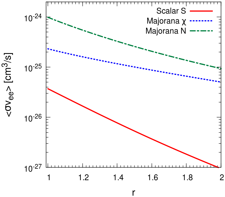
Figure I: Annihilation cross sections into a SM fermion pair as a function of $r=M_{med}/M_{DM}$ (thermal averages and in the chiral limit). The cross sections are given for unit couplings and for $M_{DM}=100$ GeV.

III Spectral energy density: internal Bremsstrahlung

In this section we discuss the contribution of so-called internal Bremsstrahlung to the spectral energy density of gamma rays. This has been discussed extensively in the literature, so we just recap the salient features. Bremsstrahlung is of interest for two reasons. First, the annihilation cross section in a s-wave through Bremsstrahlung is no longer mass suppressed. For one thing, there is no obstruction from conservation of angular momentum, but there is more to it. Although the argument is somewhat gauge-dependent, this result may be traced to emission of a gamma ray from the virtual massive charged particle in the t- and u-channels, or so-called virtual internal Bremsstrahlung (see e.g. Bringmann et al. (2008)). This implies that the Bremsstrahlung, a 3-body final state process, may be more important than the 2-body tree level process, despite the suppression of the former by a factor ${\cal O}(\alpha/\pi)$. This is typically the case for annihilation in light fermions or equivalently heavy dark matter $M_{DM}\gg m_{f}$, and when the velocity is non-relativistic, like at the galactic center ($v\sim 10^{-3}$). Second, emission from the virtual mediator, depending on the ratio $r=M_{med}/M_{DM}$, may have a sharp spectral feature, possibly mimicking a monochromatic gamma ray line.

For reference, we give here the expressions of the 3-body annihilation cross section for the 3 scenarios. Defining

$$vd\sigma_{2\rightarrow 3} = \frac{|{\cal M}|^{2}}{128\pi^{3}}dxdy$$ (13)

where $v={\sqrt{{k_{1}\cdot k_{2}}-m_{1}m_{2}}}/{E_{1}E_{2}}$ refers to the relative velocity of the $S$ particles and $x,y$ are the reduced energy parameters $x=2E_{\gamma}/\sqrt{s}$ and $y=2E_{f}/\sqrt{s}$, with $s$ the Mandelstam variable corresponding to the center-of-mass energy squared, we have:

III.0.1 Scenario $1$: $\chi$ DM candidate Bergstrom (1989)

$${1\over 4}\sum_{\rm spin}|{\cal M}_{\chi}|^{2}=\frac{4\,\pi\,\alpha\,y_{\chi}^{4}}{M_{\chi}^{2}}\,\frac{4(1-y)(2+2x^{2}+2x(y-2)-2y+y^{2})}{(1-r_{\chi}^{2}-2x)^{2}(3+r_{\chi}^{2}-2x-2y)^{2}}$$ (14)

III.0.2 Scenario $2$: $N$ DM candidate Barger et al. (2012)

$${1\over 4}\sum_{\rm spin}|{\cal M}_{N}|^{2}=\frac{\,\pi\,\alpha\,g_{N}^{4}}{M_{N}^{2}}\left(2+{1\over r_{N}^{2}}\right)^{2}\,\frac{4(1-y)(2+2x^{2}+2x(y-2)-2y+y^{2})}{(1-r_{N}^{2}-2x)^{2}(3+r_{N}^{2}-2x-2y)^{2}}$$ (15)

III.0.3 Scenario $3$: $S$ DM candidate Barger et al. (2012); Toma (2013); Giacchino et al. (2013)

$$|{\cal M}_{S}|^{2}=\frac{32\pi\,\alpha\,y_{S}^{4}}{M_{S}^{2}}\,\frac{4(1-y)(2+2x^{2}+2x(y-2)-2y+y^{2})}{(1-r_{S}^{2}-2x)^{2}(3+r_{S}^{2}-2x-2y)^{2}}$$ (16)

The acute reader will have noticed that, for fixed $r_{\chi,N,S}$, the dependence of the Bremsstrahlung cross sections into gamma rays is precisely the same in Eqs. (14,15,16), which implies that all three scenarios have the same spectral signature Barger et al. (2012). Notice that we have already checked this dependence for both scenarios $1$ and $3$ in Giacchino et al. (2013). The Bremsstrahlung cross section in the scalar case was also re-derived in Toma (2013) and previously obtained in the large mediator mass regime in Boehm and Uwer (2006).

An argument to explain this conclusion has been advanced in Barger et al. (2012) based on effective operators. First there should be no distinction between scenarios $1$ and $2$ since they have the same initial and final states. As above, the bi-linear operator corresponding to the initial states is $\bar{\chi}\gamma_{5}\chi$. Then they have shown that Bremsstrahlung corresponds to the effective operator

$${\cal O}_{\chi}\sim\bar{\chi}\gamma_{5}\chi\,\left(\partial_{\mu}\bar{\psi}_{R}\gamma_{\nu}\psi_{R}+\bar{\psi}_{R}\gamma_{\nu}\partial_{\mu}\psi_{R}\right)\tilde{F}^{\mu\nu}\,,$$ (17)

where $\tilde{F}^{\mu\nu}$ is the dual of $F^{\mu\nu}$. In scenario $3$, the initial state corresponds to $S^{2}$ and the effective coupling is given by

$${\cal O}_{S}\sim S^{2}\,\left(\partial_{\mu}\bar{\psi}_{R}\gamma_{\nu}\psi_{R}+\bar{\psi}_{R}\gamma_{\nu}\partial_{\mu}\psi_{R}\right)F^{\mu\nu}$$ (18)

The only difference amounts to exchanging the role of the $\vec{E}$ and the $\vec{B}$ of the photon and so the spectra are the same (up to normalization). This argument is essentially based on a rephrasing of the exact result in terms of effective operators, and thus is not per se an explanation, but it may complemented as follows. Notice that the effective couplings correspond to respectively a dimension 9 and 8 operator, but there are other, a priori independent, operators. Incidentally a classification of all dimension 8 operators contributing to photon Bremsstrahlung for both Majorana and scalar DM has been given in De Simone et al. (2013): for Majorana DM there are 5 operators, out of which 3 are CP even, while in the scalar case, there are 7 operators, with 4 being CP even. Remarkably, while these operators lead to different spectra for the emission of $W$ and $Z$, the spectra for emission of gamma rays are precisely the same (see Eqs. (3.8)-(3.10) and Eqs. (3.24)-(3.27) in De Simone et al. (2013)). Moreover, it can be easily checked that they have the same $x$ and $y$ dependence as the numerator of Eqs. (14), (15) and (16) (after some obvious change of variables). This, in passing, means that the dimension 9 operator for Majorana DM of Eq. (17) must be equivalent to (a combination of) the dimension 8 operators studied in De Simone et al. (2013). While the $r$ dependence of the denominator in Eqs. (14)-(16) can not be obtained from an effective approach, it may be easily inferred from the propagators of the intermediate particles. Hence the effective operator argument that Bremsstrahlung from scalar and Majorana DM should have the same spectra is actually robust.

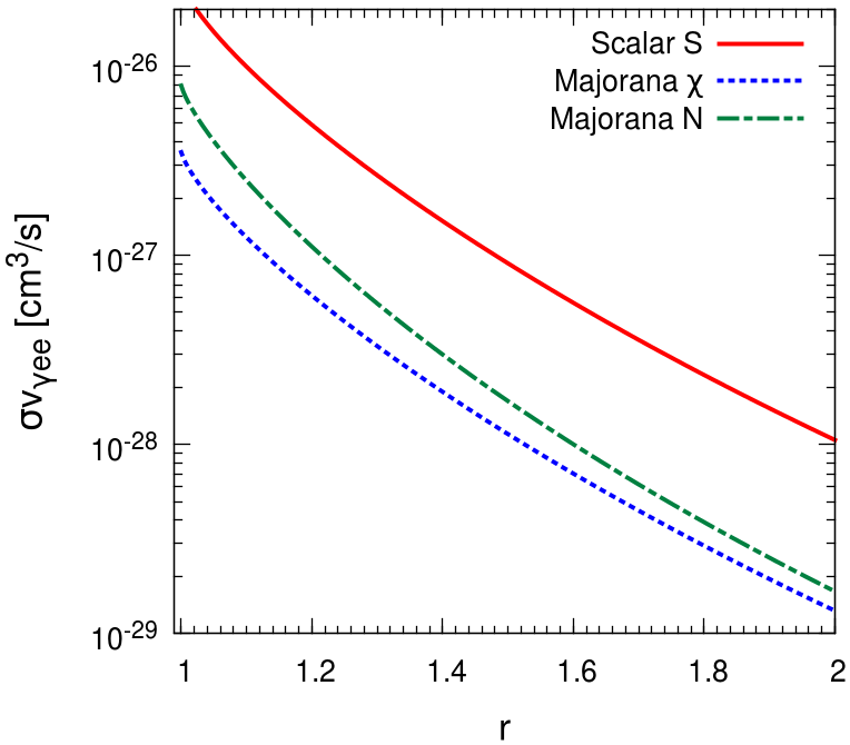
Figure II: Total 3-body cross sections (gamma ray Bremsstrahlung emision). Same conventions as in Fig. I.

Now it remains that the normalizations of the spectra are distinct, or at least they are for the scalar, for scenarios $1$ and $2$ are quite similar. For equal $M_{DM}$, couplings and $r$, the amplitude in the gauge case is larger by a factor of

$${1\over 2}\left(2+{M_{N}^{2}\over M_{W^{\prime}}^{2}}\right)\sim 1$$

where the first term is from the 2 transverse polarization modes and the second term from the longitudinal one. As emphasized in Toma (2013); Giacchino et al. (2013), all things being taken to be the same (i.e. DM and mediator masses and the couplings), the 3-body cross section is larger by a factor of 8 in scenario $3$ compared to scenario $1$. This, together with the relative suppression of the 2-body cross section leads to an enhanced gamma ray feature in the scalar case compare to the Majorana cases.

The intermediate conclusion is that scenarios $1$ and $2$ are essentially identical. They share the same spectra, with quasi the same parametric dependence in the couplings and mass of DM and of the mediator of the normalization of the 2 and 3-body processes. The scalar case is distinct, in the sense that if the relic abundance is thermal and is fixed by the 2-body annihilation process, then the signal is stronger for the scalar case (by a factor which may be as large as 2 orders of magnitude) Toma (2013); Giacchino et al. (2013). If we relax the latter constraint (for instance if the abundance is fixed by another process), then the 3 scenarios become indistinguishable. It is thus of interest to check whether other spectral features may help to lift this degeneracy. The spectrum of gamma rays from say, $\pi_{0}$, being featureless we focus on gamma ray lines. In Giacchino et al. (2013) we have tentatively included the features from annihilation into two monochromatic gamma rays. However the one-loop cross sections, in particular that relevant for scenario $3$, reported in the literature has some peculiarities. We have thus felt compelled to reanalyze this problem. Our results are presented in the next section.

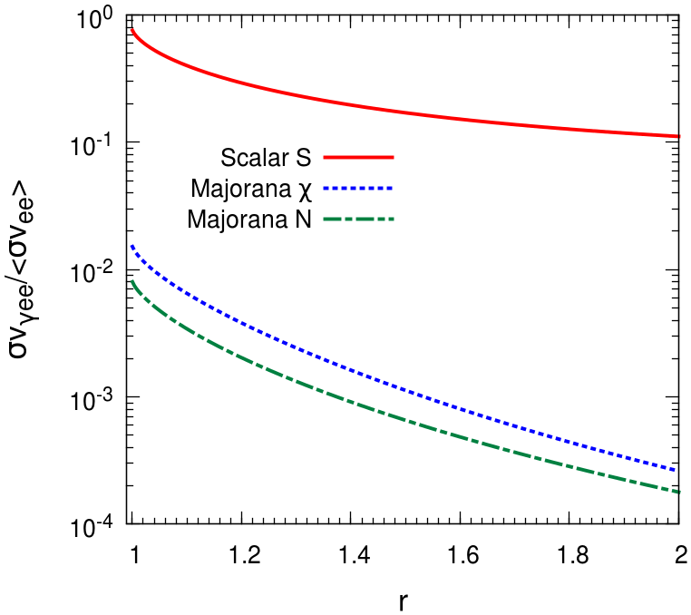
Figure III: Ratios of the 3-body (gamma ray Bremsstrahlung emision) to 2-body annihilation cross sections. The 2-body cross section is thermally averaged over velocities at the time of freeze-out, relevant to determine the relic abundance of DM.

IV SPECTRAL ENERGY DENSITY: GAMMA RAY LINES

We consider the annihilation of non-relativistic DM into two on-shell gamma rays,

$$DM(p_{1})+DM(p_{2})\rightarrow\gamma(\epsilon_{1},k_{1})+\gamma(\epsilon_{2},k_{2})$$

with $p_{1,2}$ and $k_{1,2}$ the momenta, $\epsilon_{1,2}$ the polarization vectors, $p_{1}+p_{2}=k_{1}+k_{2}$, and $\epsilon_{1}\cdot k_{1}=\epsilon_{2}\cdot k_{2}=0$.

In the 3 scenarios we consider the amplitude for this process is represented by a sum of box Feynman diagrams. Although the individual diagrams may be infinite, the total amplitudes are finite and are moreover non-vanishing in the s-wave. These features allow substantial simplifications in the calculation of the Feynman diagrams. In particular we can calculate the amplitude in the limit $p_{1}=p_{2}=(M_{DM},\vec{0})$. In this limit, Gram determinants built on the external momenta or their relevant linear combinations may be vanishing. For instance

$$\left|\begin{array}[]{ccc}p_{1}^{2}&p_{1}\cdot p_{2}&p_{1}\cdot k_{1}\\ p_{1}\cdot p_{2}&p_{2}^{2}&p_{2}\cdot k_{1}\\ p_{1}\cdot k_{1}&p_{2}\cdot k_{1}&k_{1}\cdot k_{1}\\ \end{array}\right|=0$$

The standard Passarino-Veltman reduction of tensorial loop integrals breaks down when Gram determinant are zero Passarino and Veltman (1979). This is in particular an issue for automated tools like FormCalc and is also a source of numerical instabilities in LoopTools Hahn and Perez-Victoria (1999). Fortunately, by the very same token, one may use the degeneracy between the momenta to express 4-point integrals in terms of 3-point integrals, and also some 3-points integrals in terms of 2-points integrals Stuart (1988) (see also Bergstrom and Ullio (1997); Bertone et al. (2009)). In particular this implies that no 4-points loop integrals appear in the final expression of the amplitude, which may be expressed in terms of finite, 3-points loop integrals that are much easier to handle, and in particular may be given in terms of rather simple analytic functions. As in the previous section, we discuss the 3 scenarios separately.

IV.0.1 Scenario $1$: $\chi\chi\rightarrow\gamma\gamma$

This process has been calculated several times, starting from the seminal works of Bergstrom and Snellman (1988); Rudaz (1989); Bergstrom (1989) in the context of supersymmetry. As is well known, in the limit $M_{\tilde{E}}\gg M_{\chi}$, the amplitude for $\chi\chi\rightarrow\gamma\gamma$ may be related to the chiral anomaly. A remarkable consequence is that the amplitude does not vanish in the chiral limit, $m_{f}\rightarrow 0$.

For our own sake and to check our procedures, we have redone the calculation of this amplitude in the non-relativistic limit, $v_{\chi}\rightarrow 0$, albeit with the help of FeynCalc Mertig et al. (1991). To do so we have used the trick of Bergstrom and Ullio (1997) which consists of projecting the initial $\chi$ pair into a s-wave state, using

$${\cal O}=-{M_{\chi}\over\sqrt{2}}\gamma_{5}\left(1-\gamma^{0}\right)\,.$$

In the chiral limit the amplitude involves a single 3-points scalar loop integral. For reference, we give its expression following the standard nomenclature of 3-point loop integrals (the $C_{0}$ functions of Passarino and Veltman) and then explicitly in terms of analytic functions. We have found

$$\langle\sigma v\rangle_{\gamma\gamma}^{\chi}=\frac{y_{\chi}^{4}\alpha^{2}M_{\chi}^{2}}{64\pi^{3}}\left|C_{0}\left(-M_{\chi}^{2},M_{\chi}^{2},0,r_{\chi}^{2}M_{\chi}^{2},0,r_{\chi}^{2}M_{\chi}^{2}\right)\right|^{2}\,.$$ (19)

Using

$$C_{0}(-M^{2},M^{2},0,r^{2}M^{2},0,r^{2}M^{2}) = {-1\over 2M^{2}}\int_{0}^{1}{dx\over x}\log\left(\left|{-x^{2}+(1-r^{2})x+r^{2}\over x^{2}-(1+r^{2})x+r^{2}}\right|\right)$$ (20)

$$= {-1\over 2M^{2}}\left(Li_{2}\left({1\over r^{2}}\right)-Li_{2}\left({-1\over r^{2}}\right)\right)$$ (21)

we are in complete agreement with previous results and in particular with Bergstrom and Ullio (1997); Bern et al. (1997) (we have also calculated the amplitude for the case $m_{f}\neq 0$ - the result may be read from Bergstrom and Ullio (1997)). Of interest for us will be the following limits,

$$\langle\sigma v\rangle_{\gamma\gamma}^{\chi} = \frac{y_{\chi}^{4}\alpha^{2}\pi}{64^{2}M_{\chi}^{2}}\quad\mbox{for }r_{\chi}=1\quad\mbox{and }\quad\langle\sigma v\rangle_{\gamma\gamma}^{\chi}\approx\frac{y_{\chi}^{4}\alpha^{2}}{64\pi^{3}}{M_{\chi}^{2}\over M_{\tilde{E}}^{4}}\quad\mbox{for }r_{\chi}\gg 1$$ (22)

IV.0.2 Scenario $2$: $NN\rightarrow\gamma\gamma$

For this process we refer to the work of Bergstrom and Ullio (1997) in which a related amplitude has been calculated. Specifically, the process considered there is the annihilation of two neutralinos into two photons through a chargino and SM $W^{\pm}$ gauge boson loops. Making simple adjustments in the couplings and the particle content, and taking into account the coupling to nonphysical Goldstone modes (as alluded to above, the calculation of Bergstrom and Ullio (1997) has been done in a ’t Hooft-Feynman non-linear $R_{\xi}$ gauge), we get

$$\langle\sigma v\rangle_{\gamma\gamma}^{N} = \frac{g_{N}^{4}\alpha^{2}M_{N}^{2}}{64\pi^{3}}\left|4C_{0}(4M_{N}^{2},0,0,r_{N}^{2}M_{N}^{2},r_{N}^{2}M_{N}^{2},r_{N}^{2}M_{N}^{2})\right.$$ (23)

$$-\left.\left(2+\frac{1}{r_{N}^{2}}\right)C_{0}(-M_{N}^{2},M_{N}^{2},0,r_{N}^{2}M_{N}^{2},0,r_{N}^{2}M_{N}^{2})\right|^{2}$$

with

$$C_{0}(4M^{2},0,0,r^{2}M^{2},r^{2}M^{2},r^{2}M^{2}) = {1\over 4M^{2}}\int_{0}^{1}\frac{dx}{x}\log\left(\left|4\frac{x^{2}}{r^{2}}-4\frac{x}{r^{2}}-1\right|\right)$$ (24)

$$= {-1\over 2M^{2}}\left(\arctan{1\over\sqrt{r^{2}-1}}\right)^{2}$$ (25)

where the last equality holds for $r\geq 1$ and the other $C_{0}$ are as defined in Eq. (20). The limiting behaviours are now given by

$$\langle\sigma v\rangle_{\gamma\gamma}^{N} = \frac{g_{N}^{4}\alpha^{2}\pi}{64^{2}M_{N}^{2}}\frac{25}{4}\quad\mbox{for }r_{N}=1\quad\mbox{and }\quad\langle\sigma v\rangle_{\gamma\gamma}^{N}\approx\frac{g_{N}^{4}\alpha^{2}}{64\pi^{3}}{M_{N}^{2}\over M_{W^{\prime}}^{4}}\quad\mbox{for }r_{N}\gg 1\,.$$ (26)

As an independent check of this result, we have verified that we can recover the cross-sections derived many years ago by Crewther et al Crewther et al. (1982), for the annihilation of SM neutrinos into two photons, in a regime corresponding to our limit $r_{N}\gg 1$ in Eq. (26) (see Appendix A).

IV.0.3 Scenario $3$: $SS\rightarrow\gamma\gamma$

For this case we have redone the full one-loop calculation, including finite SM fermion mass $m_{f}\neq 0$ contributions. The full expression is given in the Appendix B. Here we just give the expression in the chiral limit, as for the other two scenarios.

To derive the amplitude, we have essentially followed the path of Bertone et al. (2009). We made use of FeynCalc and calculated amplitude and cross section for S particles at rest ($v_{S}=0$). This amounts to evaluate a combination of one-loop 4-points tensor integrals. Since the Gram determinant is zero for DM particles at rest, a straightforward application of Passarino-Veltman reduction does not work, so instead we used the approach of Stuart (1988) to express directly the 4-points loop integrals as a linear combination of 3-points scalar integrals.

Writing

$$\langle\sigma v\rangle_{\gamma\gamma}=\frac{2\,y_{S}^{4}\alpha^{2}}{64\pi^{3}M_{S}^{2}}|{\cal A}|^{2}$$ (27)

at an intermediate step we got the following expression (for $m_{f}=0$)

$${\cal A} = 2+\frac{2}{(1-r_{S}^{2})}B_{0}\left(M_{S}^{2},0,r_{S}^{2}M_{S}^{2}\right)-B_{0}\left(4M_{S}^{2},0,0\right)-\frac{1+r_{S}^{2}}{1-r_{S}^{2}}B_{0}\left(4M_{S}^{2},r^{2}M_{S}^{2},r_{S}^{2}M_{S}^{2}\right)$$

$$+M_{S}^{2}\left(-(1+r_{S}^{2})\left(C_{0}\left(M_{S}^{2},M_{S}^{2},4M_{S}^{2},0,r_{S}^{2}M_{S}^{2},0\right)+C_{0}\left(M_{S}^{2},M_{S}^{2},4M_{S}^{2},r^{2}M_{S}^{2},0,r_{S}^{2}M_{S}^{2}\right)\right)\right.$$

$$\left.-2C_{0}\left(-M_{S}^{2},M_{S}^{2},0,r_{S}^{2}M_{S}^{2},0,r_{S}^{2}M_{S}^{2}\right)+4r_{S}^{2}C_{0}\left(4M_{S}^{2},0,0,r_{S}^{2}M_{S}^{2},r_{S}^{2}M_{S}^{2},r_{S}^{2}M_{S}^{2}\right)\right)\,.$$

Despite the presence of divergent 2-point integrals, this expression is finite. Actually it may be simplified using the fact that some 3-point scalars integral, whose momentum arguments have a vanishing Gram determinant, may be reduced further

$$C_{0}\left(M_{S}^{2},M_{S}^{2},4M_{S}^{2},M_{E}^{2},0,M_{E}^{2}\right) = \frac{B_{0}\left(M_{S}^{2},0,M_{E}^{2}\right)-B_{0}\left(4M_{S}^{2},M_{E}^{2},M_{E}^{2}\right)}{-M_{E}^{2}+M_{S}^{2}}$$ (29)

$$C_{0}\left(M_{S}^{2},M_{S}^{2},4M_{S}^{2},0,M_{E}^{2},0\right) = \frac{B_{0}\left(M_{S}^{2},0,M_{E}^{2}\right)-B_{0}\left(4M_{S}^{2},0,0\right)}{M_{E}^{2}+M_{S}^{2}}$$ (30)

Using this substitution, we get the following simple expression

$${\cal A}=2-2M_{S}^{2}C_{0}(-M_{S}^{2},M_{S}^{2},0,r_{S}^{2}M_{S}^{2},0,r_{S}^{2}M_{S}^{2})+4r_{S}^{2}M_{S}^{2}C_{0}(4Ms^{2},0,0,r_{S}^{2}M_{S}^{2},r_{S}^{2}M_{S}^{2},r_{S}^{2}M_{S}^{2})\,.$$ (31)

where the two 3-points loop integrals are those given in Eqs. (20,24).

Finally for $r_{S}=1$ and $r_{S}\gg 1$, we have respectively

$$\langle\sigma v\rangle_{\gamma\gamma}^{S} = \frac{y_{S}^{4}\alpha^{2}}{8\pi^{3}M_{S}^{2}}\left(1-\frac{\pi^{2}}{8}\right)^{2}\quad\quad\mbox{and }\quad\langle\sigma v\rangle_{\gamma\gamma}^{S}\approx\frac{y_{S}^{4}\alpha^{2}}{18\pi^{3}M_{S}^{2}r^{4}}\hskip 28.45274pt$$ (32)

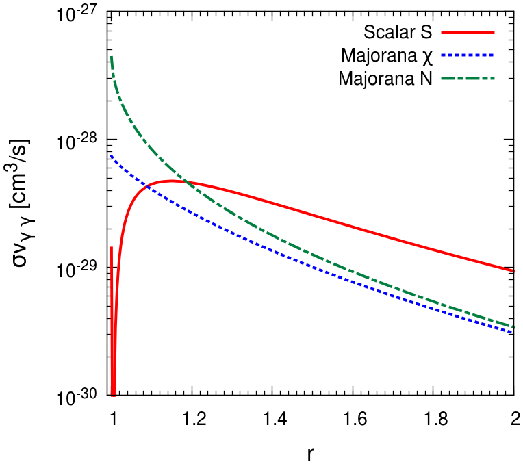
Figure IV: Annihilation into 2 photons. Same conventions as in Fig.I.

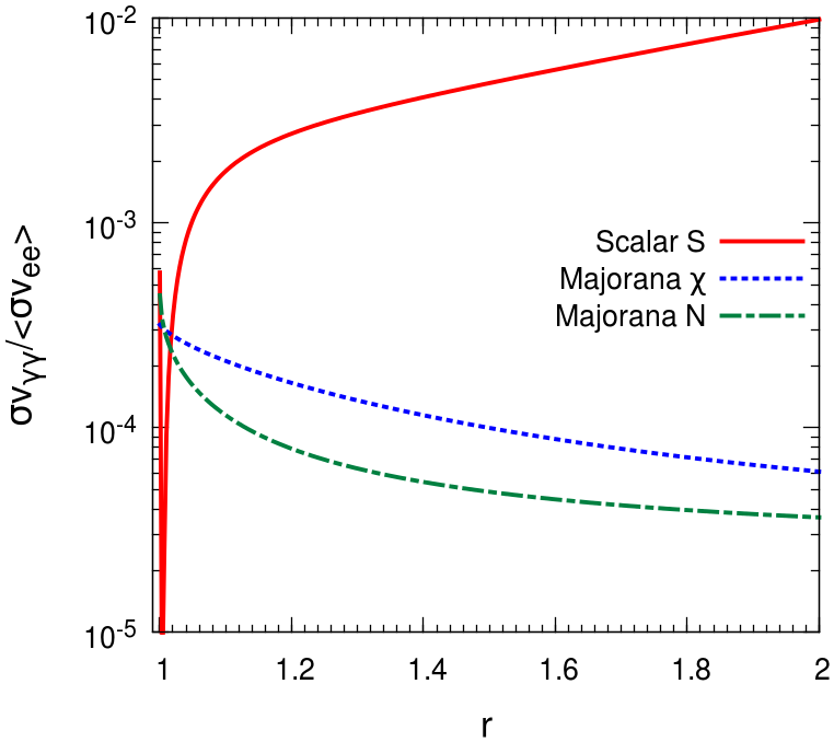
Figure V: Ratios of the cross sections into 2 photons to the 2-body annihilation into a fermion pair.

V Discussion of results

In this section we compare the salient features of the 3 scenarios considered in the previous section. The thermally averaged 2-body annihilations cross sections into two fermions at the time of freeze-out (i.e. for averaged velocities taken as in Eq. (12)) in the chiral limit are shown in Fig. I. For convenience we have normalized all the couplings to 1 and we took $M_{DM}=$ 100 GeV. This figure shows that the cross section in the scalar DM scenario (scenario $3$) is parametrically smaller than that of scenarios with Majorana DM (scenarios 1 and 2): while scenarios 1 and 2 (for $\chi$ and $N$ DM) share the same asymptotic behaviour for large $r$, the thermally averaged cross section in scenario 3 (for $S$ DM) for, say $r=2$, is suppressed by almost 2 orders of magnitude. This result is due to a combination of the d-wave dependence of the cross section and of a distinct dependence on $r$, see Eqs. (8), (7) and (II.3). If the relic abundance is fixed by the 2-body process, a larger coupling is thus required for the $S$ than for the $\chi$ or $N$ scenarios Toma (2013); Giacchino et al. (2013).

In Fig. II, we give the 3-body annihilation cross section (for photon Bremsstrahlung emission) again for unit couplings and $M_{DM}=100$ GeV. The $r$-dependences are very similar, but the signal from $S$ is comparatively larger compared to the $\chi$ and $N$ scenarios, respectively by a factor $8$ and $8/(1+1/2r^{2})^{2}$. This, combined with the previous feature, implies that the Bremsstrahlung is potentially much stronger in the $S$ scenario, although the spectra are the same Toma (2013); Giacchino et al. (2013). This is illustrated in Fig. III which shows the ratio of the 3-body to 2-body cross sections (note that this ratio is independent of the couplings and of the mass of the DM candidate). If the 2-body annihilation into two fermions is the one driving the relic abundance in the early universe, the Bremsstrahlung spectral feature is expected to be much stronger in the scalar DM scenario ($\langle\sigma v\rangle_{\gamma ll}$ is almost 3 orders of magnitude larger than for Majorana DM for $r\sim 2$).

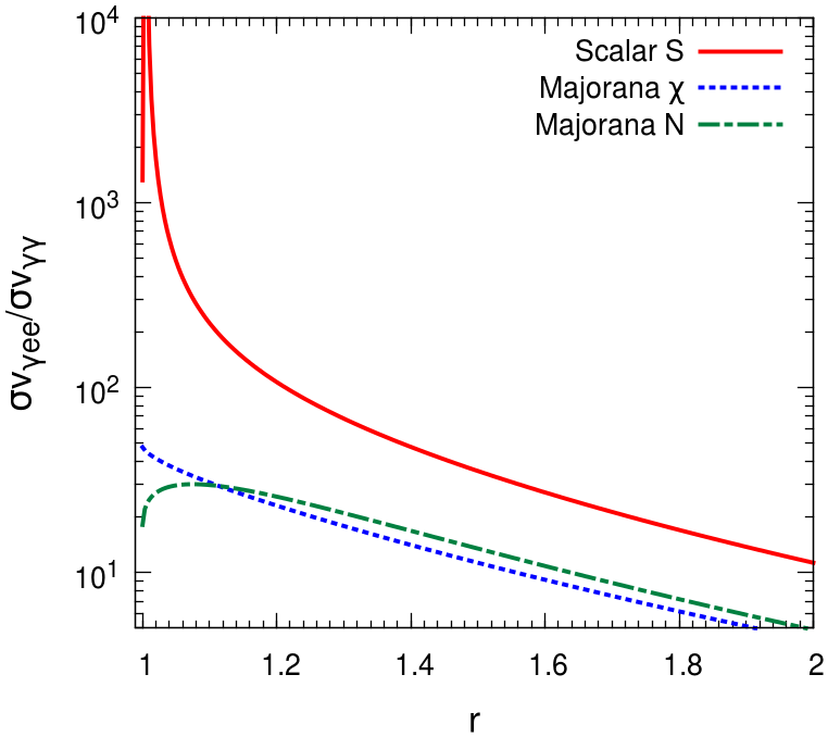
Figure VI: Ratios of the Bremsstrahlung to 2 photons cross sections.

Turning to the annihilation into monochromatic gamma rays, we compare the three cross sections in Fig. IV. The dependence in the $\chi$ scenario is well-known, and has been reported many times in the literature. In particular, it may be related to the chiral anomaly, which implies that the cross section is non-vanishing even in the chiral limit Rudaz (1989); Bergstrom (1989). Since the initial and final states are the same in scenarios $1$ and $2$, one may expect a similar behaviour, which is confirmed by the calculations and is illustrated in Fig. IV. Although this result is implicit in the literature (we derive the $N$ cross section from the results on the neutralino discussed in Bergstrom and Ullio (1997)), we are not aware of an explicit discussion in the framework of simpler models, like that of Khalil et al. (2009); Ma (2009). At any rate, the cross section is that given in Eq. (23). It is slightly larger than in the $\chi$ scenario for $r$ close to 1 (by a factor of $25/4$ at $r=1$), but asymptots to the same result at large $r$. The large $r$ behaviour is also in agreement with the result of Crewther et al for the annihilation of Dirac neutrinos into two photons Crewther et al. (1982). Incidentally, the latter result has been derived making use of the chiral anomaly, as in the early derivation of the cross section in the $\chi$ scenario.

The behaviour of the cross section in scenario $3$ is more puzzling. Having done the calculation using different approaches, and also having obtained the same results as those reported in Ibarra et al. (2014), we are confident that the expression is correct. In particular it is finite at $r=1$, albeit with a strange value compared to the Majorana cases. The large $r$ behaviour is also completely mundane, having the same dependence in $r$ as in scenarios $1$ and $2$. It shows however peculiar feature, since it has a maximum around $r=1.15$ and then a dip, with a zero near $r=0$. The origin of this destructive interference is unclear, at least to us, although it may be traced to amplitudes that correspond to Feynman diagrams with a distinct number of heavy fermion propagators. It may be of academic interest to investigate this phenomenon further, which may perhaps be related to the distinct property of the tree level annihilation cross section into fermion pairs in the $S$ scenario compared to the Majorana cases. Another, perhaps not unrelated question is whether the annihilation cross section of $S$ into two photons may be derived from the trace anomaly.

This being said, we see that the $S$ cross section is larger by a factor of $32/9\approx 3.5$ than in the Majorana DM scenarios, which have the same asymptotic behaviour. The annihilation of a scalar may thus also lead to a relatively stronger signal into monochromatic photons. This is shown in Fig. V, which displays the ratio of the cross section into 2 gamma rays to that into a fermion pair. The rise as a function of $r$ of the signal in the $S$ case is due to the fact that the 2-body cross section into fermion pairs scales like $r^{-6}$, see Eq. (II.3), while the annihilation into 2 photons is $\propto r^{-4}$, see Eq. (32). On the contrary the ratios asymptote to a small constant, ${\cal O}(10^{-5})$, for the Majorana scenarios.

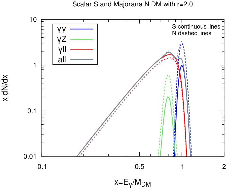
Figure VII: Comparison of normalized photon spectra for scenarios 2 and 3 for $M_{DM}=100$ GeV.

For completeness we also give in Fig. VI the ratio of 3-body annihilation cross section (photon Bremsstrahlung emission) to the one into two photons. The Bremsstrahlung signal becomes relatively less prominent for large $r$, as the cross sections drop like $r^{-6}$, but we see it is more dominant in the scalar than in the Majorana scenarios. Hence both signals are stronger for the scalar. The relative importance of the $\gamma\gamma$ signal compared to the $\gamma ee$ one is however comparatively smaller in the scalar case than in the Majorana DM cases. This may be seen directly in the photon spectra of Fig. VII where we compare scenario 2 and 3 ($N$ and $S$) for $r=2$; scenario 1 ($\chi$) would have essentially the same signature as scenario 2. The quantity $xdN/dx=E_{\gamma}/\sigma v_{\gamma}d\sigma v_{\gamma i}/dE_{\gamma}$, with $i=\gamma,ee$ and $\sigma v_{\gamma}=\sum_{i}\sigma v_{\gamma i}$, denotes the normalized photon spectrum multiplied by the photon energy. We see that for $r=2$ the dominant Bremsstrahlung feature gets an extra contribution from the $\gamma\gamma$ and $\gamma Z$ lines. Notice that we have assumed an energy resolution of $\Delta E/E=0.1$, and that, although we did not explicitly derived $\langle\sigma v\rangle_{\gamma Z}$ here, we follow the same procedure as in Giacchino et al. (2013) to estimate the $\gamma Z$ contribution. We refer to Toma (2013); Giacchino et al. (2013) for some discussion of scenarios $1$ and $3$. Clearly scenario $2$ should give a phenomenology similar to that of the $\chi$ Majorana. Here we just provide a few benchmark values (see Table 1).

	Scenario $1$ ($\chi$)		Scenario 2 ($N$)		Scenario 3 ($S$)
	$r=$1.2	$r=2$	$r=1.2$	$r=2$	$r=1.2$	$r=2$
$\langle\sigma v\rangle_{\gamma ll}$	$6.1\,10^{-28}$	$1.3\,10^{-29}$	$1.1\,10^{-27}$	$1.7\,10^{-29}$	$4.9\,10^{-27}$	$1.1\,10^{-28}$
$\langle\sigma v\rangle_{\gamma\gamma}$	$2.9\,10^{-29}$	$3.1\,10^{-30}$	$4.3\,10^{-29}$	$3.4\,10^{-30}$	$4.6\,10^{-29}$	$9.4\,10^{-30}$

Table 1: Cross sections in units of cm³/s for $M_{DM}=100$ GeV and unit couplings

VI Conclusions

In this work we have complemented the work of Barger et al, in which 3 simple scenarios of DM with Bremsstrahlung of photons are discussed. It also complements the phenomenological studies initiated in Toma (2013) and Giacchino et al. (2013) in which it has been shown that a real scalar DM candidate $S$ interacting with light SM fermions could give a strong Bremsstrahlung signal. Specifically we have considered the radiative annihilation of three DM candidates into two photons. This lead us to re-calculate the amplitude for $SS\rightarrow\gamma\gamma$. Our result differs from expressions that may be found in the literature, but the discrepancy is minor, being likely due to a misprint, which however is difficult to spot without actually doing the full calculation. Hence we believe that it was useful to provide an independent check of the expression for $SS\rightarrow\gamma\gamma$. We have compared the result to those expected in the case of a Majorana DM, interacting with SM fermions either through a heavy charged scalar particle (scenario 1) or through a charged gauge boson (scenario 2). The main outcome, which complement the conclusions drawn in Toma (2013) and Giacchino et al. (2013), is that radiative processes are significantly more relevant for the scenario with scalar DM than for the Majorana cases. These results from a combination of factors. First the fact that the annihilation cross section into fermion pairs is d-wave suppressed in the chiral limit in the scalar DM case, and second, the fact that the radiative cross section are parametrically larger. These results may be directly inferred from the analytical expressions given in the body of the paper, and from a glance at the figures.

Appendix A From $\bar{N}N\rightarrow\gamma\gamma$ to $\bar{\nu}\nu\rightarrow\gamma\gamma$

In this appendix we compare the cross section for annihilation in two photons in scenario 2 to the annihilation of Dirac SM neutrinos calculated by Crewther et al Crewther et al. (1982). In Crewther et al. (1982), they effectively made use of the following Lagrangian:

$${\cal L}_{eff}=\frac{G_{F}}{2\sqrt{2}}\bar{\nu}(1-\gamma_{5})\nu\,\bar{e}\gamma_{\mu}(1+4s_{W}^{2}-\gamma_{5})e\,.$$ (33)

They indeed show that all other possible contributions are negligible. This has to be compared to the corresponding effective Lagrangian resulting from our Eq. (3):

$${\cal L}_{eff}=\frac{g_{N}^{2}}{8M_{W^{\prime}}^{2}}\bar{N}(1+\gamma_{5})N\,\bar{e}\gamma_{\mu}(1+\gamma_{5})e\,.$$ (34)

The main differences come from the overall factor: $\frac{g_{N}^{2}}{8M_{W^{\prime}}^{2}}\rightarrow\frac{G_{F}}{2\sqrt{2}}$ and the vector contributions to the neutrinos $N,\nu$ and the electron currents. It can be shown that none of the latter contributions to the $N,\nu,e$ currents are relevant for the final result. In addition, Crewther et al assumed that the SM neutrinos $\nu$ were of Dirac type while in our case $N$ are Majorana neutrinos. This implies that our final cross-section should be divided by a factor of 4 due to the fact that two directions of the fermionic current flow are possible for the Majorana particles to describe the same interaction (see also e.g. Rudaz (1989)). Departing from (26) in the limit $r_{N}\gg 1$, we obtain for $M_{N}\rightarrow m_{\nu}$:

$$\langle\sigma v\rangle_{\gamma\gamma}^{\nu}=\frac{1}{4}\frac{\alpha^{2}G_{F}^{2}m_{\nu}^{2}}{8\pi^{3}}\,,$$ (35)

where the $\frac{1}{4}$ factor comes from the Majorana to Dirac neutrino change. This equations has to be compared to equation (2.30) in Crewther et al. (1982) where their $\sigma c$ corresponds $\sigma\sqrt{1-4m_{\nu}^{2}/s}=\langle\sigma v\rangle_{\gamma\gamma}^{\nu}/2$ or equivalently to the cross-section times the velocity of one dark matter particle. One can check that our Eq. (35) perfectly match their Eqs. (2.28)-(2.30), realizing that in the chiral limit, their function $I(m_{e}^{2}/s)\rightarrow 12m_{e}^{2}/s$ and allows to cancel the $m_{e}$ insertions in their Eq. (2.28).

Appendix B Full expression of $\langle\sigma v\rangle_{\gamma\gamma}^{S}$

If $m_{l}\neq 0$ the expression of the amplitude for $SS\rightarrow\gamma\gamma$ (s-wave contribution) in Eq. (31) should be replaced by

$${\cal A} = 2+\left[4\,\frac{m_{l}^{2}(m_{l}^{2}-M_{S}^{2})C_{0}(4M_{S}^{2},0,0,m_{l}^{2},m_{l}^{2},m_{l}^{2})}{m_{l}^{2}-M_{S}^{2}(r_{S}^{2}+1)}\right.$$ (36)

$$\hskip 28.45274pt+2m_{l}^{2}M_{S}^{2}\,\frac{\left(m_{l}^{2}(-m_{l}^{2}+2M_{S}^{2})+M_{S}^{4}(r_{S}^{2}-1)\right)C_{0}(-M_{S}^{2},M_{S}^{2},0,m_{l}^{2},r_{S}^{2}M_{S}^{2},m_{l}^{2})}{(m_{l}^{2}-r_{S}^{2}M_{S}^{2})(m_{l}^{2}-M_{S}^{2}(r_{S}^{2}+1))(m_{l}^{2}-M_{S}^{2}(r_{S}^{2}-1))}$$

$$\hskip 28.45274pt+(m_{l}\leftrightarrow r_{S}M_{S})\bigg{]}$$

Notice that we have made use of (30) to obtain (36).

Note Added

During the completion of this work we learned about the analysis of Ibarra et al. (2014) on the scalar dark matter scenario that includes a gamma-ray spectral feature analysis. Their results agree with ours in the aspects where our analysis overlap.