Diffusion of two brands in competition: cross-brand effect

Abstract

We study the equilibrium points of a system of equations corresponding to a Bass based model that describes the diffusion of two brands in competition. To increase the understanding of the effects of the cross-brand parameters, we perform a sensitivity analysis. Finally, we show a comparison with an agent-based model inspired in the Potts model. Conclusions include that both models give the same diffusion curves only when the cross coeficients are not null.

1
Introduction

It is of present interest, from an economic point of view, to fully understand the processes and drivers behind the diffusion of innovations. The existence of many recent papers reviewing this subject, such as [1], [2] and [3] are an example of its relevance. A pioneer work is the well-known Bass model [4] which describes the curves of adoption for many durable goods with great precision.

Keeping in mind the success of the Bass model in the description of the diffusion process of many new products, it is natural to extend the formalism to describe the adoption curves of two brands which are launched simultaneously and dispute the same market. This possibility has been previously investigated, as we can see in [5] and [3].

We have, within the Bass formalism, two coupled differential equations. The simplest coupling is the one associated to the competition between two brands within a common market. However, as in [6], a cross-brand effect can be introduced that takes into account the interactions between the adopters of one brand with the potential adopters of the other brand. This adds new coupling parameters in the equation that further describe the dynamics of product adoption, these will be referred to as cross-brand parameters from here on.

The problem of two brands in competition can also be approached from a microscopic point of view, where both the preferences of each individual and its interaction with others are taken into account. In a previous work [7] it was shown, for an innovation diffusing in a market, that it is possible to relate the microscopic variables of an agent-based model (ABM), to the parameters of the Bass model. For that purpose, a physical analogy was used, namely, the well-known statistical Ising model was adapted for the study of technology diffusion [8].

Later on, a generalization for many options was described [9], using an analogy with the statistical Potts model [10] which lets us consider ”n” options in competition. There are other approaches for modeling competition between brands, such as the case of ref. [3] cited before. Also, in ref. [11] the problem of competition between two brands is studied in terms of: ”innovate or copy”. There, the algorithm comes from the Logit model which, because of the threshold condition used, is analogous to our Potts model with “zero temperature”. Another example of an agent based model for competition between options is the one used in ref. [12]. In that paper the Monte Carlo method is used and companies (agents), can choose between two options (products or services) by means of a mechanism based on costs and payoffs.

One of the goals of the present work is to relate the microscopic variables of the agent-based model to the macroscopic variables of the Bass based model for the case of two brands in competition. In particular, we focus our research in a systematic study of the cross-brand terms, looking for the values that fit the ABM for two brands. We do this with the hypothesis that, except for the macroscopic parameters associated to the cross-brand effect, all the other parameters can be equal to the ones corresponding to the isolated brands (without competition). Although the best fit between the microscopic and macroscopic models is achieved by varying all of the microscopic variables, this hypothesis can be considered approximately valid, which encourages the generalization of the line traced in ref. [8] regarding the process of correspondence between the macroscopic and microscopic models.

This paper is organized as follows: In Section 2, we introduce the system of two differential equations that describes the dynamics of two brands in competition, we perform the analysis of the equilibrium points of the system and show the influence of the value of the parameters on those points. In Section 3, we provide the n-optional formalism used in the ABM. In Section 4, we perform the comparison between the dynamics emerging from the two considered models (i.e. Bass-like and ABM). In Section 5, we summarize the main conclusions.

2 Coupled Bass System

In the original Bass article [4] the aggregate adoption rate of a new product (consumer durable good), in a given potential market ($m$) is calculated as a function of two kinds of parameters, each describing two different types of influence: the innovation parameter ($p$) reflects people’s intrinsic tendency to adopt an innovation, while the imitation parameter ($q$) reflects the ”word of mouth” or the ”social contagion”, representing the positive influence that people that has already adopted makes on potential adopters.

Such as stressed in [5], when two brands are considered, we can identify two kinds of effects related to the interaction between adopters and potential adopters: one is known as ”within-brand” and the other as ”cross-brand”. The first one is the influence of the adopters of a brand on the probability that potential adopters will adopt the same brand. The second is the positive effect produced by adopters of a brand on the probability that potential adopters will adopt the other brand. Libai observed the cross-brand effect in Apple’s launch of the iPhone in 2007 where word-of-mouth trasmission of the product’s particularities incentivated the sales not only of the iPhone but of the whole smartphone category.

Using the same equations than ref. [5] we have

$$\frac{dN_{1}}{dt}\left(t\right)=\left[p_{1}+q_{11}\frac{N_{1}\left(t\right)}{m}+q_{12}\frac{N_{2}\left(t\right)}{m}\right]\left(m-N\right),$$ (1)

$$\frac{dN_{2}}{dt}\left(t\right)=\left[p_{2}+q_{22}\frac{N_{2}\left(t\right)}{m}+q_{21}\frac{N_{1}\left(t\right)}{m}\right]\left(m-N\right).$$ (2)

Where $N_{1}$ and $N_{2}$ are respectively the number of adopters of brands 1 and 2 , $m$ is the common potential market, $N\left(t\right)=N_{1}\left(t\right)+N_{2}\left(t\right)$ is the total number of adopters at time $t$, $p_{1}$ and $p_{2}$ are the external influence parameters for brands 1 and 2 respectively, $q_{11}$ and $q_{22}$ are the within-brand influence parameters for brand 1 and brand 2 respectively, $q_{12}$ is the cross-brand influence of brand 2 on brand 1 and conversely $q_{21}$ of brand 1 on 2.

Such as indicated in ref. [5] there is some bibliography related with the last formulation where the approach $q_{ii}=$ $q_{ij}=q_{ji}$ or even $q_{ij}=0$ is used. However, those coefficients are never considered to be negative. A negative value of the cross-brand term would mean that the consumer that adopted brand 2 for example, would generate a positive influence to adopt brand 2 on potential adopters, but this would be redundant, since that effect is already considered in Eq. (2) through $q_{22}$. On the other hand, a positive value por the cross-brand term would mean a reinforcement for the purchase of brand 1 by adopters of brand 2 and this would make sense if these adopters have had a bad experience with said brand. Therefore the only restriction that we employ on the cross coefficients is $q_{ij}\geqslant 0$.

In the next subsection we will analyze the equilibrium points reached by the system of equations 1 and 2 and its dependence with the values of the parameters.

2.1 Analysis of equilibrium points

In order to obtain a solution that is independent of the potential market (assumed constant by the model), it’s convenient to use the dimensionless formulation. We then have the following:

$$\overset{\cdot}{n_{1}}\left(t\right)=\left(p_{1}+q_{11}n_{1}+q_{12}n_{2}\right)\left(1-n_{1}-n_{2}\right),$$ (3)

$$\overset{\cdot}{n_{2}}\left(t\right)=\left(p_{2}+q_{22}n_{2}+q_{21}n_{1}\right)\left(1-n_{1}-n_{2}\right),$$ (4)

with $\overset{\cdot}{n_{i}}\equiv dn_{i}/dt,$ $n_{i}\equiv N_{i}/m$ and $i=1,2$.

The equilibrium points are those that satisfy $\overset{\cdot}{n_{1}}=\overset{\cdot}{n_{2}}=0.$ They will be the ones that make one (or both) of the parentheses that compose the equations (3) and (4) null. However, since all the parameters must be positive to preserve their conceptual meaning, the first parentheses cannot be null. Therefore, the reasonable equilibrium condition will be

$$1-n_{1}-n_{2}=0.$$ (5)

Eq. (5) represents all the pair of values $\left(n_{1},n_{2}\right)$ for which the market is saturated. They can be expressed  as $\left(n_{1},n_{2}\right)=\left(n_{1},1-n_{1}\right)$ with $n_{1}>0,$ $n_{2}>0$.

We will now proceed with a sensitivity analysis of these equilibrium points. In order to do so, we perform an infinitesimal displacement given by

$$n_{1}\longrightarrow n_{1}+\delta n_{1},\text{ \ }n_{2}\longrightarrow n_{2}+\delta n_{2}$$ (6)

Replacing the perturbed quantities (6) in the equations (3) and (4), neglecting quadratic terms and eliminating $\overset{\cdot}{n_{1}}$ and $\overset{\cdot}{n_{2}}$ by means of the substitution of the equations (3) and (4), regrouping and replacing the Eq.(5), we finally obtain

$$\overset{\cdot}{\delta n_{1}}\simeq\left[n_{1}\left(q_{12}-q_{11}\right)-\left(p_{1}+q_{12}\right)\right]\left(\delta n_{1}+\delta n_{2}\right),$$ (7)

$$\overset{\cdot}{\delta n_{2}}\simeq\left[n_{1}\left(q_{22}-q_{21}\right)-\left(p_{2}+q_{22}\right)\right]\left(\delta n_{1}+\delta n_{2}\right).$$ (8)

Moreover, the following must also be satisfied

$$n_{1}+\delta n_{1}+n_{2}+\delta n_{2}\leqslant 1.$$ (9)

Eq. (9) shows that two possibilities exist for any given time: that the market is saturated or that it didn’t still reach the saturation. Due to the fact that $n_{1}$ and $n_{2}$ satisfy Eq. (5) the perturbations satisfy the inequality

$$\delta n_{1}+\delta n_{2}\leqslant 0.$$ (10)

We will now analyze the two situations implied in the inequality (10):

i) When the equality is valid, in agreement with Eq. (9), the displacements are on a straight line, then

$$\delta n_{1}=-\delta n_{2}.$$ (11)

Replacing Eq. (11) in Eqs. ( 7) and (8) we get

$$\overset{\cdot}{\delta n_{1}}\simeq 0,\text{ }\overset{\cdot}{\delta n_{2}}\simeq 0.$$ (12)

Eq. (12) tells us that the displacements remain constant in time, which means that if we move a point on the straight line, the new position is invariable along time. Therefore we can affirm that all the points on the line are indifferent equilibrium points.

ii) For the situation where Eq. (10) is strictly negative (inequality), it is necessary to study the system of equations (7) and (8) in order to determine if the displacement is an increasing function with time or not. For that analysis it’s convenient to represent the system of equations in the following matrix form

$$\overset{\cdot}{\delta\mathbf{n}}\mathbf{=}\text{ }\mathbf{A}\delta\mathbf{n},$$ (13)

with $\delta\mathbf{n\equiv}\left(\begin{array}[]{c}\delta n_{1}\\ \delta n_{2}\end{array}\right)$ and $\mathbf{A}$ a matrix with the form:

$$\mathbf{A}\equiv\left(\begin{array}[]{cc}a&a\\ b&b\end{array}\right),$$ (14)

with

$$a\text{ }\mathbf{\equiv}\text{ }-\left(p_{1}+q_{12}\right)+\left(q_{12}-q_{11}\right)n_{1}$$ (15)

and

$$b\text{ }\mathbf{\equiv}\text{ }-\left(p_{2}+q_{22}\right)+\left(q_{22}-q_{21}\right)n_{1}.$$ (16)

To decouple the system of equations implicit in the vectorial equation (13), we proceed to diagonalize matrix A, finding the most suitable change of coordinates, that is:

$$\mathbf{A}=\mathbf{PDP}^{-1},$$ (17)

with $\mathbf{D=}\left(\begin{array}[]{cc}0&0\\ 0&a+b\end{array}\right),$ $\mathbf{P=}\left(\begin{array}[]{cc}1&a/b\\ -1&1\end{array}\right)$ and $\mathbf{P}^{-1}=\frac{1}{1+a/b}\left(\begin{array}[]{cc}1&-a/b\\ 1&1\end{array}\right).$

Substituting Eq. (17) in Eq. (13) and multiplying by $\mathbf{P}^{-1}$ we have

$$\mathbf{DP}^{-1}\delta\mathbf{n=P}^{-1}\overset{\cdot}{\delta\mathbf{n}}.$$ (18)

The above equation suggests the change of variables

$$\mathbf{P}^{-1}\delta\mathbf{n=}\text{ }\delta\mathbf{u},$$ (19)

then a decoupled system of equations equivalent to the equations (7) and (8) is given by

$$\overset{\cdot}{\delta u_{1}}=0,$$ (20)

$$\overset{\cdot}{\delta u_{2}}=\left(a+b\right)\delta u_{2}.$$ (21)

The second of these equations can be written as

$$\frac{d\delta u_{2}/dt}{\delta u_{2}}=\frac{d\ln\delta u_{2}}{dt}=a+b,$$

then $\delta u_{1}=C_{1}$ and $\delta u_{2}=C_{2}\exp\left[\left(a+b\right)t\right].$ Multiplying vector $\delta\mathbf{u}$ by matrix $\mathbf{P,}$ we recover the old variables, resulting in

$$\delta n_{1}=C_{2}\frac{a}{b}\exp\left[\left(a+b\right)t\right]+C_{1},$$ (22)

$$\delta n_{2}=C_{2}\exp\left[\left(a+b\right)t\right]-C_{1}.$$ (23)

It is seen that $a+b$ is negative because it can be written as

$$a+b=-\left(p_{1}+p_{2}\right)-\left(q_{11}+q_{21}\right)n_{1}-\left(q_{12}+q_{22}\right)\left(1-n_{1}\right),$$ (24)

but $0\leqslant n_{1}\leqslant 1$, then this sum is negative.

We can determine the constants appearing in Eqs. (22) and (23), by using the initial condition, i.e. for $t=0$ we recover $\delta n_{1}(0)$ and $\delta n_{2}(0)$, then

$$\delta n_{1}\left(0\right)=C_{2}\frac{a}{b}+C_{1},$$ (25)

$$\delta n_{2}\left(0\right)=C_{2}-C_{1}.$$ (26)

From Eqs. (25) and (26) we can finally express the constants as functions of the initial conditions, in the form

$$C_{1}=\frac{\delta n_{1}\left(0\right)-\left(a/b\right)\delta n_{2}\left(0\right)}{1+a/b},$$ (27)

$$C_{2}=\frac{\delta n_{1}\left(0\right)+\delta n_{2}\left(0\right)}{1+a/b}.$$ (28)

Let’s see what is the asymptotic behavior of $\delta n_{1}$ and $\delta n_{2}$ given by Eqs. (22) and (23):

$$\underset{t\longrightarrow\infty}{\lim}\delta n_{1}=C_{1},$$ (29)

$$\underset{t\longrightarrow\infty}{\lim}\delta n_{2}=-\text{ }C_{1},$$ (30)

because as we saw, $a+b$ is negative.

Then, by adding the two equations above, we have

$$\underset{t\longrightarrow\infty}{\lim}\left(\delta n_{1}+\delta n_{2}\right)=0.$$ (31)

So this result means that a point slightly away from the straight line given by $n_{2}=1-n_{1}$ would always tend to approach such line. In this sense the line works as an attractor for the system. Besides, equations (29) and (30) tell us that upon a perturbation, the system does not return to the original equilibrium point, but to a new point along the equilibrium line, breaking the symmetry with respect to the line perpendicular to the equilibrium line that passes through the perturbed point.

The condition that allows the perturbed system to return to the original point is that $C_{1}=0$ (as inferred from Eqs. (29) and (30)). According to Eq. (27) we see that:

$$C_{1}=0\Rightarrow b\text{ }\delta n_{1}\left(0\right)=a\text{ }\delta n_{2}\left(0\right).$$ (32)

Substituting Eq. (32) into (7) and (8) for $t=0$, we have

$$\overset{\cdot}{\delta n_{1}}\left(0\right)\simeq\left(a+b\right)\delta n_{1}\left(0\right),$$ (33)

$$\overset{\cdot}{\delta n_{2}}\left(0\right)\simeq\left(a+b\right)\delta n_{2}\left(0\right).$$ (34)

So the equations become totally symmetric and consequently the perturbed point undergoes a change that is fully equivalent in both directions.

Another interesting question we could ask ourselves is, what does the direction of the breaking symmetry depend on? To answer this question, imagine we make (without loss of generality) a displacement perpendicular to the line of equilibrium, so that $\delta n_{1}\left(0\right)=\delta n_{2}\left(0\right).$ In this case we see that

$$C_{1}=\left(b-a\right)/\left(b+a\right).$$ (35)

When $b>a$, as we can see from Eqs. (29) and (30), the equilibrium point will move to a bigger value of $n_{1}$ and, consequently, a lower value of $n_{2}$ (and vice versa for $b<a$).

In the following calculations the result obtained above, i. e. that the equilibrium points correspond to the saturated market, will be re-obtained for some particular cases. As we will see, the position of the equilibrium point along the straight line of saturation will depend on the system’s coefficients. In the previous analysis the dependence on the coefficients was via the constant $C_{1}$.

One lesson that remains from this section is that, for the proposed system, there are no equilibrium points with a non null population of non-adopters. This comes from the fact that all the influence coefficients are positive. That is because the coefficients can be interpreted as probabilities (as is seen in the original work by Bass [4]). Also, the cross coeficients $q_{ij}$ (with $i\neq j$) are positive too, because they represent the observed positive influence of the adopters of one brand on the potential adopters of the other brand. There is no observational support for a negative cross influence. It is only in that case that we could find equilibrium points that don’t reach the market saturation.

2.2 Dependence of the equilibrium points with the model parameters

It is of great interest to determine the relationship between the model parameters and the final equilibrium values. While this presents a difficult analysis for the model as it is, the problem can be solved analytically for the case without cross-brand influence. Therefore we will first analyze the case where the cross-influence is negligible, and then compare that with the cases in which this effect is taken into account. In both cases the standard system of Bass-like equations, given by Eqs. (3) and (4) is used.

2.2.1 Within-brand influence $(q_{12}=q_{21}=0)$

This approach was introduced previously in ref. [13], therein two products competing in the same market are considered. Also in another section of this work cross effects are considered, but in this case to model the effect on the diffusion of the product in a market, when the same product is introduced simultaneously in another market.

In this section we consider two brands competing for a common market, neglecting the cross effect, i.e. in equations (3) and (4) we neglect the corresponding coefficients. Then we have the following system of equations:

$$\overset{\cdot}{n_{1}}\left(t\right)=\left(p_{1}+q_{11}n_{1}\right)\left(1-n_{1}-n_{2}\right),$$ (36)

$$\overset{\cdot}{n_{2}}\left(t\right)=\left(p_{2}+q_{22}n_{2}\right)\left(1-n_{1}-n_{2}\right).$$ (37)

This system of equations can be solved analytically, so as to relate the equilibrium point $(n_{1},n_{2})$ such that $n_{1}+n_{2}=1$, with the coefficients of imitation and adoption of the model (see deduction on Appendix A) , leading to:

$$1+\frac{q_{22}}{p_{2}}\left(1-n_{1}\right)=\left(1+\frac{q_{11}}{p_{1}}n_{1}\right)^{\frac{q_{22}}{q_{11}}}.$$ (38)

The equation above allows us to solve implicitly the dependence between the proportion of adopters of brand 1 ($n_{1})$ and the coefficients $q_{11}$, $q_{22}$, $p_{1}$ and $p_{2}$. As for $n_{2}$, we can obtain it using $n_{2}=1-n_{1}$. In order to verify this result, for the particular case where $q_{22}=q_{11}=q$ and $p_{1}=p_{2}=p$, Eq. (38) gives $n_{1}=1/2$, as should be the case, since there would be no difference between the two brands.

Some scenarios were developed solving Eq. (38) and using the numerical resolution method of Newton-Raphson. In Figure 1 $n_{1}$ and $n_{2}$ vs. $\delta q$ and $\delta p$ respectively are shown, for the following cases

$$1)\text{ }p_{1} = p_{2}=0.03,q_{11}=0.2,q_{22}=q_{11}+\delta q,\text{ with }\delta q=0.,0.1,...,0.8.$$

$$\text{\ }2)\text{ }q_{22} = q_{11}=0.4,p_{1}=0.01,p_{2}=p_{1}+\delta p,\text{ with }\delta p=0.,0.01,...,0.09.$$

Starting values were chosen near to the average values observed by Sultan et al. ([14]) from to 213 real product cases, i.e. $<p>\simeq 0.03$ and $<q>\simeq 0.4.$

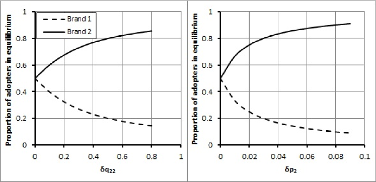
Figure 1: Proportion of adopters vs increments in the imitation and evaluation parameters respectively.

On the left chart of Fig. (1) we can observe that an increase in the coefficient of imitation strongly influences the final market proportion reached, so that for a 250% increase in $q_{22}$ (0.2 to 0.7), the final market share for this brand is approximately 80%. In the right chart it is shown that the effect due to an increase in parameter $p$ is similar (in percentage), where for a 250% increase in $p$ (from 0.01 to 0.035) the market share for brand 2 reaches 80% as well.

2.2.2 Cross-brand influence

We analyze the influence of the cross-terms $q_{ij}$ $(i\neq j)$ in the adoption dynamics given by the system of equations (3) and (4). To do so, the system was solved numerically with the Runge-Kutta method. In all calculations we considered the values ${}{}p_{1}=0.03$, $q_{1}=0.38$, $p_{2}=0.06$ and $q_{2}=0.68$, which are empirically reasonable according to ref. ([14]). The values of the cross-terms were chosen in order to make a systematic study, being then: A) $q_{12}=q_{21}=0,$ B) $q_{12}=0,$ $q_{21}=0.5,$ C) $q_{12}=0.5,$ $q_{21}=0$ and D) $q_{12}=0.5,$ $q_{21}=0.5$. Corresponding diffusion curves are shown in Fig. 2.

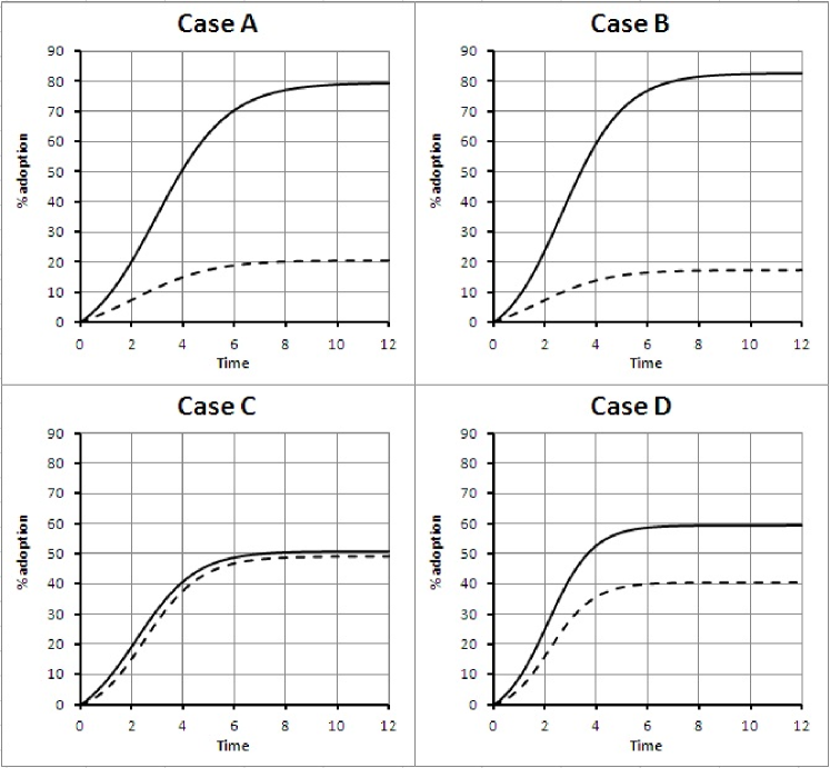
Figure 2: Study of the effect of cross-brand influence parameters. Brand 1 shown with dashed line and brand 2 with full line.

Case ”A” is a reference corresponding to when there not cross-brand influence. In the case ”B” by a non-zero value of $q_{21}$ the adoption of the brand 2 is reinforced, as a result accentuates the difference in the proportion of adopters of brand 2 compared to 1 in favor of the first. However this effect is not linear, as expected, principally when the full saturation with brand 2 is close. On the contrary by increasing the $q_{12}$ coefficient, such as we can appreciate in the case C, mainly tend to approach, this effect being stronger than the previous case of widening. It is interesting to note, that this effect would do compensate the advantage, of brand 2 over the other, due to better personal evaluation of the utility, making both brands finally have almost the same performance. Finally in the case D where both cross coefficients has the same value, a compensation of the effect produced in C occurs, i.e. some separation in the final proportion it is observed.

3 Agent-based model of innovation competition

The application of the ABMs to the study of the diffusion of innovations is currently a subject of great interest, as evidenced by the large amount of research work in this area (see for example [15], [16], [17], [18]). In these models the agents represent individuals who choose between two options: to adopt or not the new product.

The immediate physical analogy comes from thinking the agent as if it were a particle which can be in one of two states. As the system is constituted by a large number of ”particles” (agents), it is straightforward to think about applying statistical mechanics to its study. A similar system is the statistical Ising model, used in the field of physics. In this model the agents are atoms arranged in a regular network with two possible spin directions. The probability of finding an atom at a certain spin state can be described in thermodynamic equilibrium terms by the Boltzmann-Gibbs distribution [8]. However, we shouldn’t oversimplify by not taking into account the additional capacities that the agents present in real social systems, such as the learning possibility, the risk aversion, and also the free will to determine his contacts. The proposed model is used only as a formal frame that, due to its versatility, could be useful for the future introduction of the characteristics mentioned above.

In the analog physical problem there is a local and an external effect. The local effect is caused by the magnetic field produced by the neighborhood of the considered particle and an the external effect is due to the external field, which is not modified by the interaction with neighbors. In the social problem the local effect is due to the tendency to imitate the neighbors, and the external field is replaced by an individual assessment (or utility perception) made by each agent according to the qualities of product. However in the social context, the idea of neighborhood is somewhat vague, since the regular network is not usually the most appropriate way to describe the interaction.

A family of networks that are better suited for the description of social interaction processes is the one known as “small worlds networks” (SWN) [19]. Such networks may be constructed from a regular network by a rewiring method introduced by Watts and Strogatz [20]. This method implies rewiring the connections between agents by defining a parameter, called “probability of rewiring”, which is associated to each connection, thus making possible for each connection between neighboring agents to be broken and replaced with a connection between one of them to a random agent on the network.

In [7] there is a comparison between the diffusion curves coming from the Bass macroscopic model and from the ABM with the Ising model analogy. The impossibility of readoption is a characteristic of the Bass model, and as such, it was introduced in the ABM for the comparison’s sake. In [7] it is shown that for a given set of values of the Bass model’s parameters, the coincidence of the curves obtained from both models is almost perfect, an example is shown in Figure 3:

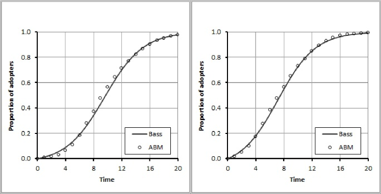
Figure 3: Example of the adoption curve match of an ABM and the Bass model.

The adjustment of the curve obtained using the ABM, using the software Mathematica 8 [21], was done by varying the parameters of the Bass analytical curve, which describes the solution of equation (3) when $q_{12}=0$, $p_{1}=p$, $q_{11}=q$, $n_{1}=n$ and $n_{2}=0$. That solution is:

$$n\left(t\right)=\frac{1-e^{-\left(p+q\right)t}}{1+\left(q/p\right)e^{-\left(p+q\right)t}}.$$ (39)

3.1 The three options algorithm

In [9] we proposed a formalism that allows us to treat problems that consider multiple options. It is based on an analogy of the generalization for more than two options of the Ising model (known as the Potts model). In the present article, this model is specialized for three options (i.e.; “brand 1”, “brand 2” and “non-adoption”). This allows us to propose the following decision algorithm, which is the probability of finding an agent in a given state (for null temperature). The example for state 1 is:

$$P\left(1\right)=\left\{\begin{array}[]{c}1\text{ if }\Delta_{1k}\text{ }>\text{ }0\text{ for }k=2,3\text{ \ \ \ \ \ \ \ \ \ \ \ \ \ \ \ \ \ \ \ \ \ \ \ \ \ \ \ \ \ \ \ \ \ }\\ 1/2\text{ if }\left\{\Delta_{12}=0\wedge\Delta_{13}>0\right\}\vee\left\{\Delta_{13}=0\wedge\Delta_{12}>0\right\}\\ 1/3\text{ if }\Delta_{12}=0\wedge\Delta_{13}=0\text{ \ \ \ \ \ \ \ \ \ \ \ \ \ \ \ \ \ \ \ \ \ \ \ \ \ \ \ \ \ \ \ \ }\\ 0\text{ if }\Delta_{12}<0\vee\Delta_{13}<0\text{ \ \ \ \ \ \ \ \ \ \ \ \ \ \ \ \ \ \ \ \ \ \ \ \ \ \ \ \ \ \ \ \ \ }\end{array}\right.,$$ (40)

with

$$\Delta_{kj}=\nu_{k}-\nu_{j}+u_{k}-u_{j},$$ (41)

for $k,j=1,2,3$.

The quantity $\nu_{j}$ is the proportion of agents in state $j$ within the agent’s contacts group, $u_{j}$ represents the utility of option $j$. The quantity $\Delta_{kj}$ can be interpreted as an effective utility, in which the first difference of Eq. (41) introduces the imitation effect, while the second difference compares the utilities of both.

4 Comparison between Bass and ABM for two brands in competition

In this section we will consider the adoption curves for two brands of an innovative product in competition for a given market. We will compare the results obtained by two very different models. In an way analogous to the calculation done in ref. [7], we will consider the adoption curve of an innovation obtained with an agent-based model (micro-level), and the curve obtained from the Bass model (macro-level).

As highlighted in the work [5] there is a dynamic influence on the adoption of one of the brands by the interaction with the adopters of the other brand, known as cross-brand effect. Mathematically this effect is introduced by means of the parameter $q_{ij}$ , as we saw in equations (3) and (4). From the perspective of the agent based model the cross-brand effect is not included. However it is interesting determine the magnitude of the cross brand effect.

4.1 Comparison for one brand

As shown in ref. [7], for the case considering one brand only, an almost perfect correspondence between the Bass model and the agent-based model can be established (see Figure 3). The adjustment of the Bass curve was made using Mathematica software [21]. The following data for the agent based model were used: utility difference between adopting or not $\Delta u=0.6$, rewiring probability $p_{r}=0$ (regular lattice), early adopters dispersion $\sigma$ = uniform, rate of incorporation of innovators (seeding) $\gamma=200$ per tick. The Bass curve was obtained using equation (39) with the parameters set to $p=0.0109$ and $q=0.3536.$These values are close to those determined by Bass [22] (for the unmodified model) for air conditioners in the USA. These are $p=0.0093$, $q=0.3798$, with errors of $0.0021$ and $0.0417$ respectively, which means the values obtained are empirically equivalent.

By increasing $\gamma$ until reaching $500$, which may be associated with a more aggressive advertising campaign, and leaving the other variables unchanged, we obtained the Bass parameter values $p=0.0239$ and $q=0.3513$, which fits the result of ABM as shown in Figure 3 on the right side.

4.2 Comparison for two brands in competition

The cases treated in isolation in the previous section will now be treated as two brands in competition. These involve, besides parameters $p$ and $q,$ a parameter associated with the cross-brand effect, as discussed in Section 2, i.e. $q_{ij}\neq 0$.

In the following sub-section we will investigate what can be inferred from the competition process between two brands. Our starting point will be our previous knowledge of the separate diffusion curves for each of the two brands in a monopolistic situation. The first case we will analyze is the ”minimal coincidence” one, in which the two models (Bass system and ABM) reach the saturation point with the same proportion of adopters.

4.2.1 Equilibrium proportions

The first test will compare the results coming from the Bass model with the ones coming from the ABM, particularly regarding the proportions of adopters of brands $1$ and $2$ (i.e. $n_{1}$ and $n_{2}$) at the saturation point. Let us consider two cases:

a) When we consider $q_{12}=q_{21}=0,$ the final proportion of adopters reached by the Bass system is $n_{1}=0.3155$ and $n_{2}=0.68446$, while with the ABM the result is $n_{1}=0.40125$ and $n_{2}=0.59875$.

b) For $q_{12}=q_{21}=0.077515$ we found that the coincidence with the ABM result reaches five decimal places. The value obtained for the cross-brand coefficients is within the range estimated in ref. [6], which may vary from zero to values up to the order of magnitude of the direct coefficients of the Bass system.

4.2.2 Diffusion curves

The following four numerical experiments were performed, which are shown in Fig. 4:

1) In Fig. 4A we show the diffusion curves of two brands in competition with the parameters $p$ and $q$ that we used before (in Fig. 3) to fit the monopoly cases. These are $p_{1}=0.0109$, $q_{11}=0.3536$ for the lower curve, and $p_{2}=0.0239$, $q_{22}=0.3513$ for the upper curve. In this case only the within-brand effect is taken into account, i.e., $q_{12}=q_{21}=0$. We see that the results for both models are very different.

2) Now we take into account the cross-brand effect, but restricted to $q_{12}=q_{21}$. We use the value that produces the best fit for the final proportion of the adopters whic, as we saw in sub-section 4.2.1, is $q_{12}=q_{21}=0.0775$. All other parameters remain the same as in the last case. The result is shown in Fig. 4B where there’s an $8.04\%$ difference between the areas under the curves.

3) As in the previows case, only the cross coefficients are modified, but now without the imposed restriction. We use the values that better approximate the curves coming from the ABM model wihtout changing the final equilibrium. The result is shown in Fig. 4C. The difference between areas is now $5.86\%$ and the values of the coefficients are $q_{12}=0.047$ and $q_{21}=0$.

4) In this experiment all the parameters are freely changed until reaching an excellent fit between the curves, as we can appreciate in Fig. 4D. The values obtained are: $p_{1}=0.0023$, $q_{11}=0.5787$, $p_{2}=0.0125$, $q_{22}=0.4252$, $q_{12}=0.0293$ and $q_{21}=0.0009$. The difference of area obtained is $1.59\%$ and the fit coefficients for the curves 1 (the lower) and 2 (the upper) respectively are: $R_{1}^{2}=0.9987$ and $R_{2}^{2}=0.9993$.

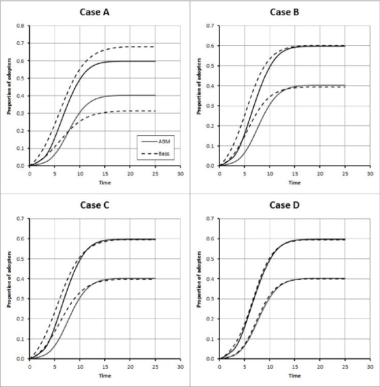
Figure 4: Comparisson between two diffusion models of two brands competing in a common market : AMB and Bass system, with different aproximations by the variation of cross-brand coefficients.

5 Conclusions and discussion

As a general conclusion we have seen that the cross-brand coefficients of the Bass system cannot be both zero if we want to fit the synthetic curves obtained from an ABM inspired in the Potts statistical model.

In particular we highlight the following results:

• Assuming that all Bass system coefficients are positive, the only equilibrium points are those that are on the straight line $n_{2}=1-n_{1}$ with $n_{1}>0,n_{2}>0$, which correspond to all the cases where the market is saturated. The system is in indifferent equilibrium over this straight line, in such a way that if we disturb the equilibrium and let the system evolve freely, the result tends to return to the line. Hence, we can say the line acts as an attractor.

• For a minimal coupling of the system, that is, when only within-brand influence is considered, it is possible to derive an analytical relationship between the equilibrium points and the Bass coefficients. We see that both personal evaluation and the rate of imitation strongly influence the market share achieved at market saturation.

• The effect of the cross-brand parameters is stronger when the coefficient favors the brand with less utility (brand 1). So while a high value of $q_{21}$ (such as $q_{21}=0.5$) increased the final $n_{2}$ in less than $3\%$, a $q_{12}=0.5$ had a great influence, such that $n_{1}\sim n_{2}$ in the final equilibrium.

• Regarding the comparison with the agent based model, we see that by considering $q_{12}=q_{21}=0.077515$ the same result, in terms of the final proportions, is obtained for both brands even though in the ABM there is nothing comparable to the cross-brand terms of the Bass system equations.

• The best fit for the diffusion curves obtained from both models is reached when all the parameters of the Bass model are set free. We can therefore conclude that the probabilities of innovation and imitation, represented by $p$ and $q$ in the Bass model, depend on the competition between brands. Therefore it is not correct to fix those coefficients a priori, using only diffusion curves for the brands in a monopolistic market. As a conclusion, we can say that cross-brand coefficients must be not null for a proper fit.

These results leave some questions to be answered. In the first place we can ask ourselves; why is it necessary to include the cross-brand terms $q_{{}_{jk}}\left(j\neq k\right)$, in the Bass system, in order to reproduce the ABM curves?. As we have seen, it is not enough to consider the parameters obtained from the monopolistic case to describe the duopolistic one. Even when they provide a very good fit for the diffusion of both brands as a monopoly, it is still necessary to include the cross-brand terms to accurately model the diffusion of two brands in competition. This means that in the ABM used there is something that models the cross brand effect, even if it doesn’t present any parameter equivalent to the cross-brand terms of the Bass system. But, why?, does the ABM include a positive influence towards the adoption of a brand via those agents that have adopted the other brand?. The answer is yes. To realize this it is necessary to center in the algorithm given in Eq. (40).

Let us think in a given agent that evaluates the possibility to adopt brand 1. The probability of adoption will be $P(1)$, given by Eq. (40). Let us consider, for simplicity’s sake, a didactic example in which both, products 1 and 2, have the same utility as the non-adoption option (state 3). Considering this, Eq. (41) will be $\Delta_{kj}=\nu_{k}-\nu_{j}$. Let us also consider that the agent is connected to 8 neighbours within a regular network. We will compare two situations: (i) half the neighbours adopt brand 1 and the other half remains non-adopter and (ii) half the neighbours adopt brand 1, a quarter of the neighbours adopt brand 2 and the remaining quarter remains non-adopter. In case (i) we’ll have $\Delta_{12}=1/2$ and $\Delta_{13}=0$ which means $P(1)=1/2$, while case (ii) presents $\Delta_{12}=1/4$ and $\Delta_{13}=1/4$ which means $P(1)=1$.

In this example we can see that even if in both cases half the neighbourhood has adopted brand 1, in the second case brand 1 has been promoted by the agents that adopted brand 2. In other words we can say that there’s an influence in imitation at the category level, which seems reasonable according to empirical data showing that the introduction of a new brand in the market helps the diffusion existing analogous of the brand in the context of innovations, as shown in ref.[5]. This explains why it is necessary to include the cross brand terms in the Bass system to compare it with the ABM used.

Another question that arises from the results is; why is it not enough to include the cross-brand terms to reach the best fit?.

We saw that using the best fit parameters for the monopolistic level plus the cross-brand parameters isn’t enough to achieve the best fit in the duopolistic level. We need to free all of Bass parameters to do it.

This result is also explained by the kind of coupling between imitation and cross-brand effect, which allows us to directly relate the macroscopic Bass parameters to the microscopic ABM ones.

In the Bass system the $q_{{}_{ii}}$, related to the imitation probability, are independent from the $q_{{}_{jk}}$. Nevertheless, in the ABM, as seen in the previous example, the adoption of brand 2 boosts adoption of brand 1, which implies that, in relative terms, the imitation effect seems stronger. This dependence among the causers of adoption in the ABM means that, when adjusting the Bass model, the coefficients $q_{{}_{ii}}$ also become dependent of the $q_{{}_{jk}}$, which is why it is necessary to let them free to allow for a mutual compensation in the best fit.

Future investigations could focus on relaxing some of the hypotheses used in the present paper, in order to achieve a higher degree of realism. For example, the conclusions we arrived to are subject to the supposition that agents are homogeneous in their evaluation of both brands; we could nevertheless suspect that the personal evaluation each person performs will depend on his social status and that the interpersonal influences could have a different weight depending on whether they are between agents of similar social groups (homophily) or different social groups (heterophily) [23]. Recently, in ref. [24] we can even find the possibility of insertion of a product with an asymmetric attraction/repulsion, reflected by a negative sign on one of the cross-brand coefficients. These interesting ideas should be explored and will undoubtedly be subject of future investigations.

6 Appendix

The purpose of this appendix is to establish relationships between the proportions $n_{1}$ and $n_{2}$ and the parameters $p_{1}$, $p_{2}$, $q_{11}$ and $q_{22}$, when $q_{12}=q_{21}=0$.

We begin performing the quotient of Eqs. (36) and (37). After that, we reorganize the terms in the form:

$$\frac{dn_{2}}{p_{2}+q_{22}n_{2}}=\frac{dn_{1}}{p_{1}+q_{11}n_{1}},$$ (A1)

by integrating we obtain:

$$\frac{1}{q_{22}}\ln\left(p_{2}+q_{22}n_{2}\right)=\frac{1}{q_{11}}\ln\left(p_{1}+q_{11}n_{1}\right)+C.$$ (A2)

To determine the integration constant $C$ we will use the fact that Eq. (2) holds at all times, in particular for the initial time, but we will assume that the initial ratio is zero or $n_{1}(0)=n_{2}(0)=0$. Thus by specializing of Eq. (A2) at $t=0$ and solving for $C$ we get

$$C=\frac{1}{q_{22}}\ln p_{2}-\frac{1}{q_{11}}\ln p_{1},$$ (A3)

By replacing Eq. (A3) in Eq. (A2) and rearranging we have

$$\ln\left(1+\frac{q_{22}}{p_{2}}n_{2}\right)=\ln\left[\left(1+\frac{q_{11}}{p_{1}}n_{1}\right)^{\frac{q_{22}}{q_{11}}}\right].$$ (A4)

Exponentiating Eq. (A4) is

$$1+\frac{q_{22}}{p_{2}}n_{2}=\left(1+\frac{q_{11}}{p_{1}}n_{1}\right)^{\frac{q_{22}}{q_{11}}}.$$ (A5)

As Eq. (A5) holds at all times, in particularly for the equilibrium, that is when is valid the following equation

$$n_{2}=1-n_{1}.$$ (A6)

Substituting Eq. (A6) in Eq. (A5) yields Eq. (38) which is shown in subsection 2.2.1.

Acknowledgement 1

This research was supported partially by two U.S. National Science Foundation (NSF) Coupled Natural and Human Systems grants (0410348 and 0709681) and by the University of Buenos Aires (UBACyT 00080).

References

- [1] Mahajan, V., Muller, E., Wind, Y., New-Product Diffusion Models, Kluwer Academis Press, 2000.
- [2] Meade, N., Islam, T., Modelling and forecasting the diffusion of innovation-A 25-year review: twenty five years of forecasting, International Journal of Forecasting 22 (2006) 519-545.
- [3] Peres, R., Muller, E., Mahajan, V. (2010). Innovation diffusion and new product growth models: A critical review and research directions. International Journal of Research in Marketing 27, 91-106.
- [4] Bass, F. M. (1969). A new product growth for model consumer durables. Management Science 15: 215-227.
- [5] Libai, B., Muller, E., Peres, R.(2009). The Role of Within-Brand and Cross-Brand Communications in Competitive Growth. Journal of Marketing 73: 19-34.
- [6] Savin, S., Terwiesch, C. (2005). Optimal Product Launch in a Duopoly: Balancing Life-Cycle Revenues with Product Cost. Operations Research 53, No 1, 26-47.
- [7] Laciana, C. E., Rovere, S. L., and Podestá, G. P., (2013). ”Exploring associations between micro-level models of innovation diffusion and emerging macro-level adoption patterns”. Physica A 392, 1873-1884.
- [8] Laciana, C.E., and Rovere, S.L., (2011). “Ising-like agent-based technology diffusion model: adoption patterns vs. seeding strategies,” Physica A, vol. 390, no. 6, pp. 1139-1149.
- [9] Laciana, C. E., and Oteiza-Aguirre, N., (2014). ”An agent based multi-optional model for the diffusion of innovations”, Physica A 394, 254-265.
- [10] Wu, F. Y., (1982). ”The Potts model”. Reviews of Modern Physics, Vol. 54, No 1, pp. 235-265.
- [11] Sengupta, A., Greetham, D. V., and Spence, M.. ”An Evolutionary Model of Brand Competition”. Proceedings of the 2007 IEEE Symposium on Artificial Life (C1-Alife 2007).
- [12] Casillas, L., Espinosa, F.J., Huerta-Quintanilla, R. and Rodriguez-Achach, M., (2006). ”Condensation in an economic model with brand competition”. Int. Journal of Modern Physics C, Vol. 17, No 5, pp. 749-756.
- [13] Kalish, S., Mahajan, V., and Muller, E., (1995). ”Waterfall and sprinkler new-product strategies in competitive global markets”. Intern. J. of Research in Marketing, Vol. 12, 105-119.
- [14] Sultan, F., Farley, J.U., and Lehmann, D.R., (1990). ”A Meta-Analysis of Applications of Diffusion Models”. J. of Marketing Research, Vol. XXVII, pp. 70-77.
- [15] Olaru, A., and Florea, A.M., (2009).”Emergence in Cognitive Multi-Agent Systems”, in : International Conference on Control Systems and Computer Science, Bucharest, Romania.
- [16] Schramm, M.E., Trainor, K.J., Shanker, M., and Hu, M.Y. (2010). ”An agent-based diffusion model with consumer and brand agent”. Decision Support Systems 50, 234-242.
- [17] Chatterjee, J., and Eliasberg, J. (1990). ”The innovation diffusion process in a heterogeneous population: a micromodeling approach”. Management Science 36, 1057-1079.
- [18] Goldenberg, J., and Efroni, S. (2001). ”Using cellular automata modeling of the emergence of innovations”. Technological Forecasting and Social Change 68, 293-308.
- [19] Watts, D.J. (1999). ”Small Worlds”, Princeton University Press.
- [20] Watts, D.J., and Strogatz, S.H., (1998). “Collective dynamics of ‘small-world’ networks,” Nature, vol. 393, pp. 440-442.
- [21] Wolfram Research, Mathematica (1988).
- [22] Bass, F.M., Krishnan, T.V., and Jain, D.C.(1994). ”Why the Bass model fits without decision variables”. Marketing Science 13, 203-223.
- [23] Li, Y., Wu, C., Peng,L., and Zhang, W. (2013). ”Exploring the Characteristics of Innovation Adoption in Social Networks: Structure, Homophily, and Strategy”. Entropy, vol.15, pp. 2662-2678.
- [24] Bakshi, N., Hosanagar, K., & Van den Bulte, C. (2013). ”Chase and Flight: New Product Diffusion with Social Attraction and Repulsion”. History, pp. 1-31.