First exact Geon found is a non-singular monopole, propagating as a primordial gravitational pp-wave.

Nikolaos A. Batakis

Department of Physics, University of Ioannina,

45110 Ioannina, Greece

(nbatakis@uoi.gr)
July 10, 2014

Abstract

Geons are particle-like electrovacua. The concept is well-defined, but it still lacks a proper first example. Emerging as such is a self-confined exact 2-parameter pp-wave non-Dirac monopole ${\cal G}$ with primordial $Q/r^{2}$ ($r\geq r_{o}$) field plus higher moments. ${\cal G}$ has effective mass, independently-scaled NUT-like charge $\kappa|Q|=2r_{o}$ as diameter, and spin. ${\cal G}$ cannot have actual em charge $Q$ (by $\partial{\cal G}=0$), Ricci-flat limits, nor spacetime or Dirac-string singularities, but Dirac’s quantization condition holds. ${\cal G}/2$, as an upgraded ‘Kerr-Newman’ alternative or ${\cal S}_{Q}$ geon, carries actual charge $Q$ confined by topology on a round-$S^{2}[r_{o}]$ physical singularity on $\partial{\cal S}_{Q}\neq 0$. ${\cal G}$ and ${\cal S}_{Q}$ offer exact analytic models in particle physics and cosmology, notably for primordial gravitational waves, inflation, and pre-galactic dynamics.

$\@@underline{\hbox{PACS numbers}}$: 04.20.Cv, 04.20.Jb., 11.10.-z.
$\@@underline{\hbox{Key words}}$: Geon, electrovacuum, NUT charge, pp-wave soliton, primordial field, non-Dirac monopole, ‘Kerr-Newman’, primordial gravitational wave, inflation, pre-galactic dynamics.

[file: Geons]

1 Introduction

A century-old interest on ‘small particles’ made of self-confined spacetime was alerted by Schwarzschild’s 1915 solution and evolved all the way into the 50s, with Einstein’s own among widespread efforts to uncover non-singular particle-like vacua or electrovacua [1][2][3]. Epitomized as Geon by Wheeler [4], the concept still lacks a proper first example, namely a sufficiently stable and self-confined exact non-singular solution of Einstein’s gravity coupled to sourceless Maxwell fields. The closest we’ll ever come to exact pure-vacuum geons, which would actually require exotic topologies [3], might well be the Taub-NUT (albeit effectively massless) vacuum [5]. This remarkable space, tediously assembled as nut-t-nut from the Taub and NUT vacua, and several decades since, remains the only known exact non-singular (and with no boundaries) Ricci-flat space with ${\cal S}=S^{3}\times{\rm I\kern-1.79993ptR}$ topology [6][7]. So, conclusively, we actually have only approximations to desirable 4D geon electrovacua [8]. Meanwhile, the notorious lack of exact solutions (plus concern for stability) has refocused interest back to singular models via topological geons [9], and toward the quantum-mechanical properties of geon black holes or Reissner-Nordström versions of Taub-NUT [7]. Here, a 2-parameter family of primordial self-confined pp-wave non-Dirac monopoles with $Q/r^{2}$ ($r\geq r_{o}$) field, the ${\cal G}={\cal S_{-}}\vee{\cal S_{+}}$, is proposed as the first exact geon. The ‘${\cal G}/2$’ or ${\cal S}_{Q}$ geon has actual $Q$-charge confined topologically over a round $S^{2}[r_{o}]$ on the $\partial{\cal S}_{Q}\neq 0$ physical singularity.

Geons already have substantial applications, as noted. However, if allowed (as a concept) to be singular, they would have to be excluded from their expectedly most important and natural presence, namely at the Big Bang, immediately after the first quantum fluctuation(s) of the vacuum. There, with inflatons as a suspended exception, the only physical entity which could have existed is the graviton as a primordial gravitational-wave particle. Proposed as analytic model for the latter, our primordial (Big-Bang) ${\cal G}_{\rm bb}$ pp-wave geon will be outlined as last example in the last section. So we begin with the Hilbert-Einstein Lagrangian for gravity, coupled by $\kappa$ to sourceless-Maxwell content in

$${\cal L}=\frac{1}{\kappa^{2}}\varepsilon_{\alpha}^{\;\beta}\,{\cal R}^{\alpha}_{\;\beta}-F\wedge\ast F\,,$$ (1.1)

to uncover ${\cal G}$ as a particle-like manifold with electromagnetic (em) content $F$. Symmetries make ${\cal G}$ a Bianchi-type IX (left-$SU(2)$ invariant), with an extra Killing vector $\partial_{\psi}$ for axial rotations $\psi\in[0,4\pi)$ as the only survivor of right-$SU(2)$ invariance. A non-singular ${\cal G}$ cannot carry actual mass $m_{G}$. It can neither have actual em charge $Q$, by $\partial{\cal G}=0$ and $dF=d\ast F=0$ from (1.1). Such aspects can here emerge only a posteriori, effectively or otherwise, if at all.

2 A preview of the geometry and content of ${\cal G}$

The line element of ${\cal G}$ can be set as a Taub-NUT type in terms of left-$SU(2)$ invariant 1-forms $\ell^{i}$ (from $\theta,\phi,\psi$ angles on $S^{3}$), scaled by ${\rm L_{o}}$, with $g=g(u)$, $r=r(u)$ functions of $u\in{\rm I\kern-1.79993ptR}$ in

$$ds^{2} = -{\rm L_{o}^{2}}\left(g\ell^{3}+2du\right)\ell^{3}+r^{2}d\Omega^{2}\,,\;\;\;\;d\Omega^{2}\!\!:\,=(\ell^{1})^{2}+(\ell^{2})^{2}=d\theta^{2}+\sin^{2}\theta\;d\phi^{2},\;\;\;$$ (2.1)

$$\ell^{1}=\cos\psi d\theta+\sin\psi\sin\theta\,d\phi,\;\;\;\ell^{2}=-\sin\psi d\theta+\cos\psi\sin\theta\,d\phi,\;\;\;\ell^{3}=d\psi+\cos\theta\,d\phi\,.$$ (2.2)

The $L_{i}$, as duals of $\ell^{i}$ in $<\!\!\ell^{i}|L_{j}\!\!>=\delta^{i}_{j}$, obey $<\!\!\ell^{i}|[L_{j},L_{k}]\!\!>=\epsilon^{i}_{jk}$ via the equivalence of

$$d\ell^{i}\!=\!-\frac{1}{2}\epsilon^{i}_{jk}\ell^{j}\wedge\ell^{k}\;\;\;\longleftrightarrow\;\;\;\;[L_{j},L_{k}]=\epsilon^{i}_{jk}L_{i}\,,$$ (2.3)

with, as we read off (2.1), $(L_{1})^{2}=(L_{2})^{2}=r^{2}$, $(L_{3})^{2}=-g{\rm L_{o}^{\,2}}$, $\partial_{u}^{\,2}=0$, $L_{3}\cdot\partial_{u}\!=\!-{\rm L_{o}^{\,2}}$, etc, including the $\partial_{u}$ null vector. Einstein’s equations in orthonormal Cartan frames [2], to make (2.1) locally manifest-Lorentz with $\eta_{\alpha\beta}={\rm diag}[-1,1,1,1]$ ($\alpha=0,i$), will emerge as

$$R_{\alpha\beta}=\kappa^{2}\,T_{\alpha\beta}^{\rm({\sc em})},\;\;\;\;\;\;\;T_{\alpha\beta}^{\rm({\sc em})}=\frac{E^{2}+B^{2}}{2}\left[\begin{array}[]{cccc}1&0&0&0\\ 0&1&0&0\\ 0&0&1&0\\ 0&0&0&-1\end{array}\right],$$ (2.8)

namely sourced by em content $T_{\alpha\beta}^{\rm({\sc em})}$ in ${\cal G}$, a manifest locally-Minkowski $M^{4}_{\!o}$ in those frames. The scaleless $u\in{\rm I\kern-1.79993ptR}$ null coordinate will be used as global time for now, to be shortly redefined as $t$ and later-on as $\rho$. To preview the geometry and how ${\cal G}$ acquires particle-like size from the $r=r_{o}$ minimum, we need the $r=r(u)$, $g=g(u)$; they’ll emerge from (2.8) as

$$r^{2}=r_{o}^{2}+{\rm L_{o}^{2}}Pu^{2}\,,\;\;\;g=\frac{1}{P}\,,\;\;\;\;\;\;\;\;\;\;\;\left[2r_{o}=\frac{\rm L_{o}}{\sqrt{P}}=\kappa|Q|\right],$$ (2.9)

in terms of the scaleless $P>0$ and $Q\neq 0$ constant parameters. Thus, ${\cal G}$ and Taub-NUT share type of metric, scale ${\rm L_{o}}$ and all isometries in (2.1), plus invariance under

$$u\rightarrow-u\,,\;\;\;\;\;u\rightarrow u+u_{o}$$ (2.10)

reflections and translations of $u$. They also share the spacelike radius $r$ of $S^{3}$ as $r=r(u)$ function with $\pm{\rm L_{o}}\sqrt{P}u$ asymptotes in (2.9) and (2.11), all depicted in diagram (i) of Fig.1.

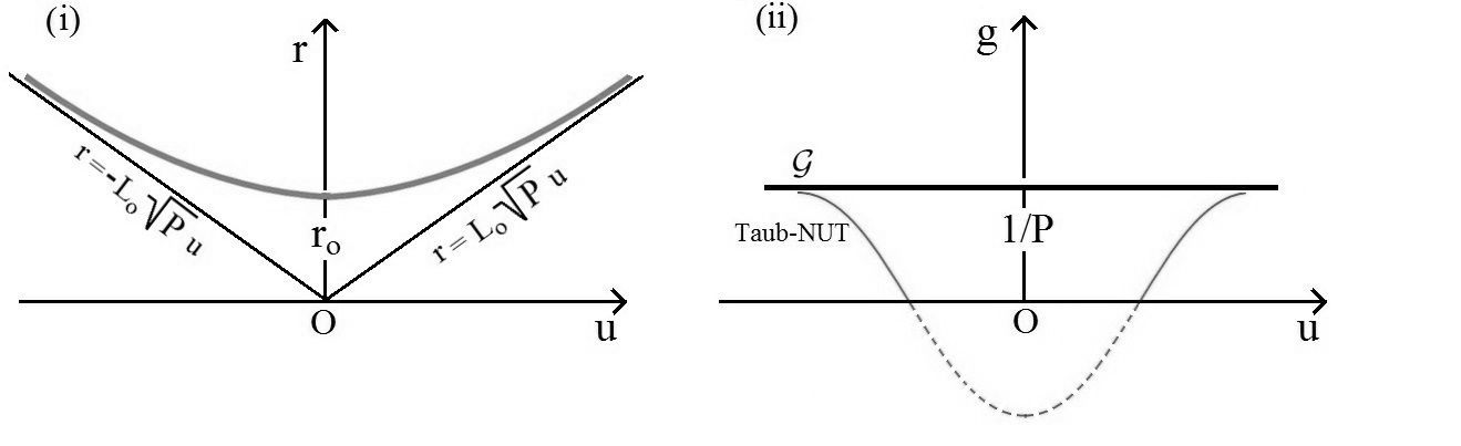
Figure 1: ${\cal G}$ vs Taub-NUT. (i) Both have the same $r=r(u)$ function on $\pm{\rm L_{o}}\sqrt{P}u$ asymptotes and $r_{o}$ minimum at $u=0$, Planck-scaled in ${\cal G}$ as a $2r_{o}=\kappa|Q|$ NUT-like charge. (ii) ${\cal G}$ has constant $g(u)=1/P$, thus timelike $L_{3}$ $\forall u$, hence no Taub sector (dashed) or Misner bridges.

These strong similarities do not inhibit stronger differences, by which ${\cal G}$ cannot even reduce to a Taub-NUT. Actually, ${\cal G}$ is forbidden to reduce to any Ricci-flat or singular limit, because the $2r_{o}=\kappa|Q|$ NUT-like charge cannot vanish. ${\cal G}$ also carries the $\kappa^{2}=8\pi G_{\rm N}$ scale and the $Q$ (electric or magnetic) charge parameter, with no counterpart in the also 2-parameter Taub-NUT. The latter’s NUT charge as $2r_{o}={\rm L_{o}}/\sqrt{P}$ is fundamentally different from the (formally identical) NUT-like charge $2r_{o}={\rm L_{o}}/\sqrt{P}$ as a diameter in ${\cal G}$. The point (and third difference) here is that in ${\cal G}$ we also have $2r_{o}=\kappa|Q|$ (a geometric-mean of couplings, if $Q^{2}\sim 1/137$) as a second equivalent expression. The fourth difference is crucial: $g(u)$ in ${\cal G}$ is by (2.9) a $g=1/P>0$ constant, approached only asymptotically by $g=g(u)$ in Taub-NUT, as shown in diagram (ii) of Fig.1, Thus, by $(L_{3})^{2}=-(2r_{o})^{2}$, $L_{3}$ is timelike everywhere in ${\cal G}$. As a result, Taub sector and Misner bridges, vital as they have been to keep Taub-NUT ‘standing’, do not exist in ${\cal G}$, as if em content had filled-in for ‘support’. Accordingly, ${\cal G}$ consists of two NUT-like pieces ${\cal S_{\pm}}$ in $C^{\infty}$ junction at $u=0$ (with ${\cal S_{+}}\leftrightarrow{\cal S_{-}}$ under $u\leftrightarrow-u$), as a ${\cal G}={\cal S_{-}}\vee{\cal S_{+}}$, sort of a nut-t-nut with the Taub removed. The ${\cal S_{\pm}}$ propagate as gravito-em solitons along the null $\pm\partial_{u}$ wave vector, which obeys the $D\partial_{u}=0$ pp-wave condition. ${\cal S_{-}}$ propagates backwards in time, towards $r\rightarrow-{\rm L_{o}}\sqrt{P}u$ in (i) of Fig.1, as an antisoliton. The inverse of $r=r(u)$ in (2.9) is a double-valued $u=u(r)$ function

$$u=\pm\frac{1}{{\rm L_{o}}\sqrt{P}}\sqrt{r^{2}-r_{o}^{2}}\;\;\;\;\;\stackrel{{\scriptstyle r>>r_{o}}}{{\longrightarrow}}\;\;\;\;\;\;\;\;\;u=\pm\frac{1}{{\rm L_{o}}\sqrt{P}}\;r\;\;\rightarrow\;\;r={\rm L_{o}}\sqrt{P}\,|u|,$$ (2.11)

with a double-valued limit at $r>>r_{o}$, so $r$ cannot cover ${\cal G}$ globally. This gives rise to the notion of a ${\cal G}/2=\!{\cal S}_{Q}$ geon as a manifold covered globally by $r$, inevitably with $\partial{\cal S}_{Q}\neq 0$. This boundary at $r=r_{o}$ (the former junction at $u=0$) is a squashed-$S^{3}$ physical singularity with a round-$S^{2}[r_{o}]$ spacelike section of diameter $2r_{o}=\kappa|Q|$. The $r>>r_{o}$ limit in (2.11) is a null-cone, depicted in (i) of Fig.1 as asymptotes, whose $r\geq 0$ range in tangent space is clearly distinct from the $r\geq r_{o}$ range in ${\cal G}$ or ${\cal S}_{Q}$, wherein the $r=r_{o}$ minimum is a perfectly regular point (cf., next section). We can now trade manifest left-$SU(2)$ invariance in (2.1), using (2.2) and (2.11), for global $t$-time defined by $\sqrt{P}t={\rm L_{o}}(\psi+Pu)$ in

$$ds^{2} = -\left(dt+2r_{o}\cos\theta d\phi\right)^{2}+\frac{r^{2}}{r^{2}-r_{o}^{2}}(dr)^{2}+r^{2}\left(d\theta^{2}+\sin^{2}\theta d\phi^{2}\right),$$ (2.12)

$$dt = {\rm L_{o}}\left(\frac{1}{\sqrt{P}}d\psi+{\sqrt{P}}du\right)=2r_{o}\left(d\psi+Pdu\right)\,.$$ (2.13)

The em content of gauge potentials and $F=dA$ fields in ${\cal G}$ and ${\cal S}_{Q}$ is also non-singular everywhere (c.f., sections 3,4). As first of two cases, an ‘electric’ type $F^{\rm(e)}=dA^{\rm(e)}$ in

$$A^{\rm(e)}=\frac{Q\sqrt{r^{2}-r^{2}_{o}}}{r^{2}}\,\left(dt+2r_{o}\cos\theta\,d\phi\right)\;\longrightarrow\;\;E^{\rm(e)}=\frac{Q}{r^{2}}+O(r^{-4})\,,\;\;B^{\rm(e)}\sim O(r^{-3}),$$ (2.14)

in holonomic $(t,r,\theta,\phi)$ coordinates from (2.12), has a dominant electric-monopole $E_{C}=Q/r^{2}$ field in $E^{\rm(e)}$ plus electric and magnetic higher-order terms. Equally acceptable is the

$$A^{\rm(m)}=-\frac{Q(r^{2}-2r_{o}^{2})}{2r_{o}r^{2}}\,\left(dt+2r_{o}\cos\theta\,d\phi\right)\;\longrightarrow\;\;E^{\rm(m)}\sim O(r^{-3})\,,\;\;B^{\rm(m)}=\frac{Q}{r^{2}}+O(r^{-4})\;\;$$ (2.15)

‘magnectic’ type $F^{\rm(m)}=dA^{\rm(m)}$, with a dominant magnetic-monopole $B_{C}=Q/r^{2}$ field in $B^{\rm(m)}$ plus higher-order terms, with $F^{\rm(m)}=\ast F^{\rm(e)}$ by em duality. We recall that actual charge $Q$ in ${\cal G}$ is forbidden by $dF=d\ast F=0$ and $\partial{\cal G}=0$, so those $Q/r^{2}$ fields in ${\cal G}$ are primordial. ${\cal S}_{Q}$, however, must carry actual surface-charge $\sigma_{Q}$ trapped by topology on a round-$S^{2}[r_{o}]$ in $\partial{\cal S}_{Q}\neq 0$ (c.f., section 4). Particular choices of the $P,Q$ parameters can involve very different physical profiles and scales in a non-susy hierarchy in the $r\geq r_{o}$ range of radii. Depending on $|Q|$, we can have a Planck-scale (or even smaller) $2r_{o}=\kappa|Q|\sim\kappa$ in a 4-scale hierarchy, up to a relatively enormous $2r_{o}=\kappa|Q|\sim r_{\rm sm}$ minimum in a 3-scale hierarchy, as

$$r_{o}\sim\kappa|Q|\sim\kappa<<r_{\rm sm}<<r_{\rm cl}<<r_{\infty}\,,\;\;\;\;\;\;\;\;\;\;r_{o}\sim\kappa|Q|\sim r_{\rm sm}<<r_{\rm cl}<<r_{\infty}\,,\;\;\;\;\;$$ (2.16)

namely a Planck-length $r_{o}\sim\kappa$ (4-scale case), vs a standard-model (below $10^{16}$ Gev) length as $r_{o}\sim r_{\rm sm}$ (3-scale case); common to both cases are the $r\sim r_{\rm cl}$ scale (a mean free path) and $r\sim r_{\infty}$ (a Hubble radius) within a Friedman model ${\cal F}$ filled with ${\cal G}$-geons.

3 The general non-singular solution for ${\cal G}$

We can re-express (2.1) as $ds^{2}=\eta_{\alpha\beta}\theta^{\alpha}\theta^{\beta}$ with 1-forms (plus duals) in $<\!\!\theta^{\alpha}|\Theta_{\beta}\!\!>=\delta^{\alpha}_{\beta}$ as Cartan frames in non-singular geometry [2], which are chosen in terms of $du,\ell^{i}$ as

$$\theta^{0} = {\rm L_{o}}\left(\sqrt{P}du+\frac{1}{\sqrt{P}}\ell^{3}\right),\;\;\;\theta^{1}=r\ell^{1},\;\;\;\theta^{2}=r\ell^{2},\;\;\;\theta^{3}={\rm L_{o}}\sqrt{P}du,$$ (3.1)

$$\Theta_{0} = \frac{\sqrt{P}}{\rm L_{o}}L_{3},\;\;\;\Theta_{1}=\frac{1}{r}L_{1},\;\;\;\Theta_{2}=\frac{1}{r}L_{2},\;\;\;\Theta_{3}=\frac{1}{\rm L_{o}}\left(\frac{1}{\sqrt{P}}\partial_{u}-\sqrt{P}L_{3}\right),$$ (3.2)

so they are also manifest left-$SU(2)$ invariant. After the $D\theta^{\alpha}\!:\,=d\theta^{\alpha}+\Gamma^{\alpha}_{\;\beta}\wedge\theta^{\beta}=0$ definition for the covariant derivative, we can easily verify the claimed $D\partial_{u}=0$ pp-wave condition, while the (here non-holonomic) Christoffel $\Gamma^{\alpha}_{\;\beta\gamma}\theta^{\gamma}=\Gamma^{\alpha}_{\;\beta}$ 1-forms follow as

$$\Gamma_{\alpha\beta} = -\Gamma_{\beta\alpha}:\;\;\;\;\;\;\;\;\;\;\Gamma_{01}=\frac{\rm L_{o}}{2\sqrt{P}r^{2}}\,\theta^{2},\;\;\;\;\Gamma_{02}=-\frac{\rm L_{o}}{2\sqrt{P}r^{2}}\,\theta^{1},\;\;\;\;\Gamma_{03}=0,$$ (3.3)

$$\Gamma_{12} = -\frac{\sqrt{P}}{\rm L_{o}}\left(1-\frac{\rm L_{o}}{2\sqrt{P}r^{2}}\right)\theta^{0}+\frac{\sqrt{P}}{\rm L_{o}}\,\theta^{3},\;\;\;\;\Gamma_{23}=\frac{\dot{r}}{\rm L_{o}\sqrt{P}r}\,\theta^{2},\;\;\;\;\Gamma_{31}=-\frac{\dot{r}}{\rm L_{o}\sqrt{P}r}\,\theta^{1},$$

with a dot for $d/du$. The curvature ${\cal R}^{\alpha}_{\;\beta}=\frac{1}{2}R^{\alpha}_{\;\beta\gamma\delta}\theta^{\gamma}\wedge\theta^{\delta}=d\Gamma^{\alpha}_{\;\beta}+\Gamma^{\alpha}_{\;\gamma}\wedge\Gamma^{\gamma}_{\;\beta}$, which also supplies Ricci’s $R_{\alpha\beta}=R^{\gamma}_{\;\alpha\gamma\beta}$, gives Riemann’s contractible components, all non-singular as

$$R^{0}_{\,101}=R^{0}_{\,202}=-\frac{\rm L_{o}^{2}}{4Pr^{4}},\;R^{1}_{\,212}=-\frac{1}{\rm L_{o}^{2}P}\left(\frac{\dot{r}}{r}\right)^{\!2}+\frac{4Pr^{2}+3{\rm L_{o}^{2}}}{4Pr^{4}},\;R^{1}_{\,313}=R^{2}_{\,323}=-\frac{1}{{\rm L_{o}^{2}}P}\frac{\ddot{r}}{r},$$ (3.4)

and Weyl’s one independent component as $2PW_{0123}=-PW_{0312}=\dot{r}/r^{3}$, vanishing as $O(r^{-3})$. By (1.1),(2.8) etc, $F=\frac{1}{2}F_{\alpha\beta}\,\theta^{\alpha}\!\wedge\theta^{\beta}$ can only have $F_{03}$ and $F_{12}$ components as

$$F=-E\,\theta^{0}\wedge\theta^{3}+B\,\theta^{1}\wedge\theta^{2}\,,\;\;\;\ast F=B\,\theta^{0}\wedge\theta^{3}+E\,\theta^{1}\wedge\theta^{2}\,.$$ (3.5)

With $\rho$-time defined via $r^{2}\dot{\rho}={\rm L_{o}^{2}}$ in $d\ast dA=0$, the general solution is non-singular as

$$A=\frac{Q\sqrt{P}}{\rm L_{o}}\sin(\rho+\rho_{o})\;\theta^{0}\;,\;\;\;\;\;\;\;\;\left[r^{2}d\rho={\rm L_{o}^{2}}du\right],$$ (3.6)

with $\rho_{o}$ a duality-rotation angle, supplying us with either of $F^{\rm(e)}$ or $F^{\rm(m)}=\ast F^{\rm(e)}$ from

$$A^{\rm(e)}=\frac{Q\sqrt{P}}{\rm L_{o}}\sin\rho\;\theta^{0}\rightarrow\;\;F^{\rm(e)}=-\frac{Q}{r^{2}}\cos\rho\;\theta^{0}\wedge\theta^{3}-\frac{Q}{r^{2}}\sin\rho\;\theta^{1}\wedge\theta^{2},$$ (3.7)

$$A^{\rm(m)}=-\frac{Q\sqrt{P}}{\rm L_{o}}\cos\rho\;\theta^{0}\rightarrow\;\;F^{\rm(m)}=-\frac{Q}{r^{2}}\sin\rho\;\theta^{0}\wedge\theta^{3}+\frac{Q}{r^{2}}\cos\rho\;\theta^{1}\wedge\theta^{2}.$$ (3.8)

We always have $E^{2}+B^{2}=Q^{2}/r^{4}$, so we can write-down and solve (2.8) to establish (2.9). For (2.14) and (2.15), we first integrate $r^{2}\dot{\rho}={\rm L_{o}^{2}}$ to obtain $\rho=2\arctan{(2Pu)}$, hence

$$\sin\rho=\frac{2\tan{\rho/2}}{1+\tan^{2}\rho/2}=\frac{2r_{o}\sqrt{r^{2}-r^{2}_{o}}}{r^{2}},\;\;\;\;\;\cos\rho=\frac{1-\tan^{2}\rho/2}{1+\tan^{2}\rho/2}=\frac{r^{2}-2r_{o}^{2}}{r^{2}}.$$ (3.9)

With these values used in (3.7),(3.8), we find the full result in (2.14),(2.15) as

$$A^{\rm(e)}=\frac{Q\sqrt{r^{2}-r^{2}_{o}}}{r^{2}}\,\theta^{0}\rightarrow\;\;F^{\rm(e)}=-\left(\frac{Q}{r^{2}}-\frac{2Qr^{2}_{o}}{r^{4}}\right)\theta^{0}\wedge\theta^{3}-\frac{2Qr_{o}\sqrt{r^{2}-r^{2}_{o}}}{r^{4}}\,\theta^{1}\wedge\theta^{2},\;$$ (3.10)

$$A^{\rm(m)}=-\frac{Q(r^{2}-2r_{o}^{2})}{2r_{o}r^{2}}\,\theta^{0}\rightarrow\;F^{\rm(m)}=-\frac{2Qr_{o}\sqrt{r^{2}-r^{2}_{o}}}{r^{4}}\;\theta^{0}\wedge\theta^{3}+\left(\frac{Q}{r^{2}}-\frac{2Qr^{2}_{o}}{r^{4}}\right)\theta^{1}\wedge\theta^{2},\;\;\;.$$ (3.11)

We conclude that all potentials and $E$,$B$ fields in ${\cal G}$ are (i) non-singular $\forall\;r\geq r_{o}$, and (ii) scaled by $\kappa$ via the $Q$ parameter alone; moreover, this em content (iii) can be directly read-off (3.10) or (3.11), and (iv) indeed includes a dominant Coulomb-like $E_{C}=Q/r^{2}$ electric (or $B_{C}=Q/r^{2}$ magnetic) monopole field, a magnetic dipole moment ${\sf m}=2Qr_{o}$ in (3.10) or electric ${\sf p}=2Qr_{o}$ in (3.11), plus quadrapole moments. To establish $E_{C}=Q/r^{2}$ as a primordial field in ${\cal G}$, we apply the divergence theorem (under $d\ast F=0$) in any $du=0$ hypersurface of simultaneity with finite 3D volume ${\cal V}$.

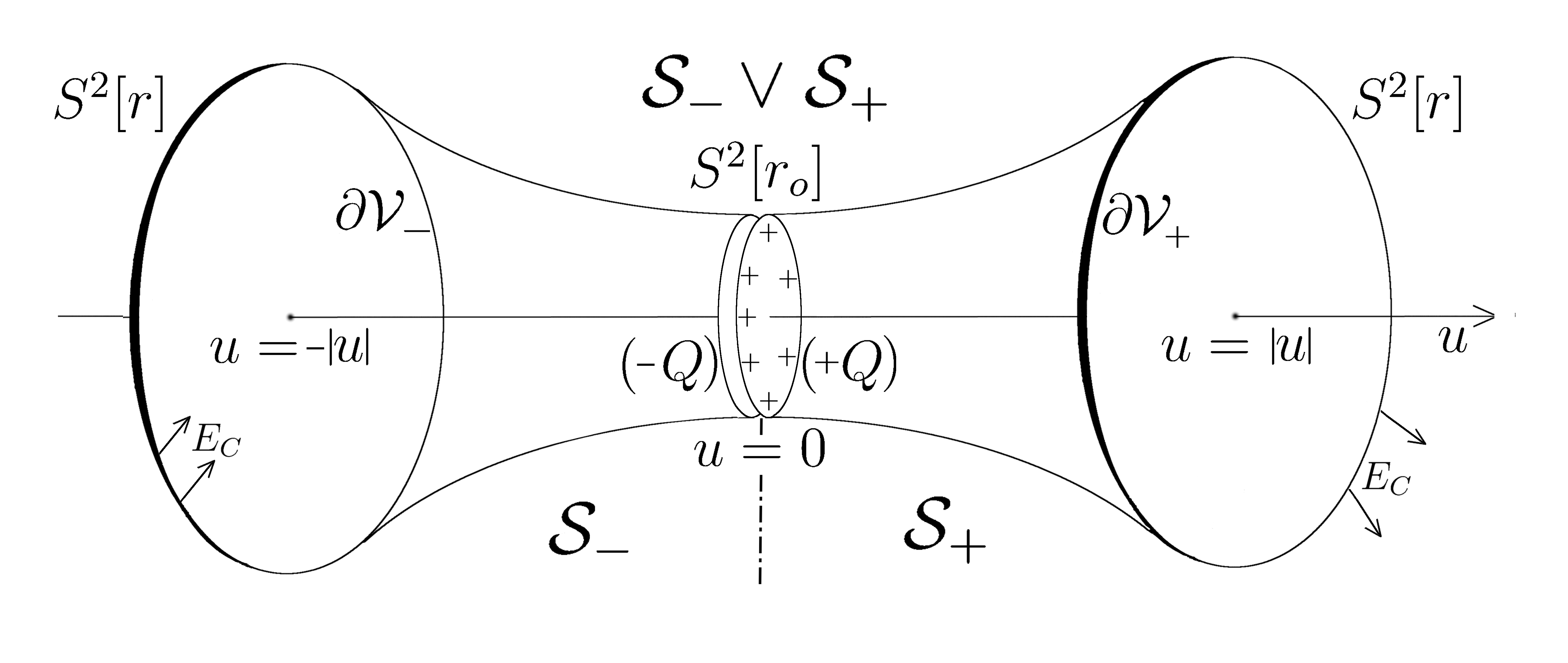
Figure 2: Round $S^{2}[r]$ sections along the $r=\pm{\rm L_{o}}\sqrt{P}u$ null-cone as (not shown) asymptote. (i) Disconnected $\partial{\cal V}_{\pm}$ boundary of $du=0$ hypersurface ${\cal V}$ in ${\cal G}$. (ii) Via $S^{2}[r_{o}]$ and $S^{2}[r]$ on the right in ${\cal S_{+}}$ it is established that ‘${\cal G}/2$’ $={\cal S}_{Q}$ carries actual $Q$ charge on the $S^{2}[r_{o}]$ of $\partial{\cal S}_{Q}$.

As usual, we can let $\partial{\cal V}$ surround the origin, which, instead of an “$r=0$ point”, is the $u=0$ locus, namely the small $S^{2}[r_{o}]$ sphere shown in Fig.2. By $\partial{\cal G}=0$ and the fact that such $u\!=$constant slices in ${\cal G}$ receive legitimate contributions from both of ${\cal S_{\pm}}$, the $\partial{\cal V}$ of any $du=0$ volume ${\cal V}$ must be a disconnected set. This is actually shown in Fig.2 as the ${\partial{\cal V_{\pm}}}$ pair of round-$S^{2}[r]$, which approach asymptotically the (not shown) null cone given as $r=\sqrt{P}{\rm L_{o}}|u|$ in (2.11). To better visualize this null cone, one could draw (mentally or actually) in Fig.2 the $\pm{\rm L_{o}}\sqrt{P}u$ asymptotes from diagram (i) of Fig.1. Integrating the electric flux ($\ast F$) through these $S^{2}[r]$ round spheres we find

$$0=\int_{\cal V}\!d\ast F=\int_{\partial{\cal V}}\!\ast F=\int_{\partial{\cal V_{+}}}\!\!\ast F+\int_{\partial{\cal V_{-}}}\!\!\ast F=\left[4\pi Q\right]_{\cal S_{+}}+\left[-4\pi Q\right]_{\cal S_{-}},$$ (3.12)

where the minus sign comes from ${\partial{\cal V_{-}}}$ in the (moving backwards in time) ${\cal S_{-}}$, so the overall null result is upheld. This leaves no actual $Q$ to be trapped in any ${\cal V}$ in ${\cal S_{-}}\!\vee{\cal S_{+}}$; the flux is not interrupted through any $S^{2}$ section, notably through $S^{2}[r_{o}]$, so $E_{C}$ is indeed a primordial field in ${\cal G}$. By the $\ast F\rightarrow F$ symmetry applied to (3.12), $B_{C}=Q/r^{2}$ is likewise established as a primordial magnetic field, so there can be no actual magnetic charge $Q$ or Dirac-string singularities in any ${\cal G}$-geon monopole. The smoothness of potential and fields in (3.11) cannot inhibit the emergence of Dirac’s quantization condition. To see that explicitly, we turn to the $A^{\rm(m)}$ potentials in (3.11) for a pair of $A^{\rm(m)}_{\;\;\pm}$, to cover (as atlas with an equatorial overlap) any given enclosing round-$S^{2}$, e.g., any typical $S^{2}[r]$ in Fig.2. In our case, as with the Dirac-monopole, exactly the same $2\pi n$ ($n\!\in\!Z$) phase difference will be recovered in the mentioned $A^{\rm(m)}_{\;\;+}\cap A^{\rm(m)}_{\;\;-}$ overlap in ${\cal G}$. And likewise for the ${\cal S}_{Q}$ geon, examined next.

4 Topological confinement of actual charges on $\partial{\cal S}_{Q}$

The concept of ${\cal S}_{Q}$ is referred-to as ${\cal G}/2$ because it emerged from ${\cal G}={\cal S_{-}}\!\vee{\cal S_{+}}$ when the $C^{\infty}$ junction across $S^{2}[r_{o}]$ at $u=0$ was undone (severed), leaving behind a null squashed-$S^{3}$ boundary $\partial{\cal S}_{Q}\neq 0$ as a physical singularity. As previewed, the new initial-value problem involves em field-lines terminating on the round-$S^{2}[r_{o}]$ section of $\partial{\cal S}_{Q}$, thus revealing actual electric (or magnetic) charge $Q$, trapped by topology and distributed homogeneously on $S^{2}[r_{o}]$ as surface-charge density $\sigma_{Q}$. To prove this, we can employ the divergence theorem with $\sigma_{Q}$ as an “almost point charge” surrounded by any $S^{2}[r]$ as a Gauss sphere in Fig.2. All incomplete geodesics also end on $\partial{\cal S}_{Q}$, so the gravitational initial-value problem likewise uncovers the presence of actual mass density $\rho_{m_{S}}$ on $S^{2}[r_{o}]$. This will integrate to $m_{S}$ (cf., next section), a mass-charge viewable as bare mass of ${\cal S}_{Q}$, in full analogy to the $Q$-charge from $\sigma_{Q}$. The total mass of ${\cal S}_{Q}$ will be $2m_{S}$, when we also include effective contributions from the energy density of the surrounding gravitational and em fields, supplying an additional $m_{S}$ input. Collecting these results, with $\rho_{Q}$ defined by analogy to $\rho_{m_{S}}$, we have

$$\rho_{Q}=\sigma_{Q}\,\delta(r-r_{o})=\frac{Q}{4\pi r^{2}}\,\delta(r-r_{o}),\;\;\;\rho_{m_{S}}=\frac{m_{S}}{4\pi r^{2}}\,\delta(r-r_{o}),\;\;\;\rho_{\rm em}=\frac{Q^{2}/r_{o}}{4\pi r^{2}}\,\delta(r-r_{o}),$$ (4.1)

where $Q^{2}/r_{o}$ is the em potential self-energy of $\sigma_{Q}$, confined as it is on $S^{2}[r_{o}]$. By the concept of any initial-value problem, subsequent sections of ${\cal S}_{Q}$, propagating beyond the ‘initial’ ${\partial\cal S}_{Q}$, will be totally ‘unaware’ whether any detachment has taken place at that ${\partial\cal S}_{Q}$. Thus, an overall stress-energy distribution $\tau_{\alpha\beta}$ must carry the full content of (4.1) plus (not shown) contributions from higher moments, etc, in a total energy-momentum distribution

$$T_{\alpha\beta}=\tau_{\alpha\beta}\,\delta(r-r_{o})\,.$$ (4.2)

$T_{\alpha\beta}$, quite distinct from $T_{\alpha\beta}^{\rm({\sc em})}$ in (2.8), involves all mentioned or implied contributions from charges on $S^{2}[r_{o}]$, namely electric (or magnetic) $Q$-charge and higher moments, $m_{S}$ bare mass, $\kappa Q=2r_{o}$ diameter, spin, gravitational and em self-energy, etc. These are confined as ‘quantum numbers’ on the round $S^{2}[r_{o}]$, which remains their host at $r=r_{o}$ even if the initial-value problem is set on subsequent $S^{2}[r]$ sections beyond ${\partial\cal S}_{Q}$: in spite of accordingly large $r>r_{o}$ radii in $(L_{1})^{2}=(L_{2})^{2}=r^{2}$ (cf., Fig.2), the $(L_{3})^{2}=-(2r_{o})^{2}$ value remains elementary, as a basic aspect of topological confinement on $S^{2}[r_{o}]$ shared by the general squashed-$S^{3}$ in ${\cal S}_{Q}$. This could also relate to stability, as conjectured in the next section.

5 On asymptotic infinity, causality, and stability of ${\cal G}$

All four ${\cal G}$,${\cal S}_{Q}$,$\bar{\cal G}$,$\bar{\cal S}_{Q}$ geons and (defined by time-reversal) antigeons are asymptotically locally flat manifolds at $r\rightarrow r_{\rm cl}$. The $r\rightarrow r_{o}$ limit is also objective and physical, because it relates to violations of causality via (5.3), as we’ll see. Vorticity is defined as

$$\omega:=\ast(v\wedge dv)=\frac{2r_{o}}{r^{2}}\,\theta^{3}\,,$$ (5.1)

calculated here for an observer with 4-velocity $V$, dual of $v=dt+{\rm L_{o}}/{\sqrt{P}}\cos\theta d\phi$ from (2.12). As seen in Fig.1, asymptotic infinity is actually realized when $r$ has practically fallen on the $+{\rm L_{o}}\sqrt{P}|u|$ asymptote in (2.11). There, by (3.4) etc, $R^{\mu}_{\;\nu\rho\sigma}$ vanishes at least as O$(r^{-2})$, with $W^{\alpha}_{\;\beta\gamma\delta}\sim r^{-3}$. This means that ${\cal G}$,${\cal S}_{Q}$,$\bar{\cal G}$,$\bar{\cal S}_{Q}$ could carry spin ${\sf s}_{G}$, effective mass $m_{G}$, and other charges, if found to be well-defined and finite ‘quantum numbers’, as mentioned. They will then be shared (up to $Q/|Q|$ signs) by ${\cal G}$,${\cal S}_{Q}$,$\bar{\cal G}$,$\bar{\cal S}_{Q}$, because all-four share the same asymptotic infinity. To see that this is actually the case here, and aiming to the upcoming (5.4), we introduce holonomic $x^{i}$ coordinates and global $t$-time from (2.13) via (2.11) as

$$x^{\mu}=(x^{0},x^{i}),\;\;\;\;\;x^{0}=t={\rm L_{o}}{\sqrt{P}}u+2r_{o}\psi=\pm\sqrt{r^{2}-r_{o}^{2}}+2r_{o}\psi\;\;\;\;\left[\psi\,{\rm mod}\;4\pi n\right].$$ (5.2)

The $8\pi nr_{o}$ $(n\!\in\!Z)$ homotopy-group structure from the $\psi\in[0,4\pi)$ angle in the timelike dimension of $S^{3}$ is mandatory, so any timelike direction in ${\cal G}$ can hardly avoid the involvement of the presence of $\psi$ and the causality-violating $t$-time loops it allows. This potentially disastrous result, which also exists in Taub-NUT, can here be naturally confined within sufficiently small $r\geq r_{o}$ radii. These, even when enormous w.r.t. Planck length, can and must remain elementary. Accordingly, classical causality is protected if the first bound in

$$r>r_{\rm sm}\geq r_{o}\;\;\;\;\;\;\left[|Q|\leq\frac{r_{\rm sm}}{\kappa}\right],\;\;\;\;\;\;\;\;\;m_{G}\geq\frac{|Q|}{\kappa}\;\longrightarrow\;\;\;P\leq 8\pi^{4}$$ (5.3)

can be observed [under a generally imposed constraint on the $Q$ parameter]. The second, a Bogomol’nyi bound as it applies in our case [10], has been evaluated in terms of the effective $m_{G}$ from em energy density via the upcoming (5.6); it has been equivalently expressed as an upper bound for the $P$ parameter. At $r\approx r_{o}$ scales, this Bogomol’nyi bound will be the only constraint applicable so close to the Big Bang. There, the first bound in (5.3) is violated for as long as the $2r_{o}\psi$ term in (5.2) dominates over the (normally enormous) ${\rm L_{o}}\sqrt{P}u$ term, as we’ll see. Sufficiently beyond the $r\approx r_{o}$ region, with $t$ turning null as $t\sim u$, classical causality is protected and (2.10) holds for $t$ as well. At $r>>r_{o}$, manifest general covariance in ${\cal G}$ can be traded for the standard $\eta_{\mu\nu}+h_{\mu\nu}$ perturbation in Minkowski’s $M_{\!o}^{4}$, so, at asymptotic infinity (if it acceptably exists, with $h_{\mu\nu}\rightarrow 0$ as $r\rightarrow\infty$), $M_{\!o}^{4}$ is elevated to a $M^{4}\approx{\cal G}$. Remarkably, here we can actually have $M^{4}={\cal G}$ exactly. Indeed, by (5.2) etc, we can re-express (2.12) in such $\eta_{\mu\nu}+h_{\mu\nu}$ form in terms of $(t,r,\theta,\phi)$ coordinates as

$$ds^{2}=\eta_{\mu\nu}dx^{\mu}dx^{\nu}+\frac{r_{o}^{2}}{r^{2}-r_{o}^{2}}(dr)^{2}-4r_{o}\cos\theta d\phi\left(dt+r_{o}\cos\theta d\phi\right),$$ (5.4)

to read-off all $h_{\mu\nu}$, scaled as they are by $\kappa Q=2r_{o}$. Thus , in addition to fixing the strength of the em content, the NUT-like charge also determines where the gravitational asymptotic infinity has actually been realized. Accordingly, the formal $r\rightarrow\infty$ limit can (and it will) be safely replaced by an earlier one, e.g., the $r\rightarrow r_{\rm sm}$ in the 4-scale hierarchy in (2.16). The price for these deeper findings has been the loss of manifest left-$SU(2)$ invariance, due to the absorption of $\psi$ in the definition of $t$ back in (2.13), here realized as the survival of $\theta,\phi$ in (5.4). This could (and here it does) hinder the calculation of mass and spin [11] (p.165 ff). Accordingly, we have to resort to estimates. Thus, to evaluate the Bogomol’nyi bound in (5.3), we assume that $m_{G}=2m_{S}$ comes solely from em energy density. Integrating $T_{00}^{\rm(em)}$ between $r_{o}$ ($u=0$) and $r$, with volume element $\theta^{1}\wedge\theta^{2}\wedge\theta^{3}$, we find a finite $m_{S}$ value

$$m(r)=\pi Q^{2}\sqrt{\frac{2}{P}}\int_{r_{o}}^{r}\frac{d\sqrt{r^{2}-r_{o}^{2}}}{r^{2}}\;+O(r^{-2})\,\;\;\stackrel{{\scriptstyle r\rightarrow\infty}}{{\longrightarrow}}\;\;\;\;m_{S}=\frac{\pi^{2}Q^{2}}{\sqrt{2P}r_{o}},$$ (5.5)

at the formal $r\rightarrow\infty$ limit. Practically, this $m_{S}$ value (and asymptotic infinity as $h_{\mu\nu}\rightarrow 0$) has been already reached at much-earlier limits, e.g., the $r\rightarrow r_{\rm sm}$ in the case of a 4-scale hierarchy in (2.16). We also note that, had the geometry allowed the $r_{o}=0$ value, the $r\rightarrow\infty$ limit in (5.5) would have simply reproduced the notorious (and here disastrous) result of a diverging $m_{S}$. By integrating over $u\in(-\infty,+\infty)$ in (5.5) to cover the entire ${\cal G}$ manifold (and likewise with $\omega r^{2}dm$ as angular momentum element), we find

$$r\longrightarrow r_{\rm sm}\;\;\left(h_{\mu\nu}\longrightarrow 0\right):\;\;\;\;\;\;\;\;\;\;m_{G}=2m_{S}\approx\frac{2\sqrt{2}\pi^{2}Q^{2}}{\rm L_{o}}\,,\;\;\;\;\;{\sf s}_{G}\sim\frac{2\sqrt{2}\pi^{2}Q^{2}}{\sqrt{P}}\,,$$ (5.6)

etc, where (5.1) has also been used to estimate spin. We recall that these results are shared as ‘quantum numbers’ by all four ${\cal G}$,$\bar{\cal G}$,${\cal S}_{Q}$,$\bar{\cal S}_{Q}$, up to a $Q/|Q|$ sign and particular aspects. An example of the latter is the $2m_{S}$ value as mass of ${\cal S}_{Q}$, realized as the sum of $m_{S}$ as the bare mass in (4.1), plus the em contribution (an additional $m_{S}$) from integrating over a single covering of ${\cal S}_{Q}$, actually as calculated in (5.5).

There exists no interaction between the ${\cal S_{\pm}}$ constituents of ${\cal G}={\cal S_{-}}\vee{\cal S_{+}}$, hence neither a relation to $\bar{p}p$ (positronium-like) states, which are typically unstable. A plausible and in agreement with observation (but only comparative) statement on the stability of the ${\cal G}$ geon is that the magnetic (3.11) types are favored vs the electric (3.10), as the former have very few or virtually no channels to decompose into conventional magnetic monopoles or disperse into magnetic vortices. The confinement of actual charge on $S^{2}[r_{o}]$ could relate to the stability of ${\cal S}_{Q}$, if the latter could be viewed as an equilibrium state between gravitational collapse within $S^{2}[r_{o}]$ and the outburst of $\sigma_{Q}$ off $S^{2}[r_{o}]$ as no-go extremes. Similar approaches do exist, but they are all tentative prior to a needed rigorous study. In any case, any issue or result on the stability of ${\cal G}$ would also illuminate the likewise suspended issue on the stability of the Kerr-Newman solution, which has been fundamentally upgraded by ${\cal S}_{Q}$ .

6 Conclusions

1. We have examined the strong similarities and the even stronger differences between the ${\cal G}$-geon vs the Taub-NUT. Sections 4,5 also allow a comparison between the ${\cal S}_{Q}$-geon and the Kerr-Newman solution, with the content of the former being richer (with higher em moments, in addition to spin, mass, etc) and more predictive. ${\cal S}_{Q}$ is also non-singular, regardless of hierarchy type in (2.16), as any geon must be by concept. The admittance of any spacetime singularity sufficiently close to the Big-Bang would redirect the latter’s dynamics (one of a time-reversed black hole) toward that of the added singularity, so as to produce a loop of failed or aborted Big-Bang, roughly as a wormhole with its open regions topologically identified. ${\cal G}$,${\cal S}_{Q}$,$\bar{\cal G}$,$\bar{\cal S}_{Q}$, referred-to collectively as ${\cal G}$ unless explicitly distinguished, share the same asymptotic infinity, hence the same spin, mass, etc, up to $Q/|Q|$ signs. They also admit the presence of a sufficiently weak scalar field in a 3-parameter generalization.

2. ${\cal G}$ geons admit timelike loops, bifurcating geodesics, etc, but, as a fifth fundamental difference vs Taub-NUT, the natural confinement of such non-classical dynamics has been possible within the bounds described by the first inequality in (5.3). Whenever the latter can be observed, accordingly-enforced is the protection of classical causality. The violation of the first constraint in (5.3), hence of causality, is of course an important aspect of the quantum regime. Here however, this violation acquires additional importance for models close to the Big-Bang, as with the ${\cal G}_{\rm bb}$ geon (cf., paragraph 5 below).

3. The constraints in (5.3) are well-defined in ${\cal G}$, but, particularly the Bogomol’nyi bound, cannot be really applied to the Taub-NUT vacuum. Expressed as upper-bounds on $P,Q$ in (5.3), they also shape as accordingly-constrained the $(P,Q)$ parameter space of ${\cal G}$. With no constraints, this space would involve any $P>0$, $Q\neq 0$ value, with (i) $Q$ fixing $2r_{o}=\kappa|Q|$, hence the asymptotic infinity for gravity and the strength of the em content (effective or actual), and (ii) $P/Q^{2}$ providing independent scaling of the $m_{G}$ mass in units of $\kappa$. The constraints in (5.3) are also expected to incite predictions, as it actually happens in the following previews on anticipated ${\cal G}$-geon dynamics.

4. The main idea and approach is to describe and study this dynamics in terms of analytic simulations (discreetly distanced from controversial HEP considerations), in Friedman-like evolution models ${\cal F}$, one per case, such as the ${\cal F}_{o}$ and ${\cal F}^{\prime}_{o}$ (outlined next) or the ${\cal F}_{\rm bb}$ (outlined last). To begin with the simplest non-trivial example, (i) ${\cal F}_{o}$ is filled with ${\cal G}_{o}$ geons, hardly interacting to simulate dark-matter dust. The $r_{\rm cl}$ radius in (2.16) can be exploited here as a third parameter, so the $P,Q$ can be spent to restrain mass and $Q$-charge of the DM particle within bounds compatible with data from HEP and cosmology. Then, spin, dipole and quadrapole moments, as well as the dating of ${\cal G}_{o}$ in early afterglow in a 4-scale hierarchy (2.16), would then be predictions of the model. (ii) ${\cal F}^{\prime}_{o}$ is also filled with ${\cal G}_{o}$ geons, now mixed randomly with ${\cal G}^{\prime}_{o}$ geons which are fewer but have much larger $Q^{\prime}$,$m^{\prime}_{G}$ values compared to those of ${\cal G}_{o}$. Having $P^{\prime}$,$Q^{\prime}$ values in a 3-scale hierarchy in (2.16), the ${\cal G}^{\prime}_{o}$ as seed particles will expectedly shape the dynamics in ${\cal F}^{\prime}_{o}$ as one of accretion, trapping DM particles plus baryons (if also present in the model). A primordial stability-enhancing magnetic field is actually predicted as $B^{\prime}_{C}=Q^{\prime}/{r^{\prime}_{\rm cl}}^{\!2}$ at the time this pre-galactic dynamics commences (near recombination, around the end of the so-called dark ages).

5. The ${\cal F}_{\rm bb}$ model could involve many or just one ‘cosmogonic’ ${\cal G}_{\rm bb}$ geon in a 4-scale hierarchy in (2.16), and an (even sub-Planck) $2r_{o}$ size. ${\cal G}_{\rm bb}$ could provide analytic simulations of primordial gravitational waves, created with the first quantum fluctuation(s) of the vacuum. These configurations are highly non-linear and must be in agreement with the Bogomol’nyi bound in (5.3), hence with possibly enormous ‘mass-energy’. At the same time, the first bound in (5.3) must be violated for as long as $t$ in (5.2) is sufficiently close to $t=0$, or, equivalently, $r$ is extremely near $r_{o}$. There, large $n>1$ values are allowed and they could even be induced in repeatedly circling time-loops, feeding superluminal expansion and global violation of causality, in exact models for analytic simulations of inflationary dynamics. This dynamics, with amplifications etc, is expected to last for as long as the $2r_{o}\psi$ term retains its dominance over the $\sqrt{r^{2}-r_{o}^{2}}$ term in (5.2). When that dominance is reversed by sufficiently large $r$, the first bound in (5.3) is realized as applicable for the first time, inflation stops, and an expanding causal classical regime is born. The ${\cal G}_{\rm bb}$ geon(s), created shortly after the Big Bang and amplified during inflation, are expected to reach asymptotic infinity somewhere within the afterglow era. As a general result, the ${\cal G}_{o}$,${\cal G}^{\prime}_{o}$,${\cal G}_{\rm bb}$ examples also serve as paradigms of gravity giving $2r_{o}$ size from NUT-like charge, and independently-scaled mass (or pp-wave energy) to particle-like configurations. Those previewed here, as well as other ${\cal G}$ or ${\cal S}_{Q}$ geon configurations, may provide analytic models with current observational and novel theoretical interest in particle physics and cosmology.

The author is grateful to A.A. Kehagias for discussions.

References

- [1] A. Einstein, L. Infeld, B. Hoffmann, Ann. of Math. (2nd series) 39 (1938) 65-100; A. Einstein and W. Pauli, Ann. Math. 44 (1943) 131; A. Papapetrou, Ann. Physik. 9 (1962) 97.
- [2] É. Cartan, La théorie des groupes finis et continus et la géométrie différentielle traitées par la méthode du repére mobile (Gauthier-Villars, Paris 1937).
-
[3]
A. Lichnerowicz, Théories Relativiste de la Gravitation et de l’Électromagnétisme
(Masson, Paris, 1955). - [4] J.A. Wheeler, Phys.Rev. 97 (1957) 511.
- [5] A.H. Taub, An. Math. 53 (1951) 472; E. Newman, L. Tamburino, T. Unti, J. Math. Phys. 4 (1963) 915; C.W. Misner, J. Math. Phys. 4 (1963) 924; C.W. Misner and A.H. Taub (1968), Engl. Transl. Sov. Phys.-JETP 28 (1969) 122.
- [6] M. Ryan and L. Shepley, Homogeneous Relativistic Cosmologies (PUP, N.J., 1975); T. Eguchi. P.B. Gilkey, A.J. Hanson, Phys.Rep. 66 (1980) 213-393; M.J. Duff, B.E.W. Nilsson, C.N. Pope, Phys. Rep. 130 (1986) 1.
-
[7]
J.P. Griffiths and J. Podolsky, Exact space-times in Einstein’s General Relativity
(Cambridge Monographs on Mathematical Physics, Cambridge 2010). - [8] D.R. Brill and J.B. Hartle, Phys.Rev. 135 (1964) B271; P.R. Anderson and D.R. Brill Phys.Rev.D 56 (1997) 4824.
- [9] R.D. Sorkin, Introduction to topological geons (Erice, Italy, 1985); J. Louko, J. Phys.: Conf. Ser. 222 012038 (2010).
- [10] G.W. Gibbons and C.M. Hull, Phys. Lett. B 199 (1982) 190.
- [11] S. Weinberg, Gravitation and Cosmology (Wiley, New York, 1972).