Admissible Invariants of genus 3 Curves

Abstract.

Several invariants of polarized metrized graphs and their applications in Arithmetic Geometry are studied recently. In this paper, we explicitly calculated these admissible invariants for all curves of genus $3$. We find the sharp lower bound for the invariants $\varphi$, $\lambda$ and $\epsilon$ for all polarized metrized graphs of genus $3$. This improves the lower bound given for Effective Bogomolov Conjecture for such curves.

1. Introduction

Invariants of a polarized metrized graph $(\Gamma,\textbf{q})$ are of interest for more than last twenty years because of their applications in arithmetic geometry and number theory. The invariants $\varphi(\Gamma)$, $\lambda(\Gamma)$ and $\epsilon(\Gamma)$, see below for their definitions, are studied for their connection to the self intersection of admissible dualizing sheaf associated to a curve of genus at least $2$ over a global field. One can consult to S. Zhang’s articles [21] and [22] for technical details. On the other hand, L. Szpiro showed in [16] and [17] that both Bogomolov and Effective Mordell conjectures can be stated as ‘suitable’ upper and lower bounds to self intersection of certain dualizing sheaf.

Lower bounds for $\varphi(\Gamma)$, $\lambda(\Gamma)$ are given in [6, Theorems 2.11 and 2.13] for all curves of genus greater than $1$. However, obtaining sharp bounds and explicit computations for each possible case were done for only certain type of curves. For curves of small genus, the invariants $\varphi(\Gamma)$, $\lambda(\Gamma)$ and $\epsilon(\Gamma)$ are studied in [14], [15], [18], [20], [11], [10]. It will be of reader’s interest to see [12], [13] and [19], too.

When $(\Gamma,\textbf{q})$ has genus $2$, A. Moriwaki computed several invariants including $\epsilon(\Gamma)$ for each case and obtained certain bound equivalent to the sharp lower bound $\varphi(\Gamma)\geq\frac{1}{27}\ell(\Gamma)$, where $\ell(\Gamma)$ is the total length of $\Gamma$. This bound is verified with different methods by X. Faber in [10] and the author in [6]. For a such $\Gamma$, Moriwaki in [15] and Jong in [11] explicitly computed these invariants for each genus $2$ curves. Jong’s work also extends to archimedean case, which is essential for number theoretic applications.

When $(\Gamma,\textbf{q})$ has genus $3$, K. Yamaki in [20], Faber in [10] and the author in [6] studied these invariants. Moreover, Faber showed [10, Theorem 3.4] that $\varphi(\Gamma)\geq c\delta_{0}(\Gamma)+\frac{4}{3}\delta_{1}(\Gamma)$ with $c=\frac{2}{81}$. Later, the author in [6, Theorem 2.11] improved this result by showing that $c$ can be taken as $\frac{1}{39}$. However, these lower bounds are not sharp.

Contributions of this paper are as follows:

(i) We determine all polarized metrized graphs $(\Gamma,\textbf{q})$ of genus $3$.

(ii) We explicitly compute various invariants including $\varphi(\Gamma)$, $\epsilon(\Gamma)$ and $\lambda(\Gamma)$ of all $(\Gamma,\textbf{q})$ of genus $3$.

(iii) We give sharp lower bounds for each of $\varphi(\Gamma)$, $\epsilon(\Gamma)$ and $\lambda(\Gamma)$. Namely, we show that if $(\Gamma,\textbf{q})$ is of genus $3$ and of total length $\ell(\Gamma)$, then $\varphi(\Gamma)\geq\frac{17}{288}\ell(\Gamma)$, $\lambda(\Gamma)\geq\frac{3}{28}\ell(\Gamma)$ and $\epsilon(\Gamma)\geq\frac{2}{9}\ell(\Gamma)$. As a result, via Zhang’s work, this improves the bound given for Effective Bogomolov Conjecture for genus $3$ case (see [6, Theorems 2.3 and 2.4]). Note that the bound $\frac{17}{288}\ell(\Gamma)$ for $\varphi(\Gamma)$ was conjectured by X. Faber in [10, Remark 5.1]. This lower bound is attained when $\Gamma$ is a regular tetrahedral graph. We note that the number $288$ also appears in Tartaglia’s formula for the volume of a tetrahedron, which is a generalization of Heron’s formula for the area of a triangle.

(iv) We obtain, as a by product, a highly nontrivial inequality that holds for any nonnegative six real numbers (see inequalities (7), (9) and (6) below). Interestingly, the terms that appear in these inequality corresponds to certain cycles of a tetrahedral graph which is not necessarily in ${\mathbb{R}}^{3}$.

2. pm-graphs and their invariants

In this section, we first give brief descriptions of a metrized graph $\Gamma$, a polarized metrized graph $(\Gamma,\textbf{q})$, invariants $\tau(\Gamma)$, $\theta(\Gamma)$, $\epsilon(\Gamma)$, $\varphi(\Gamma)$, $\lambda(\Gamma)$ and $Z(\Gamma)$ associated to $(\Gamma,\textbf{q})$.

A metrized graph $\Gamma$ is a finite connected graph equipped with a distinguished parametrization of each of its edges. A metrized graph $\Gamma$ can have multiple edges and self-loops. For any given $p\in\Gamma$, the number $\upsilon(p)$ of directions emanating from $p$ will be called the valence of $p$. By definition, there can be only finitely many $p\in\Gamma$ with $\upsilon(p)\not=2$.

For a metrized graph $\Gamma$, we will denote a vertex set for $\Gamma$ by $V(\Gamma)$. We require that $V(\Gamma)$ be finite and non-empty and that $p\in V(\Gamma)$ for each $p\in\Gamma$ if $\upsilon(p)\not=2$. For a given metrized graph $\Gamma$, it is possible to enlarge the vertex set $V(\Gamma)$ by considering additional valence $2$ points as vertices.

For a given metrized graph $\Gamma$ with vertex set $V(\Gamma)$, the set of edges of $\Gamma$ is the set of closed line segments with end points in $V(\Gamma)$. We will denote the set of edges of $\Gamma$ by $E(\Gamma)$. However, if $e_{i}$ is an edge, by $\Gamma-e_{i}$ we mean the graph obtained by deleting the interior of $e_{i}$.

We define the genus of $\Gamma$ to be the first Betti number $g(\Gamma):=e-v+1$ of the graph $\Gamma$, where $e$ and $v$ are the number of edges and vertices of $\Gamma$, respectively.

Length of an edge of $\Gamma$ is a positive real number. If we denote the length of an edge $e_{i}\in E(\Gamma)$ by $L_{i}$, the total length of $\Gamma$, which is denoted by $\ell(\Gamma)$, is given by $\ell(\Gamma)=\sum_{i=1}^{e}L_{i}$.

The tau constant $\tau(\Gamma)$ of a metrized graph $\Gamma$ was initially defined by Baker and Rumely in [2, Section 14]. The following lemma gives a description of the tau constant. In particular, it implies that the tau constant is positive.

Lemma 2.1.

[2, Lemma 14.4] Let $r(x,y)$ be the resistance function on $\Gamma$. For any fixed $y$ in $\Gamma$, $\tau(\Gamma)=\frac{1}{4}\int_{\Gamma}\big{(}\frac{\partial}{\partial x}r(x,y)\big{)}^{2}dx$.

One can find more detailed information on $\tau(\Gamma)$ in articles [3], [4], [5] and [7]. For more information about the resistance function $r(x,y)$ on a metrized graph, one can consult to the articles [2], [1] and [4].

Let $\Gamma$ be a metrized graph with a vertex set $V(\Gamma)$, and let $\textbf{q}:\Gamma\rightarrow{\mathbb{N}}$ be a function supported on a subset of $V(\Gamma)$. That is, $\textbf{q}(s)=0$ for all $s\in\Gamma-V(\Gamma)$, and whenever $\textbf{q}(s)>0$ we must have $s\in V(\Gamma)$.

A divisor on $\Gamma$ is a formal sum $\sum n_{i}p_{i}$, where $a_{i}\in{\mathbb{Z}}$ and $p_{i}\in\Gamma$ for every $i$. A divisor $\sum n_{i}p_{i}$ on $\Gamma$ is called effective if $n_{i}\geq 0$ for all $i$.

The canonical divisor $K$ of $(\Gamma,\textbf{q})$ is defined as follows:

(1) $$\begin{split}K=\sum_{p\in V(\Gamma)}(\upsilon(p)-2+2\textbf{q}(p))p.\end{split}$$

The pair $(\Gamma,\textbf{q})$ is called a polarized metrized graph (pm-graph in short) if $K$ is an effective divisor. Whenever $\textbf{q}=0$, $(\Gamma,\textbf{q})$ is called a simple pm-graph. We define the genus $\bar{g}(\Gamma)$ of a pm-graph $(\Gamma,\textbf{q})$ as follows:

(2) $$\begin{split}\bar{g}(\Gamma)=g(\Gamma)+\sum_{p\in V(\Gamma)}\textbf{q}(p).\end{split}$$

If $\Gamma$ under consideration is clear, we simply use notations $g$ and $\bar{g}$ instead of $\bar{g}(\Gamma)$ and $g(\Gamma)$, respectively.

Remark 2.2.

For each $p\in V(\Gamma)$, $\upsilon(p)-2+2\textbf{q}(p)\geq 0$ and $\textbf{q}(p)\geq 0$, since the canonical divisor $K$ is effective and q is nonnegative. In particular, if $\upsilon(p)=1$ for some $p\in\Gamma$, we should have $p\in V(\Gamma)$ and $\textbf{q}(p)\geq 1$.

On a pm-graph $(\Gamma,\textbf{q})$, we defined and studied the invariant $\theta(\Gamma)$ in [3] and [6] as follows:

(3) $$\begin{split}\theta(\Gamma)=\sum_{p,\,q\in\,V(\Gamma)}(\upsilon(p)-2+2\textbf{q}(p))(\upsilon(q)-2+2\textbf{q}(q))r(p,q).\end{split}$$

We have $\theta(\Gamma)\geq 0$ for any pm-graph $\Gamma$, since the canonical divisor $K$ is effective.

Let $\mu_{ad}(x)$ be the admissible measure associated to $K$ (defined by Zhang [21, Lemma 3.7]). Next, we give definitions of the invariants $\epsilon(\Gamma)$, $\varphi(\Gamma)$, $\lambda(\Gamma)$ and $Z(\Gamma)$ (c.f. [22, Section 4.1]) of $\Gamma$:

(4) $$\epsilon(\Gamma) =\iint_{\Gamma\times\Gamma}r(x,y)\delta_{K}(x)\mu_{ad}(y), \quad Z(\Gamma) =\frac{1}{2}\iint_{\Gamma\times\Gamma}r(x,y)\mu_{ad}(x)\mu_{ad}(y),$$

$$\varphi(\Gamma) =3\bar{g}\cdot Z(\Gamma)-\frac{1}{4}(\epsilon(\Gamma)+\ell(\Gamma)), \quad\lambda(\Gamma) =\frac{\bar{g}-1}{6(2\bar{g}+1)}\varphi(\Gamma)+\frac{1}{12}(\epsilon(\Gamma)+\ell(\Gamma)).$$

We can express each invariant given in Equation (4) in terms of $\tau(\Gamma)$ and $\theta(\Gamma)$ ([6, Propositions 4.6, 4.7, 4.9 and Theorem 4.8]):

Theorem 2.3.

Let $(\Gamma,\textbf{q})$ be a pm-graph with $\bar{g}=3$. Then we have

$$\varphi(\Gamma) =\frac{13}{3}\tau(\Gamma)+\frac{\theta(\Gamma)}{12}-\frac{\ell(\Gamma)}{4}, Z(\Gamma) =\frac{5}{9}\tau(\Gamma)+\frac{\theta(\Gamma)}{72},$$

$$\lambda(\Gamma) =\frac{3}{7}\tau(\Gamma)+\frac{\theta(\Gamma)}{56}+\frac{\ell(\Gamma)}{14}, \epsilon(\Gamma) =\frac{8}{3}\tau(\Gamma)+\frac{\theta(\Gamma)}{6}.$$

Let $p$ be a point in a pm-graph $\Gamma$ such that $p\not\in V(\Gamma)$. That is, $p$ is not an end point of any edge in $E(\Gamma)$. Let $\Gamma$-${p}$ be the pm-graph obtained from $\Gamma$ by removing $p$ and adding two points $p_{1}$ and $p_{2}$ to make the remaining parts closed. That is, $\Gamma$ is obtained from $\Gamma$-$p$ by identifying the end points $p_{1}$ and $p_{2}$. Following Zhang’s definition [22, Section 4.1], we call $p$ is of type $0$ if $\Gamma$-${p}$ is connected. This happens when $p$ is contained in an edge such that removing the edge does not disconnect $\Gamma$. If $p$ is not of type $0$, $\Gamma$-${p}$ is a union of two connected metrized subgraphs with functions $\textbf{q}_{1}$ and $\textbf{q}_{2}$ that are restrictions of q and satisfy $\textbf{q}_{1}(p_{1})=\textbf{q}_{2}(p_{2})=0$. By applying Equation (2), we see that the subgraphs are of genus $i$ and $\bar{g}-i$ for some integer $i\in(0,\bar{g}/2]$. In this case, we call $p$ is of type $i$. For each integer $i\in[0,\bar{g}/2]$, let $\Gamma_{i}$ be the subgraph of $\Gamma$ of points of type $i$, and let $\ell_{i}(\Gamma)$ be the total length of $\Gamma_{i}$. We use the invariants $\delta_{i}(\Gamma):=\ell_{i}(\Gamma)$ for each $i\geq 0$ (see [6] or [22] for geometric meaning of these invariants). Therefore, whenever $\bar{g}=3$, we have only type $0$ and $1$ points, so we consider only the invariants $\delta_{0}(\Gamma)$ and $\delta_{1}(\Gamma)$ for which we have $\ell(\Gamma)=\delta_{0}(\Gamma)+\delta_{1}(\Gamma)$.

Remark 2.4.

Given a pm-graph $(\Gamma,\textbf{q})$ with a vertex set $V(\Gamma)$ containing at least two elements, suppose $\textbf{q}(s)=0$ and $\upsilon(s)=2$ for some $s\in V(\Gamma)$, then removing $s$ from the vertex set of $\Gamma$ does not change $\theta(\Gamma)$. Similarly, if a vertex $s$ is such that $\upsilon(s)=2$ and $V(\Gamma)-\{s\}$ has at least one element, then removing $s$ from $V(\Gamma)$ does not change $\tau(\Gamma)$. (such vertices are called eliminable vertices in [18, pg. 152]). We call these the valence property of $\tau(\Gamma)$ and $\theta(\Gamma)$, see [4, Remark 2.10]). Therefore, $\epsilon(\Gamma)$, $Z(\Gamma)$, $\varphi(\Gamma)$ and $\lambda(\Gamma)$ do not change under this process by Theorem 2.3. That is, each of these invariants has the valence property [8, Remark 2.4].

Remark 2.4 is very helpful to determine the possible pm-graphs of a given genus. As long as $V(\Gamma)$ is non-empty, it will be enough to consider pm-graphs not having any vertex $p$ with $\upsilon(p)=2$ and $\textbf{q}(p)=0$. In fact, in this way we choose only one model of a given pm-graph among all the equivalent models.

Recall that we consider only pm-graphs with $\bar{g}=3$ in this paper. Such pm-graphs can have any $g\in\{0,\,1,\,2,\,3\}$ by Equation (2). We designate a section for each such value of $g$ in the rest of the article. In each case, we first determine the pm-graphs with the desired $g$ and $\bar{g}$ up to equivalence. Then, we compute all the relevant invariants. Finally, we find sharp lower bounds to the invariants $\tau(\Gamma)$ and $\varphi(\Gamma)$, $\lambda(\Gamma)$ for all $\Gamma$ under consideration. We can use the techniques developed in [4] and [3] along with Theorem 2.3 to compute these invariants. This is what we did in this paper. Alternatively, we can compute these invariants by using the algorithms given in [7] and [8]. For example, how we compute the tau constant for the metrized graph in part $IX$ of Figure 4 is illustrated in [7, Example 5.2], and computation of invariants of the pm-graph in part $XIV$ of Figure 4 are done in [8, Example 1].

Note that we could consider only pm-graphs $XIII$ and $XIV$ in Figure 4 to obtain lower bound of $\varphi(\Gamma)$ for all pm-graphs of $\bar{g}=3$. The proof of this fact was given in [10, pages 360 and 365] (see also [6, pages 549 and 550]). Another approach utilizing this fact was also known to Yamaki (see [20, page 67] and [18, page 160]). However, our aim in this paper is more than finding the sharp lower bound, so we worked on all possible pm-graphs.

3. The case $g(\Gamma)=0$

Suppose $\Gamma$ is a pm-graph with $g(\Gamma)=0$ and $\bar{g}(\Gamma)=3$. Then Equation (2) becomes $3=\sum_{p\in V(\Gamma)}\textbf{q}(p)$. Moreover, it follows from Remark 2.2 that such a pm-graph can have at most three vertices with valence exactly $1$. On the other hand, $g(\Gamma)=0$ implies $e=v-1$.

If $\Gamma$ has no edges, then it is just a point $p$ with $\textbf{q}(p)=3$, as shown in part $I$ of Figure 1. Otherwise, pm-graphs $(\Gamma,\textbf{q})$ in this case are tree pm-graphs, which have at least two vertices with $\upsilon(p)=1$. Figure 1 illustrates the possible pm-graphs satisfying these conditions.

We have $\tau(\Gamma)=\frac{\ell(\Gamma)}{4}$ since $\Gamma$ is a metrized graph that is a tree graph [2, Equation 14.3], and we use Equation (3) to compute $\theta(\Gamma)$. Then we compute $\varphi(\Gamma)$, $\lambda(\Gamma)$ and $\epsilon(\Gamma)$ by using Theorem 2.3. The results are given in Table 1.

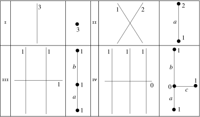
Figure 1. Irreducible components of genus 3 curves and their dual graphs when the dual graphs have genus $0$, i.e. when $\bar{g}=3$ and $g=0$.

	$\ell(\Gamma)$	$\delta_{0}(\Gamma)$	$\delta_{1}(\Gamma)$	$\tau(\Gamma)$	$\theta(\Gamma)$	$\varphi(\Gamma)$	$\lambda(\Gamma)$	$\epsilon(\Gamma)$
$I$	$0$	$0$	$0$	$0$	$0$	$0$	$0$	$0$
$II$	$a$	$0$	$\ell(\Gamma)$	$\frac{\ell(\Gamma)}{4}$	$6\ell(\Gamma)$	$\frac{4\ell(\Gamma)}{3}$	$\frac{2\ell(\Gamma)}{7}$	$\frac{5\ell(\Gamma)}{3}$
$III$	$a+b$	$0$	$\ell(\Gamma)$	$\frac{\ell(\Gamma)}{4}$	$6\ell(\Gamma)$	$\frac{4\ell(\Gamma)}{3}$	$\frac{2\ell(\Gamma)}{7}$	$\frac{5\ell(\Gamma)}{3}$
$IV$	$a+b+c$	$0$	$\ell(\Gamma)$	$\frac{\ell(\Gamma)}{4}$	$6\ell(\Gamma)$	$\frac{4\ell(\Gamma)}{3}$	$\frac{2\ell(\Gamma)}{7}$	$\frac{5\ell(\Gamma)}{3}$

Table 1. Pm-graph invariants when $g(\Gamma)=0$

We exclude the case $I$ in Table 1 as $\ell(\Gamma)=0$. In the other three cases, we have $\varphi(\Gamma)=\frac{4}{3}\ell(\Gamma)$, $\lambda(\Gamma)=\frac{2\ell(\Gamma)}{7}$ and $\epsilon(\Gamma)=\frac{5\ell(\Gamma)}{3}$.

4. The case $g(\Gamma)=1$

In this section, we consider pm-graphs $(\Gamma,\textbf{q})$ with $g=1$ and $\bar{g}=3$. It follows from Equation (2) that $2=\sum_{p\in V(\Gamma)}\textbf{q}(p)$. Thus, such a pm-graph can have at most two vertices with valence exactly $1$ by Remark 2.2. Since $g=1$, we have $e=v$. Based on these observations, Figure 2 illustrates the possible pm-graphs satisfying these conditions.

We have $\tau(\Gamma)=\frac{\ell(\Gamma)}{4}$ when $\Gamma$ is a tree metrized graph [2, Equation 14.3]. Moreover, $\tau(\Gamma)=\frac{\ell(\Gamma)}{12}$ when $\Gamma$ is a circle metrized graph [4, Corollary 2.17]. We use these facts and additive property of tau constant [4, page 15] to compute $\tau(\Gamma)$ for each pm-graphs listed in Figure 2. We again use Equation (3) to compute $\theta(\Gamma)$. Then we compute $\varphi(\Gamma)$, $\lambda(\Gamma)$ and $\epsilon(\Gamma)$ by using Theorem 2.3. The invariants $\delta_{0}(\Gamma)$ and $\delta_{1}(\Gamma)$ are determined by using their definitions and by considering the topology of $\Gamma$. The results are given in Table 2 and Table 3. As can be seen from Table 3, we have $\varphi(\Gamma)\geq\frac{1}{9}\ell(\Gamma)$, $\lambda(\Gamma)\geq\frac{3\ell(\Gamma)}{28}$, $\epsilon(\Gamma)\geq\frac{2\ell(\Gamma)}{9}$, and these lower bounds are attained by the pm-graph given in part $I$ of Figure 2.

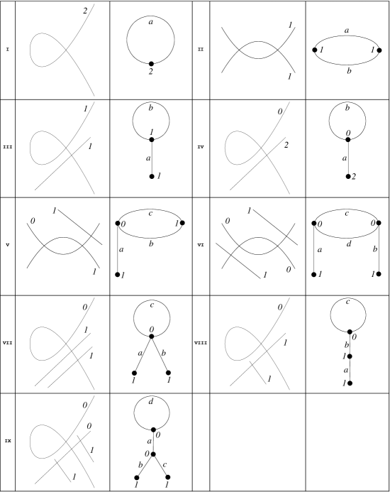
Figure 2. Irreducible components of genus 3 curves and their dual graphs when the dual graphs have genus $1$, i.e. when $\bar{g}=3$ and $g=1$.

	$\ell(\Gamma)$	$\delta_{0}(\Gamma)$	$\delta_{1}(\Gamma)$	$\tau(\Gamma)$	$\theta(\Gamma)$
$I$	$a$	$a$	$0$	$\frac{\ell(\Gamma)}{12}$	$0$
$II$	$a+b$	$a+b$	$0$	$\frac{\ell(\Gamma)}{12}$	$\frac{8ab}{a+b}$
$III$	$a+b$	$b$	$a$	$\frac{\ell(\Gamma)}{12}+\frac{a}{6}$	$6a$
$IV$	$a+b$	$b$	$a$	$\frac{\ell(\Gamma)}{12}+\frac{a}{6}$	$6a$
$V$	$a+b+c$	$b+c$	$a$	$\frac{\ell(\Gamma)}{12}+\frac{a}{6}$	$6a+\frac{8bc}{b+c}$
$VI$	$a+b+c+d$	$d+c$	$a+b$	$\frac{\ell(\Gamma)}{12}+\frac{a+b}{6}$	$6(a+b)+\frac{8cd}{c+d}$
$VII$	$a+b+c$	$c$	$a+b$	$\frac{\ell(\Gamma)}{12}+\frac{a+b}{6}$	$6(a+b)$
$VIII$	$a+b+c$	$c$	$a+b$	$\frac{\ell(\Gamma)}{12}+\frac{a+b}{6}$	$6(a+b)$
$IX$	$a+b+c+d$	$d$	$a+b+c$	$\frac{\ell(\Gamma)}{12}+\frac{a+b+c}{6}$	$6(a+b+c)$

Table 2. Pm-graph invariants when $g(\Gamma)=1$, part 1.

	$\varphi(\Gamma)$	$\lambda(\Gamma)$	$\epsilon(\Gamma)$
$I$	$\frac{\ell(\Gamma)}{9}$	$\frac{3\ell(\Gamma)}{28}$	$\frac{2\ell(\Gamma)}{9}$
$II$	$\frac{\ell(\Gamma)}{9}+\frac{2ab}{3(a+b)}$	$\frac{3\ell(\Gamma)}{28}+\frac{ab}{7(a+b)}$	$\frac{2\ell(\Gamma)}{9}+\frac{4ab}{3(a+b)}$
$III$	$\frac{\ell(\Gamma)}{9}+\frac{11a}{9}$	$\frac{3\ell(\Gamma)}{28}+\frac{5a}{28}$	$\frac{2\ell(\Gamma)}{9}+\frac{13a}{9}$
$IV$	$\frac{\ell(\Gamma)}{9}+\frac{11a}{9}$	$\frac{3\ell(\Gamma)}{28}+\frac{5a}{28}$	$\frac{2\ell(\Gamma)}{9}+\frac{13a}{9}$
$V$	$\frac{\ell(\Gamma)}{9}+\frac{6bc+11a(b+c)}{9(b+c)}$	$\frac{3\ell(\Gamma)}{28}+\frac{4bc+5a(b+c)}{28(b+c)}$	$\frac{2\ell(\Gamma)}{9}+\frac{12bc+13a(b+c)}{9(b+c)}$
$VI$	$\frac{\ell(\Gamma)}{9}+\frac{6cd+11(a+b)(c+d)}{9(c+d)}$	$\frac{3\ell(\Gamma)}{28}+\frac{4cd+5(a+b)(c+d)}{28(c+d)}$	$\frac{2\ell(\Gamma)}{9}+\frac{12cd+13(a+b)(c+d)}{9(c+d)}$
$VII$	$\frac{\ell(\Gamma)}{9}+\frac{11(a+b)}{9}$	$\frac{3\ell(\Gamma)}{28}+\frac{5(a+b)}{28}$	$\frac{2\ell(\Gamma)}{9}+\frac{13(a+b))}{9}$
$VIII$	$\frac{\ell(\Gamma)}{9}+\frac{11(a+b)}{9}$	$\frac{3\ell(\Gamma)}{28}+\frac{5(a+b)}{28}$	$\frac{2\ell(\Gamma)}{9}+\frac{13(a+b)}{9}$
$IX$	$\frac{\ell(\Gamma)}{9}+\frac{11(a+b+c)}{9}$	$\frac{3\ell(\Gamma)}{28}+\frac{5(a+b+c)}{28}$	$\frac{2\ell(\Gamma)}{9}+\frac{13(a+b+c)}{9}$

Table 3. Pm-graph invariants when $g(\Gamma)=1$, part 2.

5. The case $g(\Gamma)=2$

In this section, we consider pm-graphs $(\Gamma,\textbf{q})$ with $g=2$ and $\bar{g}=3$. Using Equation (2) we see that $\textbf{q}(p)=1$ for only one vertex $p\in V(\Gamma)$ and that $\textbf{q}(p)=0$ for all the remaining vertices. By Remark 2.2 again, such a pm-graph can have at most one vertex with valence exactly $1$. Moreover, we have $e=v+1$. Based on these observations, Figure 3 illustrates all the pm-graphs satisfying these conditions.

A metrized graph with two vertices and $m$ multiple edges connecting these two vertices is called $m$-banana. For such $\Gamma$ we know how to compute $\tau(\Gamma)$ [4, Proposition 8.3]. Then using tau formulas for tree and circle metrized graphs along with the additive property, one can compute $\tau(\Gamma)$ for each of the pm-graphs given in Figure 3. Again we use its definition to compute $\theta(\Gamma)$. Then we compute the remaining invariants $\varphi(\Gamma)$, $\lambda(\Gamma)$ and $\epsilon(\Gamma)$ by using Theorem 2.3. The invariants $\delta_{0}(\Gamma)$ and $\delta_{1}(\Gamma)$ are determined by using their definitions and by considering the topology of $\Gamma$. The results are given in Table 4 and Table 5.

As can be seen from the values of $\varphi(\Gamma)$, we have $\varphi(\Gamma)\geq\frac{1}{9}\ell(\Gamma)$ if $\Gamma$ is one of the pm-graphs given in parts $I$, $II$, $V$, $VI$, $IX$, $X$, $XI$, $XII$, $XIII$, $XIV$.

For the pm-graph $\Gamma$ of type $III$, we see that $\frac{a+b+c}{3}-\frac{3}{1/a+1/b+1/c}\geq 0$ by Arithmetic-Harmonic Mean inequality. Note that $\ell(\Gamma)=a+b+c$. Therefore, we have $\varphi(\Gamma)\geq\frac{1}{9}\ell(\Gamma)-\frac{2}{9}\frac{1}{9}\ell(\Gamma)=\frac{7}{81}\ell(\Gamma)$, which is the sharp lower bound for this type of pm-graphs, because $\varphi(\Gamma)=\frac{7}{81}\ell(\Gamma)$ whenever $a=b=c$.

Using the same inequality $\frac{a+b+c}{3}-\frac{3}{1/a+1/b+1/c}\geq 0$, we see that $\varphi(\Gamma)\geq\frac{7}{81}\ell(\Gamma)$ for the pm-graph of type $VII$.

Similarly, if we use Arithmetic-Harmonic Mean inequality for $a$, $b$ and $c+d$, we again obtain that $\varphi(\Gamma)\geq\frac{7}{81}\ell(\Gamma)$ for the pm-graphs as in type $IV$ and $VIII$.

In any case, we have the sharp lower bound $\varphi(\Gamma)\geq\frac{7}{81}\ell(\Gamma)$ whenever $g=2$.

Using the results from Table 5 we have, as in the previous section, $\lambda(\Gamma)\geq\frac{3\ell(\Gamma)}{28}$ and $\epsilon(\Gamma)\geq\frac{2\ell(\Gamma)}{9}$, and these lower bounds are attained by the pm-graph given in part $I$ of Figure 3.

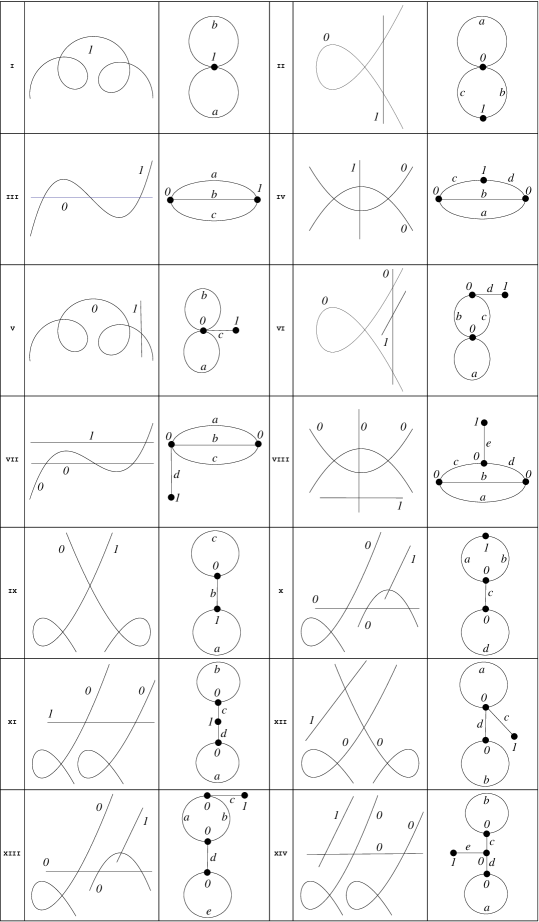
Figure 3. Irreducible components of genus 3 curves and their dual graphs when the dual graphs have genus $2$, i.e. when $\bar{g}=3$ and $g=2$.

	$\ell(\Gamma)$	$\delta_{1}(\Gamma)$	$\tau(\Gamma)$	$\theta(\Gamma)$
$I$	$a+b$	$0$	$\frac{\ell(\Gamma)}{12}$	$0$
$II$	$a+b+c$	$0$	$\frac{\ell(\Gamma)}{12}$	$\frac{8bc}{b+c}$
$III$	$a+b+c$	$0$	$\frac{\ell(\Gamma)}{12}-\frac{abc}{6(ab+ac+bc)}$	$\frac{6abc}{ab+ac+bc}$
$IV$	$a+b+c+d$	$0$	$\frac{\ell(\Gamma)}{12}-\frac{ab(c+d)}{6(ab+(a+b)(c+d))}$	$\frac{6ab(c+d)+8(a+b)cd}{ab+(a+b)(c+d)}$
$V$	$a+b+c$	$c$	$\frac{\ell(\Gamma)}{12}+\frac{c}{6}$	$6c$
$VI$	$a+b+c+d$	$d$	$\frac{\ell(\Gamma)}{12}+\frac{d}{6}$	$6d+\frac{8bc}{b+c}$
$VII$	$a+b+c+d$	$d$	$\frac{\ell(\Gamma)}{12}+\frac{d}{6}-\frac{abc}{6(ab+ac+bc)}$	$6d+\frac{6abc}{ab+ac+bc}$
$VIII$	$a+b+c+d+e$	$e$	$\frac{\ell(\Gamma)}{12}+\frac{e}{6}-\frac{ab(c+d)}{6(ab+(a+b)(c+d))}$	$6e+\frac{6ab(c+d)+8(a+b)cd}{ab+(a+b)(c+d)}$
$IX$	$a+b+c$	$b$	$\frac{\ell(\Gamma)}{12}+\frac{b}{6}$	$6b$
$X$	$a+b+c+d$	$c$	$\frac{\ell(\Gamma)}{12}+\frac{c}{6}$	$6c+\frac{8ab}{a+b}$
$XI$	$a+b+c+d$	$c+d$	$\frac{\ell(\Gamma)}{12}+\frac{c+d}{6}$	$6(c+d)$
$XII$	$a+b+c+d$	$c+d$	$\frac{\ell(\Gamma)}{12}+\frac{c+d}{6}$	$6(c+d)$
$XIII$	$a+b+c+d+e$	$d+c$	$\frac{\ell(\Gamma)}{12}+\frac{c+d}{6}$	$6(c+d)+\frac{8ab}{a+b}$
$XIV$	$a+b+c+d+e$	$c+d+e$	$\frac{\ell(\Gamma)}{12}+\frac{c+d+e}{6}$	$6(c+d+e)$

Table 4. Pm-graph invariants when $g(\Gamma)=2$, part 1. We have $\delta_{0}(\Gamma)=\ell(\Gamma)-\delta_{1}(\Gamma)$, and $\delta_{i}(\Gamma)=0$ for all $i\geq 2$.

	$\varphi(\Gamma)$	$\lambda(\Gamma)$	$\epsilon(\Gamma)$
$I$	$\frac{\ell(\Gamma)}{9}$	$\frac{3\ell(\Gamma)}{28}$	$\frac{2\ell(\Gamma)}{9}$
$II$	$\frac{\ell(\Gamma)}{9}+\frac{2bc}{3(b+c)}$	$\frac{3\ell(\Gamma)}{28}+\frac{bc}{7(b+c)}$	$\frac{2\ell(\Gamma)}{9}+\frac{4bc}{3(b+c)}$
$III$	$\frac{\ell(\Gamma)}{9}-\frac{2abc}{9(ab+ac+bc)}$	$\frac{3\ell(\Gamma)}{28}+\frac{abc}{28(ab+ac+bc)}$	$\frac{2\ell(\Gamma)}{9}+\frac{5abc}{9(ab+ac+bc)}$
$IV$	$\frac{\ell(\Gamma)}{9}+\frac{6cd(a+b)-2ab(c+d)}{9(ab+(a+b)(c+d))}$	$\frac{3\ell(\Gamma)}{28}+\frac{4cd(a+b)+ab(c+d)}{28(ab+(a+b)(c+d))}$	$\frac{2\ell(\Gamma)}{9}+\frac{12cd(a+b)+5ab(c+d)}{9(ab+(a+b)(c+d))}$
$V$	$\frac{\ell(\Gamma)}{9}+\frac{11c}{9}$	$\frac{3\ell(\Gamma)}{28}+\frac{5c}{28}$	$\frac{2\ell(\Gamma)}{9}+\frac{13c}{9}$
$VI$	$\frac{\ell(\Gamma)}{9}+\frac{6bc+11d(b+c)}{9(b+c)}$	$\frac{3\ell(\Gamma)}{28}+\frac{4bc+5d(b+c)}{28(b+c)}$	$\frac{2\ell(\Gamma)}{9}+\frac{12bc+13d(b+c)}{9(b+c)}$
$VII$	$\frac{\ell(\Gamma)}{9}+\frac{11d}{9}-\frac{2abc}{9(ab+ac+bc)}$	$\frac{3\ell(\Gamma)}{28}+\frac{5d}{28}+\frac{abc}{28(ab+ac+bc)}$	$\frac{2\ell(\Gamma)}{9}+\frac{13d}{9}+\frac{5abc}{9(ab+ac+bc)}$
$VIII$	$\frac{\ell(\Gamma)+11e}{9}+\frac{6cd(a+b)-2ab(c+d)}{9(ab+(a+b)(c+d))}$	$\frac{3\ell(\Gamma)+5e}{28}+\frac{4cd(a+b)+ab(c+d)}{28(ab+(a+b)(c+d))}$	$\frac{2\ell(\Gamma)+13e}{9}+\frac{12cd(a+b)+5ab(c+d)}{9(ab+(a+b)(c+d))}$
$IX$	$\frac{\ell(\Gamma)}{9}+\frac{11b}{9}$	$\frac{3\ell(\Gamma)}{28}+\frac{5b}{28}$	$\frac{2\ell(\Gamma)}{9}+\frac{13b}{9}$
$X$	$\frac{\ell(\Gamma)}{9}+\frac{6ab+11c(a+b)}{9(a+b)}$	$\frac{3\ell(\Gamma)}{28}+\frac{4ab+5c(a+b)}{28(a+b)}$	$\frac{2\ell(\Gamma)}{9}+\frac{12ab+13c(a+b)}{9(a+b)}$
$XI$	$\frac{\ell(\Gamma)}{9}+\frac{11(c+d)}{9}$	$\frac{3\ell(\Gamma)}{28}+\frac{5(c+d)}{28}$	$\frac{2\ell(\Gamma)}{9}+\frac{13(c+d)}{9}$
$XII$	$\frac{\ell(\Gamma)}{9}+\frac{11(c+d)}{9}$	$\frac{3\ell(\Gamma)}{28}+\frac{5(c+d)}{28}$	$\frac{2\ell(\Gamma)}{9}+\frac{13(c+d)}{9}$
$XIII$	$\frac{\ell(\Gamma)}{9}+\frac{6ab+11(a+b)(c+d)}{9(a+b)}$	$\frac{3\ell(\Gamma)}{28}+\frac{4ab+5(a+b)(c+d)}{28(a+b)}$	$\frac{2\ell(\Gamma)}{9}+\frac{12ab+13(a+b)(c+d)}{9(a+b)}$
$XIV$	$\frac{\ell(\Gamma)}{9}+\frac{11(c+d+e)}{9}$	$\frac{3\ell(\Gamma)}{28}+\frac{5(c+d+e)}{28}$	$\frac{2\ell(\Gamma)}{9}+\frac{13(c+d+e)}{9}$

Table 5. Pm-graph invariants when $g(\Gamma)=2$, part 2.

6. The case $g(\Gamma)=3$

In this section, we consider pm-graphs $(\Gamma,\textbf{q})$ with $g(\Gamma)=3$ and $g=3$. In this case, Equation (2) implies $\textbf{q}(p)=0$ for each vertex $p\in V(\Gamma)$. That is, $(\Gamma,\textbf{q})$ is a simple pm-graph. Using this observation and Remark 2.2, we note that $\upsilon(p)\geq 2$ for each $p\in V(\Gamma)$. Moreover, using Remark 2.4 we can assume that $\upsilon(p)\geq 3$ for each $p\in V(\Gamma)$ for this section. By basic graph theory, this implies $e\geq\frac{3}{2}v$. On the other hand, we have $e=v+2$ since $g=3$. Therefore, we conclude that $1\leq v\leq 4$ for the simple pm-graphs we can have. Based on these observations, Figure 4 illustrates all the pm-graphs satisfying these conditions.

We compute $\tau(\Gamma)$ by using similar techniques as in the previous section except for the pm-graphs in parts $VIII$, $XIII$ and $XIV$ of Figure 4. The simple pm-graph in part $XIV$ is a tetrahedral graph for which we have computed its tau constant in [4, Example 8.4]. We can compute the tau constant for the simple pm-graphs in parts $VIII$ and $XIII$ by using the techniques developed in [4], such as [4, Corollaries 5.3 and 7.4, Propositions 4.6 and 4.5].

As in the previous sections, we compute $\theta(\Gamma)$ by using its definition and determining the resistance values between any two vertices of the pm-graph. Note that computing the resistance matrix of the corresponding graph will also help, as it is done in [9, Example III].

Once the values of $\tau(\Gamma)$ and $\theta(\Gamma)$ are obtained, we compute $\varphi(\Gamma)$, $\lambda(\Gamma)$ and $\epsilon(\Gamma)$ by using Theorem 2.3. As in the previous sections, the topology of $\Gamma$ is the main factor effecting the invariants $\delta_{0}(\Gamma)$ and $\delta_{1}(\Gamma)$.

The results for pm-graphs of types $I$-$XII$ in Figure 4 are given in Table 6, Table 7 and Table 8. Since the values of the invariants are lengthy for the remaining pm-graphs, types $XIII$ and $XIV$, we state them separately in this section.

It is clear from Table 8 and the results for pm-graphs of types $XIII$ and $XIV$ that $\lambda(\Gamma)\geq\frac{3}{28}\ell(\Gamma)$ and $\epsilon(\Gamma)\geq\frac{2}{9}\ell(\Gamma)$ for all pm-graphs in Figure 4, and this lower bounds are attained for the pm-graph in type $I$.

Clearly, Table 7 shows that $\varphi(\Gamma)\geq\frac{1}{9}\ell(\Gamma)$ for pm-graphs of type $I$, $IV$, $V$, $VI$, $VII$, $XI$.

We use Arithmetic-Harmonic Mean inequality for $a$, $b$ ,$c$, i.e., $\frac{a+b+c}{3}-\frac{3}{1/a+1/b+1/c}\geq 0$, to derive $\varphi(\Gamma)\geq\frac{7}{81}\ell(\Gamma)$ for the pm-graphs of types $III$ and $X$. Using the Arithmetic-Harmonic Mean inequality for $b+c$, $d$, $e$ gives $\varphi(\Gamma)\geq\frac{7}{81}\ell(\Gamma)$ for the pm-graph of type $IX$. Similarly, using the Arithmetic-Harmonic Mean inequality for $a$, $b$, $c+d$ gives $\varphi(\Gamma)\geq\frac{7}{81}\ell(\Gamma)$ for the pm-graph of type $XII$.

We note that $\varphi(\Gamma)=\frac{1}{16}\ell(\Gamma)+\frac{7}{36}(\frac{a+b+c+d}{4}-\frac{4}{1/a+1/b+1/c+1/d})$ for the pm-graph of type $II$. Therefore, we obtain $\varphi(\Gamma)\geq\frac{1}{16}\ell(\Gamma)$ by using the Arithmetic-Harmonic Mean inequality for $a$, $b$, $c$ and $d$. In particular, $\varphi(\Gamma)=\frac{1}{16}\ell(\Gamma)$ when $a=b=c=d$.

Computations to find the lower bounds of $\varphi(\Gamma)$ requires more in-depth analysis for pm-graphs of types $VIII$, $XIII$ and $XIV$. Thus, we consider each of these pm-graphs separately.

Pm-graphs of type $VIII$:

Let $H=b^{2}cd+bc^{2}d+bcd^{2}+b^{2}ce+bc^{2}e+b^{2}de-12bcde+c^{2}de+bd^{2}e+cd^{2}e+bce^{2}+bde^{2}+cde^{2}$, $D=ace+abe+cbe+acd+abd+cbd+ced+bed$, $N=14ace+3c^{2}e+14abe+3b^{2}e+3ce^{2}+3be^{2}+14acd+3c^{2}d+14abd+3b^{2}d+3cd^{2}+3bd^{2}$, $M=(c-b)^{2}e+(c-b)^{2}d+c(e-d)^{2}+b(e-d)^{2}$. Clearly, $D$, $N$ and $M$ are nonnegative. We note that $H\geq 0$ by applying Arithmetic-Harmonic Mean inequality for $b$, $c$, $d$ and $e$.

Now we note that $\varphi(\Gamma)=\frac{1}{16}\ell(\Gamma)+\frac{a(N+11M)+14H}{288D}$, which implies that $\varphi(\Gamma)\geq\frac{1}{16}\ell(\Gamma)$. This is the sharp lower bound because $\varphi(\Gamma)=\frac{1}{16}\ell(\Gamma)$ whenever $a=0$ and $b=c=d=e$.

	$\ell(\Gamma)$	$\delta_{1}(\Gamma)$	$\tau(\Gamma)$
$I$	$a+b+c$	$0$	$\frac{\ell(\Gamma)}{12}$
$II$	$a+b+c+d$	$0$	$\frac{\ell(\Gamma)}{12}-\frac{abcd}{3(bcd+a(cd+b(c+d)))}$
$III$	$a+b+c+d$	$0$	$\frac{\ell(\Gamma)}{12}-\frac{abc}{6(ab+ac+bc)}$
$IV$	$a+b+c+d$	$0$	$\frac{\ell(\Gamma)}{12}$
$V$	$a+b+c+d$	$d$	$\frac{\ell(\Gamma)}{12}+\frac{d}{6}$
$VI$	$a+b+c+d+e$	$d+e$	$\frac{\ell(\Gamma)}{12}+\frac{d+e}{6}$
$VII$	$a+b+c+d+e$	$c$	$\frac{\ell(\Gamma)}{12}+\frac{c}{6}$
$VIII$	$a+b+c+d+e$	$0$	$\frac{\ell(\Gamma)}{12}-\frac{abcd+abce+abde+acde+2bcde}{6(abd+acd+bcd+abe+ace+bce+bde+cde)}$
$IX$	$a+b+c+d+e$	$0$	$\frac{\ell(\Gamma)}{12}+\frac{b}{6}$
$X$	$a+b+c+d+e$	$d$	$\frac{\ell(\Gamma)}{12}+\frac{d}{6}-\frac{abc}{6(ab+ac+bc)}$
$XI$	$a+b+c+d+e+f$	$c+d$	$\frac{\ell(\Gamma)}{12}+\frac{c+d}{6}$
$XII$	$a+b+c+d+e+f$	$e$	$\frac{\ell(\Gamma)}{12}+\frac{e}{6}-\frac{ab(c+d)}{6(ab+(a+b)(c+d))}$

Table 6. Values of $\ell(\Gamma)$, $\delta_{1}(\Gamma)$ and $\tau(\Gamma)$ for pm-graphs with $g(\Gamma)=3$ and $\bar{g}=3$. We have $\delta_{0}(\Gamma)=\ell(\Gamma)-\delta_{1}(\Gamma)$, and $\delta_{i}(\Gamma)=0$ for all $i\geq 2$.

	$\theta(\Gamma)$	$\varphi(\Gamma)$
$I$	$0$	$\frac{\ell(\Gamma)}{9}$
$II$	$\frac{8abcd}{bcd+a(cd+b(c+d))}$	$\frac{\ell(\Gamma)}{9}-\frac{7abcd}{9(bcd+a(cd+b(c+d)))}$
$III$	$\frac{6abc}{ab+ac+bc}$	$\frac{\ell(\Gamma)}{9}-\frac{2abc}{9(bc+a(b+c))}$
$IV$	$\frac{8cd}{c+d}$	$\frac{\ell(\Gamma)}{9}+\frac{2cd}{3(c+d)}$
$V$	$6d$	$\frac{\ell(\Gamma)}{9}+\frac{11d}{9}$
$VI$	$6(d+e)$	$\frac{\ell(\Gamma)}{9}+\frac{11(d+e)}{9}$
$VII$	$6c+\frac{8de}{d+e}$	$\frac{\ell(\Gamma)}{9}+\frac{11c}{9}+\frac{2de}{3(d+e)}$
$VIII$	$\frac{6abcd+6abce+6abde+6acde+8bcde}{abd+acd+bcd+abe+ace+bce+bde+cde}$	$\frac{\ell(\Gamma)}{9}-\frac{7bcde+2a(cde+b(de+c(d+e)))}{9(cde+a(b+c)(d+e)+b(de+c(d+e)))}$
$IX$	$\frac{8bcd+8bce+6bde+6cde}{bd+cd+be+ce+de}$	$\frac{\ell(\Gamma)}{9}+\frac{-2(b+c)de+6bc(d+e)}{9(de+(b+c)(d+e))}$
$X$	$6d+\frac{6abc}{ab+ac+bc}$	$\frac{\ell(\Gamma)}{9}+\frac{11d}{9}-\frac{2abc}{9(bc+a(b+c))}$
$XI$	$6(c+d)+\frac{8ef}{e+f}$	$\frac{\ell(\Gamma)}{9}+\frac{11(c+d)}{9}+\frac{2ef}{3(e+f)}$
$XII$	$6e+\frac{6abc+6abd+8acd+8bcd}{ab+(a+b)(c+d)}$	$\frac{\ell(\Gamma)}{9}+\frac{11e}{9}+\frac{6(a+b)cd-2ab(c+d)}{9(ab+(a+b)(c+d))}$

Table 7. Values of $\theta(\Gamma)$ and $\varphi(\Gamma)$ for pm-graphs with $g(\Gamma)=3$ and $\bar{g}=3$.

	$\lambda(\Gamma)$	$\epsilon(\Gamma)$
$I$	$\frac{3\ell(\Gamma)}{28}$	$\frac{2\ell(\Gamma)}{9}$
$II$	$\frac{3\ell(\Gamma)}{28}$	$\frac{2\ell(\Gamma)}{9}+\frac{4abcd}{9(bcd+a(cd+b(c+d)))}$
$III$	$\frac{3\ell(\Gamma)}{28}+\frac{abc}{28(bc+a(b+c))}$	$\frac{2\ell(\Gamma)}{9}+\frac{5abc}{9(bc+a(b+c))}$
$IV$	$\frac{3\ell(\Gamma)}{28}+\frac{cd}{7(c+d)}$	$\frac{2\ell(\Gamma)}{9}+\frac{4cd}{3(c+d)}$
$V$	$\frac{3\ell(\Gamma)}{28}+\frac{5d}{28}$	$\frac{2\ell(\Gamma)}{9}+\frac{13d}{9}$
$VI$	$\frac{3\ell(\Gamma)}{28}+\frac{5(d+e)}{28}$	$\frac{2\ell(\Gamma)}{9}+\frac{13(d+e)}{9}$
$VII$	$\frac{3\ell(\Gamma)}{28}+\frac{5c}{28}+\frac{de}{7(d+e)}$	$\frac{2\ell(\Gamma)}{9}+\frac{13c}{9}+\frac{4de}{3(d+e)}$
$VIII$	$\frac{3\ell(\Gamma)}{28}+\frac{a((c+b)de+bc(d+e))}{28(cde+a(b+c)(d+e)+b(de+c(d+e)))}$	$\frac{2\ell(\Gamma)}{9}+\frac{4bcde+5a(cde+b(de+c(d+e)))}{9(cde+a(b+c)(d+e)+b(de+c(d+e)))}$
$IX$	$\frac{3\ell(\Gamma)}{28}+\frac{(b+c)de+4bc(d+e)}{28(de+(b+c)(d+e))}$	$\frac{2\ell(\Gamma)}{9}+\frac{5(b+c)de+12bc(d+e)}{9(de+(b+c)(d+e))}$
$X$	$\frac{3\ell(\Gamma)}{28}+\frac{5d}{28}+\frac{abc}{28(bc+a(b+c))}$	$\frac{2\ell(\Gamma)}{9}+\frac{13d}{9}+\frac{5abc}{9(bc+a(b+c))}$
$XI$	$\frac{3\ell(\Gamma)}{28}+\frac{5(c+d)}{28}+\frac{ef}{7(e+f)}$	$\frac{2\ell(\Gamma)}{9}+\frac{13(c+d)}{9}+\frac{4ef}{3(e+f)}$
$XII$	$\frac{3\ell(\Gamma)}{28}+\frac{5e}{28}+\frac{4(a+b)cd+ab(c+d)}{28(ab+(a+b)(c+d))}$	$\frac{2\ell(\Gamma)}{9}+\frac{13e}{9}+\frac{12(a+b)cd+5ab(c+d)}{9(ab+(a+b)(c+d))}$

Table 8. Values of $\lambda(\Gamma)$ and $\epsilon(\Gamma)$ for pm-graphs with $g(\Gamma)=3$ and $\bar{g}=3$.

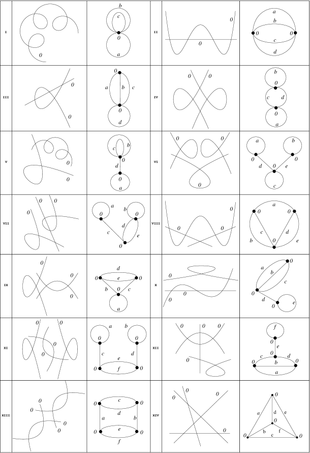
Figure 4. Irreducible components of genus 3 curves and their dual graphs when the dual graphs have genus 3, i.e. when $\bar{g}=g=3$.

Pm-graphs of type $XIII$:

Let $\Gamma$ be a pm-graph as illustrated in $XIII$ in Figure 4. In this case, we have $\ell(\Gamma)=a+b+c+d+e+f$, $\delta_{0}(\Gamma)=\ell(\Gamma)$, and $\delta_{i}(\Gamma)=0$ for all $i\geq 1$. Moreover,

$$\tau(\Gamma) =\frac{\ell(\Gamma)}{12}-\frac{A+2C}{6D}, \theta(\Gamma) =\frac{6A+8B+8C}{D},$$

$$\varphi(\Gamma) =\frac{\ell(\Gamma)}{9}-\frac{2A-6B+7C}{9D}, \lambda(\Gamma) =\frac{3\ell(\Gamma)}{28}+\frac{A+4B}{28D},$$

and

$$\epsilon(\Gamma)=\frac{2}{9}\ell(\Gamma)+\frac{5A+12B+4C}{9D},$$

where $A=acde+bcde+acdf+bcdf+acef+bcef+adef+bdef$, $B=abce+abde+abcf+abdf$, $C=cdef$ and $D=(a+b)ce+(a+b)de+cde+(a+b)cf+(a+b)df+cdf+cef+def)$.

Let $H=c^{2}de+cd^{2}e+cde^{2}+c^{2}df+cd^{2}f+c^{2}ef-12cdef+d^{2}ef+ce^{2}f+de^{2}f+cdf^{2}+cef^{2}+def^{2}$, $N=14(a+b)ce+3c^{2}e+14(a+b)de+3d^{2}e+3ce^{2}+3de^{2}+14(a+b)cf+3c^{2}f+14(a+b)df+3d^{2}f+3cf^{2}+3df^{2}$, $M=(c-d)^{2}e+(c-d)^{2}f+c(e-f)^{2}+d(e-f)^{2}$. We see that $D$, $N$ and $M$ are nonnegative, and note that $H\geq 0$ by applying Arithmetic-Harmonic Mean inequality for $c$, $d$, $e$ and $f$.

Now we note that $\varphi(\Gamma)=\frac{1}{16}\ell(\Gamma)+\frac{(a+b)(N+11M)+14H+192ab(c+d)(e+f)}{288D}$, which implies that $\varphi(\Gamma)\geq\frac{1}{16}\ell(\Gamma)$. This is the sharp lower bound because $\varphi(\Gamma)=\frac{1}{16}\ell(\Gamma)$ whenever $a=b=0$ and $c=d=e=f$.

Pm-graphs of type $XIV$:

Let $\Gamma$ be a pm-graph as illustrated in $XIV$ in Figure 4. In this case, we have $\ell(\Gamma)=a+b+c+d+e+f$, $\delta_{0}(\Gamma)=\ell(\Gamma)$, and $\delta_{i}(\Gamma)=0$ for all $i\geq 1$. Moreover,

$$\tau(\Gamma) =\frac{\ell(\Gamma)}{12}-\frac{A+2B}{6C}, \theta(\Gamma) =\frac{6A+8B}{C},$$

$$\varphi(\Gamma) =\frac{\ell(\Gamma)}{9}-\frac{2A+7B}{9C}, \lambda(\Gamma) =\frac{3\ell(\Gamma)}{28}+\frac{A}{28C},$$

$$\epsilon(\Gamma) =\frac{2}{9}\ell(\Gamma)+\frac{5A+4B}{9C},$$

where $A=abcd+abce+abde+acde+abcf+abdf+bcdf+acef+bcef+adef+bdef+cdef$, $B=bcde+acdf+abef$, and $C=abd+acd+bcd+abe+ace+bce+bde+cde+abf+acf+bcf+adf+cdf+aef+bef+def$.

We first show that $\tau(\Gamma)\geq\frac{5}{96}\ell(\Gamma)$, where the equality holds whenever $a=b=c=d=e=f$. We have $\tau(\Gamma)=\frac{5}{96}\ell(\Gamma)+\frac{3M-7A-20B}{96C}$ where $M=a^{2}bd+a^{2}be+a^{2}bf+a^{2}cd+a^{2}ce+a^{2}cf+a^{2}df+a^{2}ef+ab^{2}d+ab^{2}e+ab^{2}f+abd^{2}+abe^{2}+abf^{2}+ac^{2}d+ac^{2}e+ac^{2}f+acd^{2}+ace^{2}+acf^{2}+ad^{2}f+adf^{2}+ae^{2}f+aef^{2}+b^{2}cd+b^{2}ce+b^{2}cf+b^{2}de+b^{2}ef+bc^{2}d+bc^{2}e+bc^{2}f+bcd^{2}+bce^{2}+bcf^{2}+bd^{2}e+bde^{2}+be^{2}f+bef^{2}+c^{2}de+c^{2}df+cd^{2}e+cd^{2}f+cde^{2}+cdf^{2}+d^{2}ef+de^{2}f+def^{2}$.

Thus, we see that proving $S:=3M-7A-20B\geq 0$ gives $\tau(\Gamma)\geq\frac{5}{96}\ell(\Gamma)$. Now, we have the following tricky equality

$$\begin{split}S&=2\big{[}be\left((a-f)^{2}+(d-c)^{2}\right)+cd\left((a-f)^{2}+(b-e)^{2}\right)+af\left((e-b)^{2}+(d-c)^{2}\right)\big{]}\\ &\quad+\frac{3}{2}\big{[}bd\left((a-c)^{2}+(a-e)^{2}+(c-e)^{2}\right)+ce\left((b-a)^{2}+(d-a)^{2}+(b-d)^{2}\right)\\ &\quad+ad\left((b-c)^{2}+(b-f)^{2}+(c-f)^{2}\right)+cf\left((a-b)^{2}+(a-d)^{2}+(d-b)^{2}\right)\\ &\quad+bf\left((c-a)^{2}+(e-a)^{2}+(c-e)^{2}\right)+ae\left((b-c)^{2}+(f-b)^{2}+(f-c)^{2}\right)\\ &\quad+ef\left((a-b)^{2}+(a-d)^{2}+(d-b)^{2}\right)+ab\left((d-e)^{2}+(d-f)^{2}+(f-e)^{2}\right)\\ &\quad+ac\left((d-e)^{2}+(d-f)^{2}+(e-f)^{2}\right)+df\left((a-c)^{2}+(e-a)^{2}+(e-c)^{2}\right)\\ &\quad+de\left((b-c)^{2}+(b-f)^{2}+(c-f)^{2}\right)+bc\left((d-e)^{2}+(d-f)^{2}+(e-f)^{2}\right)\big{]}\\ &\quad+\frac{1}{2}\big{[}cd(a-b)^{2}+be(a-c)^{2}+af(b-c)^{2}+be(a-d)^{2}+af(b-d)^{2}+cd(a-e)^{2}\\ &\quad+af(c-e)^{2}+af(d-e)^{2}+be\left((c-f)^{2}+(d-f)^{2}\right)+cd(b-f)^{2}+cd(e-f)^{2}\big{]}.\end{split}$$

Thus, $S$ is a sum of positive terms. This gives

(5) $$\begin{split}3M-7A-20B\geq 0,\quad\text{ and so }\quad\tau(\Gamma)\geq\frac{5}{96}\ell(\Gamma).\end{split}$$

Now, we consider $\varphi(\Gamma)$. We note that $\varphi(\Gamma)=\frac{17}{288}\ell(\Gamma)$ whenever $\Gamma$ has equal edge lengths, i.e., if $a=b=c=d=e=f$. Next, we show that this is the sharp lower bound for $\Gamma$ and so for all pm-graphs of $\bar{g}=3$.

Claim: $\varphi(\Gamma)\geq\frac{17}{288}\ell(\Gamma)$.

Proof of Claim: It is worth mentioning that we are unable to give a proof of this inequality neither by utilizing arithmetic harmonic mean inequalities partially or fully as in the previous cases nor by using any other well-known inequality in literature. Instead we found the following highly tricky and technical proof after spending extensive time on this problem.

Since $\varphi(\Gamma)=\frac{17}{288}\ell(\Gamma)+\frac{15D-19A-164B}{C}$, where $A$, $B$ and $C$ are as above and $D$ is as follows:

$D=a^{2}bd+a^{2}be+a^{2}bf+a^{2}cd+a^{2}ce+a^{2}cf+a^{2}df+a^{2}ef+ab^{2}d+ab^{2}e+ab^{2}f+abd^{2}+abe^{2}+abf^{2}+ac^{2}d+ac^{2}e+ac^{2}f+acd^{2}+ace^{2}+acf^{2}+ad^{2}f+adf^{2}+ae^{2}f+aef^{2}+b^{2}cd+b^{2}ce+b^{2}cf+b^{2}de+b^{2}ef+bc^{2}d+bc^{2}e+bc^{2}f+bcd^{2}+bce^{2}+bcf^{2}+bd^{2}e+bde^{2}+be^{2}f+bef^{2}+c^{2}de+c^{2}df+cd^{2}e+cd^{2}f+cde^{2}+cdf^{2}+d^{2}ef+de^{2}f+def^{2}$

Therefore, it is enough to show that the following inequality holds to prove the claim:

(6) $$\begin{split}15D-19A-164B\geq 0\end{split}$$

The proof of this inequality consists of eight similar cases that depends on the comparison of the involved variables. The idea is to express $15D-19A-164B$ as sums squares and nonnegative terms. Lets denote this term by $R$, i.e., we set $R:=15D-19A-164B$.

Case I: Suppose $a\geq f$, $b\geq e$ and $c\geq d$:

We have

$$\begin{split}R&=2\big{[}cd(b+e-a-f)^{2}+be(c+d-a-f)^{2}+af(c+d-b-e)^{2}\big{]}\\ &\quad+13\big{[}be(a-c+d-f)^{2}+cd(a-b+e-f)^{2}+af(-b+c-d+e)^{2}\big{]}\\ &\quad+15\big{[}de(b-c)^{2}+bd(c-e)^{2}+df(c-a)^{2}+da(c-f)^{2}+ab(e-f)^{2}+ac(d-f)^{2}\\ &\quad+ae(b-f)^{2}+bc(d-e)^{2}+bf(a-e)^{2}+ce(b-d)^{2}+cf(a-d)^{2}+ef(a-b)^{2}\big{]}\\ &\quad+11\big{[}cd(a-f)(b-e)+be(a-f)(c-d)+af(b-e)(c-d)\big{]}\\ &\quad+15T_{1},\end{split}$$

where $T_{1}=a^{2}bd+a^{2}ce+ab^{2}d+abd^{2}-2abde-2abdf+ac^{2}e-2acde+ace^{2}-2acef+b^{2}cf+bc^{2}f-2bcdf-2bcef+bcf^{2}+d^{2}ef+de^{2}f+def^{2}$.

By the assumptions in this case, we have $a-f\geq 0$, $b-e\geq 0$ and $c-d\geq 0$. Therefore, to prove $R\geq 0$, it will be enough to show $T_{1}\geq 0$. Again by the assumptions, we can write $a=f+k$, $b=e+m$ and $c=d+n$ for some nonnegative real numbers $k$, $m$ and $n$. Now substituting these into $T_{1}$ gives

$T_{1}=d^{2}km+2dek^{2}+2dfm^{2}+dk^{2}m+dkm^{2}+e^{2}kn+2efn^{2}+ek^{2}n+ekn^{2}+f^{2}mn+fm^{2}n+fmn^{2}$, which clearly shows that $T_{1}\geq 0$. Hence, $R\geq 0$ in this case.

Case II: Suppose $a\geq f$, $b\geq e$ and $d\geq c$:

We have

$$\begin{split}R&=2\big{[}af(-b+c+d-e)^{2}+be(-a+c+d-f)^{2}+cd(-a+b+e-f)^{2}\big{]}\\ &\quad+13\big{[}be(a+c-d-f)^{2}+cd(a-b+e-f)^{2}+af(-b-c+d+e)^{2}\big{]}\\ &\quad+15\big{[}ae(b-f)^{2}+ab(e-f)^{2}+bf(a-e)^{2}+ef(a-b)^{2}+df(c-a)^{2}+ad(c-f)^{2}\\ &\quad+ac(d-f)^{2}+cf(a-d)^{2}+bd(c-e)^{2}+bc(d-e)^{2}+ce(b-d)^{2}+de(b-c)^{2}\big{]}\\ &\quad+11\big{[}cd(a-f)(b-e)+be(a-f)(d-c)+af(b-e)(d-c)\big{]}\\ &\quad+15T_{2},\end{split}$$

where $T_{2}=a^{2}bd+a^{2}ce+ab^{2}d-2abce-2abcf+abd^{2}+ac^{2}e-2acde+ace^{2}-2adef+b^{2}cf+bc^{2}f-2bcdf+bcf^{2}-2bdef+d^{2}ef+de^{2}f+def^{2}$.

By the assumptions in this case, we have $a-f\geq 0$, $b-e\geq 0$ and $d-c\geq 0$. Therefore, to prove $R\geq 0$, it will be enough to show $T_{2}\geq 0$. Again by the assumptions, we can write $a=f+k$, $b=e+m$ and $d=c+n$ for some nonnegative real numbers $k$, $m$ and $n$. Now substituting these into $T_{2}$ gives $T_{2}=c^{2}km+2cek^{2}+2cfm^{2}+ck^{2}m+ckm^{2}+2ckmn+e^{2}kn+2efn^{2}+ek^{2}n+2ekmn+ekn^{2}+f^{2}mn+2fkmn+fm^{2}n+fmn^{2}+k^{2}mn+km^{2}n+kmn^{2}$. This shows that $T_{2}\geq 0$. Hence, $R\geq 0$ in this case.

Case III: Suppose $a\geq f$, $e\geq b$ and $c\geq d$:

We have

$$\begin{split}R&=2\big{[}af(-b+c+d-e)^{2}+be(-a+c+d-f)^{2}+cd(-a+b+e-f)^{2}\big{]}\\ &\quad+13\big{[}cd(a-f+b-e)^{2}+be(a-f-c+d)^{2}+af(c-d+b-e)^{2}\big{]}\\ &\quad+15\big{[}ae(b-f)^{2}+ab(e-f)^{2}+bf(a-e)^{2}+ef(a-b)^{2}+df(c-a)^{2}+ad(c-f)^{2}\\ &\quad+ac(d-f)^{2}+cf(a-d)^{2}+bd(c-e)^{2}+bc(d-e)^{2}+ce(b-d)^{2}+de(b-c)^{2}\big{]}\\ &\quad+11\big{[}cd(a-f)(e-b)+be(a-f)(c-d)+af(e-b)(c-d)\big{]}\\ &\quad+15T_{3},\end{split}$$

where $T_{3}=a^{2}bd+a^{2}ce+ab^{2}d-2abcd-2abcf+abd^{2}-2abde+ac^{2}e+ace^{2}-2adef+b^{2}cf+bc^{2}f-2bcef+bcf^{2}-2cdef+d^{2}ef+de^{2}f+def^{2}$.

By the assumptions in this case, we have $a-f\geq 0$, $e-b\geq 0$ and $c-d\geq 0$. Therefore, to prove $R\geq 0$, it will be enough to show $T_{3}\geq 0$. Again by the assumptions, we can write $a=f+k$, $e=b+m$ and $c=d+n$ for some nonnegative real numbers $k$, $m$ and $n$. Now substituting these into $T_{3}$ gives $T_{3}=b^{2}kn+2bdk^{2}+2bfn^{2}+bk^{2}n+2bkmn+bkn^{2}+d^{2}km+2dfm^{2}+dk^{2}m+dkm^{2}+2dkmn+f^{2}mn+2fkmn+fm^{2}n+fmn^{2}+k^{2}mn+km^{2}n+kmn^{2}$, which shows that $T_{3}\geq 0$. Hence, $R\geq 0$ in this case.

Case IV: Suppose $a\geq f$, $e\geq b$ and $d\geq c$:

We have

$$\begin{split}R&=2\big{[}af(-b+c+d-e)^{2}+be(-a+c+d-f)^{2}+cd(-a+b+e-f)^{2}\big{]}\\ &\quad+13\big{[}be(a+c-d-f)^{2}+cd(a+b-e-f)^{2}+af(b-c+d-e)^{2}\big{]}\\ &\quad+15\big{[}ae(b-f)^{2}+ab(e-f)^{2}+bf(a-e)^{2}+ef(a-b)^{2}+df(c-a)^{2}+ad(c-f)^{2}\\ &\quad+ac(d-f)^{2}+cf(a-d)^{2}+bd(c-e)^{2}+bc(d-e)^{2}+ce(b-d)^{2}+de(b-c)^{2}\big{]}\\ &\quad+11\big{[}cd(a-f)(e-b)+be(a-f)(d-c)+af(e-b)(d-c)\big{]}\\ &\quad+15T_{4},\end{split}$$

where $T_{4}=a^{2}bd+a^{2}ce+ab^{2}d-2abcd-2abce+abd^{2}-2abdf+ac^{2}e+ace^{2}-2acef+b^{2}cf+bc^{2}f+bcf^{2}-2bdef-2cdef+d^{2}ef+de^{2}f+def^{2}$.

By the assumptions in this case, we have $a-f\geq 0$, $e-b\geq 0$ and $d-c\geq 0$. Therefore, to prove $R\geq 0$, it will be enough to show $T_{4}\geq 0$. Again by the assumptions, we can write $a=f+k$, $e=b+m$ and $d=c+n$ for some nonnegative real numbers $k$, $m$ and $n$. Now substituting these into $T_{4}$ gives $T_{4}=b^{2}kn+2bck^{2}+2bfn^{2}+bk^{2}n+bkn^{2}+c^{2}km+2cfm^{2}+ck^{2}m+ckm^{2}+f^{2}mn+fm^{2}n+fmn^{2}$, which clearly shows that $T_{4}\geq 0$. Hence, $R\geq 0$ in this case.

Case V: Suppose $f\geq a$, $b\geq e$ and $c\geq d$:

We have

$$\begin{split}R&=2\big{[}af(-b+c+d-e)^{2}+be(-a+c+d-f)^{2}+cd(-a+b+e-f)^{2}\big{]}\\ &\quad+13\big{[}be(-a-c+d+f)^{2}+cd(-a-b+e+f)^{2}+af(-b+c-d+e)^{2}\big{]}\\ &\quad+15\big{[}ae(b-f)^{2}+ab(e-f)^{2}+bf(a-e)^{2}+ef(a-b)^{2}+df(c-a)^{2}+ad(c-f)^{2}\\ &\quad+ac(d-f)^{2}+cf(a-d)^{2}+bd(c-e)^{2}+bc(d-e)^{2}+ce(b-d)^{2}+de(b-c)^{2}\big{]}\\ &\quad+11\big{[}af(b-e)(c-d)+cd(f-a)(b-e)+be(f-a)(c-d)\big{]}\\ &\quad+15T_{5},\end{split}$$

where $T_{5}=a^{2}bd+a^{2}ce+ab^{2}d-2abcd-2abce+abd^{2}-2abdf+ac^{2}e+ace^{2}-2acef+b^{2}cf+bc^{2}f+bcf^{2}-2bdef-2cdef+d^{2}ef+de^{2}f+def^{2}$.

By the assumptions in this case, we have $f-a\geq 0$, $b-e\geq 0$ and $c-d\geq 0$. Therefore, to prove $R\geq 0$, it will be enough to show $T_{5}\geq 0$. Again by the assumptions, we can write $f=a+k$, $b=e+m$ and $c=d+n$ for some nonnegative real numbers $k$, $m$ and $n$. Now substituting these into $T_{5}$ gives $T_{5}=a^{2}mn+2adm^{2}+2aen^{2}+2akmn+am^{2}n+amn^{2}+d^{2}km+2dek^{2}+dk^{2}m+dkm^{2}+2dkmn+e^{2}kn+ek^{2}n+2ekmn+ekn^{2}+k^{2}mn+km^{2}n+kmn^{2}$. Thus, $T_{5}\geq 0$. Hence, $R\geq 0$ in this case.

Case VI: Suppose $f\geq a$, $b\geq e$ and $d\geq c$:

We have

$$\begin{split}R&=2\big{[}af(-b+c+d-e)^{2}+be(-a+c+d-f)^{2}+cd(-a+b+e-f)^{2}\big{]}\\ &\quad+13\big{[}be(-a+c-d+f)^{2}+cd(-a-b+e+f)^{2}+af(-b-c+d+e)^{2}\big{]}\\ &\quad+15\big{[}ae(b-f)^{2}+ab(e-f)^{2}+bf(a-e)^{2}+ef(a-b)^{2}+df(c-a)^{2}+ad(c-f)^{2}\\ &\quad+ac(d-f)^{2}+cf(a-d)^{2}+bd(c-e)^{2}+bc(d-e)^{2}+ce(b-d)^{2}+de(b-c)^{2}\big{]}\\ &\quad+11\big{[}af(b-e)(d-c)+cd(f-a)(b-e)+be(f-a)(d-c)\big{]}\\ &\quad+15T_{6},\end{split}$$

where $T_{6}=a^{2}bd+a^{2}ce+ab^{2}d-2abcd-2abcf+abd^{2}-2abde+ac^{2}e+ace^{2}-2adef+b^{2}cf+bc^{2}f-2bcef+bcf^{2}-2cdef+d^{2}ef+de^{2}f+def^{2}$.

By the assumptions in this case, we have $f-a\geq 0$, $b-e\geq 0$ and $d-c\geq 0$. Therefore, to prove $R\geq 0$, it will be enough to show $T_{6}\geq 0$. Again by the assumptions, we can write $f=a+k$, $b=e+m$ and $d=c+n$ for some nonnegative real numbers $k$, $m$ and $n$. Now substituting these into $T_{6}$ gives $T_{6}=a^{2}mn+2acm^{2}+2aen^{2}+am^{2}n+amn^{2}+c^{2}km+2cek^{2}+ck^{2}m+ckm^{2}+e^{2}kn+ek^{2}n+ekn^{2}$, so $T_{6}\geq 0$. Hence, $R\geq 0$ in this case.

Case VII: Suppose $f\geq a$, $e\geq b$ and $c\geq d$:

We have

$$\begin{split}R&=2\big{[}af(-b+c+d-e)^{2}+be(-a+c+d-f)^{2}+cd(-a+b+e-f)^{2}\big{]}\\ &\quad+13\big{[}be(-a-c+d+f)^{2}+cd(-a+b-e+f)^{2}+af(b+c-d-e)^{2}\big{]}\\ &\quad+15\big{[}ae(b-f)^{2}+ab(e-f)^{2}+bf(a-e)^{2}+ef(a-b)^{2}+df(c-a)^{2}+ad(c-f)^{2}\\ &\quad+ac(d-f)^{2}+cf(a-d)^{2}+bd(c-e)^{2}+bc(d-e)^{2}+ce(b-d)^{2}+de(b-c)^{2}\big{]}\\ &\quad+11\big{[}af(e-b)(c-d)+be(f-a)(c-d)+cd(f-a)(e-b)\big{]}\\ &\quad+15T_{7},\end{split}$$

where $T_{7}=a^{2}bd+a^{2}ce+ab^{2}d-2abce-2abcf+abd^{2}+ac^{2}e-2acde+ace^{2}-2adef+b^{2}cf+bc^{2}f-2bcdf+bcf^{2}-2bdef+d^{2}ef+de^{2}f+def^{2}$

By the assumptions in this case, we have $f-a\geq 0$, $e-b\geq 0$ and $c-d\geq 0$. Therefore, to prove $R\geq 0$, it will be enough to show $T_{7}\geq 0$. Again by the assumptions, we can write $f=a+k$, $e=b+m$ and $c=d+n$ for some nonnegative real numbers $k$, $m$ and $n$. Now substituting these into $T_{7}$ gives $T_{7}=a^{2}mn+2abn^{2}+2adm^{2}+am^{2}n+amn^{2}+b^{2}kn+2bdk^{2}+bk^{2}n+bkn^{2}+d^{2}km+dk^{2}m+dkm^{2}$, which clearly shows that $T_{7}\geq 0$. Hence, $R\geq 0$ in this case.

Case VIII: Suppose $f\geq a$, $e\geq b$ and $d\geq c$:

We have

$$\begin{split}R&=2\big{[}af(-b+c+d-e)^{2}+be(-a+c+d-f)^{2}+cd(-a+b+e-f)^{2}\big{]}\\ &\quad+13\big{[}be(-a+c-d+f)^{2}+cd(-a+b-e+f)^{2}+af(b-c+d-e)^{2}\big{]}\\ &\quad+15\big{[}ae(b-f)^{2}+ab(e-f)^{2}+bf(a-e)^{2}+ef(a-b)^{2}+df(c-a)^{2}+ad(c-f)^{2}\\ &\quad+ac(d-f)^{2}+cf(a-d)^{2}+bd(c-e)^{2}+bc(d-e)^{2}+ce(b-d)^{2}+de(b-c)^{2}\big{]}\\ &\quad+11\big{[}af(e-b)(d-c)+be(f-a)(d-c)+cd(f-a)(e-b)\big{]}\\ &\quad+15T_{8},\end{split}$$

where $T_{8}=a^{2}bd+a^{2}ce+ab^{2}d+abd^{2}-2abde-2abdf+ac^{2}e-2acde+ace^{2}-2acef+b^{2}cf+bc^{2}f-2bcdf-2bcef+bcf^{2}+d^{2}ef+de^{2}f+def^{2}$.

By the assumptions in this case, we have $f-a\geq 0$, $e-b\geq 0$ and $d-c\geq 0$. Therefore, to prove $R\geq 0$, it will be enough to show $T_{8}\geq 0$. Again by the assumptions, we can write $f=a+k$, $e=b+m$ and $d=c+n$ for some nonnegative real numbers $k$, $m$ and $n$. Now substituting these into $T_{8}$ gives $T_{8}=a^{2}mn+2abn^{2}+2acm^{2}+2akmn+am^{2}n+amn^{2}+b^{2}kn+2bck^{2}+bk^{2}n+2bkmn+bkn^{2}+c^{2}km+ck^{2}m+ckm^{2}+2ckmn+k^{2}mn+km^{2}n+kmn^{2}$. This clearly shows that $T_{8}\geq 0$. Hence, $R\geq 0$ in this case.

Next, we give a summary of the inequalities that we established so far. If $(\Gamma,\textbf{q})$ is a pm-graph of $\bar{g}=3$ that is not a single point, then we showed that we have the following equalities and sharp lower bounds:

We have $\lambda(\Gamma)=\frac{2}{7}\ell(\Gamma)$ and $\epsilon(\Gamma)=\frac{5}{3}\ell(\Gamma)$ if $g=0$, and $\lambda(\Gamma)\geq\frac{3}{28}\ell(\Gamma)$ and $\epsilon(\Gamma)\geq\frac{2}{9}\ell(\Gamma)$ if $1\leq g\leq 3$.

If $g=0$, $\varphi(\Gamma)=\frac{4}{3}\ell(\Gamma)$, and if $g=1$, $\varphi(\Gamma)\geq\frac{1}{9}\ell(\Gamma)$. When $g=2$, $\varphi(\Gamma)\geq\frac{7}{81}\ell(\Gamma)$. Finally, $\varphi(\Gamma)\geq\frac{17}{288}\ell(\Gamma)$ if $g=3$.

For any nonnegative six real numbers $a$, $b$, $c$, $d$, $e$ and $f$, we showed (for pm-graph of type XIV in Figure 4) that

(7) $$\begin{split}\frac{15}{32}(a+b+c+d+e+f)-\frac{7(abef+acdf+bcde)+2A}{C}\geq 0,\end{split}$$

where $A=cd(b+e)(a+f)+be(c+d)(a+f)+af(c+d)(b+e)$ and $C=cd(a+b+e+f)+af(b+c+d+e)+be(a+c+d+f)+abd+ace+bcf+def$.

The equality in (7) holds if $a=b=c=d=e=f>0$. Similarly, we can rewrite (5) as follows

(8) $$\begin{split}\frac{1}{32}(a+b+c+d+e+f)-\frac{2(abef+acdf+bcde)+A}{C}\geq 0,\end{split}$$

Moreover, if $a+b+c+d+e+f=1$, we can rewrite inequalities (7) and (8) as follows:

(9) $$\begin{split}&15C-224A-64(abef+acdf+bcde)\geq 0,\\ &3C-16A-32(abef+acdf+bcde)\geq 0,\end{split}$$

where the equalities holds iff $a=b=c=d=e=f=\frac{1}{6}.$

Acknowledgements: This work is supported by The Scientific and Technological Research Council of Turkey-TUBITAK (Project No: 110T686).

References

[1] M. Baker and X. Faber, Metrized graphs, Laplacian operators, and
electrical networks, Contemporary Mathematics 415, Proceedings of the Joint Summer Research Conference
on Quantum Graphs and Their Applications; Berkolaiko, G; Carlson, R; Fulling, S. A.; Kuchment,
P. Snowbird, Utah, 2006, pp. 15-33.
[2] M. Baker and R. Rumely, Harmonic analysis on metrized graphs,
Canadian J. Math: 59, No. 2, (2007), 225–275.
[3] Z. Cinkir, The Tau Constant of Metrized Graphs,
Thesis at University of Georgia, Athens, GA., 2007.
[4] Z. Cinkir, The tau constant of a metrized graph and its behavior under graph operations, The Electronic Journal of Combinatorics, Volume 18, (1), (2011), P81.
[5] Z. Cinkir, The tau constant and the edge connectivity of a metrized graph,
The Electronic Journal of Combinatorics, Volume 19, (4), (2012), P46.
[6] Z. Cinkir, Zhang’s conjecture and the effective Bogomolov conjecture over function fields, Invent. Math., Volume 183, Number 3, (2011), 517–562.
[7] Z. Cinkir, The tau constant and the discrete Laplacian matrix of a metrized graph, European Journal of Combinatorics, Volume 32, Issue 4, (2011), 639–655.
[8] Z. Cinkir, Computation of Polarized Metrized Graph Invariants By Using Discrete Laplacian Matrix, submitted.
The first version is available at http://arxiv.org/abs/1202.4641.
[9] Z. Cinkir, Explicit Computation of Certain Arakelov-Green Functions, To Appear in Kyoto Journal of
Mathematics.
The first version is available at http://arxiv.org/abs/1304.0478v1.
[10] X. W. C. Faber, The geometric bogomolov conjecture for curves of small genus,
Experiment. Math., 18(3), (2009), 347–367.
[11] R. D. Jong, Admissible constants of genus curves, Bull. London Math. Soc., 42, (2010), 405–411.
[12] R. D. Jong, Second variation of Zhang’s lambda-invariant on the moduli space of curves. To appear in
American Journal of Mathematics.
[13] U. Kühn and J. S. Müller, Lower Bounds on the Arithmetic Self-Intersection Number of the Relative Dualizing Sheaf on Arithmetic Surfaces.
Available at http://arxiv.org/abs/0906.2056.
[14] A. Moriwaki, Bogomolov conjecture over function fields for stable curves with only
irreducible fibers, Comp. Math. 105, CMP 97:10, (1997), 125–140.
[15] A. Moriwaki, Bogomolov conjecture for curves of genus over function fields,
J. Math. Kyoto Univ., 36, CMP 97:11, (1996), 687–695.
[16] L. Szpiro, Séminaire sur les pinceaux de courbes de genre au moins deux, Astérisque, Volume 86, (3), (1981), 44–78.
[17] L. Szpiro, Sur les propri t s num riques du dualisant relatif d une surface arithm thique. The Grothendieck Festschrift, Progress in Mathematics, Volume 88, (1990), 229–246.
[18] K. Yamaki, Graph invariants and the positivity of the height of the Gross-Schoen cycle for some curves,
Manuscripta Mathematica, 131, (2010), 149–177.
[19] K. Yamaki, Effective calculation of the geometric height and the Bogomolov
conjecture for hyperelliptic curves over function fields,
J. Math. Kyoto Univ., 48-2, (2008), 401–443.
[20] K. Yamaki, Geometric Bogomolov’s conjecture for curves of genus over function fields,
J. Math. Kyoto Univ., 42-1, (2002), 57–81.
[21] S. Zhang, Admissible pairing on a curve,
Invent. Math., 112, (1993), 171–193.
[22] S. Zhang, Gross–Schoen cycles and dualising sheaves,
Invent. Math., 179, (2010), 1–73