Overview of Constrained PARAFAC Models

Abstract

In this paper, we present an overview of constrained PARAFAC models where the constraints model linear dependencies among columns of the factor matrices of the tensor decomposition, or alternatively, the pattern of interactions between different modes of the tensor which are captured by the equivalent core tensor. Some tensor prerequisites with a particular emphasis on mode combination using Kronecker products of canonical vectors that makes easier matricization operations, are first introduced. This Kronecker product based approach is also formulated in terms of the index notation, which provides an original and concise formalism for both matricizing tensors and writing tensor models. Then, after a brief reminder of PARAFAC and Tucker models, two families of constrained tensor models, the co-called PARALIND/CONFAC and PARATUCK models, are described in a unified framework, for $N^{th}$ order tensors. New tensor models, called nested Tucker models and block PARALIND/CONFAC models, are also introduced. A link between PARATUCK models and constrained PARAFAC models is then established. Finally, new uniqueness properties of PARATUCK models are deduced from sufficient conditions for essential uniqueness of their associated constrained PARAFAC models.

I Introduction

Tensor calculus was introduced in differential geometry, at the end of the $19^{th}$ century, and then tensor analysis was developed in the context of Einstein’s theory of general relativity, with the introduction of index notation, the so-called Einstein summation convention, at the beginning of the $20^{th}$ century, which allows to simplify and shorten physics equations involving tensors. Index notation is also useful for simplifying multivariate statistical calculations, particularly those involving cumulant tensors [1]. Generally speaking, tensors are used in physics and differential geometry for characterizing the properties of a physical system, representing fundamental laws of physics, and defining geometrical objects whose components are functions. When these functions are defined over a continuum of points of a mathematical space, the tensor forms what is called a tensor field, a generalization of vector field used to solve problems involving curved surfaces or spaces, as it is the case of curved space-time in general relativity. From a mathematical point of view, two other approaches are possible for defining tensors, in terms of tensor products of vector spaces, or multilinear maps. Symmetric tensors can also be linked with homogeneous polynomials [2].

After first tensor developments by mathematicians and physicists, the need of analysing collections of data matrices that can be seen as three-way data arrays, gave rise to three-way models for data analysis, with the pioneering works of Tucker (1966) in psychometrics [3], and Harshman (1970) in phonetics [4], who proposed what is now referred to as the Tucker and the PARAFAC (parallel factor) decompositions/models, respectively. PARAFAC decompositions were independently proposed by Carroll and Chang in 1970 [5] under the name CANDECOMP (canonical decomposition), then called CP (for CANDECOMP/PARAFAC) in [6]. For an history of the development of multi-way models in the context of data analysis, see [7]. Since the nineties, multi-way analysis has known a growing success in chemistry and especially in chemometrics. See Bro’s thesis (1998) [8] and the book by Smilde et al. (2004) [9] for a description of various chemical applications of three-way models, with a pedagogical presentation of these models and of various algorithms for estimating their parameters. At the same period, tensor tools were developed for signal processing applications, more particularly for solving the so-called blind source separation (BSS) problem using cumulant tensors. See [10], [11], [12], and De Lathauwer’s thesis [13] where the concept of HOSVD (high order singular value decomposition) is introduced, a tensor tool generalizing the standard matrix SVD to arrays of order higher than two. A recent overview of BSS approaches and applications can be found in the handbook co-edited by Comon and Jutten [14].

Nowadays, (high order) tensors, also called multi-way arrays in the data analysis community, play an important role in many fields of application for representing and analysing multidimensional data, as in psychometrics, chemometrics, food industry, environmental sciences, signal/image processing, computer vision, neuroscience, information sciences, data mining, pattern recognition, among many others. Then, they are simply considered as multidimensional arrays of numbers, constituting a generalization of vectors and matrices that are first- and second-order tensors respectively, to orders higher than two. Tensor models, also called tensor decompositions, are very useful for analysing multidimensional data under the form of signals, images, speech, music sequences, or texts, and also for designing new systems as it is the case of wireless communication systems since the publication of the seminal paper by Sidiropoulos et al., in 2000 [15]. Besides the references already cited, overviews of tensor tools, models, algorithms, and applications can be found in [16], [17], [18], [19].

Tensor models incorporating constraints (sparsity; non-negativity; smoothness; symmetry; column orthonormality of factor matrices; Hankel, Toeplitz, and Vandermonde structured matrix factors; allocation constraints,…) have been the object of intensive works, during the last years. Such constraints can be inherent to the problem under study, or the result of a system design. An overview of constraints on components of tensor models most often encountered in multi-way data analysis can be found in [7]. Incorporation of constraints in tensor models may facilitate physical interpretabibility of matrix factors. Moreover, imposing constraints may allow to relax uniqueness conditions, and to develop specialized parameter estimation algorithms with improved performance both in terms of accuracy and computational cost, as it is the case of CP models with a columnwise orthonormal factor matrix [20]. One can classify the constraints into three main categories: i) sparsity/non-negativity, ii) structural, iii) linear dependencies/mode interactions. It is worth noting that the three categories of constraints involve specific parameter estimation algorithms, the first two ones generally inducing an improvement of uniqueness property of the tensor decomposition, while the third category implies a reduction of uniqueness, named partial uniqueness. We briefly review the main results concerning the first two types of constraints, section III of this paper being dedicated to the third category.

Sparse and non-negative tensor models have recently been the subject of many works in various fields of applications like computer vision ([21], [22]), image compression [23], hyperspectral imaging [24], music genre classification [25] and audio source separation [26], multi-channel EEG (electroencephalography) and network traffic analysis [27], fluorescence analysis [28], data denoising and image classification [29], among many others. Two non-negative tensor models have been more particularly studied in the literature, the so-called non-negative tensor factorization (NTF), i.e. PARAFAC models with non-negativity constraints on the matrix factors, and non-negative Tucker decomposition (NTD), i.e. Tucker models with non-negativity constraints on the core tensor and/or the matrix factors. The crucial importance of NTF/NTD for multi-way data analysis applications results from the very large volume of real-world data to be analyzed under constraints of sparseness and non-negativity of factors to be estimated, when only non-negative parameters are physically interpretable. Many NTF/NTD algorithms are now available. Most of them can be viewed as high-order extensions of non-negative matrix factorization (NMF) methods, in the sense that they are based on an alternating minimization of cost functions incorporating sparsity measures (also named distances or divergences) with application of NMF methods to matricized or vectorized forms of the tensor to be decomposed. See for instance [30], [23], [16], [28] for NTF, and [31], [29] for NTD. An overview of NMF and NTF/NTD algorithms can be found in [16].

The second category of constraints concerns the case where the core tensor and/or some matrix factors of the tensor model have a special structure. For instance, we recently proposed a nonlinear CDMA scheme for multiuser SIMO communication systems that is based on a constrained block-Tucker2 model whose core tensor, composed of the information symbols to be transmitted and their powers up to a certain degree, is characterized by matrix slices having a Vandermonde or a Hankel structure [32], [33]. We also developed Volterra-PARAFAC models for nonlinear system modeling and identification. These models are obtained by expanding high-order Volterra kernels, viewed as symmetric tensors, by means of symmetric or doubly symmetric PARAFAC decompositions [34], [35]. Block structured nonlinear systems like Wiener, Hammerstein, and parallel-cascade Wiener systems, can be identified from their associated Volterra kernels that admit symmetric PARAFAC decompositions with Toeplitz factors [36], [37]. Symmetric PARAFAC models with Hankel factors, and symmetric block PARAFAC models with block Hankel factors are encountered for blind identification of MIMO linear channels using fourth-order cumulant tensors, in the cases of memoryless and convolutive channels, respectively [38], [39]. In the presence of structural constraints, specific estimation algorithms can be derived as it is the case for symmetric CP decompositions [40], CP decompositions with Toeplitz factors (in [41] an iterative solution was proposed, whereas in [42] a non-iterative algorithm was developed), Vandermonde factors [43], circulant factors [44], or more generally with banded and/or structured matrix factors [45], [46], and for Hankel and Vandermonde structured core tensors [33].

The rest of this paper is organized as follows. In Section II, we present some tensor prerequisites with a particular emphasis on mode combination using Kronecker products of canonical vectors that makes easier the matricization operations, especially to derive matrix representations of tensor models. This Kronecker product based approach is also formulated in terms of the index notation, which provides an original and concise formalism for both matricizing tensors and writing tensor models. We also present the two most common tensor models, the so called Tucker and PARAFAC models, in a general framework, i.e. for $N^{th}$-order tensors. Then, in Section III, two families of constrained tensor models, the co-called PARALIND/CONFAC and PARATUCK models, are described in a unified way, with a generalization to $N^{th}$ order tensors. New tensor models, called nested Tucker models and block PARALIND/CONFAC models, are also introduced. A link between PARATUCK models and constrained PARAFAC models is also established. In Section IV, uniqueness properties of PARATUCK models are deduced using this link. The paper is concluded in Section V.

Notations and definitions:

$\mathbb{R}$ and $\mathbb{C}$ denote the fields of real and complex numbers, respectively. Scalars, column vectors, matrices, and high order tensors are denoted by lowercase, boldface lowercase, boldface uppercase, and calligraphic letters, e.g. $a$, ${\mathbf{a}}$, ${\mathbf{A}}$, and ${\mathcal{A}}$, respectively. The vector ${\mathbf{A}}_{i.}$ (resp. ${\mathbf{A}}_{.j}$) represents the $i^{th}$ row (resp. $j^{th}$ column) of ${\mathbf{A}}$.

${\mathbf{I}}_{N}$, ${\mathbf{1}}_{N}^{T}$, and ${\mathbf{e}}_{n}^{(N)}$ stand for the identity matrix of order $N$, the all-ones row vector of dimensions ${1\times N}$, and the $n^{th}$ canonical vector of the Euclidean space $\mathbb{R}^{N}$, respectively.

${\mathbf{A}}^{T}$, ${\mathbf{A}}^{H}$, ${\mathbf{A}}^{{\dagger}}$, tr$({\mathbf{A}})$, and $r_{{\mathbf{A}}}$ denote the transpose, the conjugate (Hermitian) transpose, the Moore-Penrose pseudo-inverse, the trace, and the rank of ${\mathbf{A}}$, respectively. $D_{i}({\mathbf{A}})=diag({\mathbf{A}}_{i.})$ represents the diagonal matrix having the elements of the $i^{th}$ row of ${\mathbf{A}}$ on its diagonal. The operator $bdiag(.)$ forms a block-diagonal matrix from its matrix arguments, while the operator vec(.) transforms a matrix into a column vector by stacking the columns of its matrix argument one on top of the other one. In case of a tensor ${\mathcal{X}}$, the vec operation is defined in (14).

The outer product (also called tensor product), and the matrix Kronecker, Khatri-Rao (column-wise Kronecker), and Hadamard (element-wise) products are denoted by $\circ$, $\otimes$, $\diamond$, and $\odot$, respectively.

Let us consider the set $\mathds{S}=\{n_{1},\ldots,n_{N}\}$ obtained by permuting the elements of the set $\{1,\ldots,N\}$. For ${\mathbf{A}}^{(n)}\in{\mathbb{C}}^{{I_{n}}\times{R_{n}}}$ and ${\mathbf{u}}^{(n)}\in{\mathbb{C}}^{{I_{n}}\times{1}}$, $n=1,\cdots,N$, we define

$$\underset{n\in\mathds{S}}{\otimes}{\mathbf{A}}^{(n)}={\mathbf{A}}^{(n_{1})}\otimes{\mathbf{A}}^{(n_{2})}\otimes\cdots\otimes{\mathbf{A}}^{(n_{N})}\in{\mathbb{C}}^{{I_{n_{1}}\cdots I_{n_{N}}}\times{R_{n_{1}}\cdots R_{n_{N}}}};$$ (1)

$$\underset{n\in\mathds{S}}{\diamond}{\mathbf{A}}^{(n)}={\mathbf{A}}^{(n_{1})}\diamond{\mathbf{A}}^{(n_{2})}\diamond\cdots\diamond{\mathbf{A}}^{(n_{N})}\in{\mathbb{C}}^{{I_{n_{1}}\cdots I_{n_{N}}}\times{R}},$$

$$\quad\textrm{when}\quad R_{n}=R,\forall n=1,\cdots,N;$$ (2)

$$\underset{n\in\mathds{S}}{\odot}{\mathbf{A}}^{(n)}={\mathbf{A}}^{(n_{1})}\odot{\mathbf{A}}^{(n_{2})}\odot\cdots\odot{\mathbf{A}}^{(n_{N})}\in{\mathbb{C}}^{{I}\times{R}},$$

$$\quad\textrm{when}\,I_{n}=I,\,\textrm{and}\,R_{n}=R,\,\forall n=1,\cdots,N;$$

$$\underset{n\in\mathds{S}}{\circ}{\mathbf{u}}^{(n)}={\mathbf{u}}^{(n_{1})}\circ{\mathbf{u}}^{(n_{2})}\circ\cdots\circ{\mathbf{u}}^{(n_{N})}\in{\mathbb{C}}^{{I_{n_{1}}}\times{\cdots}\times{I_{n_{N}}}}.$$

The outer product of $N$ non-zero vectors defines a rank-one tensor of order $N$.

By convention, the order of dimensions is directly related to the order of variation of the associated indices. For instance, in (1) and (2), the product $I_{n_{1}}I_{n_{2}}\cdots I_{n_{N}}$ of dimensions means that $n_{1}$ is the index varying the most slowly while $n_{N}$ is the index varying the most fastly in the Kronecker products computation.

For $\mathds{S}=\{1,\ldots,N\}$, we have the following identities

$${\left(\underset{n\in\mathds{S}}{\circ}{\mathbf{u}}^{(n)}\right)}_{i_{1},\cdots,i_{N}}={\left(\overset{N}{\underset{n=1}{\circ}}{\mathbf{u}}^{(n)}\right)}_{i_{1},\cdots,i_{N}}=\prod\limits_{n=1}^{N}u^{(n)}_{i_{n}},$$

$${\left(\underset{n\in\mathds{S}}{\otimes}{\mathbf{u}}^{(n)}\right)}_{i}={\left(\overset{N}{\underset{n=1}{\otimes}}{\mathbf{u}}^{(n)}\right)}_{i}=\prod\limits_{n=1}^{N}u^{(n)}_{i_{n}}\quad\textrm{with}\quad i=i_{N}+\sum\limits_{n=1}^{N-1}(i_{n}-1)\prod\limits_{j=n+1}^{N}I_{j}.$$ (3)

In particular, for ${\mathbf{u}}$$\in{\mathbb{C}}^{{I}\times{1}}$, ${\mathbf{v}}$$\in{\mathbb{C}}^{{J}\times{1}}$, ${\mathbf{w}}$$\in{\mathbb{C}}^{{K}\times{1}}$

$${{\mathcal{X}}={\mathbf{u}}\circ{\mathbf{v}}\circ{\mathbf{w}}}\in{\mathbb{C}}^{{I}\times{J}\times{K}}\Leftrightarrow x_{ijk}=u_{i}v_{j}w_{k},$$

$${{\mathbf{x}}={\mathbf{u}}\otimes{\mathbf{v}}\otimes{\mathbf{w}}}\in{\mathbb{C}}^{{IJK}\times{1}}\Leftrightarrow x_{k+(j-1)K+(i-1)JK}=u_{i}v_{j}w_{k}.$$

Some useful matrix formulae are recalled in the Appendix.

II Tensor Prerequisites

In this paper, a tensor is simply viewed as a multidimensional array of measurements. Depending that these measurements are real- or complex-valued, we have a real- or complex-valued tensor, respectively. The order $N$ of a tensor refers to the number of indices that characterize its elements $x_{i_{1},\cdots,i_{N}}$, each index $i_{n}$ ($i_{n}=1,\cdots,I_{N},\textrm{for}\,\,n=1,\cdots,N$) being associated with a dimension, also called a way, or a mode, and $I_{n}$ denoting the mode-$n$ dimension.

An $N^{th}$-order complex-valued tensor ${\mathcal{X}}\in{\mathbb{C}}^{{I_{1}}\times{\cdots}\times{I_{N}}}$, also called an $N$-way array, of dimensions $I_{1}\times\cdots\times I_{N}$, can be written as

$${{\mathcal{X}}=\sum\limits_{i_{1}=1}^{I_{1}}\cdots\sum\limits_{i_{N}=1}^{I_{N}}x_{i_{1},\cdots,i_{N}}\overset{N}{\underset{n=1}{\circ}}{\mathbf{e}}^{(I_{n})}_{i_{n}}}.$$ (4)

The coefficients $x_{i_{1},\cdots,i_{N}}$ represent the coordinates of ${\mathcal{X}}$ in the canonical basis $\{\overset{N}{\underset{n=1}{\circ}}{\mathbf{e}}^{(I_{n})}_{i_{n}},i_{n}=1,\cdots,I_{n};n=1,\cdots,N\}$ of the space $\mathbb{C}^{{I_{1}}\times{\cdots}\times{I_{N}}}$.

The identity tensor of order $N$ and dimensions $I\times\cdots\times I$, denoted by ${\mathcal{I}}_{N,I}$ or simply ${\mathcal{I}}$, is a diagonal hypercubic tensor whose elements $\delta_{i_{1},\cdots,i_{N}}$ are defined by means of the generalized Kronecker delta, i.e. $\delta_{i_{1},\cdots,i_{N}}=\left\{\begin{array}[]{ll}1\quad\textrm{if}\quad i_{1}=\cdots=i_{N}\\ 0\quad\textrm{otherwise}\end{array}\right.$, and $I_{n}=I,\forall n=1,\cdots,N$. It can be written as

$${\mathcal{I}}_{N,I}=\sum\limits_{i=1}^{I}\underset{N\,\,\textrm{terms}}{\underbrace{{\mathbf{e}}^{(I)}_{i}\circ\cdots\circ{\mathbf{e}}^{(I)}_{i}}}.$$

Different reduced order tensors can be obtained by slicing the tensor ${\mathcal{X}}\in{\mathbb{C}}^{{I_{1}}\times{\cdots}\times{I_{N}}}$ along one mode or $p$ modes, i.e. by fixing one index $i_{n}$ or a set of $p$ indices $\{i_{n_{1}},\ldots,i_{n_{p}}\}$, which gives a tensor of order $N-1$ or $N-p$, respectively. For instance, by slicing ${\mathcal{X}}$ along its mode-$n$, we get the $i^{th}_{n}$ mode-$n$ slice of ${\mathcal{X}}$, denoted by ${\mathcal{X}}_{\ldots i_{n}\ldots}$, that can be written as

$${{\mathcal{X}}_{\ldots i_{n}\ldots}=\sum\limits_{i_{1}=1}^{I_{1}}\cdots\sum\limits_{i_{n-1}=1}^{I_{n-1}}\sum\limits_{i_{n+1}=1}^{I_{n+1}}\cdots\sum\limits_{i_{N}=1}^{I_{N}}x_{i_{1},\cdots,i_{n},\cdots,i_{N}}{\mathbf{e}}^{(I_{n+1})}_{i_{n+1}}\circ\cdots\circ{\mathbf{e}}^{(I_{N})}_{i_{N}}\circ{\mathbf{e}}^{(I_{1})}_{i_{1}}\circ\cdots}$$

$${\cdots\circ{\mathbf{e}}^{(I_{n-1})}_{i_{n-1}}\in{\mathbb{C}}^{{I_{n+1}}\times{\cdots\times I_{N}\times I_{1}\times\cdots}\times{I_{n-1}}}}.$$

For instance, by slicing the third-order tensor ${\mathcal{X}}\in{\mathbb{C}}^{{I}\times{J}\times{K}}$ along each mode, we get three types of matrix slices, respectively called horizontal, lateral, and frontal slices:

$${\mathbf{X}}_{i..}\in{\mathbb{C}}^{{J}\times{K}},{\mathbf{X}}_{.j.}\in{\mathbb{C}}^{{K}\times{I}}\,\,\textrm{and}\,\,{\mathbf{X}}_{..k}\in{\mathbb{C}}^{{I}\times{J}},$$

$$\textrm{with}\,\,i=1,\ldots,I;j=1,\ldots,J;k=1,\ldots,K.$$

II-A Tensor Hadamard Product

Consider ${\mathcal{A}}\in{\mathbb{C}}^{{R_{1}\times\cdots}\times{R_{N}}\times{I_{1}\times\cdots\times I_{P_{1}}}}$ and ${\mathcal{B}}\in{\mathbb{C}}^{{R_{1}\times\cdots}\times{R_{N}}\times{I_{P_{1}+1}\times\cdots\times I_{P}}}$, and the ordered subset $\mathds{R}=\{r_{1},\cdots,r_{N}\}$. The Hadamard product of ${\mathcal{A}}$ with ${\mathcal{B}}$ along their common modes, gives a tensor ${\mathcal{C}}\in{\mathbb{C}}^{{R_{1}\times\cdots}\times{R_{N}}\times{I_{1}\times\cdots\times I_{P}}}$ such that

$${\mathcal{C}}=\,{\mathcal{A}}\ {\underset{\mathds{R}}{\odot}}\,{\mathcal{B}}\Leftrightarrow c_{r_{1},\cdots,r_{N},i_{1},\cdots,i_{P}}=a_{r_{1},\cdots,r_{N},i_{1},\cdots,i_{P_{1}}}b_{r_{1},\cdots,r_{N},i_{P_{1}+1},\cdots,i_{P}}$$

For instance, given two third-order tensors ${\mathcal{A}}\in{\mathbb{C}}^{{R_{1}}\times{R_{2}}\times{I_{1}}}$ and ${\mathcal{B}}\in{\mathbb{C}}^{{R_{1}}\times{R_{2}}\times{I_{2}}}$, the Hadamard product ${\mathcal{A}}\ {\underset{\{r_{1},r_{2}\}}{\odot}}\,{\mathcal{B}}$ gives a fourth-order tensor ${\mathcal{C}}\in{\mathbb{C}}^{{R_{1}}\times{R_{2}\times I_{1}}\times{I_{2}}}$ such that

$$c_{r_{1},r_{2},i_{1},i_{2}}=a_{r_{1},r_{2},i_{1}}b_{r_{1},r_{2},i_{2}}.$$

Such a tensor Hadamard product can be calculated by means of the matrix Hadamard product of extended tensor unfoldings as defined in Eq. (30) and (31) (see also Eq. (144)-(146) in the Appendix A.5). For the example above, we have

$${\mathbf{C}}_{R_{1}R_{2}\times I_{1}I_{2}}={\mathbf{A}}_{R_{1}R_{2}\times I_{1}}({\mathbf{I}}_{I_{1}}\otimes{\mathbf{1}}_{I_{2}}^{T})\odot{\mathbf{B}}_{R_{1}R_{2}\times I_{2}}({\mathbf{1}}_{I_{1}}^{T}\otimes{\mathbf{I}}_{I_{2}})$$

Example:

For ${\mathbf{A}}_{R\times I_{1}}=\left[\begin{array}[]{cc}a_{1}&a_{2}\\ a_{3}&a_{4}\end{array}\right]$, ${\mathbf{B}}_{R\times I_{2}}=\left[\begin{array}[]{cc}b_{1}&b_{2}\\ b_{3}&b_{4}\end{array}\right]$, and the tensor ${\mathcal{C}}$ such as $c_{r,i_{1},i_{2}}=a_{r,i_{1}}b_{r,i_{2}}$, a mode-1 flat matrix unfolding of ${\mathcal{C}}$ is given by

$${\mathbf{C}}_{R\times I_{1}I_{2}} = {\mathbf{A}}_{R\times I_{1}}({\mathbf{I}}_{2}\otimes{\mathbf{1}}_{2}^{T})\odot{\mathbf{B}}_{R\times I_{2}}({\mathbf{1}}_{2}^{T}\otimes{\mathbf{I}}_{2})$$ (9)

$$= \left[\begin{array}[]{cccc}a_{1}&a_{1}&a_{2}&a_{2}\\ a_{3}&a_{3}&a_{4}&a_{4}\end{array}\right]\odot\left[\begin{array}[]{cccc}b_{1}&b_{2}&b_{1}&b_{2}\\ b_{3}&b_{4}&b_{3}&b_{4}\end{array}\right]$$

$$= \left[\begin{array}[]{cccc}a_{1}b_{1}&a_{1}b_{2}&a_{2}b_{1}&a_{2}b_{2}\\ a_{3}b_{3}&a_{3}b_{4}&a_{4}b_{3}&a_{4}b_{4}\end{array}\right]$$ (12)

II-B Mode Combination

Different contraction operations can be defined depending on the way according to which the modes are combined. Let us partition the set $\{1,\ldots,N\}$ in $N_{1}$ ordered subsets $\mathds{S}_{n_{1}}$, constituted of $p(n_{1})$ elements with $\sum\limits_{n_{1}=1}^{N_{1}}p(n_{1})=N$. Each subset $\mathds{S}_{n_{1}}$ is associated with a combined mode of dimension $J_{n_{1}}=\underset{n\in\mathds{S}_{n_{1}}}{\prod I_{n}}$. These mode combinations allow to rewrite the $N^{th}$-order tensor ${\mathcal{X}}\in{\mathbb{C}}^{{I_{1}}\times{\cdots}\times{I_{N}}}$ under the form of an $N^{th}_{1}$-order tensor ${\mathcal{Y}}\in{\mathbb{C}}^{{J_{1}}\times{\cdots}\times{J_{N_{1}}}}$ as follows

$${\mathcal{Y}}=\sum\limits_{j_{1}=1}^{J_{1}}\cdots\sum\limits_{j_{N_{1}}=1}^{J_{N_{1}}}x_{j_{1},\cdots,j_{N_{1}}}\overset{N_{1}}{\underset{n_{1}=1}{\circ}}{\mathbf{e}}^{(J_{n_{1}})}_{j_{n_{1}}}\,\,\textrm{with}\,\,{\mathbf{e}}^{(J_{n_{1}})}_{j_{n_{1}}}=\underset{n\in\mathds{S}_{n_{1}}}{\otimes}{\mathbf{e}}^{(I_{n})}_{i_{n}}.$$ (13)

Two particular mode combinations corresponding to the vectorization and matricization operations are now detailed.

II-C Vectorization

The vectorization of ${\mathcal{X}}\in{\mathbb{C}}^{{I_{1}}\times{\cdots}\times{I_{N}}}$ is associated with a combination of the $N$ modes into a unique mode of dimension $J=\prod\limits_{n=1}^{N}I_{n}$, which amounts to replace the outer product in (4) by the Kronecker product

$${\textrm{vec}({\mathcal{X}})=\sum\limits_{i_{1}=1}^{I_{1}}\cdots\sum\limits_{i_{N}=1}^{I_{N}}x_{i_{1},\cdots,i_{N}}\overset{N}{\underset{n=1}{\otimes}}{\mathbf{e}}^{(I_{n})}_{i_{n}}\in{\mathbb{C}}^{{I_{1}\cdots I_{N}}\times{1}}}$$ (14)

the element $x_{i_{1},\cdots,i_{N}}$ of ${\mathcal{X}}$ being the $i^{th}$ entry of $\textrm{vec}({\mathcal{X}})$ with $i$ defined as in (3).

The vectorization can also be carried out after a permutation of indices $\pi(i_{n}),n=1,\cdots,N$.

II-D Matricization or Unfolding

There are different ways of matricizing the tensor ${\mathcal{X}}$ according to the partitioning of the set $\{1,\ldots,N\}$ into two ordered subsets $\mathds{S}_{1}$ and $\mathds{S}_{2}$, constituted of $p$ and $N-p$ indices, respectively. A general formula for the matricization is, for $p\in[1,N-1]$

$${{\mathbf{X}}_{\mathds{S}_{1};\mathds{S}_{2}}=\sum\limits_{i_{1}=1}^{I_{1}}\cdots\sum\limits_{i_{N}=1}^{I_{N}}x_{i_{1},\cdots,i_{N}}{\left(\underset{n\in\mathds{S}_{1}}{\otimes}{\mathbf{e}}^{(I_{n})}_{i_{n}}\right)}{\left(\underset{n\in\mathds{S}_{2}}{\otimes}{\mathbf{e}}^{(I_{n})}_{i_{n}}\right)}^{T}\in{\mathbb{C}}^{{J_{1}}\times{J_{2}}}}$$ (15)

with $J_{n_{1}}=\underset{n\in\mathds{S}_{n_{1}}}{\prod I_{n}}$, for $n_{1}=1\,\textrm{and}\,\,2$. From (15), we can deduce the following expression of the element $x_{i_{1},\cdots,i_{N}}$ in terms of the matrix unfolding ${\mathbf{X}}_{\mathds{S}_{1};\mathds{S}_{2}}$

$${x_{i_{1},\cdots,i_{N}}={\left(\underset{n\in\mathds{S}_{1}}{\otimes}{\mathbf{e}}^{(I_{n})}_{i_{n}}\right)}^{T}{{\mathbf{X}}_{\mathds{S}_{1};\mathds{S}_{2}}}{\left(\underset{n\in\mathds{S}_{2}}{\otimes}{\mathbf{e}}^{(I_{n})}_{i_{n}}\right)}}.$$ (16)

II-E Particular case: mode-$n$ matrix unfoldings ${\mathbf{X}}_{n}$

A flat mode-$n$ matrix unfolding of the tensor ${\mathcal{X}}$ corresponds to an unfolding of the form ${\mathbf{X}}_{\mathds{S}_{1};\mathds{S}_{2}}$ with $\mathds{S}_{1}=\{n\}$ and $\mathds{S}_{2}=\{n+1,\cdots,N,1,\cdots,n-1\}$, which gives

$${\mathbf{X}}_{I_{n}\times I_{n+1}\cdots I_{N}I_{1}\cdots I_{n-1}}={\mathbf{X}}_{n}$$

$$=\sum\limits_{i_{1}=1}^{I_{1}}\cdots\sum\limits_{i_{N}=1}^{I_{N}}x_{i_{1},\cdots,i_{N}}{{\mathbf{e}}^{(I_{n})}_{i_{n}}}{\left(\underset{n\in\mathds{S}_{2}}{\otimes}{\mathbf{e}}^{(I_{n})}_{i_{n}}\right)}^{T}\in{\mathbb{C}}^{{I_{n}}\times{I_{n+1}\cdots I_{N}I_{1}\cdots I_{n-1}}}.$$ (17)

We can also define a tall mode-$n$ matrix unfolding of ${\mathcal{X}}$, by choosing $\mathds{S}_{1}=\{n+1,\cdots,N,1,\cdots,n-1\}$ and $\mathds{S}_{2}=\{n\}$. Then, we have ${\mathbf{X}}_{I_{n+1}\cdots I_{N}I_{1}\cdots I_{n-1}\times I_{n}}={\mathbf{X}}_{n}^{T}\in{\mathbb{C}}^{{I_{n+1}\cdots I_{N}I_{1}\cdots I_{n-1}}\times{I_{n}}}$.

The column vectors of a flat mode-$n$ matrix unfolding ${\mathbf{X}}_{n}$ are the mode-$n$ vectors of ${\mathcal{X}}$, and the rank of ${\mathbf{X}}_{n}$, i.e. the dimension of the mode-$n$ linear space spanned by the mode-$n$ vectors, is called mode-$n$ rank of ${\mathcal{X}}$, denoted by $\textrm{rank}_{n}({\mathcal{X}})$.

In the case of a third-order tensor ${\mathcal{X}}\in{\mathbb{C}}^{{I}\times{J}\times{K}}$, there are six different flat unfoldings, denoted ${\mathbf{X}}_{I\times JK}$, ${\mathbf{X}}_{I\times KJ}$, ${\mathbf{X}}_{J\times KI}$, ${\mathbf{X}}_{J\times IK}$, ${\mathbf{X}}_{K\times IJ}$, ${\mathbf{X}}_{K\times JI}$. For instance, we have

$${\mathbf{X}}_{I\times JK}={\mathbf{X}}_{\{1\};\{2,3\}}=\sum\limits_{i=1}^{I}\sum\limits_{j=1}^{J}\sum\limits_{k=1}^{K}x_{i,j,k}\,{\mathbf{e}}^{(I)}_{i}({\mathbf{e}}^{(J)}_{j}\otimes{\mathbf{e}}^{(K)}_{k})^{T}.$$ (18)

Using the properties (127), (128), and (130) of the Kronecker product gives

$${\mathbf{X}}_{I\times JK} = \sum\limits_{j=1}^{J}({\mathbf{e}}^{(J)}_{j})^{T}\otimes\sum\limits_{i=1}^{I}\sum\limits_{k=1}^{K}x_{i,j,k}{\mathbf{e}}^{(I)}_{i}({\mathbf{e}}^{(K)}_{k})^{T}$$

$$= \sum\limits_{j=1}^{J}({\mathbf{e}}^{(J)}_{j})^{T}\otimes({\mathbf{X}}_{.j.})^{T}=\left[\begin{array}[]{ccc}{\mathbf{X}}^{T}_{.1.}&\cdots&{\mathbf{X}}^{T}_{.J.}\end{array}\right]\in{\mathbb{C}}^{{I}\times{JK}}.$$

Similarly, there are six tall matrix unfoldings, denoted ${\mathbf{X}}_{JK\times I}$, ${\mathbf{X}}_{KJ\times I}$, ${\mathbf{X}}_{KI\times J}$, ${\mathbf{X}}_{IK\times J}$, ${\mathbf{X}}_{IJ\times K}$, ${\mathbf{X}}_{JI\times K}$, like for instance

$${\mathbf{X}}_{JK\times I}=\sum\limits_{i=1}^{I}\sum\limits_{j=1}^{J}\sum\limits_{k=1}^{K}x_{i,j,k}\,({\mathbf{e}}^{(J)}_{j}\otimes{\mathbf{e}}^{(K)}_{k}){{\mathbf{e}}^{(I)}_{i}}^{T}={\mathbf{X}}^{T}_{I\times JK}\in{\mathbb{C}}^{{JK}\times{I}}.$$ (20)

Applying (16) to (18) gives

$$x_{i,j,k}=({\mathbf{e}}^{(I)}_{i})^{T}{\mathbf{X}}_{I\times JK}({\mathbf{e}}^{(J)}_{j}\otimes{\mathbf{e}}^{(K)}_{k})=[{\mathbf{X}}_{I\times JK}]_{i,(j-1)K+k}.$$

II-F Mode-$n$ product of a tensor with a matrix or a vector

The mode-$n$ product of ${\mathcal{X}}\in{\mathbb{C}}^{{I_{1}}\times{\cdots}\times{I_{N}}}$ with ${\mathbf{A}}\in{\mathbb{C}}^{{J_{n}}\times{I_{n}}}$ along the $n^{th}$ mode, denoted by ${\mathcal{X}}{\times}_{n}{\mathbf{A}}$, gives the tensor ${\mathcal{Y}}$ of order $N$ and dimensions $I_{1}\times\cdots\times I_{n-1}\times J_{n}\times I_{n+1}\times\cdots\times I_{N}$, such as [47]

$${y_{i_{1},\cdots,i_{n-1},j_{n},i_{n+1},\cdots,i_{N}}=\sum\limits_{i_{n}=1}^{I_{n}}a_{{j_{n}},{i_{n}}}x_{i_{1},\cdots,i_{n-1},i_{n},i_{n+1},\cdots,i_{N}}}$$ (21)

which can be expressed in terms of mode-$n$ matrix unfoldings of ${\mathcal{X}}$ and ${\mathcal{Y}}$

$${{\mathbf{Y}}_{n}={\mathbf{A}}{\mathbf{X}}_{n}}.$$

This operation can be interpreted as the linear map from the mode-$n$ space of ${\mathcal{X}}$ to the mode-$n$ space of ${\mathcal{Y}}$, associated with the matrix ${\mathbf{A}}$.

The mode-$n$ product of ${\mathcal{X}}\in{\mathbb{C}}^{{I_{1}}\times{\cdots}\times{I_{N}}}$ with the row vector ${\mathbf{u}}^{T}\in{\mathbb{C}}^{{1}\times{I_{n}}}$ along the $n^{th}$ mode, denoted by ${\mathcal{X}}{\times}_{n}{\mathbf{u}}^{T}$, gives a tensor ${\mathcal{Y}}$ of order $N-1$ and dimensions $I_{1}\times\cdots\times I_{n-1}\times I_{n+1}\times\cdots\times I_{N}$, such as

$${y_{i_{1},\cdots,i_{n-1},i_{n+1},\cdots,i_{N}}=\sum\limits_{i_{n}=1}^{I_{n}}{u_{i_{n}}}x_{i_{1},\cdots,i_{n-1},i_{n},i_{n+1},\cdots,i_{N}}}$$

that can be written in vectorized form as ${\textrm{vec}}^{T}({\mathcal{Y}})={\mathbf{u}}^{T}{\mathbf{X}}_{n}\in{\mathbb{C}}^{{1}\times{I_{n+1}\cdots I_{N}I_{1}\cdots I_{n-1}}}$.

When multiplying a $N^{th}$-order tensor by row vectors along $p$ different modes, we get a tensor of order $N-p$. For instance, for a third-order tensor ${\mathcal{X}}\in{\mathbb{C}}^{{I}\times{J}\times{K}}$, we have

$${\mathbf{x}}_{ij.}={\mathcal{X}}{\times}_{1}\,{{\mathbf{e}}^{(I)}_{i}}^{T}{\times}_{2}\,{{\mathbf{e}}^{(J)}_{j}}^{T},\quad x_{ijk}={\mathcal{X}}{\times}_{1}\,{{\mathbf{e}}^{(I)}_{i}}^{T}{\times}_{2}\,{{\mathbf{e}}^{(J)}_{j}}^{T}{\times}_{3}\,{{\mathbf{e}}^{(K)}_{k}}^{T}.$$

Considering an ordered subset $\mathds{S}=\{m_{1},\ldots,m_{P}\}$ of the set $\{1,\ldots,N\}$, a series of mode-$m_{p}$ products of ${\mathcal{X}}\in{\mathbb{C}}^{{I_{1}}\times{\cdots}\times{I_{N}}}$ with ${\mathbf{A}}^{(m_{p})}\in{\mathbb{C}}^{{J_{m_{p}}}\times{I_{m_{p}}}}$, $p\in\{1,\ldots,P\}$, $P\leq N$, will be concisely noted as

$${{\mathcal{X}}{\times}_{m_{1}}{{\mathbf{A}}^{(m_{1})}}\cdots{\times}_{m_{P}}{{\mathbf{A}}^{(m_{P})}}={\mathcal{X}}{{\times}^{m_{P}}_{m=m_{1}}}{{\mathbf{A}}^{(m)}}}.$$

Properties

• For any permutation $\pi(.)$ of $P$ distinct indices $m_{p}\in\{1,\cdots,N\}$ such as $q_{p}=\pi(m_{p})$, $p\in\{1,\ldots,P\}$, with $P\leq N$, we have

  $${{\mathcal{X}}{{\times}^{q_{P}}_{q=q_{1}}}{{\mathbf{A}}^{(q)}}={\mathcal{X}}{{\times}^{m_{P}}_{m=m_{1}}}{{\mathbf{A}}^{(m)}}}$$

  which means that the order of the mode-$m_{p}$ products is irrelevant when the indices $m_{p}$ are all distinct.

• For two products of ${\mathcal{X}}\in{\mathbb{C}}^{{I_{1}}\times{\cdots}\times{I_{N}}}$ along the same mode-$n$, with ${\mathbf{A}}\in{\mathbb{C}}^{{J_{n}}\times{I_{n}}}$ and ${\mathbf{B}}\in{\mathbb{C}}^{{K_{n}}\times{J_{n}}}$, we have [13]

  $${{\mathcal{Y}}={\mathcal{X}}{\times}_{n}{{\mathbf{A}}}{\times}_{n}{{\mathbf{B}}}={\mathcal{X}}{\times}_{n}{({{\mathbf{B}}}{{\mathbf{A}}})}\in{\mathbb{C}}^{{I_{1}\times\cdots\times{I_{n-1}}}\times{K_{n}}\times{I_{n+1}\times\cdots\times{I_{N}}}}}.$$ (22)

II-G Kronecker products based approach using index notation

In this subsection, we propose to reformulate our Kronecker products based approach for tensor matricization in terms of the index notation introduced in [48]. Using this index notation, a column vector ${\mathbf{u}}\in{\mathbb{C}}^{{I}\times{1}}$, a row vector ${\mathbf{v}}^{T}\in{\mathbb{C}}^{{1}\times{J}}$, and a matrix ${\mathbf{X}}\in{\mathbb{C}}^{{I}\times{J}}$ are respectively written as follows

$${\mathbf{u}} = \sum\limits_{i=1}^{I}u_{i}{\mathbf{e}}_{i}^{(I)}=u_{i}{\mathbf{e}}_{i}$$

$${\mathbf{v}}^{T} = \sum\limits_{j=1}^{J}v_{j}({\mathbf{e}}_{j}^{(J)})^{T}=v_{j}{\mathbf{e}}^{j}$$

$${\mathbf{X}} = \sum\limits_{i=1}^{I}\sum\limits_{j=1}^{j}x_{ij}({\mathbf{e}}_{i}^{(I)}\otimes({\mathbf{e}}_{j}^{(J)})^{T})=x_{ij}{\mathbf{e}}_{i}^{j}$$

As with Einstein summation convention, the index notation allows to drop summation signs. If an index $i\in[1,I]$ is repeated in an expression (or more generally in a term of an equation), it means that this expression (or this term) must be summed over that index from 1 to $I$.

Using the index notation, the horizontal, lateral, and frontal slices of a third-order tensor ${\mathcal{X}}\in{\mathbb{C}}^{{I}\times{J}\times{K}}$ can be written as

$${\mathbf{X}}_{i..}=x_{ijk}{\mathbf{e}}_{j}^{k}\,\,;\,\,{\mathbf{X}}_{.j.}=x_{ijk}{\mathbf{e}}_{k}^{i}\,\,;\,\,{\mathbf{X}}_{..k}=x_{ijk}{\mathbf{e}}_{i}^{j}.$$

The Kronecker products ${\mathbf{u}}\otimes{\mathbf{v}}$ and ${\mathbf{A}}\otimes{\mathbf{B}}$, with ${\mathbf{A}}\in{\mathbb{C}}^{{I}\times{J}}$ and ${\mathbf{B}}\in{\mathbb{C}}^{{K}\times{L}}$, can be concisely written as

$${\mathbf{u}}\otimes{\mathbf{v}} = (u_{i}{\mathbf{e}}_{i})\otimes(v_{j}{\mathbf{e}}_{j})=u_{i}v_{j}{\mathbf{e}}_{ij}$$

$${\mathbf{A}}\otimes{\mathbf{B}} = (a_{ij}{\mathbf{e}}_{i}^{j})\otimes(b_{kl}{\mathbf{e}}_{k}^{l})=a_{ij}b_{kl}{\mathbf{e}}_{ik}^{jl}$$

We have also

$${\mathbf{u}}\otimes{\mathbf{v}}^{T} = u_{i}v_{j}{\mathbf{e}}_{i}^{j}$$

$${\mathbf{u}}^{T}\otimes{\mathbf{v}}^{T} = u_{i}v_{j}{\mathbf{e}}^{ij}$$

$${\mathbf{A}}^{T}\otimes{\mathbf{B}}^{T} = a_{ji}b_{lk}{\mathbf{e}}_{jl}^{ik}$$

and for ${\mathbf{U}}=[{\mathbf{u}}^{(1)}\cdots{\mathbf{u}}^{(N)}]\in{\mathbb{C}}^{{I}\times{R}}$ and ${\mathbf{V}}=[{\mathbf{v}}_{1}\cdots{\mathbf{v}}_{N}]\in{\mathbb{C}}^{{J}\times{R}}$

$${\mathbf{U}}{\mathbf{V}}^{T}={\mathbf{u}}^{(n)}({\mathbf{v}}^{(n)})^{T}=u_{i}^{(n)}v_{j}^{(n)}{\mathbf{e}}_{i}^{j}$$ (23)

Using this formalism, the Khatri-Rao product ${\mathbf{A}}\diamond{\mathbf{B}}$ can be written as follows

$${\mathbf{A}}\diamond{\mathbf{B}} = a_{ik}b_{jk}{\mathbf{e}}_{ij}^{k}$$

$$({\mathbf{A}}\diamond{\mathbf{B}})^{T} = a_{ik}b_{jk}{\mathbf{e}}_{k}^{ij}$$ (24)

Considering the set $\mathds{S}=\{n_{1},\ldots,n_{N}\}$ obtained by permuting the elements of $\{1,\ldots,N\}$, and noting ${\mathbf{e}}_{\mathds{I}}$ the Kronecker product $\underset{n\in\mathds{S}}{\otimes}{\mathbf{e}}_{i_{n}}^{(I_{n})}$, with $\mathds{I}=\{i_{n_{1}},\cdots,i_{n_{N}}\}$, we have

$$\underset{n\in\mathds{S}}{\diamond}{\mathbf{u}}^{(n)}=\underset{n\in\mathds{S}}{\prod}u_{i_{n}}^{(n)}{\mathbf{e}}_{\mathds{I}}$$ (25)

The Kronecker and Khatri-Rao products defined in (1) and (2), with $a_{i_{n},r_{n}}^{(n)}$ as entry of ${\mathbf{A}}^{(n)}$, can then be defined as

$$\underset{n\in\mathds{S}}{\otimes}{\mathbf{A}}^{(n)} = \underset{n\in\mathds{S}}{\prod}a_{i_{n},r_{n}}^{(n)}{\mathbf{e}}_{i_{n_{1}},\cdots,i_{n_{N}}}^{r_{n_{1}},\cdots,r_{n_{N}}}=\underset{n\in\mathds{S}}{\prod}a_{i_{n},r_{n}}^{(n)}{\mathbf{e}}_{\mathds{I}}^{\mathds{R}}$$ (26)

$$\underset{n\in\mathds{S}}{\diamond}{\mathbf{A}}^{(n)} = \underset{n\in\mathds{S}}{\prod}a_{i_{n},r}^{(n)}{\mathbf{e}}_{i_{n_{1}},\cdots,i_{n_{N}}}^{r}=\underset{n\in\mathds{S}}{\prod}a_{i_{n},r}^{(n)}{\mathbf{e}}_{\mathds{I}}^{r}$$ (27)

where $\mathds{R}=\{r_{n_{1}},\cdots,r_{n_{N}}\}$.
Applying these results, the unfoldings (15), (18) and (20), and the formula (16) can be rewritten respectively as

$${\mathbf{X}}_{\mathds{S}_{1};\mathds{S}_{2}} = x_{i_{1},\cdots,i_{N}}{\mathbf{e}}_{\mathds{I}_{1}}^{\mathds{I}_{2}}$$ (28)

$${\mathbf{X}}_{I\times JK} = x_{i,j,k}{\mathbf{e}}_{i}^{jk}$$

$${\mathbf{X}}_{JK\times I} = x_{i,j,k}{\mathbf{e}}_{jk}^{i}$$

$$x_{i_{1},\cdots,i_{N}} = e^{\mathds{I}_{1}}{\mathbf{X}}_{\mathds{S}_{1};\mathds{S}_{2}}{\mathbf{e}}_{\mathds{I}_{2}}$$ (29)

where $\mathds{I}_{1}$ and $\mathds{I}_{2}$ represent the sets of indices $i_{n}$ associated with the sets $\mathds{S}_{1}$ and $\mathds{S}_{2}$ of index $n$, respectively.
We can also use the index notation for deriving matrix unfoldings of tensor extensions of a matrix ${\mathbf{B}}\in{\mathbb{C}}^{{I}\times{J}}$. For instance, if we define the tensor ${\mathcal{A}}\in{\mathbb{C}}^{{I}\times{J}\times{K}}$ such as $a_{i,j,k}=b_{i,j}$ for $k=1,\cdots,K$, mode-1 flat unfoldings of ${\mathcal{A}}$ are given by

$${\mathbf{A}}_{I\times JK} = a_{i,j,k}{\mathbf{e}}_{i}^{jk}=b_{i,j}{\mathbf{e}}_{i}^{j}\otimes\sum\limits_{k=1}^{K}{\mathbf{e}}^{k}$$ (30)

$$= {\mathbf{B}}\otimes{\mathbf{1}}_{K}^{T}={\mathbf{B}}({\mathbf{I}}_{J}\otimes{\mathbf{1}}_{K}^{T})$$

$${\mathbf{A}}_{I\times KJ} = a_{i,j,k}{\mathbf{e}}_{i}^{kj}=\sum\limits_{k=1}^{K}{\mathbf{e}}^{k}\otimes b_{i,j}{\mathbf{e}}_{i}^{j}$$ (31)

$$= {\mathbf{1}}_{K}^{T}\otimes{\mathbf{B}}={\mathbf{B}}({\mathbf{1}}_{K}^{T}\otimes{\mathbf{I}}_{J})$$

These two formulae will be used later for establishing the link between PARATUCK-(2,4) models and constrained PARAFAC-4 models. See the Appendix A.4. It is worth noting two differences between the index notation used in this paper and Einstein summation convention: $(i)$ each index can be repeated more than twice in any expression; $(ii)$ the index notation can be used with ordered sets of indices.

II-H Basic Tensor Models

We now present the two most common tensor models, i.e. the Tucker [3] and PARAFAC [4] models. In [7], these models are introduced in a constructive way, in the context of three-way data analysis. The Tucker models are presented as extensions of the matrix singular value decomposition (SVD) to three-way arrays, which gave rise to the generalization as HOSVD ([13],[49]), whereas the PARAFAC model is introduced by emphasizing the Cattell’s principle of parallel proportional profiles [50] that underlies this model, so explaining the acronym PARAFAC. In the following, we adopt a more general presentation for multi-way arrays, i.e. tensors of any order $N$.

II-H1 Tucker Models

For a $N^{th}$-order tensor ${\mathcal{X}}\in{\mathbb{C}}^{{I_{1}}\times{\cdots}\times{I_{N}}}$, a Tucker model is defined in an element-wise form as

$${x_{i_{1},\cdots,i_{N}}=\sum\limits_{r_{1}=1}^{R_{1}}\cdots\sum\limits_{r_{N}=1}^{R_{N}}g_{r_{1},\cdots,r_{N}}\prod\limits_{n=1}^{N}a^{(n)}_{i_{n},r_{n}}}$$ (32)

with $i_{n}=1,\cdots,I_{n}$ for $n=1,\cdots,N$, where $g_{r_{1},\cdots,r_{N}}$ is an element of the core tensor ${\mathcal{G}}\in{\mathbb{C}}^{{R_{1}}\times{\cdots}\times{R_{N}}}$ and $a^{(n)}_{i_{n},r_{n}}$ is an element of the matrix factor ${\mathbf{A}}^{(n)}\in{\mathbb{C}}^{{I_{n}}\times{R_{n}}}$.   Using the index notation, and defining the set of indices $\mathds{R}=\{r_{n_{1}},\cdots,r_{n_{N}}\}$, the Tucker model can also be written simply as

$$x_{i_{1},\cdots,i_{N}}=g_{r_{1},\cdots,r_{N}}\underset{\mathds{R}}{\prod}a^{(n)}_{i_{n},r_{n}}$$ (33)

Taking the definition (4) into account, and noting that $\sum\limits_{i_{n}=1}^{I_{n}}a^{(n)}_{i_{n},r_{n}}{\mathbf{e}}^{(I_{n})}_{i_{n}}={\mathbf{A}}^{(n)}_{.r_{n}}$, this model can be written as a weighted sum of $\prod\limits_{n=1}^{N}R_{n}$ outer products, i.e. rank-one tensors

$${\mathcal{X}} = \sum\limits_{r_{1}=1}^{R_{1}}\cdots\sum\limits_{r_{N}=1}^{R_{N}}g_{r_{1},\cdots,r_{N}}\overset{N}{\underset{n=1}{\circ}}{\mathbf{A}}^{(n)}_{.r_{n}}$$ (34)

$$= {\color[rgb]{0,0,0}g_{r_{1},\cdots,r_{N}}{\underset{\mathds{R}}{\circ}}{\mathbf{A}}^{(n)}_{.r_{n}}\,\,(\textrm{with the index notation})}$$

Using the definition (21) allows to write (32) in terms of mode-$n$ products as

$${\mathcal{X}} = {\mathcal{G}}{\times}_{1}{\mathbf{A}}^{(1)}{\times}_{2}{\mathbf{A}}^{(2)}{\times}_{3}\cdots{\times}_{N}{\mathbf{A}}^{(N)}$$ (35)

$$= {\mathcal{G}}{{\times}^{N}_{n=1}}{\mathbf{A}}^{(n)}.$$

This expression evidences that the Tucker model can be viewed as the transformation of the core tensor resulting from its multiplication by the factor matrix ${\mathbf{A}}^{(n)}$ along its mode-$n$, which corresponds to a linear map applied to the mode-$n$ space of ${\mathcal{G}}$, for $n=1,\cdots,N$, i.e. a multilinear map applied to ${\mathcal{G}}$. From a transformation point of view, ${\mathcal{G}}$ and ${\mathcal{X}}$ can be interpreted as the input tensor and the transformed tensor, or output tensor, respectively.

Matrix representations of the Tucker model

A matrix representation of a Tucker model is directly linked with a matricization of tensor like (15), corresponding to the combination of two sets of modes $\mathds{S}_{1}$ and $\mathds{S}_{2}$. These combinations must be applied both to the tensor ${\mathcal{X}}$ and its core tensor ${\mathcal{G}}$.

The matrix representation (15) of the Tucker model (32) is given by

$${{\mathbf{X}}_{\mathds{S}_{1};\mathds{S}_{2}}=\left(\underset{n\in\mathds{S}_{1}}{\otimes}{\mathbf{A}}^{(n)}\right){\mathbf{G}}_{\mathds{S}_{1};\mathds{S}_{2}}\left(\underset{n\in\mathds{S}_{2}}{\otimes}{\mathbf{A}}^{(n)}\right)^{T}}$$ (36)

with ${\mathbf{G}}_{\mathds{S}_{1};\mathds{S}_{2}}\in{\mathbb{C}}^{{J_{1}}\times{J_{2}}}$, and $J_{n_{1}}=\underset{n\in\mathds{S}_{n_{1}}}{\prod R_{n}}$, for $n_{1}=1\,\textrm{and}\,\,2$.

Proof:

See the Appendix. ∎

For the flat mode-$n$ unfolding, defined in (II-E), the formula (36) gives

$${\mathbf{X}}_{n}={\mathbf{A}}^{(n)}{\mathbf{G}}_{n}({\mathbf{A}}^{(n+1)}\otimes\cdots\otimes{\mathbf{A}}^{(N)}\otimes{\mathbf{A}}^{(1)}\otimes\cdots\otimes{\mathbf{A}}^{(n-1)})^{T}.$$ (37)

Applying the vec formula (135) to the right hand-side of (37), we obtain the vectorized form of ${\mathcal{X}}$ associated with its mode-$n$ unfolding ${\mathbf{X}}_{n}$

$$\textrm{vec}({\mathcal{X}})=\textrm{vec}({\mathbf{X}}_{n})=({\mathbf{A}}^{(n+1)}\otimes\cdots\otimes{\mathbf{A}}^{(N)}\otimes{\mathbf{A}}^{(1)}\otimes\cdots\otimes{\mathbf{A}}^{(n)})\textrm{vec}({\mathbf{G}}_{n}).$$

II-H2 Tucker-($N_{1},N$) models

A Tucker-$(N_{1},N)$ model for a $N^{th}$-order tensor ${\mathcal{X}}\in{\mathbb{C}}^{{I_{1}}\times{\cdots}\times{I_{N}}}$, with $N\geq N_{1}$, corresponds to the case where $N-N_{1}$ factor matrices are equal to identity matrices. For instance, assuming that ${\mathbf{A}}^{(n)}={\mathbf{I}}_{I_{n}}$, which implies $R_{n}=I_{n}$, for $n=N_{1}+1,\cdots,N$, Eq. (32) and (35) become

$$x_{i_{1},\cdots,i_{N}} = \sum\limits_{r_{1}=1}^{R_{1}}\cdots\sum\limits_{r_{N_{1}}=1}^{R_{N_{1}}}g_{r_{1},\cdots,r_{N_{1}},i_{N_{1}+1},\cdots,i_{N}}\prod\limits_{n=1}^{N_{1}}a^{(n)}_{i_{n},r_{n}}$$ (38)

$${\mathcal{X}} = {\mathcal{G}}{\times}_{1}{\mathbf{A}}^{(1)}{\times}_{2}\cdots{\times}_{N_{1}}{\mathbf{A}}^{(N_{1})}{\times}_{N_{1}+1}{\mathbf{I}}_{I_{N_{1}+1}}\cdots{\times}_{N}{\mathbf{I}}_{I_{N}}$$ (39)

$$= {{\mathcal{G}}}\,{\times}^{N_{1}}_{n=1}{\mathbf{A}}^{(n)}.$$

One such model that is currently used in applications is the Tucker-(2,3) model, usually denoted Tucker2, for third-order tensors ${\mathcal{X}}\in{\mathbb{C}}^{{I}\times{J}\times{K}}$. Assuming ${\mathbf{A}}^{(1)}={\mathbf{A}}\in{\mathbb{C}}^{{I}\times{P}},{\mathbf{A}}^{(2)}={\mathbf{B}}\in{\mathbb{C}}^{{J}\times{Q}}$, and ${\mathbf{A}}^{(3)}={\mathbf{I}}_{K}$, such a model is defined by the following equations

$$x_{ijk} = \sum\limits_{p=1}^{P}\sum\limits_{q=1}^{Q}g_{pqk}a_{ip}b_{jq}$$ (40)

$${\mathcal{X}} = {\mathcal{G}}{\times}_{1}{\mathbf{A}}{\times}_{2}{\mathbf{B}}$$ (41)

with the core tensor ${\mathcal{G}}\in{\mathbb{C}}^{{P}\times{Q}\times{K}}$.

II-H3 PARAFAC Models

A PARAFAC model for a $N^{th}$-order tensor corresponds to the particular case of a Tucker model with an identity core tensor of order $N$ and dimensions $R\times\cdots\times R$

$${{\mathcal{G}}={{\mathcal{I}}}_{N,R}={\mathcal{I}}}\quad\Leftrightarrow\quad g_{r_{1},\cdots,r_{N}}=\delta_{r_{1},\cdots,r_{N}}$$

Equations (32)-(35) then become, respectively

$$x_{i_{1},\cdots,i_{N}} = \sum\limits_{r=1}^{R}\prod\limits_{n=1}^{N}a^{(n)}_{i_{n},r}$$ (42)

$$= {\color[rgb]{0,0,0}\prod\limits_{n=1}^{N}a^{(n)}_{i_{n},r}\,\,\,\,\,\,(\textrm{with the index notation})}$$ (43)

$${\mathcal{X}} = \sum\limits_{r=1}^{R}{(\overset{N}{\underset{n=1}{\circ}}{\mathbf{A}}^{(n)}_{.r})}$$

$${\mathcal{X}} = {\mathcal{I}}_{N,R}{\times}^{N}_{n=1}{\mathbf{A}}^{(n)}$$ (44)

with the factor matrices ${\mathbf{A}}^{(n)}\in{\mathbb{C}}^{{I_{n}}\times{R}},n=1,\cdots,N$.

Remarks

• The expression (42) as a sum of polyads is called a polyadic form of ${\mathcal{X}}$ by Hitchcock (1927) [51].

• The PARAFAC model (42)-(44) amounts to decomposing the tensor ${\mathcal{X}}$ into a sum of $R$ components, each component being a rank-one tensor. When $R$ is minimal in (42), it is called the rank of ${\mathcal{X}}$ [52]. This rank is related to the mode-$n$ ranks by the following inequalities $\textrm{rank}_{n}({\mathcal{X}})\leq R,\forall n=1,\cdots,N$. Furthermore, contrary to the matrices for which the rank is always at most equal to the smallest of the dimensions, for higher-order tensors the rank can exceed any mode-$n$ dimension $I_{n}$.

  There exists different definitions of rank for tensors, like typical and generic ranks, or also symmetric rank for a symmetric tensor. See [53] and [54] for more details.

• In telecommunication applications, the structure parameters (rank, mode dimensions, and core tensor dimensions) of a PARAFAC or Tucker model, are design parameters that are chosen in function of the performance desired for the communication system. However, in most of the applications, as for instance in multi-way data analysis, the structure parameters are generally unknown and must be determined a priori. Several techniques have been proposed for determining these parameters. See [55], [56], [57], [58], and references therein.

• The PARAFAC model is also sometimes defined by the following equation

  $${x_{i_{1},\cdots,i_{N}}=\sum\limits_{r=1}^{R}g_{r}\prod\limits_{n=1}^{N}a^{(n)}_{i_{n},r}\quad\textrm{with}\quad g_{r}>0}.$$ (45)

  In this case, the identity tensor ${\mathcal{I}}_{N,R}$ in (44) is replaced by the diagonal tensor ${\mathcal{G}}\in{\mathbb{C}}^{{R}\times{\cdots}\times{R}}$ whose diagonal elements are equal to scaling factors $g_{r}$, i.e.

  $$g_{r_{1},\cdots,r_{N}}=\left\{\begin{array}[]{ll}g_{r}\quad\textrm{if}\quad r_{1}=\cdots=r_{N}=r\\ 0\quad\textrm{otherwise}\end{array}\right.$$ (48)

  and all the column vectors ${\mathbf{A}}^{(n)}_{.r}$ are normalized, i.e. with a unit norm, for $1\leq n\leq N$.

• It is important to notice that the PARAFAC model (42) is multilinear (more precisely $N$-linear) in its parameters in the sense that it is linear with respect to each matrix factor. This multilinearity property is exploited for parameter estimation using the standard alternating least squares (ALS) algorithm ([4], [5]) that consists in alternately estimating each matrix factor by minimizing a least squares error criterion conditionally to the knowledge of the other matrix factors that are fixed with their previously estimated values.

Matrix representations of the PARAFAC model

The matrix representation (15) of the PARAFAC model (42)-(44) is given by

$${\mathbf{X}}_{\mathds{S}_{1};\mathds{S}_{2}}=\left(\underset{n\in\mathds{S}_{1}}{\diamond}{\mathbf{A}}^{(n)}\right)\left(\underset{n\in\mathds{S}_{2}}{\diamond}{\mathbf{A}}^{(n)}\right)^{T}.$$ (49)

Proof:

See the Appendix. ∎

Remarks

• From (49), we can deduce that a mode combination results in a Khatri-Rao product of the corresponding factor matrices. Consequently, the tensor contraction (13) associated with the PARAFAC-$N$ model (44) gives a PARAFAC-$N_{1}$ model whose factor matrices are equal to $\underset{n\in\mathds{S}_{n_{1}}}{\diamond}{\mathbf{A}}^{(n)}\in{\mathbb{C}}^{{J_{n_{1}}}\times{R}}$, $n_{1}=1,\cdots,N_{1}$, with $J_{n_{1}}=\underset{n\in\mathds{S}_{n_{1}}}{\prod I_{n}}$.

• For the PARAFAC model, the flat mode-$n$ unfolding, defined in (II-E), is given by

  $${\mathbf{X}}_{n}={\mathbf{A}}^{(n)}({\mathbf{A}}^{(n+1)}\diamond\cdots\diamond{\mathbf{A}}^{(N)}\diamond{\mathbf{A}}^{(1)}\diamond\cdots\diamond{\mathbf{A}}^{(n-1)})^{T}$$ (50)

  and the associated vectorized form is obtained in applying the vec formula (136) to the right hand-side of the above equation, with ${\mathbf{I}}_{R}=\textrm{diag}({\mathbf{1}}_{R})$

  $$\textrm{vec}({\mathcal{X}})=\textrm{vec}({\mathbf{X}}_{n})=({\mathbf{A}}^{(n+1)}\diamond\cdots\diamond{\mathbf{A}}^{(N)}\diamond{\mathbf{A}}^{(1)}\diamond\cdots\diamond{\mathbf{A}}^{(n)}){\mathbf{1}}_{R}$$ (51)

• In the case of the normalized PARAFAC model (45), Eq. (49) and (51) become, respectively

  $${\mathbf{X}}_{\mathds{S}_{1};\mathds{S}_{2}} = \left(\underset{n\in\mathds{S}_{1}}{\diamond}{\mathbf{A}}^{(n)}\right)\textrm{diag}({\mathbf{g}})\left(\underset{n\in\mathds{S}_{2}}{\diamond}{\mathbf{A}}^{(n)}\right)^{T}$$

  $$\textrm{vec}({\mathcal{X}}) = \textrm{vec}({\mathbf{X}}_{n})=({\mathbf{A}}^{(n+1)}\diamond\cdots\diamond{\mathbf{A}}^{(N)}\diamond{\mathbf{A}}^{(1)}\diamond\cdots\diamond{\mathbf{A}}^{(n)}){\mathbf{g}}$$

  where ${\mathbf{g}}=[g_{1}\cdots g_{R}]^{T}\in{\mathbb{C}}^{{R}\times{1}}$.

• For the PARAFAC model of a third-order tensor ${\mathcal{X}}\in{\mathbb{C}}^{{I}\times{J}\times{K}}$ with factor matrices $({\mathbf{A}},{\mathbf{B}},{\mathbf{C}})$, the formula (49) gives for $\mathds{S}_{1}=\{i,j\}$ and $\mathds{S}_{2}=\{k\}$

  $${\mathbf{X}}_{IJ\times K}=\left[\begin{array}[]{c}{\mathbf{X}}_{1..}\\ \vdots\\ {\mathbf{X}}_{I..}\end{array}\right]=({\mathbf{A}}\diamond{\mathbf{B}}){\mathbf{C}}^{T}\in{\mathbb{C}}^{{IJ}\times{K}}.$$ (55)

  Noting that ${\mathbf{A}}\diamond{\mathbf{B}}=\left[\begin{array}[]{c}{\mathbf{B}}D_{1}({\mathbf{A}})\\ \vdots\\ {\mathbf{B}}D_{I}({\mathbf{A}})\end{array}\right]$, we deduce the following expression for mode-1 matrix slices

  $${\mathbf{X}}_{i..}={\mathbf{B}}D_{i}({\mathbf{A}}){\mathbf{C}}^{T}.$$

  Similarly, we have

  $${\mathbf{X}}_{JK\times I} = ({\mathbf{B}}\diamond{\mathbf{C}}){\mathbf{A}}^{T},\quad{\mathbf{X}}_{KI\times J}=({\mathbf{C}}\diamond{\mathbf{A}}){\mathbf{B}}^{T},$$

  $${\mathbf{X}}_{.j.} = {\mathbf{C}}D_{j}({\mathbf{B}}){\mathbf{A}}^{T},\quad{\mathbf{X}}_{..k}={\mathbf{A}}D_{k}({\mathbf{C}}){\mathbf{B}}^{T}.$$

• For the PARAFAC model of a fourth-order tensor ${\mathcal{X}}\in{\mathbb{C}}^{{I}\times{J}\times{K\times L}}$ with factor matrices $({\mathbf{A}},{\mathbf{B}},{\mathbf{C}},{\mathbf{D}})$, we obtain

  $${\mathbf{X}}_{IJK\times L} = ({\mathbf{A}}\diamond{\mathbf{B}}\diamond{\mathbf{C}}){\mathbf{D}}^{T}$$ (62)

  $$= \left[\begin{array}[]{c}({\mathbf{B}}\diamond{\mathbf{C}})D_{1}({\mathbf{A}})\\ \vdots\\ ({\mathbf{B}}\diamond{\mathbf{C}})D_{I}({\mathbf{A}})\end{array}\right]{\mathbf{D}}^{T}=\left[\begin{array}[]{c}{\mathbf{C}}D_{1}({\mathbf{B}})D_{1}({\mathbf{A}})\\ \vdots\\ {\mathbf{C}}D_{J}({\mathbf{B}})D_{I}({\mathbf{A}})\end{array}\right]{\mathbf{D}}^{T}\in{\mathbb{C}}^{{IJK}\times{L}}$$

  $${\mathbf{X}}_{ij..} = {\mathbf{C}}D_{j}({\mathbf{B}})D_{i}({\mathbf{A}}){\mathbf{D}}^{T}\in{\mathbb{C}}^{{K}\times{L}}$$ (63)

  Other matrix slices can be deduced from (63) by simple permutations of the matrix factors.

In the next section, we introduce two constrained PARAFAC models, the so called PARALIND and CONFAC models, and then PARATUCK models.

III Constrained PARAFAC Models

The introduction of constraints in tensor models can result from the system itself that is under study, or from a system design. In the first case, the constraints are often interpreted as interactions or linear dependencies between the PARAFAC factors. Examples of such dependencies are encountered in psychometrics and chemometrics applications that gave origin, respectively, to the PARATUCK-2 model [59] and the PARALIND (PARAllel profiles with LINear Dependencies) model ([60], [61]), introduced in [47] under the name CANDELINC (CANonical DEcomposition with LINear Constraints), for the multiway case. A first application of the PARATUCK-2 model in signal processing was made in [62] for blind joint identification and equalization of Wiener-Hammerstein communication channels. The PARALIND model was recently applied for identifiability and propagation parameter estimation purposes in a context of array signal processing [63], [64].

In the second case, the constraints are used as design parameters. For instance, in a telecommunications context, we recently proposed two constrained tensor models: the CONFAC (CONstrained FACtor) model [65], and the PARATUCK-$(N_{1},N)$ model [66], [67]. The PARATUCK-2 model was also applied for designing space-time spreading-multiplexing MIMO systems [68]. For these telecommunication applications of constrained tensor models, the constraints are used for resource allocation. We are now going to describe these various constrained PARAFAC models.

III-A PARALIND models

Let us define the core tensor of the Tucker model (35) as follows:

$${\mathcal{G}}={{\mathcal{I}}}_{N,R}\,{\times}^{N}_{n=1}{\mathbf{\Phi}}^{(n)}$$ (64)

where ${\mathbf{\Phi}}^{(n)}\in{\mathbb{R}}^{{R_{n}}\times{R}},\,n=1,\cdots,N$, with $R\geq\underset{n}{max}(R_{n})$, are constraint matrices. In this case, ${\mathcal{G}}$ will be called the ”interaction tensor”, or ”constraint tensor”.

The PARALIND model is obtained by substituting (64) into (35), and applying the property (22), which gives

$${\mathcal{X}}={\mathcal{G}}{\times}^{N}_{n=1}{\mathbf{A}}^{(n)}={{\mathcal{I}}}_{N,R}\,{\times}^{N}_{n=1}({\mathbf{A}}^{(n)}{\mathbf{\Phi}}^{(n)}).$$ (65)

Equation (65) leads to two different interpretations of the PARALIND model, as a constrained Tucker model whose core tensor admits a PARAFAC decomposition with factor matrices ${\mathbf{\Phi}}^{(n)}$, called ”interaction matrices”, and as a constrained PARAFAC model with constrained factor matrices $\bar{{\mathbf{A}}}^{(n)}={\mathbf{A}}^{(n)}{\mathbf{\Phi}}^{(n)}$.

The interaction matrix ${\mathbf{\Phi}}^{(n)}$ allows taking into account linear dependencies between the columns of ${\mathbf{A}}^{(n)}$, implying a rank deficiency for this factor matrix. When the columns of ${\mathbf{\Phi}}^{(n)}$ are formed with $0^{\prime}s$ and $1^{\prime}s$, the dependencies simply consist in a repetition or an addition of certain columns of ${\mathbf{A}}^{(n)}$. In this particular case, the diagonal element $\xi^{(n)}_{r,r}\geq 1$ of the matrix ${\mathbf{\Xi}}^{(n)}={{\mathbf{\Phi}}^{(n)}}^{T}{\mathbf{\Phi}}^{(n)}\in{\mathbb{R}}^{{R}\times{R}}$, represents the number of columns of ${\mathbf{A}}^{(n)}$ that are added to form the $r^{th}$ column of the constrained factor ${\mathbf{A}}^{(n)}{\mathbf{\Phi}}^{(n)}$. The choice ${\mathbf{\Phi}}^{(n)}={\mathbf{I}}_{R}$ means that there is no such dependency among the columns of ${\mathbf{A}}^{(n)}$.

Equation (65) can be written element-wise as

$$x_{i_{1},\cdots,i_{N}} = \sum\limits_{r_{1}=1}^{R_{1}}\cdots\sum\limits_{r_{N}=1}^{R_{N}}g_{r_{1},\cdots,r_{N}}\prod\limits_{n=1}^{N}a^{(n)}_{i_{n},r_{n}}\,\,\textrm{with}\,\,g_{r_{1},\cdots,r_{N}}=\sum\limits_{r=1}^{R}\prod\limits_{n=1}^{N}\phi^{(n)}_{r_{n},r}$$ (66)

$$= \sum\limits_{r=1}^{R}\prod\limits_{n=1}^{N}\bar{a}^{(n)}_{i_{n},r}\,\,\textrm{with}\,\,\bar{a}^{(n)}_{i_{n},r}=\sum\limits_{r_{n}=1}^{R_{n}}a^{(n)}_{i_{n},r_{n}}\phi^{(n)}_{r_{n},r}.$$

This constrained PARAFAC model constitutes an $N$-way form of the three-way PARALIND model, used for chemometrics applications in [60], and [61].

III-B CONFAC models

When the constraint matrices ${\mathbf{\Phi}}^{(n)}\in{\mathbb{R}}^{{R_{n}}\times{R}}$ are full row-rank, and their columns are chosen as canonical vectors of the Euclidean space $\mathbb{R}^{R_{n}}$, for $n=1,\cdots,N$, the constrained PARAFAC model (65) constitutes a generalization to $N^{th}$-order of the third-order CONFAC model, introduced in [65] for designing MIMO communication systems with resource allocation. This CONFAC model was used in [69] for solving the problem of blind identification of underdetermined mixtures based on cumulant generating function of the observations. In a telecommunications context where ${\mathcal{X}}$ represents the tensor of received signals, such a constraint matrix ${\mathbf{\Phi}}^{(n)}$ can be interpreted as an ”allocation matrix” allowing to allocate resources, like data streams, codes, and transmit antennas, to the $R$ components of the signal to be transmitted. In this case, the core tensor ${\mathcal{G}}$ will be called the ”allocation tensor”. By assumption, each column of the allocation matrix ${\mathbf{\Phi}}^{(n)}$ is a canonical vector of $\mathbb{R}^{R_{n}}$, which means that there is only one value of $r_{n}$ such that $\phi^{(n)}_{r_{n},r}=1$, and this value of $r_{n}$ corresponds to the $n^{th}$ resource allocated to the $r^{th}$ component.

Each element $x_{i_{1},\cdots,i_{N}}$ of the received signal tensor ${\mathcal{X}}$ is equal to the sum of $R$ components, each component $r$ resulting from the combination of $N$ resources, each resource being associated with a column of the matrix factor ${\mathbf{A}}^{(n)}$, $n=1,\cdots,N$. This combination, determined by the allocation matrices, is defined by a set of $N$ indices $\{r_{1},\cdots,r_{N}\}$ such that $\prod\limits_{n=1}^{N}\phi^{(n)}_{r_{n},r}=1$. As for any $r\in[1,R]$, there is one and only one $N$-uplet $(r_{1},\cdots,r_{N})$ such as $\prod\limits_{n=1}^{N}\phi_{r_{n},r}^{(n)}=1$, we can deduce that each component $r$ of $x_{i_{1},\cdots,i_{N}}$ in (66) is the result of one and only one combination of the $N$ resources under the form of the product $\prod\limits_{n=1}^{N}a^{(n)}_{i_{n},r_{n}}$. For the CONFAC model, we have

$$\sum\limits_{r_{n}=1}^{R_{n}}D_{r_{n}}({\mathbf{\Phi}}^{(n)})={\mathbf{I}}_{R},\,\,\forall n=1,\cdots,N$$

meaning that each resource $r_{n}$ is allocated at least once, and the diagonal element of ${\mathbf{\Xi}}^{(n)}={{\mathbf{\Phi}}^{(n)}}^{T}{\mathbf{\Phi}}^{(n)}$ is such as $\xi^{(n)}_{r,r}=1,\forall n=1,\cdots,N$, because only one resource $r_{n}$ is allocated to each component $r$. Moreover, we have to notice that the assumption $R\geq\underset{n}{max}(R_{n})$ implies that each resource can be allocated several times, i.e. to several components. Defining the interaction matrices

$${\mathbf{\Gamma}}^{(n)}={\mathbf{\Phi}}^{(n)}{{\mathbf{\Phi}}^{(n)}}^{T}\in{\mathbb{R}}^{{R_{n}}\times{R_{n}}},{\mathbf{\Gamma}}^{(n_{1},n_{2})}={\mathbf{\Phi}}^{(n_{1})}{{\mathbf{\Phi}}^{(n_{2})}}^{T}\in{\mathbb{R}}^{{R_{n_{1}}}\times{R_{n_{2}}}}$$

the diagonal element $\gamma^{(n)}_{r_{n},r_{n}}\in[1,R-R_{n}+1]$ represents the number of times that the $r^{th}_{n}$ column of ${\mathbf{A}}^{(n)}$ is repeated, i.e. the number of times that the $r^{th}_{n}$ resource is allocated to the $R$ components, whereas $\gamma^{(n_{1},n_{2})}_{r_{n_{1}},r_{n_{2}}}$ determines the number of interactions between the $r^{th}_{n_{1}}$ column of ${\mathbf{A}}^{(n_{1})}$ and the $r^{th}_{n_{2}}$ column of ${\mathbf{A}}^{(n_{2})}$, i.e. the number of times that the $r^{th}_{n_{1}}$ and $r^{th}_{n_{2}}$ resources are combined in the $R$ components. If we choose $R_{n}=R$ and ${\mathbf{\Phi}}^{(n)}={\mathbf{I}}_{R},\forall n=1,\cdots,N$, the PARALIND/CONFAC model (65) becomes identical to the PARAFAC one (44).

The matrix representation (15) of the PARALIND/CONFAC model can be deduced from (49) in replacing ${\mathbf{A}}^{(n)}$ by ${\mathbf{A}}^{(n)}{\mathbf{\Phi}}^{(n)}$

$${\mathbf{X}}_{\mathds{S}_{1};\mathds{S}_{2}}=\left(\underset{n\in\mathds{S}_{1}}{\diamond}{\mathbf{A}}^{(n)}{\mathbf{\Phi}}^{(n)}\right)\left(\underset{n\in\mathds{S}_{2}}{\diamond}{\mathbf{A}}^{(n)}{\mathbf{\Phi}}^{(n)}\right)^{T}.$$

Using the identity (129) gives

$${\mathbf{X}}_{\mathds{S}_{1};\mathds{S}_{2}}=\left(\underset{n\in\mathds{S}_{1}}{\otimes}{\mathbf{A}}^{(n)}\right)\left(\underset{n\in\mathds{S}_{1}}{\diamond}{\mathbf{\Phi}}^{(n)}\right)\left(\underset{n\in\mathds{S}_{2}}{\diamond}{\mathbf{\Phi}}^{(n)}\right)^{T}\left(\underset{n\in\mathds{S}_{2}}{\otimes}{\mathbf{A}}^{(n)}\right)^{T},$$ (67)

or, equivalently,

$${\mathbf{X}}_{\mathds{S}_{1};\mathds{S}_{2}}=\left(\underset{n\in\mathds{S}_{1}}{\otimes}{\mathbf{A}}^{(n)}\right){\mathbf{G}}_{\mathds{S}_{1};\mathds{S}_{2}}\left(\underset{n\in\mathds{S}_{2}}{\otimes}{\mathbf{A}}^{(n)}\right)^{T},$$

where the matrix representation ${\mathbf{G}}_{\mathds{S}_{1};\mathds{S}_{2}}$ of the constraint/allocation tensor ${\mathcal{G}}$, defined by means of its PARAFAC model (64), can also be deduced from (49) as

$${\mathbf{G}}_{\mathds{S}_{1};\mathds{S}_{2}}=\left(\underset{n\in\mathds{S}_{1}}{\diamond}{\mathbf{\Phi}}^{(n)}\right)\left(\underset{n\in\mathds{S}_{2}}{\diamond}{\mathbf{\Phi}}^{(n)}\right)^{T}.$$

III-C Nested Tucker models

The PARALIND/CONFAC models can be viewed as particular cases of a new family of tensor models that we shall call nested Tucker models, defined by means of the following recursive equation

$${\mathcal{X}}^{(p)} = {\mathcal{X}}^{(p-1)}{\times}^{N}_{n=1}{\mathbf{A}}^{(p,n)}\,\,\,\textrm{for}\,\,\,p=1,\cdots,P$$

$$= {\mathcal{G}}{\times}^{N}_{n=1}\prod\limits_{q=P}^{1}{\mathbf{A}}^{(q,n)}$$

with the factor matrices ${\mathbf{A}}^{(p,n)}\in{\mathbb{C}}^{{R^{(p,n)}}\times{R^{(p-1,n)}}}$ for $p=1,\cdots,P$, such as $R^{(0,n)}=R_{n}$ and $R^{(P,n)}=I_{n}$, for $n=1,\cdots,N$, the core tensor ${\mathcal{X}}^{(0)}={\mathcal{G}}\in{\mathbb{C}}^{{R_{1}}\times{\cdots}\times{R_{N}}}$, and ${\mathcal{X}}^{(P)}\in{\mathbb{C}}^{{I_{1}}\times{\cdots}\times{I_{N}}}$. This equation can be interpreted as $P$ successive linear transformations applied to each mode-$n$ space of the core tensor ${\mathcal{G}}$. So, $P$ nested Tucker models can then be interpreted as a Tucker model for which the factor matrices are products of $P$ matrices. When ${\mathcal{G}}={\mathcal{I}}_{N,R}$, which implies $R^{(0,n)}=R_{n}=R$ for $n=1,\cdots,N$, we obtain nested PARAFAC models. The PARALIND/CONFAC models correspond to two nested PARAFAC models ($P=2$), with ${\mathbf{A}}^{(1,n)}={\mathbf{\Phi}}^{(n)}$, ${\mathbf{A}}^{(2,n)}={\mathbf{A}}^{(n)}$, $R^{(0,n)}=R$, $R^{(1,n)}=R_{n}$, and $R^{(2,n)}=I_{n}$, for $n=1,\cdots,N$.

By considering nested PARAFAC models with $P=3$, ${\mathbf{A}}^{(1,n)}={\mathbf{\Phi}}^{(n)}\in{\mathbb{C}}^{{K_{n}}\times{R}}$, ${\mathbf{A}}^{(2,n)}={\mathbf{A}}^{(n)}\in{\mathbb{C}}^{{J_{n}}\times{K_{n}}}$ and ${\mathbf{A}}^{(3,n)}={\mathbf{\Psi}}^{(n)}\in{\mathbb{C}}^{{I_{n}}\times{J_{n}}}$, for $n=1,\cdots,N$, we deduce doubly PARALIND/CONFAC models described by the following equation

$${\mathcal{X}}={{\mathcal{I}}}_{N,R}\,{\times}^{N}_{n=1}({\mathbf{\Psi}}^{(n)}{\mathbf{A}}^{(n)}{\mathbf{\Phi}}^{(n)}).$$

Such a model can be viewed as a doubly constrained PARAFAC model, with factor matrices ${\mathbf{\Psi}}^{(n)}{\mathbf{A}}^{(n)}{\mathbf{\Phi}}^{(n)}$, the constraint matrix ${\mathbf{\Psi}}^{(n)}$, assumed to be full column-rank, allowing to take into account linear dependencies between the rows of ${\mathbf{A}}^{(n)}$.

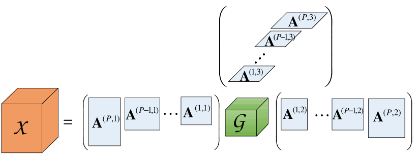
Figure 1: Visualization of the nested Tucker model.

III-D Block PARALIND/CONFAC models

In some applications, the data tensor ${\mathcal{X}}\in{\mathbb{C}}^{{I_{1}}\times{\cdots}\times{I_{N}}}$ is written as a sum of $P$ sub-tensors ${\mathcal{X}}^{(p)}$, each sub-tensor admitting a tensor model with a possibly different structure. So, we can define a block-PARALIND/CONFAC model as

$${\mathcal{X}} = \sum\limits_{p=1}^{P}{\mathcal{X}}^{(p)},$$ (68)

$${\mathcal{X}}^{(p)} = {\mathcal{G}}^{(p)}{\times}^{N}_{n=1}{\mathbf{A}}^{(p,n)},$$ (69)

$${\mathcal{G}}^{(p)} = {{\mathcal{I}}}_{N,R^{(p)}}\,{\times}^{N}_{n=1}{\mathbf{\Phi}}^{(p,n)},$$

where ${\mathbf{A}}^{(p,n)}\in{\mathbb{C}}^{{I_{n}}\times{R^{(p,n)}}}$, ${\mathbf{\Phi}}^{(p,n)}\in{\mathbb{C}}^{{R^{(p,n)}}\times{R^{(p)}}}$, and ${\mathcal{G}}^{(p)}\in{\mathbb{C}}^{{R^{(p,1)}}\times{\cdots}\times{R^{(p,N)}}}$ are the mode-$n$ factor matrix, the mode-$n$ constraint/allocation matrix, and the core tensor of the PARALIND/CONFAC model of the $p^{th}$ sub-tensor, respectively. The matrix representation (67) then becomes

$${\mathbf{X}}_{\mathds{S}_{1};\mathds{S}_{2}}=\sum\limits_{p=1}^{P}\left(\underset{n\in\mathds{S}_{1}}{\otimes}{\mathbf{A}}^{(p,n)}\right)\left(\underset{n\in\mathds{S}_{1}}{\diamond}{\mathbf{\Phi}}^{(p,n)}\right)\left(\underset{n\in\mathds{S}_{2}}{\diamond}{\mathbf{\Phi}}^{(p,n)}\right)^{T}\left(\underset{n\in\mathds{S}_{2}}{\otimes}{\mathbf{A}}^{(p,n)}\right)^{T}.$$ (70)

Defining the following block partitioned matrices

$${\mathbf{A}}^{(n)}=\left[\begin{array}[]{ccc}{\mathbf{A}}^{(1,n)}\cdots{\mathbf{A}}^{(P,n)}\end{array}\right]\in{\mathbb{C}}^{{I_{n}}\times{R^{(n)}}}$$ (72)

where $R^{(n)}=\sum\limits_{p=1}^{P}R^{(p,n)}$, Eq. (70) can be rewritten in the following more compact form

$${\mathbf{X}}_{\mathds{S}_{1};\mathds{S}_{2}}=\left(\underset{n\in\mathds{S}_{1}}{{\otimes}_{b}}{\mathbf{A}}^{(n)}\right){\mathbf{G}}_{\mathds{S}_{1};\mathds{S}_{2}}\left(\underset{n\in\mathds{S}_{2}}{{\otimes}_{b}}{\mathbf{A}}^{(n)}\right)^{T}$$

where ${\otimes}_{b}$ denotes the block-wise Kronecker product defined as

$${\mathbf{A}}^{(n)}{\otimes}_{b}{\mathbf{A}}^{(q)}=\left[\begin{array}[]{ccc}{\mathbf{A}}^{(1,n)}\otimes{\mathbf{A}}^{(1,q)}\cdots{\mathbf{A}}^{(P,n)}\otimes{\mathbf{A}}^{(P,q)}\end{array}\right]$$ (74)

${\mathbf{A}}^{(q)}$ being partitioned in $P$ blocks as in (72), and

$${\mathbf{G}}_{\mathds{S}_{1};\mathds{S}_{2}} = bdiag({\mathbf{G}}_{\mathds{S}_{1};\mathds{S}_{2}}^{(1)}\cdots{\mathbf{G}}_{\mathds{S}_{1};\mathds{S}_{2}}^{(P)})\in{\mathbb{C}}^{{J_{1}}\times{J_{2}}}$$

$${\mathbf{G}}_{\mathds{S}_{1};\mathds{S}_{2}}^{(p)} = \left(\underset{n\in\mathds{S}_{1}}{{\diamond}_{b}}{\mathbf{\Phi}}^{(p,n)}\right)\left(\underset{n\in\mathds{S}_{2}}{{\diamond}_{b}}{\mathbf{\Phi}}^{(p,n)}\right)^{T}\in{\mathbb{C}}^{{J_{1}^{(p)}}\times{J_{2}^{(p)}}}$$

where ${\diamond}_{b}$ denotes the block-wise Khatri-Rao product defined in the same way as the block-wise Kronecker product, with $J_{n_{1}}=\sum\limits_{p=1}^{P}{J_{n_{1}}^{(p)}}$ and $J_{n_{1}}^{(p)}=\underset{n\in\mathds{S}_{n_{1}}}{\prod}R^{(p,n)}$ for $n_{1}=1\,\textrm{and}\,\,2$.

In the case of a block PARAFAC model, Eq. (69) is replaced by

$${\mathcal{X}}^{(p)}={\mathcal{I}}_{N,R^{(p)}}{\times}^{N}_{n=1}{\mathbf{A}}^{(p,n)}\,\,\,\textrm{with}\,\,\,{\mathbf{A}}^{(p,n)}\in{\mathbb{C}}^{{I_{n}}\times{R^{(p)}}}$$

and the matrix representation (49) then becomes

$${\mathbf{X}}_{\mathds{S}_{1};\mathds{S}_{2}}=\left(\underset{n\in\mathds{S}_{1}}{{\diamond}_{b}}{\mathbf{A}}^{(n)}\right)\left(\underset{n\in\mathds{S}_{2}}{{\diamond}_{b}}{\mathbf{A}}^{(n)}\right)^{T}$$

with ${\mathbf{A}}^{(n)}=\left[\begin{array}[]{ccc}{\mathbf{A}}^{(1,n)}\cdots{\mathbf{A}}^{(P,n)}\end{array}\right]\in{\mathbb{C}}^{{I_{n}}\times{R}}$, and $R=\sum\limits_{p=1}^{P}{R^{(p)}}$. Block constrained PARAFAC models were used in [70], [71], [72] for modeling different types of multiuser wireless communication systems. Block constrained Tucker models were used for space-time multiplexing MIMO-OFDM systems [73], and for blind beamforming [74]. In these applications, the symbol matrix factor is in Toeplitz or block-Toeplitz form.

The block tensor model defined by Eq. (68)-(69) can be viewed as a generalization of the block term decomposition introduced in [76] for third-order tensors ${\mathcal{X}}\in{\mathbb{C}}^{{I}\times{J}\times{K}}$ that are decomposed into a sum of $P$ Tucker models of rank-$(L,M,N)$, which corresponds to the particular case where all the factor matrices are full column rank, with ${\mathbf{A}}^{(p,1)}\in{\mathbb{C}}^{{I}\times{L}}$, ${\mathbf{A}}^{(p,2)}\in{\mathbb{C}}^{{J}\times{M}}$, and ${\mathbf{A}}^{(p,3)}\in{\mathbb{C}}^{{K}\times{N}}$, for $p=1,\cdots,P$, and ${\mathcal{G}}\in{\mathbb{C}}^{{L}\times{M}\times{N}}$, and each sub-tensor ${\mathcal{X}}^{(p)}$ is decomposed by means of its HOSVD.

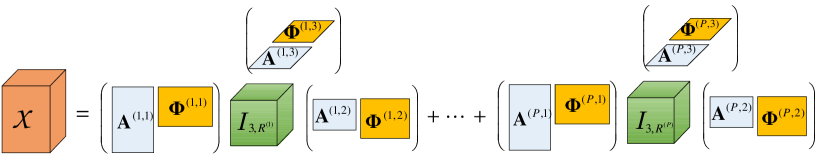
Figure 2: Visualization of the block PARALIND/CONFAC model.

This figure is to be compared with Figure 5 in [77] representing a block term decomposition of a third-order tensor into rank-$(L_{p},M_{p},N_{p})$ terms, when each term has a PARALIND/CONFAC structure.

III-E PARALIND/CONFAC-$(N_{1},N)$ models

Now, we introduce a variant of PARALIND/CONFAC models that we shall call PARALIND/CONFAC-$(N_{1},N)$ models. This variant corresponds to PARALIND/CONFAC models (65) with only $N_{1}$ constrained matrix factors, which implies $R_{n}=R$ and ${\mathbf{A}}^{(n)}\in{\mathbb{C}}^{{I_{n}}\times{R}}$ for $n=N_{1}+1,\cdots,N$

$${\mathcal{X}}={{\mathcal{I}}}_{N,R}\,{\times}^{N_{1}}_{n=1}({\mathbf{A}}^{(n)}{\mathbf{\Phi}}^{(n)})\,{\times}^{N}_{n=N_{1}+1}{\mathbf{A}}^{(n)}.$$ (75)

In [78], a block PARALIND/CONFAC-(2,3) model that can be deduced from (75), was used for modeling uplink multiple-antenna code-division multiple-access (CDMA) multiuser systems.

The block term decomposition (BTD) in rank-$(1,L_{p},L_{p})$ terms of a third-order tensor ${\mathcal{X}}\in{\mathbb{C}}^{{I}\times{J}\times{K}}$, which is compared to a third-order PARATREE model in [75], can also be viewed as a particular CONFAC-(1,3) model. Indeed, such a decomposition can be written as [79]

$${\mathcal{X}}=\sum\limits_{p=1}^{P}{\mathbf{a}}_{p}\circ({\mathbf{B}}_{p}{\mathbf{C}}_{p}^{T})$$ (76)

where the matrices ${\mathbf{B}}_{p}\in{\mathbb{C}}^{{J}\times{L_{p}}}$ and ${\mathbf{C}}_{p}\in{\mathbb{C}}^{{K}\times{L_{p}}}$ are rank-$L_{p}$, and ${\mathbf{a}}_{p}\in{\mathbb{C}}^{{I}\times{1}}$. Defining ${\mathbf{B}}=[{\mathbf{B}}_{1}\cdots{\mathbf{B}}_{P}]\in{\mathbb{C}}^{{J}\times{R}}$, ${\mathbf{C}}=[{\mathbf{C}}_{1}\cdots{\mathbf{C}}_{P}]\in{\mathbb{C}}^{{K}\times{R}}$, and ${\mathbf{A}}=[{\mathbf{a}}_{1}\cdots{\mathbf{a}}_{P}]\in{\mathbb{C}}^{{I}\times{P}}$, with $R=\sum\limits_{p=1}^{P}L_{p}$, it is easy to verify that the BTD (76) can be rewritten as the following CONFAC-(1,3) model

$${\mathcal{X}}={\mathcal{I}}_{3,R}\times_{1}{\mathbf{A}}{\bf{\Phi}}\times_{2}{\mathbf{B}}\times_{3}{\mathbf{C}}$$ (77)

with the constraint matrix ${\mathbf{\Phi}}=\left[\begin{array}[]{ccc}{\mathbf{1}}_{L_{1}}^{T}&&\\ &\ddots&\\ &&{\mathbf{1}}_{L_{P}}^{T}\end{array}\right]\in{\mathbb{C}}^{{P}\times{R}}$.

III-F PARATUCK models

A PARATUCK-$(N_{1},N)$ model for a $N^{th}$-order tensor ${\mathcal{X}}\in{\mathbb{C}}^{{I_{1}}\times{\cdots}\times{I_{N}}}$, with $N>N_{1}$, is defined in scalar form as follows [66], [67]

$$x_{i_{1},\cdots,i_{N_{1}+1},\cdots,i_{N}}=\sum\limits_{r_{1}=1}^{R_{1}}\cdots\sum\limits_{r_{N_{1}}=1}^{R_{N_{1}}}c_{r_{1},\cdots,r_{N_{1}},i_{{N_{1}}+2},\cdots,i_{N}}\prod\limits_{n=1}^{N_{1}}a^{(n)}_{i_{n},r_{n}}\phi^{(n)}_{r_{n},i_{{N_{1}}+1}}$$ (78)

where $a^{(n)}_{i_{n},r_{n}}$, and $\phi^{(n)}_{r_{n},i_{{N_{1}}+1}}$ are entries of the factor matrix ${\mathbf{A}}^{(n)}\in{\mathbb{C}}^{{I_{n}}\times{R_{n}}}$ and of the interaction/allocation matrix ${\mathbf{\Phi}}^{(n)}\in{\mathbb{C}}^{{R_{n}}\times{I_{{N_{1}}+1}}},\,\forall n=1,\cdots,N_{1}$, respectively, and ${\mathcal{C}}\in{\mathbb{C}}^{{R_{1}\times\cdots}\times{R_{N_{1}}\times I_{N_{1}+2}\times\cdots}\times{I_{N}}}$ is the $(N-1)^{th}$-order input tensor. Defining the core tensor ${\mathcal{G}}\in{\mathbb{C}}^{{R_{1}\times\cdots}\times{R_{N_{1}}\times I_{N_{1}+1}\times\cdots}\times{I_{N}}}$ element-wise as

$$g_{r_{1},\cdots,r_{N_{1}},i_{{N_{1}}+1},\cdots,i_{N}} = c_{r_{1},\cdots,r_{N_{1}},i_{{N_{1}}+2},\cdots,i_{N}}\prod\limits_{n=1}^{N_{1}}\phi^{(n)}_{r_{n},i_{{N_{1}}+1}}$$

the PARATUCK-$(N_{1},N)$ model can be rewritten as a Tucker-$(N_{1},N)$ model (38)-(39).

Defining the allocation/interaction tensor ${\mathcal{F}}\in{\mathbb{C}}^{{R_{1}\times\cdots}\times{R_{N_{1}}}\times{I_{N_{1}+1}}}$ of order $N_{1}+1$, such as

$$f_{r_{1},\cdots,r_{N_{1}},i_{N_{1}+1}}=\prod\limits_{n=1}^{N_{1}}\phi^{(n)}_{r_{n},i_{N_{1}+1}}.$$ (79)

the core tensor ${\mathcal{G}}$ can then be written as the Hadamard product of the tensors ${\mathcal{C}}$ and ${\mathcal{F}}$ along their first $N_{1}$ modes

$${\mathcal{G}}=\,{\mathcal{C}}\,\underset{\{r_{1},\cdots,r_{N_{1}}\}}{\odot}\,{\mathcal{F}}.$$ (80)

Remarks

• The PARATUCK-$(N1,N)$ model can be interpreted as the transformation of the input tensor ${\mathcal{C}}$ via its multiplication by the factor matrices ${\mathbf{A}}^{(n)},n=1,\cdots,N_{1}$, along its first $N_{1}$ modes, combined with a mode-$n$ resource allocation $(n=1,\cdots,N_{1})$ relatively to the mode-$(N_{1}+1)$ of the transformed tensor ${\mathcal{X}}$, by means of the allocation matrices ${\mathbf{\Phi}}^{(n)}$.

• In telecommunications applications, the output modes will be called diversity modes because they correspond to time, space and frequency diversities, whereas the input modes are associated with resources like transmit antennas, codes, and data streams. For these applications, the matrices ${\mathbf{\Phi}}^{(n)}$ are formed with 0’s and 1’s, and they can be interpreted as allocation matrices used for allocating some resources $r_{n}$ to the output mode-$(N_{1}+1)$. Another way to take resource allocations into account consists in replacing the $N_{1}$ allocation matrices ${\mathbf{\Phi}}^{(n)}$ by the $(N_{1}+1)^{th}$-order allocation tensor ${\mathcal{F}}\in{\mathbb{C}}^{{R_{1}\times\cdots}\times{R_{N_{1}}}\times{I_{N_{1}+1}}}$ defined in (79).

• Special cases:

  • For $N_{1}=2$ and $N=3$, we obtain the standard PARATUCK-2 model introduced in [59]. Eq. (78) then becomes

    $$x_{i_{1},i_{2},i_{3}}=\sum\limits_{r_{1}=1}^{R_{1}}\sum\limits_{r_{2}=1}^{R_{2}}c_{r_{1},r_{2}}a^{(1)}_{i_{1},r_{1}}a^{(2)}_{i_{2},r_{2}}\phi^{(1)}_{r_{1},i_{3}}\phi^{(2)}_{r_{2},i_{3}}$$ (81)

    The allocation tensor ${\mathcal{F}}$ defined in (79) can be rewritten as

    $$f_{r_{1},r_{2},i_{3}}=\phi^{(1)}_{r_{1},i_{3}}\phi^{(2)}_{r_{2},i_{3}}=\sum\limits_{j=1}^{I_{3}}\phi^{(1)}_{r_{1},j}\phi^{(2)}_{r_{2},j}\delta_{i_{3},j}$$ (82)

    which corresponds to a PARAFAC model with matrix factors ($\bf{\Phi}^{(1)},\bf{\Phi}^{(2)},{\mathbf{I}}_{I_{3}}$). The PARATUCK-2 model (81) can then be viewed as a Tucker-2 model ${\mathcal{X}}={\mathcal{G}}{\times}_{1}{\mathbf{A}}^{(1)}{\times}_{2}{\mathbf{A}}^{(2)}$ with the core tensor ${\mathcal{G}}\in{\mathbb{C}}^{{R_{1}}\times{R_{2}}\times{I_{3}}}$ given by the Hadamard product of ${\mathbf{C}}\in{\mathbb{C}}^{{R_{1}}\times{R_{2}}}$ and ${\mathcal{F}}\in{\mathbb{C}}^{{R_{1}}\times{R_{2}}\times{I_{3}}}$ along their common modes $\{r_{1},r_{2}\}$

    $${\mathcal{G}}={\mathbf{C}}\underset{\{r_{1},r_{2}\}}{\odot}{\mathcal{F}}$$

    This combination of a Tucker-2 model for ${\mathcal{X}}$ with a PARAFAC model for ${\mathcal{F}}$ gave rise to the name PARATUCK-2. The constraint matrices ($\bf{\Phi}^{(1)},\bf{\Phi}^{(2)}$) define interactions between columns of the factor matrices (${\mathbf{A}}^{(1)},{\mathbf{A}}^{(2)}$), along the mode-3 of ${\mathcal{X}}$, while the matrix ${\mathbf{C}}$ contains the weights of these interactions.

  • For $N_{1}=2$ and $N=4$, we obtain the PARATUCK-(2,4) model introduced in [66]

    $$x_{i_{1},i_{2},i_{3},i_{4}}=\sum\limits_{r_{1}=1}^{R_{1}}\sum\limits_{r_{2}=1}^{R_{2}}c_{r_{1},r_{2},i_{4}}a^{(1)}_{i_{1},r_{1}}a^{(2)}_{i_{2},r_{2}}\phi^{(1)}_{r_{1},i_{3}}\phi^{(2)}_{r_{2},i_{3}}$$ (83)

    As for the PARATUCK-2 model, the PARATUCK-(2,4) can be viewed as a combination of a Tucker-(2,4) model for ${\mathcal{X}}={\mathcal{G}}{\times}_{1}{\mathbf{A}}^{(1)}{\times}_{2}{\mathbf{A}}^{(2)}\in{\mathbb{C}}^{{I_{1}}\times{I_{2}}\times{I_{3}\times I_{4}}}$ with a core tensor ${\mathcal{G}}\in{\mathbb{C}}^{{R_{1}}\times{R_{2}}\times{I_{3}\times I_{4}}}$ given by the Hadamard product of the tensors ${\mathcal{C}}\in{\mathbb{C}}^{{R_{1}}\times{R_{2}}\times{I_{4}}}$ and ${\mathcal{F}}\in{\mathbb{C}}^{{R_{1}}\times{R_{2}}\times{I_{3}}}$ along their common modes $\{r_{1},r_{2}\}$

    $${\mathcal{G}}={\mathcal{C}}\underset{\{r_{1},r_{2}\}}{\odot}{\mathcal{F}}$$

    with the same allocation tensor ${\mathcal{F}}$ defined in (82).

III-G Rewriting of PARATUCK models as Constrained PARAFAC Models

This rewriting of PARATUCK models as constrained PARAFAC models can be used to deduce both matrix unfoldings by means of the general formula (49), and sufficient conditions for essential uniqueness of such PARATUCK models, as will be shown in Section IV.

III-G1 Link between PARATUCK-(2,4) and constrained PARAFAC-4 models

We now establish the link between the PARATUCK-(2,4) model (83) and the fourth-order constrained PARAFAC model

$$x_{i_{1},i_{2},i_{3},i_{4}}=\sum\limits_{r=1}^{R}{a}_{i_{1},r}{b}_{i_{2},r}{f}_{i_{3},r}{d}_{i_{4},r}\quad\textrm{with}\quad R=R_{1}R_{2}$$ (84)

whose matrix factors (${{\mathbf{A}}}\in{\mathbb{C}}^{{I_{1}}\times{R}}$, ${{\mathbf{B}}}\in{\mathbb{C}}^{{I_{2}}\times{R}}$, ${{\mathbf{F}}}\in{\mathbb{C}}^{{I_{3}}\times{R}}$, ${{\mathbf{D}}}\in{\mathbb{C}}^{{I_{4}}\times{R}}$), and constraint matrices (${\mathbf{\Psi}}^{(1)},{\mathbf{\Psi}}^{(2)}$) acting on the original factors (${\mathbf{A}}^{(1)},{\mathbf{A}}^{(2)}$), are given by

$${{\mathbf{A}}}={\mathbf{A}}^{(1)}{\mathbf{\Psi}}^{(1)},\quad{{\mathbf{B}}}={\mathbf{A}}^{(2)}{\mathbf{\Psi}}^{(2)},\quad{{\mathbf{F}}}=({\mathbf{\Phi}}^{(1)}\diamond{\mathbf{\Phi}}^{(2)})^{T},\quad{{\mathbf{D}}}={\mathbf{C}}_{I_{4}\times R_{1}R_{2}}$$ (85)

$${\mathbf{\Psi}}^{(1)}={\mathbf{I}}_{R_{1}}\otimes{{\mathbf{1}}}^{T}_{R_{2}}\in{\mathbb{C}}^{{R_{1}}\times{R_{1}R_{2}}},\quad{\mathbf{\Psi}}^{(2)}={{\mathbf{1}}}^{T}_{R_{1}}\otimes{\mathbf{I}}_{R_{2}}\in{\mathbb{C}}^{{R_{2}}\times{R_{1}R_{2}}}$$ (86)

where ${\mathbf{C}}_{I_{4}\times R_{1}R_{2}}\in{\mathbb{C}}^{{I_{4}}\times{R_{1}R_{2}}}$ is a mode-3 unfolded matrix of the tensor ${\mathcal{C}}\in{\mathbb{C}}^{{R_{1}}\times{R_{2}}\times{I_{4}}}$.

Proof:

See the Appendix. ∎

Remarks

• Application of the formula (50) to the constrained PARAFAC model (84), with the matrix factors $({{\mathbf{A}}},{{\mathbf{B}}},{{\mathbf{F}}},{{\mathbf{D}}})=({\mathbf{A}}^{(1)}{\mathbf{\Psi}}^{(1)},{\mathbf{A}}^{(2)}{\mathbf{\Psi}}^{(2)},({\mathbf{\Phi}}^{(1)}\diamond{\mathbf{\Phi}}^{(2)})^{T},{\mathbf{C}}_{I_{4}\times R_{1}R_{2}})$, gives the following flat modes-1 and -2 matrix unfoldings for the PARATUCK-(2,4) model (83)

  $${\mathbf{X}}_{I_{1}\times I_{2}I_{3}I_{4}} = {\mathbf{A}}^{(1)}{\mathbf{\Psi}}^{(1)}({\mathbf{A}}^{(2)}{\mathbf{\Psi}}^{(2)}\diamond{\mathbf{F}}\diamond{\mathbf{D}})^{T}\in{\mathbb{C}}^{{I_{1}}\times{I_{2}I_{3}I_{4}}},$$

  $${\mathbf{X}}_{I_{2}\times I_{3}I_{4}I_{1}} = {\mathbf{A}}^{(2)}{\mathbf{\Psi}}^{(2)}({\mathbf{F}}\diamond{\mathbf{D}}\diamond{\mathbf{A}}^{(1)}{\mathbf{\Psi}}^{(1)})^{T}\in{\mathbb{C}}^{{I_{2}}\times{I_{3}I_{4}I_{1}}}.$$

• The constrained PARAFAC-4 model (84)-(86) can be written in mode-$n$ products notation as

  $${\mathcal{X}}={\mathcal{I}}_{4,R}{\times}_{1}{\mathbf{A}}^{(1)}{\mathbf{\Psi}}^{(1)}{\times}_{2}{\mathbf{A}}^{(2)}{\mathbf{\Psi}}^{(2)}{\times}_{3}{{\mathbf{F}}}{\times}_{4}{{\mathbf{D}}}.$$ (87)

  Defining the core tensor ${\mathcal{G}}\in{\mathbb{C}}^{{R_{1}}\times{R_{2}}\times{I_{3}\times I_{4}}}$ as

  $${\mathcal{G}}={\mathcal{I}}_{4,R}{\times}_{1}{\mathbf{\Psi}}^{(1)}{\times}_{2}{\mathbf{\Psi}}^{(2)}{\times}_{3}{{\mathbf{F}}}{\times}_{4}{{\mathbf{D}}}$$ (88)

  the constrained PARAFAC-4 model can also be viewed as the following Tucker-(2,4) model

  $${\mathcal{X}}={\mathcal{G}}{\times}_{1}{\mathbf{A}}^{(1)}{\times}_{2}{\mathbf{A}}^{(2)}.$$ (89)

  It can also be viewed as a CONFAC-(2,4) model with matrix factors $({\mathbf{A}}^{(1)},{\mathbf{A}}^{(2)},{\mathbf{F}},{\mathbf{D}})$, and constraint matrices ${\mathbf{\Psi}}^{(1)}$ and ${\mathbf{\Psi}}^{(2)}$ defined in (86).

• Choosing $\mathds{S}_{1}=\{i_{1},i_{2}\}$ and $\mathds{S}_{2}=\{i_{3},i_{4}\}$, the matrix unfolding (49) of the PARAFAC model (87) is given by

  $${\mathbf{X}}_{I_{1}I_{2}\times I_{3}I_{4}} = ({\mathbf{A}}^{(1)}{\mathbf{\Psi}}^{(1)}\diamond{\mathbf{A}}^{(2)}{\mathbf{\Psi}}^{(2)})\big{(}{\mathbf{F}}\diamond{\mathbf{D}}\big{)}^{T}$$ (90)

  $$= ({\mathbf{A}}^{(1)}\otimes{\mathbf{A}}^{(2)})\big{(}{\mathbf{F}}\diamond{\mathbf{D}}\big{)}^{T}\in{\mathbb{C}}^{{I_{1}I_{2}}\times{I_{3}I_{4}}}$$

  Proof:

  Using the identity (133) gives

  $${\mathbf{A}}^{(1)}{\mathbf{\Psi}}^{(1)}\diamond{\mathbf{A}}^{(2)}{\mathbf{\Psi}}^{(2)}=({\mathbf{A}}^{(1)}\otimes{\mathbf{A}}^{(2)})({\mathbf{\Psi}}^{(1)}\diamond{\mathbf{\Psi}}^{(2)})$$ (91)

  Replacing ${\mathbf{\Psi}}^{(1)}$ and ${\mathbf{\Psi}}^{(2)}$ by their expressions (142) and (143) leads to

  $${\mathbf{\Psi}}^{(1)}\diamond{\mathbf{\Psi}}^{(2)} = ({\mathbf{I}}_{R_{1}}\otimes{{\mathbf{1}}}^{T}_{R_{2}})\diamond({{\mathbf{1}}}^{T}_{R_{1}}\otimes{\mathbf{I}}_{R_{2}})$$ (95)

  $$= \underset{R_{1}\,\,\textrm{blocks}}{\underbrace{\left[\begin{array}[]{ccc}{\mathbf{I}}_{R_{2}}&&\\ &\ddots&\\ &&{\mathbf{I}}_{R_{2}}\end{array}\right]}}={\mathbf{I}}_{R_{1}R_{2}}$$

  which implies

  $${\mathbf{A}}^{(1)}{\mathbf{\Psi}}^{(1)}\diamond{\mathbf{A}}^{(2)}{\mathbf{\Psi}}^{(2)}={\mathbf{A}}^{(1)}\otimes{\mathbf{A}}^{(2)},$$ (96)

  and consequently Eq. (90) can be deduced.
  This equation can also be obtained from the equivalent Tucker-(2,4) model (88)-(89) as

  $${\mathbf{X}}_{I_{1}I_{2}\times I_{3}I_{4}}=({\mathbf{A}}^{(1)}\otimes{\mathbf{A}}^{(2)}){\mathbf{G}}_{R_{1}R_{2}\times I_{3}I_{4}}$$ (97)

  with

  $${\mathbf{G}}_{R_{1}R_{2}\times I_{3}I_{4}}=({\mathbf{\Psi}}^{(1)}\diamond{\mathbf{\Psi}}^{(2)})({\mathbf{F}}\diamond{\mathbf{D}})^{T}$$

  Using the identity (96), we obtain

  $${\mathbf{G}}_{R_{1}R_{2}\times I_{3}I_{4}}=({\mathbf{F}}\diamond{\mathbf{D}})^{T}$$ (98)

  and replacing ${\mathbf{G}}_{R_{1}R_{2}\times I_{3}I_{4}}$ by its expression (98) into (97) gives (90).

  ∎

  When the allocation matrices (${\mathbf{\Phi}}^{(1)}$, ${\mathbf{\Phi}}^{(2)}$) and the input tensor ${\mathcal{C}}$ are known, the matrix factors $({\mathbf{A}}^{(1)},{\mathbf{A}}^{(2)})$ can be estimated through the LS estimation of their Kronecker product using the matrix unfolding (90).

• The product $\phi^{(1)}_{r_{1},i_{3}}\phi^{(2)}_{r_{2},i_{3}}$ in (83) can be replaced by $f_{i_{3},r_{1},r_{2}}$ , which amounts to replace the allocation matrices ${\mathbf{\Phi}}^{(1)}$ and ${\mathbf{\Phi}}^{(2)}$ by the third-order allocation tensor ${\mathcal{F}}\in{\mathbb{C}}^{{I_{3}}\times{R_{1}}\times{R_{2}}}$, the matrix ${{\mathbf{F}}}=({\mathbf{\Phi}}^{(1)}\diamond{\mathbf{\Phi}}^{(2)})^{T}\in{\mathbb{C}}^{{I_{3}}\times{R_{1}R_{2}}}$ being equivalent to ${\mathbf{F}}_{I_{3}\times R_{1}R_{2}}\in{\mathbb{C}}^{{I_{3}}\times{R_{1}R_{2}}}$, i.e. a mode-1 flat matrix unfolding of the allocation tensor ${\mathcal{F}}$.

III-G2 Link between PARATUCK-2 and constrained PARAFAC-3 models

By proceeding in the same way as for the PARATUCK-(2,4) model, it is easy to show that the PARATUCK-2 model (81) is equivalent to a third-order constrained PARAFAC model whose matrix factors ${{\mathbf{A}}}\in{\mathbb{C}}^{{I_{1}}\times{R}}$, ${{\mathbf{B}}}\in{\mathbb{C}}^{{I_{2}}\times{R}}$, and ${{\mathbf{F}}}\in{\mathbb{C}}^{{I_{3}}\times{R}}$, with $R=R_{1}R_{2}$, are given by

$${{\mathbf{A}}}={\mathbf{A}}^{(1)}{\mathbf{\Psi}}^{(1)},\quad{{\mathbf{B}}}={\mathbf{A}}^{(2)}{\mathbf{\Psi}}^{(2)},\quad{{\mathbf{F}}}=({\mathbf{\Phi}}^{(1)}\diamond{\mathbf{\Phi}}^{(2)})^{T}diag(\textrm{vec}({\mathbf{C}}^{T}))$$ (99)

with the same constraint matrices ${\mathbf{\Psi}}^{(1)}$ and ${\mathbf{\Psi}}^{(2)}$ defined in (86). By analogy with the PARATUCK-(2,4) model, Eq. (87), (89), and (90) become for the PARATUCK-2 model

$${\mathcal{X}} = {\mathcal{I}}_{3,R}{\times}_{1}{\mathbf{A}}^{(1)}{\mathbf{\Psi}}^{(1)}{\times}_{2}{\mathbf{A}}^{(2)}{\mathbf{\Psi}}^{(2)}{\times}_{3}{{\mathbf{F}}}$$ (100)

$$= {\mathcal{G}}{\times}_{1}{\mathbf{A}}^{(1)}{\times}_{2}{\mathbf{A}}^{(2)}$$

with the core tensor ${\mathcal{G}}\in{\mathbb{C}}^{{R_{1}}\times{R_{2}}\times{I_{3}}}$ defined as

$${\mathcal{G}}={\mathcal{I}}_{3,R}{\times}_{1}{\mathbf{\Psi}}^{(1)}{\times}_{2}{\mathbf{\Psi}}^{(2)}{\times}_{3}{{\mathbf{F}}},$$ (101)

and

$${\mathbf{X}}_{I_{1}I_{2}\times I_{3}}=({\mathbf{A}}^{(1)}\otimes{\mathbf{A}}^{(2)}){{\mathbf{F}}}^{T}\in{\mathbb{C}}^{{I_{1}I_{2}}\times{I_{3}}}.$$

Remarks

• Eq. (100) and (101) allow interpreting the PARATUCK-2 model as a Tucker-(2,3) model, defined in (40)-(41). If we choose $c_{r_{1},r_{2}}=1,\forall r_{k}=1,\cdots,R_{k}$, for $k$=1 and 2, and define the allocation tensor ${\mathcal{F}}\in{\mathbb{C}}^{{R_{1}}\times{R_{2}}\times{I_{3}}}$ such as $f_{r_{1},r_{2},i_{3}}=\phi^{(1)}_{r_{1},i_{3}}\phi^{(2)}_{r_{2},i_{3}}$, the PARATUCK-2 model (81) becomes the following Tucker-(2,3) model

  $$x_{i_{1},i_{2},i_{3}}=\sum\limits_{r_{1}=1}^{R_{1}}\sum\limits_{r_{2}=1}^{R_{2}}f_{r_{1},r_{2},i_{3}}a^{(1)}_{i_{1},r_{1}}a^{(2)}_{i_{2},r_{2}}$$

  and the associated constrained PARAFAC-3 model can be deduced from (99)

  $${{\mathbf{A}}}={\mathbf{A}}^{(1)}{\mathbf{\Psi}}^{(1)},\quad{{\mathbf{B}}}={\mathbf{A}}^{(2)}{\mathbf{\Psi}}^{(2)},\quad{{\mathbf{F}}}={\mathbf{F}}_{I_{3}\times R_{1}R_{2}}=({\mathbf{\Phi}}^{(1)}\diamond{\mathbf{\Phi}}^{(2)})^{T}$$

  with the same constraint matrices ${\mathbf{\Psi}}^{(1)}$ and ${\mathbf{\Psi}}^{(2)}$ as those defined in (86). A block Tucker-(2,3) model transformed into a block constrained PARAFAC-3 model was used in [72] for modeling in an unified way three multiuser wireless communication systems.

• Now, we show the equivalence of the expressions (101) and (80) of the core tensor. Applying the formula (50) to the PARAFAC model (101) gives

  $${\mathbf{G}}_{I_{3}\times R_{1}R_{2}}=({\mathbf{\Phi}}^{(1)}\diamond{\mathbf{\Phi}}^{(2)})^{T}diag(\textrm{vec}({\mathbf{C}}^{T}))({\mathbf{\Psi}}^{(1)}\diamond{\mathbf{\Psi}}^{(2)})^{T}.$$ (102)

  Using the identity (96) in Eq. (102) gives ${\mathbf{G}}_{I_{3}\times R_{1}R_{2}}=({\mathbf{\Phi}}^{(1)}\diamond{\mathbf{\Phi}}^{(2)})^{T}diag(\textrm{vec}({\mathbf{C}}^{T}))$.

  For the formula (80), with $N=3$ and $N_{1}=2$, we have

  $${\mathcal{G}}={\mathcal{F}}\underset{\{r_{1},r_{2}\}}{\odot}{\mathbf{C}}$$

  or equivalently in terms of matrix Hadamard product

  $${\mathbf{G}}_{I_{3}\times R_{1}R_{2}}={\mathbf{F}}_{I_{3}\times R_{1}R_{2}}\odot{\mathbf{1}}_{I_{3}}{\mathbf{c}}_{1\times R_{1}R_{2}}$$

  with ${\mathbf{F}}_{I_{3}\times R_{1}R_{2}}=({\mathbf{\Phi}}^{(1)}\diamond{\mathbf{\Phi}}^{(2)})^{T}$, and ${\mathbf{c}}_{1\times R_{1}R_{2}}=\textrm{vec}^{T}({{\mathbf{C}}}^{T})$, which gives

  $${\mathbf{G}}_{I_{3}\times R_{1}R_{2}}={\mathbf{F}}_{I_{3}\times R_{1}R_{2}}\odot\left[\begin{array}[]{c}\textrm{vec}^{T}({{\mathbf{C}}}^{T})\\ \vdots\\ \textrm{vec}^{T}({{\mathbf{C}}}^{T})\end{array}\right]\Bigg{\}}{\mathbf{I}}_{3}\,\textrm{rows}$$ (105)

  and consequently ${\mathbf{G}}_{I_{3}\times R_{1}R_{2}}=({\mathbf{\Phi}}^{(1)}\diamond{\mathbf{\Phi}}^{(2)})^{T}diag(\textrm{vec}({\mathbf{C}}^{T}))$, showing the equivalence of the two core tensor expressions (101) and (80).

III-G3 Link between PARATUCK-$(N-2,N)$ and constrained PARAFAC-$N$ models

Let us consider the PARATUCK-$(N_{1},N)$ model (78) in the case $N_{1}=N-2$

$$x_{i_{1},\cdots,i_{N_{1}+1},\cdots,i_{N}}=\sum\limits_{r_{1}=1}^{R_{1}}\cdots\sum\limits_{r_{N_{1}}=1}^{R_{N_{1}}}c_{r_{1},\cdots,r_{N_{1}},i_{N}}\prod\limits_{n=1}^{N_{1}}a^{(n)}_{i_{n},r_{n}}\phi^{(n)}_{r_{n},i_{{N_{1}}+1}}$$ (106)

and let us define the change of variables $r=r_{N_{1}}+\sum\limits_{n=1}^{{N_{1}}-1}(r_{n}-1)\prod\limits_{i=n+1}^{N_{1}}R_{i}$ corresponding to a combination of the $N_{1}$ modes associated with the constraints/allocations. Eq. (106) can then be written as the following constrained PARAFAC-$N$ model

$$x_{i_{1},\cdots,i_{N}}=\sum\limits_{r=1}^{R}\prod\limits_{n=1}^{N}\bar{a}^{(n)}_{i_{n},r},\quad R=\prod\limits_{i=1}^{N_{1}}R_{i}$$ (107)

with the following matrix factors

$$\bar{{\mathbf{A}}}^{(n)}={\mathbf{A}}^{(n)}{\mathbf{\Psi}}^{(n)},\,n=1,\cdots,N_{1};\quad{{\mathbf{F}}}={\left(\overset{N}{\underset{n=1}{\diamond}}{\mathbf{\Phi}}^{(n)}\right)}^{T};\quad{{\mathbf{D}}}={\mathbf{C}}_{I_{N}\times R_{1}\cdots R_{N_{1}}},$$

where ${\mathbf{C}}_{I_{N}\times R_{1}\cdots R_{N_{1}}}\in{\mathbb{C}}^{{I_{N}}\times{R_{1}\cdots R_{N_{1}}}}$ is a mode-$(N_{1}+1)$ unfolded matrix of the tensor ${\mathcal{C}}\in{\mathbb{C}}^{{R_{1}\times\cdots}\times{R_{N_{1}}}\times{I_{N}}}$, and the constraint matrices are given in (144) as

$${\mathbf{\Psi}}^{(n)}={{\mathbf{1}}}^{T}_{R_{1}}\otimes\cdots\otimes{{\mathbf{1}}}^{T}_{R_{n-1}}\otimes{\mathbf{I}}_{R_{n}}\otimes{{\mathbf{1}}}^{T}_{R_{n+1}}\otimes\cdots\otimes{{\mathbf{1}}}^{T}_{R_{N}}\in{\mathbb{C}}^{{R_{n}}\times{R}},n=1,\cdots,N_{1}.$$

The constrained PARAFAC model (107) can also be written as a Tucker-$(N_{1},N)$ model (39) with the core tensor defined in (80), or, equivalently,

$${\mathcal{G}}={\mathcal{I}}_{N,R}{\times}_{n=1}^{N-2}{\mathbf{\Psi}}^{(n)}{\times}_{N-1}{{\mathbf{F}}}{\times}_{N}{{\mathbf{D}}}.$$

III-H Comparison of constrained tensor models

To conclude this presentation, we compare the so called CONFAC-$(N_{1},N)$ and PARATUCK-$(N_{1},N)$ constrained tensor models, introduced in this paper with a resource allocation point of view. Due to the PARAFAC structure (64) of the core tensor of CONFAC models, each element $x_{i_{1},\cdots,i_{N}}$ of the output tensor ${\mathcal{X}}$ is the sum of $R$ components as shown in (66). Moreover, due to the special structure of the allocation matrices ${\mathbf{\Phi}}^{(n)}$ whose the columns are unit vectors, each component $r$ is the result of a combination of $N$ resources, under the form of the product $\prod\limits_{n=1}^{N}a^{(n)}_{i_{n},r_{n}}$, the $N$ resources being fixed by the allocation matrices ${\mathbf{\Phi}}^{(n)}\in{\mathbb{C}}^{{R_{n}}\times{R}}$.

With the CONFAC-$(N_{1},N)$ model (75), each component $r$ is a combination of $N_{1}$ resources $(r_{1},\cdots,r_{N_{1}})$ determined by the allocation matrices ${\mathbf{\Phi}}^{(n)}\in{\mathbb{C}}^{{R_{n}}\times{R}}$ for $n=1,\cdots,N_{1}$.

There are two main differences between the PARATUCK-$(N_{1},N)$ models (78) and the CONFAC models (65). The first one is that the allocation matrices of PARATUCK models, formed with 0’s and 1’s, have not necessarily unit vectors as column vectors, which means that it is possible to allocate $\gamma_{n}=\sum\limits_{r_{n}=1}^{R_{n}}\phi^{(n)}_{r_{n},i_{N_{1}+1}}$ resources $r_{n}$ to the $(N_{1}+1)^{th}$-mode of the output tensor ${\mathcal{X}}$. The second one results from the interpretation of PARATUCK-$(N_{1},N)$ models as Tucker-$(N_{1},N)$ models, implying that each element $x_{i_{1},\cdots,i_{N}}$ of ${\mathcal{X}}$ is equal to the sum of $\sum\limits_{r_{1}=1}^{R_{1}}\cdots\sum\limits_{r_{N_{1}}=1}^{R_{N_{1}}}f_{r_{1},\cdots,r_{N_{1}},i_{{N_{1}}+1}}$ terms, where $f_{r_{1},\cdots,r_{N_{1}},i_{{N_{1}}+1}}$ is an entry of the allocation tensor ${\mathcal{F}}$ defined in (79), each term being a combination of resources under the form of products $\prod\limits_{n=1}^{N_{1}}a^{(n)}_{i_{n},r_{n}}$. Moreover, in telecommunication applications, the input tensor ${\mathcal{C}}$ can be used as a code tensor.

Another way to compare PARALIND/CONFAC and PARATUCK models is in terms of dependencies/interactions between their factor matrices. In the case of PARALIND/CONFAC models, as pointed out by Eq. (65), the constraint matrices act independently on each factor matrix, expliciting linear dependencies between columns of these matrices. For PARATUCK models, their writing as Tucker-$(N_{1},N)$ models with the core tensor defined in (80) allows to interpret the tensor ${\mathcal{F}}$ as an interaction tensor which defines interactions between $N_{1}$ factor matrices, the tensor ${\mathcal{C}}$ providing the strength of these interactions.

The main constrained PARAFAC models are summarized in Tables I and II.

TABLE I: Main tensor models

Models	Scalar writings	mode-$n$ product based writings
PARAFAC-3	$x_{i_{1},i_{2},i_{3}}=\sum\limits_{r}^{R}a^{(1)}_{i_{1},r}a^{(2)}_{i_{2},r}a^{(3)}_{i_{3},r}$	${\mathcal{X}}={\mathcal{I}}_{3,R}\times_{1}{\mathbf{A}}^{(1)}\times_{2}{\mathbf{A}}^{(2)}\times_{3}{\mathbf{A}}^{(3)}$
Tucker-3	$x_{i_{1},i_{2},i_{3}}=\sum\limits_{r_{1}=1}^{R_{1}}\sum\limits_{r_{2}=1}^{R_{2}}\sum\limits_{r_{3}=1}^{R_{3}}g_{r_{1},r_{2},r_{3}}a^{(1)}_{i_{1},r_{1}}a^{(2)}_{i_{2},r_{2}}a^{(3)}_{i_{3},r_{3}}$	${\mathcal{X}}={\mathcal{G}}\times_{1}{\mathbf{A}}^{(1)}\times_{2}{\mathbf{A}}^{(2)}\times_{3}{\mathbf{A}}^{(3)}$
Tucker-(2,3)	$x_{i_{1},i_{2},i_{3}}=\sum\limits_{r_{1}=1}^{R_{1}}\sum\limits_{r_{2}=1}^{R_{2}}g_{r_{1},r_{2},i_{3}}a^{(1)}_{i_{1},r_{1}}a^{(2)}_{i_{2},r_{2}}$	${\mathcal{X}}={\mathcal{G}}\times_{1}{\mathbf{A}}^{(1)}\times_{2}{\mathbf{A}}^{(2)}$
PARALIND/	$x_{i_{1},i_{2},i_{3}}=\sum\limits_{r_{1}=1}^{R_{1}}\sum\limits_{r_{2}=1}^{R_{2}}\sum\limits_{r_{3}=1}^{R_{3}}g_{r_{1},r_{2},r_{3}}a^{(1)}_{i_{1},r_{1}}a^{(2)}_{i_{2},r_{2}}a^{(3)}_{i_{3},r_{3}}$	${\mathcal{X}}={\mathcal{G}}\times_{1}{\mathbf{A}}^{(1)}\times_{2}{\mathbf{A}}^{(2)}\times_{3}{\mathbf{A}}^{(3)}$
CONFAC-3
	$g_{r_{1},r_{2},r_{3}}=\sum\limits_{r}^{R}\varphi^{(1)}_{r_{1},r}\varphi^{(2)}_{r_{2},r}\varphi^{(3)}_{r_{3},r}$	${\mathcal{G}}={\mathcal{I}}_{3,R}\times_{1}{\mathbf{\Phi}}^{(1)}\times_{2}{\mathbf{\Phi}}^{(2)}\times_{3}{\mathbf{\Phi}}^{(3)}$
Paratuck-2	$x_{i_{1},i_{2},i_{3}}=\sum\limits_{r_{1}=1}^{R_{1}}\sum\limits_{r_{2}=1}^{R_{2}}g_{r_{1},r_{2},i_{3}}a^{(1)}_{i_{1},r_{1}}a^{(2)}_{i_{2},r_{2}}$	${\mathcal{X}}={\mathcal{G}}\times_{1}{\mathbf{A}}^{(1)}\times_{2}{\mathbf{A}}^{(2)}$
	$g_{r_{1},r_{2},i_{3}}=c_{r_{1},r_{2}}\varphi^{(1)}_{r_{1},i_{3}}\varphi^{(2)}_{r_{2},i_{3}}$	${\mathcal{G}}={\mathcal{I}}_{3,R}{\times}_{1}{\mathbf{\Psi}}^{(1)}{\times}_{2}{\mathbf{\Psi}}^{(2)}{\times}_{3}\bar{{\mathbf{C}}}$  ,  $R=R_{1}R_{2}$
		${\mathbf{\Psi}}^{(1)}={\mathbf{I}}_{R_{1}}\otimes{{\mathbf{1}}}^{T}_{R_{2}}\quad,\quad{\mathbf{\Psi}}^{(2)}={{\mathbf{1}}}^{T}_{R_{1}}\otimes{\mathbf{I}}_{R_{2}}$
		$\bar{{\mathbf{C}}}=({\mathbf{\Phi}}^{(1)}\diamond{\mathbf{\Phi}}^{(2)})^{T}diag(\textrm{vec}({\mathbf{C}}^{T}))$
Paratuck-(2,4)	$x_{i_{1},i_{2},i_{3},i_{4}}=\sum\limits_{r_{1}=1}^{R_{1}}\sum\limits_{r_{2}=1}^{R_{2}}g_{r_{1},r_{2},i_{3},i_{4}}a^{(1)}_{i_{1},r_{1}}a^{(2)}_{i_{2},r_{2}}$	${\mathcal{X}}={\mathcal{G}}\times_{1}{\mathbf{A}}^{(1)}\times_{2}{\mathbf{A}}^{(2)}$
	$g_{r_{1},r_{2},i_{3},i_{4}}=c_{r_{1},r_{2},i_{4}}\varphi^{(1)}_{r_{1},i_{3}}\varphi^{(2)}_{r_{2},i_{3}}$	${\mathcal{G}}={\mathcal{I}}_{4,R}{\times}_{1}{\mathbf{\Psi}}^{(1)}{\times}_{2}{\mathbf{\Psi}}^{(2)}{\times}_{3}\bar{{\mathbf{F}}}{\times}_{4}\bar{{\mathbf{D}}}$  ,  $R=R_{1}R_{2}$
		${\mathbf{\Psi}}^{(1)}={\mathbf{I}}_{R_{1}}\otimes{{\mathbf{1}}}^{T}_{R_{2}}\quad,\quad{\mathbf{\Psi}}^{(2)}={{\mathbf{1}}}^{T}_{R_{1}}\otimes{\mathbf{I}}_{R_{2}}$
		$\bar{{\mathbf{F}}}=({\mathbf{\Phi}}^{(1)}\diamond{\mathbf{\Phi}}^{(2)})^{T}\quad,\quad\bar{{\mathbf{D}}}={\mathbf{C}}_{I_{4}\times R_{1}R_{2}}$

TABLE II: Equivalent constrained PARAFAC models

Models	Equivalent constrained PARAFAC model	Matrix unfoldings
PARAFAC-3		${\mathbf{X}}_{I_{1}\times I_{2}I_{3}}={\mathbf{A}}^{(1)}({\mathbf{A}}^{(2)}\diamond{\mathbf{A}}^{(3)})^{T}$
Tucker-3		${\mathbf{X}}_{I_{1}\times I_{2}I_{3}}={\mathbf{A}}^{(1)}{\mathbf{G}}_{R_{1}\times R_{2}R_{3}}({\mathbf{A}}^{(2)}\otimes{\mathbf{A}}^{(3)})^{T}$
Tucker-(2,3)	${\mathcal{X}}={\mathcal{I}}_{3,R}\times_{1}{\mathbf{A}}^{(1)}{\mathbf{\Psi}}^{(1)}\times_{2}{\mathbf{A}}^{(2)}{\mathbf{\Psi}}^{(2)}\times_{3}{\mathbf{G}}_{I_{3}\times R_{1}R_{2}}$	${\mathbf{X}}_{I_{1}\times I_{2}I_{3}}={\mathbf{A}}^{(1)}{\mathbf{\Psi}}^{(1)}({\mathbf{A}}^{(2)}{\mathbf{\Psi}}^{(2)}\diamond{\mathbf{G}}_{I_{3}\times R_{1}R_{2}})^{T}$
	${\mathbf{\Psi}}^{(1)}={\mathbf{I}}_{R_{1}}\otimes{{\mathbf{1}}}^{T}_{R_{2}}\quad,\quad{\mathbf{\Psi}}^{(2)}={{\mathbf{1}}}^{T}_{R_{1}}\otimes{\mathbf{I}}_{R_{2}}$
PARALIND/	${\mathcal{X}}={\mathcal{I}}_{3,R}\times_{1}{\mathbf{A}}^{(1)}{\mathbf{\Phi}}^{(1)}\times_{2}{\mathbf{A}}^{(2)}{\mathbf{\Phi}}^{(2)}\times_{3}{\mathbf{A}}^{(3)}{\mathbf{\Phi}}^{(3)}$	${\mathbf{X}}_{I_{1}\times I_{2}I_{3}}={\mathbf{A}}^{(1)}{\mathbf{\Phi}}^{(1)}({\mathbf{A}}^{(2)}{\mathbf{\Phi}}^{(2)}\diamond{\mathbf{A}}^{(3)}{\mathbf{\Phi}}^{(3)})^{T}$
CONFAC-3		=${\mathbf{A}}^{(1)}{\mathbf{\Phi}}^{(1)}({\mathbf{\Phi}}^{(2)}\diamond{\mathbf{\Phi}}^{(3)})^{T}({\mathbf{A}}^{(2)}\otimes{\mathbf{A}}^{(3)})^{T}$
Paratuck-2	${\mathcal{X}}={\mathcal{I}}_{3,R}{\times}_{1}{\mathbf{A}}^{(1)}{\mathbf{\Psi}}^{(1)}{\times}_{2}{\mathbf{A}}^{(2)}{\mathbf{\Psi}}^{(2)}{\times}_{3}\bar{{\mathbf{C}}}$
	${\mathbf{\Psi}}^{(1)}={\mathbf{I}}_{R_{1}}\otimes{{\mathbf{1}}}^{T}_{R_{2}}\quad,\quad{\mathbf{\Psi}}^{(2)}={{\mathbf{1}}}^{T}_{R_{1}}\otimes{\mathbf{I}}_{R_{2}}$	${\mathbf{X}}_{I_{1}\times I_{2}I_{3}}={\mathbf{A}}^{(1)}{\mathbf{\Psi}}^{(1)}({\mathbf{A}}^{(2)}{\mathbf{\Psi}}^{(2)}\diamond\bar{{\mathbf{C}}})^{T}$
	$\bar{{\mathbf{C}}}=({\mathbf{\Phi}}^{(1)}\diamond{\mathbf{\Phi}}^{(2)})^{T}diag(\textrm{vec}({\mathbf{C}}^{T}))$
Paratuck-(2,4)	${\mathcal{X}}={\mathcal{I}}_{4,R}{\times}_{1}{\mathbf{A}}^{(1)}{\mathbf{\Psi}}^{(1)}{\times}_{2}{\mathbf{A}}^{(2)}{\mathbf{\Psi}}^{(2)}{\times}_{3}\bar{{\mathbf{F}}}{\times}_{4}\bar{{\mathbf{D}}}$	${\mathbf{X}}_{I_{1}\times I_{2}I_{3}I_{4}}={\mathbf{A}}^{(1)}{\mathbf{\Psi}}^{(1)}({\mathbf{A}}^{(2)}{\mathbf{\Psi}}^{(2)}\diamond\bar{{\mathbf{F}}}\diamond{\mathbf{C}}_{I_{4}\times R_{1}R_{2}})^{T}$
	${\mathbf{\Psi}}^{(1)}={\mathbf{I}}_{R_{1}}\otimes{{\mathbf{1}}}^{T}_{R_{2}}\quad,\quad{\mathbf{\Psi}}^{(2)}={{\mathbf{1}}}^{T}_{R_{1}}\otimes{\mathbf{I}}_{R_{2}}$	${\mathbf{X}}_{I_{1}I_{2}\times I_{3}I_{4}}=({\mathbf{A}}^{(1)}\otimes{\mathbf{A}}^{(2)})$
	$\bar{{\mathbf{F}}}=({\mathbf{\Phi}}^{(1)}\diamond{\mathbf{\Phi}}^{(2)})^{T}\quad,\quad\bar{{\mathbf{D}}}={\mathbf{C}}_{I_{4}\times R_{1}R_{2}}$	$\big{(}({\mathbf{\Phi}}^{(1)}\diamond{\mathbf{\Phi}}^{(2)})^{T}\diamond{\mathbf{C}}_{I_{4}\times R_{1}R_{2}}\big{)}^{T}$

IV Uniqueness Issue

Several results exist for essential uniqueness of PARAFAC models, i.e. uniqueness of factor matrices up to column permutation and scaling. These results concern both deterministic and generic uniqueness, i.e. uniqueness for a particular PARAFAC model, or uniqueness with probability one in the case where the entries of the factor matrices are drawn from continuous distributions. An overview of main uniqueness conditions of PARAFAC models of third-order tensors can be found in [81] for the deterministic case, and in [82] for the generic case. Hereafter, we briefly summarized some basic results on uniqueness of PARAFAC models. The case with linearly dependent loadings is also discussed. Then, we present new results concerning the uniqueness of PARATUCK models. These results are directly deduced from sufficient conditions for essential uniqueness of their associated constrained PARAFAC models, as established in the previous section. These conditions involving the notion of $k$-rank of a matrix, we first recall the definition of $k$-rank.

Definition of $k$-rank

The $k$-rank (also called Kruskal’s rank) of a matrix ${\mathbf{A}}\in{\mathbb{C}}^{{I}\times{R}}$, denoted by $k_{{\mathbf{A}}}$, is the largest integer such that any set of $k_{{\mathbf{A}}}$ columns of ${\mathbf{A}}$ is linearly independent.
It is obvious that $k_{{\mathbf{A}}}\leq r_{{\mathbf{A}}}$.

IV-A Uniqueness of PARAFAC-$N$ models [80]

The PARAFAC-$N$ model (42)-(44) is essentially unique, i.e. its factor matrices ${\mathbf{A}}^{(n)}\in{\mathbb{C}}^{{I_{n}}\times{R}},n=1,\cdots,N$, are unique up to column permutation and scaling, if

$$\sum\limits_{n=1}^{N}k_{{\mathbf{A}}^{(n)}}\geq 2R+N-1$$ (108)

Essential uniqueness means that two sets of factor matrices are linked by the following relations ${\hat{{\mathbf{A}}}}^{(n)}={\mathbf{A}}^{(n)}\bf{\Pi}\bf{\Lambda}^{(n)}$, for $n=1,\cdots,N$, where $\bf{\Pi}$ is a permutation matrix, and $\bf{\Lambda}^{(n)}$ are nonsingular diagonal matrices such as $\prod\limits_{n=1}^{N}\bf{\Lambda}^{(n)}={\mathbf{I}}_{R}$.
In the generic case, the factor matrices are full rank, which implies $k_{{\mathbf{A}}^{(n)}}=\textrm{min}(I_{n},R)$, and the Kruskal’s condition (108) becomes

$$\sum\limits_{n=1}^{N}\textrm{min}(I_{n},R)\geq 2R+N-1$$ (109)

Case of third-order PARAFAC models

Consider a third-order tensor ${\mathcal{X}}\in{\mathbb{C}}^{{I}\times{J}\times{K}}$ of rank $R$, satisfying a PARAFAC model with matrix factors $({\mathbf{A}},{\mathbf{B}},{\mathbf{C}})$. The Kruskal’s condition (108) becomes

$$k_{{\mathbf{A}}}+k_{{\mathbf{B}}}+k_{{\mathbf{C}}}\geq 2R+2$$ (110)

Remarks

• The condition (108) is sufficient but not necessary for essential uniqueness. This condition does not hold when $R=1$. It is also necessary for $R=2$ and $R=3$ but not for $R>3$. See [83].

• The first sufficient condition for essential uniqueness of third-order PARAFAC models was established by Harshman in [84], then generalized by Kruskal in [52] using the concept of $k$-rank. A more accessible proof of Kruskal’s condition is provided in [85]. The Kruskal’s condition was extended to complex-valued tensors in [15] and to $N$-way arrays, with $N>3$, in [80].

• Necessary and sufficient uniqueness conditions more relaxed than the Kruskal’s one were established for third- and fourth-order tensors, under the assumption that at least one matrix factor is full column-rank [86], [87]. These conditions are complicated to apply. Other more relaxed conditions have been recently derived, independently by Stegeman [88] and Guo et al. [89], for third-order PARAFAC models with a full column-rank matrix factor.

• From the condition (110), we can conclude that, if two matrix factors (${\mathbf{A}}$ and ${\mathbf{B}}$) are full column rank ($k_{A}=k_{B}=R$) , then the PARAFAC model is essentially unique if the third matrix factor (${\mathbf{C}}$) has no proportional columns ($k_{C}>1$).

• If one matrix factor (${\mathbf{C}}$ for instance) is full column rank, then (110) gives

  $$k_{{\mathbf{A}}}+k_{{\mathbf{B}}}\geq R+2$$ (111)

  In [88] and [89], it is shown that the PARAFAC model (${\mathbf{A}},{\mathbf{B}},{\mathbf{C}}$), with ${\mathbf{C}}$ of full column rank, is essentially unique if the other two matrix factors ${\mathbf{A}}$ and ${\mathbf{B}}$ satisfy the following conditions

  $$1)\quad k_{{\mathbf{A}}},k_{{\mathbf{B}}}\geq 2$$

  $$2)\quad r_{{\mathbf{A}}}+k_{{\mathbf{B}}}\geq R+2\quad\textrm{or}\quad r_{{\mathbf{B}}}+k_{{\mathbf{A}}}\geq R+2$$ (112)

  Conditions (112) are more relaxed than (111). Indeed, if for instance $k_{{\mathbf{A}}}=2$ and $r_{{\mathbf{A}}}=k_{{\mathbf{A}}}+\delta$ with $\delta>0$, application of (111) implies $k_{{\mathbf{B}}}=R$, i.e. ${\mathbf{B}}$ must be full column rank, whereas (112) gives $k_{{\mathbf{B}}}\geq R-\delta$ which does not require that ${\mathbf{B}}$ be full column rank.
  

• When one matrix factor (${\mathbf{C}}$ for instance) is known and the Kruskal’s condition (110) is satisfied, as it is often the case in telecommunication applications, essential uniqueness is ensured without permutation ambiguity and with only scaling ambiguities ($\bf{\Lambda}_{{\mathbf{A}}},\bf{\Lambda}_{{\mathbf{B}}}$) such as $\bf{\Lambda}_{{\mathbf{A}}}\bf{\Lambda}_{{\mathbf{B}}}={\mathbf{I}}_{R}$.

IV-B Uniqueness of PARAFAC models with linearly dependent loadings

If one matrix factor contains at least two proportional columns, i.e. its $k$-rank is equal to one, then the Kruskal’s condition (110) cannot be satisfied. In this case, partial uniqueness can be ensured, i.e. some columns of some matrix factors are essentially unique while the others are unique up to multiplication by a non-singular matrix [90]. To illustrate this result, let us consider the case of the PARAFAC model of a fourth-order tensor ${\mathcal{X}}\in{\mathbb{C}}^{{I\times J}\times{K}\times{L}}$ with factor matrices $({\mathbf{A}},{\mathbf{B}},{\mathbf{C}},{\mathbf{D}})$ whose two of them have two identical columns, at the same position

$${\mathbf{A}}=\left[\begin{array}[]{ccc}{\mathbf{A}}_{1}&{\mathbf{a}}&{\mathbf{a}}\end{array}\right],{\mathbf{B}}=\left[\begin{array}[]{ccc}{\mathbf{B}}_{1}&{\mathbf{b}}&{\mathbf{b}}\end{array}\right],{\mathbf{C}}=\left[\begin{array}[]{cc}{\mathbf{C}}_{1}&{\mathbf{C}}_{2}\end{array}\right],{\mathbf{D}}=\left[\begin{array}[]{cc}{\mathbf{D}}_{1}&{\mathbf{D}}_{2}\end{array}\right]$$ (117)

with ${\mathbf{A}}_{1}\in{\mathbb{C}}^{{I}\times{(R-2)}},{\mathbf{a}}\in{\mathbb{C}}^{{I}\times{1}},{\mathbf{B}}_{1}\in{\mathbb{C}}^{{J}\times{(R-2)}},{\mathbf{b}}\in{\mathbb{C}}^{{J}\times{1}},{\mathbf{C}}_{1}\in{\mathbb{C}}^{{K}\times{(R-2)}},{\mathbf{C}}_{2}\in{\mathbb{C}}^{{K}\times{2}},{\mathbf{D}}_{1}\in{\mathbb{C}}^{{L}\times{(R-2)}},{\mathbf{D}}_{2}\in{\mathbb{C}}^{{L}\times{2}}$. We have $k_{{\mathbf{A}}}=k_{{\mathbf{B}}}=1$, and consequently the uniqueness condition (108) for $N$=4 becomes $k_{{\mathbf{C}}}+k_{{\mathbf{D}}}\geq 2R+1$, which cannot be satisfied. In this case, we have partial uniqueness. Indeed, the matrix slices (63) can be developed as follows

$${\mathbf{X}}_{ij..} = {\mathbf{C}}D_{j}({\mathbf{B}})D_{i}({\mathbf{A}}){\mathbf{D}}^{T}=\left[\begin{array}[]{cc}{\mathbf{C}}_{1}&{\mathbf{C}}_{2}\end{array}\right]\left[\begin{array}[]{cc}D_{j}({\mathbf{B}}_{1})D_{i}({\mathbf{A}}_{1})&{\mathbf{0}}_{(R-2)\times{2}}\\ {\mathbf{0}}_{{2}\times(R-2)}&a_{i}b_{j}{\mathbf{I}}_{2}\end{array}\right]\left[\begin{array}[]{c}{\mathbf{D}}_{1}^{T}\\ {\mathbf{D}}_{2}^{T}\end{array}\right]$$

$$= {\mathbf{C}}_{1}D_{j}({\mathbf{B}}_{1})D_{i}({\mathbf{A}}_{1}){\mathbf{D}}_{1}^{T}+a_{i}b_{j}{\mathbf{C}}_{2}{\mathbf{D}}_{2}^{T}.$$

From this expression, it is easy to conclude that the last two columns of ${\mathbf{C}}$ and ${\mathbf{D}}$ are unique up to a rotational indeterminacy. Indeed, if one replaces the matrices $({\mathbf{C}}_{2},{\mathbf{D}}_{2})$ by $({\mathbf{C}}_{2}{\mathbf{T}},{\mathbf{D}}_{2}{\mathbf{T}}^{-T})$, where ${\mathbf{T}}\in{\mathbb{C}}^{{2}\times{2}}$ is a non-singular matrix, the matrix slices ${\mathbf{X}}_{ij..}$ remain unchanged. So, the PARAFAC model is said partially unique in the sense that only the blocks (${\mathbf{A}}_{1},{\mathbf{B}}_{1},{\mathbf{C}}_{1},{\mathbf{D}}_{1}$) are essentially unique, the blocks ${\mathbf{C}}_{2}$ and ${\mathbf{D}}_{2}$ being unique up to a non-singular matrix. Essential uniqueness means that any alternative blocks ($\hat{{\mathbf{A}}}_{1},\hat{{\mathbf{B}}}_{1},\hat{{\mathbf{C}}}_{1},\hat{{\mathbf{D}}}_{1}$) are such as $\hat{{\mathbf{A}}}_{1}={\mathbf{A}}_{1}{\mathbf{\Pi}}{\mathbf{\Delta}}_{a},\hat{{\mathbf{B}}}_{1}={\mathbf{B}}_{1}{\mathbf{\Pi}}{\mathbf{\Delta}}_{b},\hat{{\mathbf{C}}}_{1}={\mathbf{C}}_{1}{\mathbf{\Pi}}{\mathbf{\Delta}}_{c},\hat{{\mathbf{D}}}_{1}={\mathbf{D}}_{1}{\mathbf{\Pi}}{\mathbf{\Delta}}_{d}$, where ${\mathbf{\Pi}}$ is a permutation matrix, and ${\mathbf{\Delta}}_{a}$, ${\mathbf{\Delta}}_{b}$, ${\mathbf{\Delta}}_{c}$, and ${\mathbf{\Delta}}_{d}$ are diagonal matrices such as ${\mathbf{\Delta}}_{a}{\mathbf{\Delta}}_{b}{\mathbf{\Delta}}_{c}{\mathbf{\Delta}}_{d}={\mathbf{I}}_{R-2}$. In [91], sufficient conditions are provided for essential uniqueness of fourth-order CP models with one full column rank factor matrix, and at most three collinear factor matrices, i.e. having one (or more) column(s) proportional to another column. Uniqueness is ensured if any pair of proportional columns can not be common to two collinear factors, which is not the case of the example above due to the fact that the last two columns of ${\mathbf{A}}$ and ${\mathbf{B}}$ are assumed to be equal.  

The PARALIND and CONFAC models represent a class of constrained PARAFAC models where the columns of one or more matrix factors are linearly dependent or collinear. In the case of CONFAC models, such a collinearity takes the form of repeated columns that are explicitly modeled by means of constraint matrices. The work [92] derived both essential uniqueness conditions and partial uniqueness conditions for PARALIND/CONFAC models of third-order tensors. Therein, the relation with uniqueness of constrained Tucker3 models and the block decomposition in rank-($L$,$L$,1) terms is also discussed. The essential uniqueness condition for a given matrix factor in PARALIND models makes use of Kruskal’s Permutation Lemma [52, 86].

Consider a third-order tensor ${\mathcal{X}}\in{\mathbb{C}}^{{I}\times{J}\times{K}}$ satisfying a PARALIND model with matrix factors $({\mathbf{A}},{\mathbf{B}},{\mathbf{C}})$, and constraint matrices $\bm{\Phi}^{(i)}$, $i=1,2,3$. Suppose $({\mathbf{B}}\otimes{\mathbf{C}}){\mathbf{G}}_{R_{2}R_{3}\times R_{1}}$ and ${\mathbf{A}}$ have full column rank and let $\omega(\cdot)$ denote the number of nonzero elements of its vector argument. Define $N_{i}=rank{(\bm{\Phi}^{(2)}\,diag(\bm{\Phi}^{(1)}_{i,\,.})\,\bm{\Phi}^{(3)T})}$, $i=1,\ldots,R_{1}$. If for any vector ${\mathbf{d}}$,

$$rank{\left[{\mathbf{B}}\bm{\Phi}^{(2)}\,diag({\mathbf{d}}^{T}\bm{\Phi}^{(1)})\,({\mathbf{C}}\bm{\Phi}^{(3)})^{T}\right]}\leq max(N_{1},\ldots,N_{R_{1}})$$

$$\qquad\qquad\qquad\qquad\quad\quad{\rm implies}\quad\omega({\mathbf{d}})\leq 1\,$$ (124)

then ${\mathbf{A}}$ is essentially unique [92]. The uniqueness condition for ${\mathbf{B}}$ and ${\mathbf{C}}$ is analogous to condition (IV-B) by interchanging the roles of $\bm{\Phi}^{(1)}$, $\bm{\Phi}^{(2)}$ and $\bm{\Phi}^{(3)}$.

When PARALIND model reduces to PARAFAC model, condition (IV-B) is identical to Condition B of [86] for the essential uniqueness of the PARAFAC model in the case of a full column rank matrix factor. More recently in [93], improved versions of the main uniqueness conditions of PARALIND/CONFAC models have been derived. The results presented therein involve simpler proofs than those of [92]. Moreover, the associated uniqueness conditions are easy-to-check in comparison with the ones presented earlier in [92].

In [94], a “uni-mode” uniqueness condition is derived for a PARAFAC model with linearly dependent (proportional/identical) columns in one matrix factor. This condition is particularly useful for a subclass of PARALIND/CONFAC models with $\bm{\Phi}^{(2)}=\bm{\Phi}^{(3)}={\mathbf{I}}_{R}$, i.e. when collinearity is confined within the first matrix factor. Let $\bar{{\mathbf{A}}}={\mathbf{A}}\bm{\Phi}^{(1)}$, where $\bar{{\mathbf{A}}}\in{\mathbb{C}}^{{I_{1}}\times{R}}$ contains collinear columns, the collinearity pattern being captured by $\bm{\Phi}^{(1)}$. Assuming that $\bar{{\mathbf{A}}}$ does not contain an all-zero column, if

$$r_{\bar{{\mathbf{A}}}}+k_{{\mathbf{B}}}+k_{{\mathbf{C}}}\geq 2R+2,$$ (125)

then $\bar{{\mathbf{A}}}$ is essentially unique [94]. Generalizations of this condition can be obtained by imposing additional constraints on the ranks and $k$-ranks of the matrix factors (see [94] for details).

In [91], the attention is drawn to the case of fourth-order PARAFAC models with collinear loadings in at most three modes. Note that this type of model can be interpreted as a fourth-order CONFAC model with constraints on the first, second, and third matrix factors. Although collinearity is not explicitly modeled by means of constraint matrices, the uniqueness result of [91] directly apply to fourth-order CONFAC models.

IV-C Uniqueness of Tucker models

Contrary to PARAFAC models, the Tucker ones are generally not essentially unique. Indeed, the parameters of Tucker models can be only estimated up to nonsingular transformations characterized by nonsingular matrices ${\mathbf{T}}^{(n)}$ that act on the mode-$n$ matrix factors ${\mathbf{A}}^{(n)}$, and can be cancelled in replacing the core tensor by ${\mathcal{G}}{{\times}^{N}_{n=1}}[{\mathbf{T}}^{(n)}]^{-1}$. This result is easy to verify by applying the property (22) of mode-n product

$${\mathcal{G}}{{\times}^{N}_{n=1}}[{\mathbf{T}}^{(n)}]^{-1}{{\times}^{N}_{n=1}}{\mathbf{A}}^{(n)}{\mathbf{T}}^{(n)} = {\mathcal{G}}{{\times}^{N}_{n=1}}{\mathbf{A}}^{(n)}{\mathbf{T}}^{(n)}[{\mathbf{T}}^{(n)}]^{-1}$$

$$= {\mathcal{G}}{{\times}^{N}_{n=1}}{\mathbf{A}}^{(n)}.$$

Uniqueness can be obtained by imposing some constraints on the core tensor or the matrix factors. See [9] for a review of main results concerning uniqueness of Tucker models, with discussion of three different approaches for simplifying core tensors so that uniqueness is ensured. Uniqueness can also result from a core with information redundancy and structure constraints as in [33] where the core is characterized by matrix slices in Hankel and Vandermonde forms.

IV-D Uniqueness of the PARATUCK-(2,4) model

Let us consider the PARATUCK-(2,4) model defined by Eq. (83), with matrix factors ${\mathbf{A}}^{(1)}$ and ${\mathbf{A}}^{(2)}$, constraint matrices ${\mathbf{\Phi}}^{(1)}$ and ${\mathbf{\Phi}}^{(2)}$, and core tensor ${\mathcal{C}}$. As previously shown, this model is equivalent to the constrained PARAFAC model (84) whose matrix factors are

$${{\mathbf{A}}}={\mathbf{A}}^{(1)}{\mathbf{\Psi}}^{(1)},\quad{{\mathbf{B}}}={\mathbf{A}}^{(2)}{\mathbf{\Psi}}^{(2)},\quad{{\mathbf{F}}}=({\mathbf{\Phi}}^{(1)}\diamond{\mathbf{\Phi}}^{(2)})^{T},\quad{{\mathbf{D}}}={\mathbf{C}}_{I_{4}\times R_{1}R_{2}}$$

with ${\mathbf{\Psi}}^{(1)}$ and ${\mathbf{\Psi}}^{(2)}$ defined in (86). Due to the repetition of some columns of ${\mathbf{A}}^{(1)}$ and ${\mathbf{A}}^{(2)}$, and assuming that these matrices do not contain an all-zero column, we have $k_{{\mathbf{A}}}=k_{{\mathbf{B}}}=1$, and application of the Kruskal’s condition (108), with $N=4$, gives

$$k_{{{\mathbf{A}}}}+k_{{{\mathbf{B}}}}+k_{{{\mathbf{F}}}}+k_{{{\mathbf{D}}}}\geq 2R_{1}R_{2}+3\quad\Rightarrow\quad k_{{{\mathbf{F}}}}+k_{{{\mathbf{D}}}}\geq 2R_{1}R_{2}+1,$$

which can never be satisfied. However, more relaxed sufficient conditions can be established for essential uniqueness of the PARATUCK-(2,4) model. For that purpose, we consider the contracted constrained PARAFAC model obtained by combining the first two modes and using (96), which leads to a third-order PARAFAC model with matrix factors

$$({{\mathbf{A}}}\diamond{{\mathbf{B}}},{{\mathbf{F}}},{{\mathbf{D}}})=({\mathbf{A}}^{(1)}\otimes{\mathbf{A}}^{(2)},({\mathbf{\Phi}}^{(1)}\diamond{\mathbf{\Phi}}^{(2)})^{T},{\mathbf{C}}_{I_{4}\times R_{1}R_{2}})$$ (126)

Note that uniqueness of the matrix factors of the contracted PARAFAC model (126) implies the uniqueness of the matrix factors ${\mathbf{A}}^{(1)}$ and ${\mathbf{A}}^{(2)}$ of the original PARATUCK-(2,4) model. This comes from the fact that ${\mathbf{A}}^{(1)}$ and ${\mathbf{A}}^{(2)}$ can be recovered (up to a scaling factor) from their Kronecker product [95]. Application of the conditions (112) to the contracted PARAFAC model (126) allows deriving the following theorem.

Theorem:

The PARATUCK-(2,4) model defined by Eq. (83) is essentially unique

• 1) When ${\mathbf{A}}^{(1)}$ and ${\mathbf{A}}^{(2)}$ are full column-rank ($r_{{\mathbf{A}}^{(1)}\otimes{\mathbf{A}}^{(2)}}=R_{1}R_{2}\Rightarrow k_{{\mathbf{A}}^{(1)}\otimes{\mathbf{A}}^{(2)}}=R_{1}R_{2}$)
  If $\left\{\begin{array}[]{ll}k_{(\bm{\Phi}^{(1)}\diamond\bm{\Phi}^{(2)})^{T}}\geq 2\\ k_{{\mathbf{C}}_{I_{4}\times R_{1}R_{2}}}\geq 2\end{array}\right.$ and $\left\{\begin{array}[]{lll}r_{(\bm{\Phi}^{(1)}\diamond\bm{\Phi}^{(2)})^{T}}+k_{{\mathbf{C}}_{I_{4}\times R_{1}R_{2}}}\geq R_{1}R_{2}+2\\ {\rm or}\\ r_{{\mathbf{C}}_{I_{4}\times R_{1}R_{2}}}+k_{(\bm{\Phi}^{(1)}\diamond\bm{\Phi}^{(2)})^{T}}\geq R_{1}R_{2}+2\end{array}\right.$
  

• 2) When $(\bm{\Phi}^{(1)}\diamond\bm{\Phi}^{(2)})^{T}$ is full column-rank
  If $\left\{\begin{array}[]{ll}k_{{\mathbf{A}}^{(1)}\otimes{\mathbf{A}}^{(2)}}\geq 2\\ k_{{\mathbf{C}}_{I_{4}\times R_{1}R_{2}}}\geq 2\end{array}\right.$ and $\left\{\begin{array}[]{lll}r_{{\mathbf{A}}^{(1)}}r_{{\mathbf{A}}^{(2)}}+k_{{\mathbf{C}}_{I_{4}\times R_{1}R_{2}}}\geq R_{1}R_{2}+2\\ {\rm or}\\ r_{{\mathbf{C}}_{I_{4}\times R_{1}R_{2}}}+k_{{\mathbf{A}}^{(1)}\otimes{\mathbf{A}}^{(2)}}\geq R_{1}R_{2}+2\end{array}\right.$
  

• 3) When ${\mathbf{C}}_{I_{4}\times R_{1}R_{2}}$ is full column-rank
  If $\left\{\begin{array}[]{ll}k_{{\mathbf{A}}^{(1)}\otimes{\mathbf{A}}^{(2)}}\geq 2\\ k_{(\bm{\Phi}^{(1)}\diamond\bm{\Phi}^{(2)})^{T}}\geq 2\end{array}\right.$ and $\left\{\begin{array}[]{lll}r_{{\mathbf{A}}^{(1)}}r_{{\mathbf{A}}^{(2)}}+k_{(\bm{\Phi}^{(1)}\diamond\bm{\Phi}^{(2)})^{T}}\geq R_{1}R_{2}+2\\ {\rm or}\\ r_{(\bm{\Phi}^{(1)}\diamond\bm{\Phi}^{(2)})^{T}}+k_{{\mathbf{A}}^{(1)}\otimes{\mathbf{A}}^{(2)}}\geq R_{1}R_{2}+2\end{array}\right.$

In [67], an application of the PARATUCK-(2,4) model to tensor space-time (TST) coding is considered. Therein, the matrix factors ${\mathbf{A}}^{(1)}$ and ${\mathbf{A}}^{(2)}$ represent the symbol and channel matrices to be estimated while the constraint matrices $\bm{\Phi}^{(1)}$ and $\bm{\Phi}^{(2)}$ play the role of allocation matrices of the transmission system and the tensor ${\mathcal{C}}$ is the coding tensor. In this context, $\bm{\Phi}^{(1)}$, $\bm{\Phi}^{(2)}$ and ${\mathcal{C}}$ can be properly designed to satisfy the sufficient conditions of item 1) of the Theorem.
The sufficient conditions of this Theorem can easily be extended to the case of PARATUCK-($N_{1},N$) models in replacing ${\mathbf{A}}^{(1)}\otimes{\mathbf{A}}^{(2)}$, $\bm{\Phi}^{(1)}\diamond\bm{\Phi}^{(2)}$, ${\mathbf{C}}_{I_{4}\times R_{1}R_{2}}$, and $R_{1}R_{2}$, by $\overset{N_{1}}{\underset{n=1}{\otimes}}{\mathbf{A}}^{(n)}$, $\overset{N_{1}}{\underset{n=1}{\diamond}}\bm{\Phi}^{(n)}$, ${\mathbf{C}}_{I_{N_{1}+2}...I_{N}\times R}$, and $R=\overset{N_{1}}{\underset{n=1}{\prod}}R_{n}$, respectively.

V Conclusion

Several tensor models among which some are new, have been presented in a general and unified framework. The use of the index notation for mode combination based on Kronecker products provides an original and concise way to derive vectorized and matricized forms of tensor models. A particular focus on constrained tensor models has been made with a perspective of designing MIMO communication systems with resource allocation. A link between PARATUCK models and constrained PARAFAC models has been established, which allows to apply results concerning PARAFAC models to derive uniqueness properties and parameter estimation algorithms for PARATUCK models. In a companion paper, several tensor-based MIMO systems are presented in a unified way based on constrained PARAFAC models, and a new tensor-based space-time-frequency (TSTF) MIMO transmission system with a blind receiver is proposed using a generalized PARATUCK model [96]. Even if this presentation of constrained tensor models has been made with the aim of designing MIMO transmission systems, we believe that such tensor models can be applied to other areas than telecommunications, like for instance biomedical signal processing, and more particularly for ECG and EEG signals modeling, with spatial constraints allowing to take into account the relative weight of the contributions of different areas of surface to electrodes. The considered constrained tensor models allow to take constraints into account either independently on each matrix factor of a PARAFAC decomposition, in the case of PARALIND/CONFAC models, or between factors, in the case of PARATUCK models. A perspective of this work is to consider constraints into tensor networks which decompose high order tensors into lower-order tensors for big data processing [97]. In this case, the constraints could act either separately on each tensor component to facilitate their physical interpretability, or between tensor components to explicit their interactions.

Appendix

A1. Some matrix formulae
For ${\mathbf{A}}^{(n)}\in{\mathbb{C}}^{{I_{n}}\times{R_{n}}}$, ${\mathbf{B}}^{(n)}\in{\mathbb{C}}^{{R_{n}}\times{J_{n}}}$, ${\mathbf{\Phi}}^{(n)}\in{\mathbb{C}}^{{R_{n}}\times{R}}$, and ${\mathbf{\Psi}}^{(n)}\in{\mathbb{C}}^{{R_{n}}\times{Q}}$, $n=1,\cdots,N$

$$\left(\overset{N}{\underset{n=1}{\otimes}}{\mathbf{A}}^{(n)}\right)^{T}=\overset{N}{\underset{n=1}{\otimes}}{{\mathbf{A}}^{(n)}}^{T}\in{\mathbb{C}}^{{R_{1}\cdots R_{N}}\times{I_{1}\cdots I_{N}}}$$ (127)

$$\left(\overset{N}{\underset{n=1}{\otimes}}{\mathbf{A}}^{(n)}\right)\left(\overset{N}{\underset{n=1}{\otimes}}{\mathbf{B}}^{(n)}\right)=\overset{N}{\underset{n=1}{\otimes}}{\mathbf{A}}^{(n)}{\mathbf{B}}^{(n)}\in{\mathbb{C}}^{{I_{1}\cdots I_{N}}\times{J_{1}\cdots J_{N}}}$$ (128)

$$\left(\overset{N}{\underset{n=1}{\otimes}}{\mathbf{A}}^{(n)}\right)\left(\overset{N}{\underset{n=1}{\diamond}}{\mathbf{\Phi}}^{(n)}\right)=\overset{N}{\underset{n=1}{\diamond}}{\mathbf{A}}^{(n)}{\mathbf{\Phi}}^{(n)}\in{\mathbb{C}}^{{I_{1}\cdots I_{N}}\times{R}}$$ (129)

$$\left(\overset{N}{\underset{n=1}{\diamond}}{\mathbf{\Psi}}^{(n)}\right)^{T}\left(\overset{N}{\underset{n=1}{\diamond}}{\mathbf{\Phi}}^{(n)}\right)=\overset{N}{\underset{n=1}{\odot}}{{\mathbf{\Psi}}^{(n)}}^{T}{\mathbf{\Phi}}^{(n)}\in{\mathbb{C}}^{{Q}\times{R}}.$$

$$\qquad\qquad\qquad(\textrm{Associative Property})$$

For ${\mathbf{A}}^{(n)}\in{\mathbb{C}}^{{I}\times{J}}$, $n=1,\cdots,N$, and ${\mathbf{B}}^{(p)}\in{\mathbb{C}}^{{K}\times{L}}$, $p=1,\cdots,P$

$$\left(\sum\limits_{n=1}^{N}{\mathbf{A}}^{(n)}\right)\otimes\left(\sum\limits_{p=1}^{P}{\mathbf{B}}^{(p)}\right)=\sum\limits_{n=1}^{N}\sum\limits_{p=1}^{P}\left({\mathbf{A}}^{(n)}\otimes{\mathbf{B}}^{(p)}\right)\in{\mathbb{C}}^{{IK}\times{JL}}$$ (130)

$$\qquad\qquad\qquad(\textrm{Distributive Property})$$

In particular, for ${\mathbf{A}}\in{\mathbb{C}}^{{I}\times{M}}$, ${\mathbf{B}}\in{\mathbb{C}}^{{J}\times{N}}$, ${\mathbf{C}}\in{\mathbb{C}}^{{M}\times{P}}$, ${\mathbf{D}}\in{\mathbb{C}}^{{N}\times{Q}}$, ${\mathbf{E}}\in{\mathbb{C}}^{{P}\times{J}}$, ${\mathbf{\Phi}}\in{\mathbb{C}}^{{M}\times{R}}$, ${\mathbf{\Psi}}\in{\mathbb{C}}^{{N}\times{R}}$, ${\mathbf{\Omega}}\in{\mathbb{C}}^{{M}\times{Q}}$, ${\mathbf{\Xi}}\in{\mathbb{C}}^{{N}\times{Q}}$, and ${\mathbf{x}}\in{\mathbb{C}}^{{M}\times{1}}$, we have

$$({\mathbf{A}}\otimes{\mathbf{B}})^{T}={{\mathbf{A}}}^{T}\otimes{{\mathbf{B}}}^{T},$$ (131)

$$({\mathbf{A}}\otimes{\mathbf{B}})({\mathbf{C}}\otimes{\mathbf{D}})={{\mathbf{A}}{\mathbf{C}}}\otimes{{\mathbf{B}}{\mathbf{D}}},$$ (132)

$$({\mathbf{A}}\otimes{\mathbf{B}})({\mathbf{\Phi}}\diamond{\mathbf{\Psi}})={{\mathbf{A}}{\mathbf{\Phi}}}\diamond{{\mathbf{B}}{\mathbf{\Psi}}},$$ (133)

$$({\mathbf{\Omega}}\diamond{\mathbf{\Xi}})^{T}({\mathbf{\Phi}}\diamond{\mathbf{\Psi}})={{\mathbf{\Omega}}}^{T}{\mathbf{\Phi}}\odot{{\mathbf{\Xi}}}^{T}{\mathbf{\Psi}},$$ (134)

$$\textrm{vec}({\mathbf{A}}{\mathbf{C}}{\mathbf{E}})=({{\mathbf{E}}}^{T}\otimes{\mathbf{A}})\textrm{vec}({\mathbf{C}}),$$ (135)

$$\textrm{vec}\left({\mathbf{A}}diag({\mathbf{x}}){\mathbf{C}}\right)=({{\mathbf{C}}}^{T}\diamond{\mathbf{A}}){\mathbf{x}}.$$ (136)

A2. Proof of (36)
Defining ($\mathds{I}_{1},\mathds{I}_{2}$) and ($\mathds{R}_{1},\mathds{R}_{2}$) as the sets of indices $i_{n}$ and $r_{n}$ associated respectively with the sets ($\mathds{S}_{1},\mathds{S}_{2}$) of index $n$, the formula (29) allows writing the element $g_{r_{1},\cdots,r_{N}}$ of the core tensor as

$$g_{r_{1},\cdots,r_{N}}={\mathbf{e}}^{\mathds{R}_{1}}{\mathbf{G}}_{\mathds{S}_{1};\mathds{S}_{2}}{\mathbf{e}}_{\mathds{R}_{2}}.$$ (137)

where $\mathds{R}_{1}=\{r_{n},n\in\mathds{S}_{1}\}$ and $\mathds{R}_{2}=\{r_{n},n\in\mathds{S}_{2}\}$.
Substituting $x_{i_{1},\cdots,i_{N}}$ and $g_{r_{1},\cdots,r_{N}}$ by their expressions (33) and (137) into (28) gives

$${\mathbf{X}}_{\mathds{S}_{1};\mathds{S}_{2}} = x_{i_{1},\cdots,i_{N}}{\mathbf{e}}_{\mathds{I}_{1}}^{\mathds{I}_{2}}={\mathbf{e}}_{\mathds{I}_{1}}x_{i_{1},\cdots,i_{N}}{\mathbf{e}}^{\mathds{I}_{2}}$$ (138)

$$= {\mathbf{e}}_{\mathds{I}_{1}}g_{r_{1},\cdots,r_{N}}\prod\limits_{n=1}^{N}a^{(n)}_{i_{n},r_{n}}{\mathbf{e}}^{\mathds{I}_{2}}$$

$$= \prod\limits_{n=1}^{N}a^{(n)}_{i_{n},r_{n}}{\mathbf{e}}_{\mathds{I}_{1}}{\mathbf{e}}^{\mathds{R}_{1}}{\mathbf{G}}_{\mathds{S}_{1};\mathds{S}_{2}}{\mathbf{e}}_{\mathds{R}_{2}}{\mathbf{e}}^{\mathds{I}_{2}}$$

$$= (\underset{n\in\mathds{S}_{1}}{\prod}a^{(n)}_{i_{n},r_{n}}{\mathbf{e}}_{\mathds{I}_{1}}^{\mathds{R}_{1}}){\mathbf{G}}_{\mathds{S}_{1};\mathds{S}_{2}}(\underset{n\in\mathds{S}_{2}}{\prod}a^{(n)}_{i_{n},r_{n}}{\mathbf{e}}_{\mathds{R}_{2}}^{\mathds{I}_{2}})$$

Applying the general Kronecker formula (26) in terms of the index notation allows to rewrite this matrix unfolding as

$${\mathbf{X}}_{\mathds{S}_{1};\mathds{S}_{2}}=\left(\underset{n\in\mathds{S}_{1}}{\otimes}{\mathbf{A}}^{(n)}\right){\mathbf{G}}_{\mathds{S}_{1};\mathds{S}_{2}}\left(\underset{n\in\mathds{S}_{2}}{\otimes}{\mathbf{A}}^{(n)}\right)^{T}.$$

A3. Proof of (49)
Substituting the expression (43) of $x_{i_{1},\cdots,i_{N}}$ into (28) and using the identities (25) and (23) give

$${\mathbf{X}}_{\mathds{S}_{1};\mathds{S}_{2}} = x_{i_{1},\cdots,i_{N}}{\mathbf{e}}_{\mathds{I}_{1}}^{\mathds{I}_{2}}$$ (139)

$$= \left(\underset{n\in\mathds{S}_{1}}{\prod}a_{i_{n},r}^{(n)}{\mathbf{e}}_{\mathds{I}_{1}}\right)\left(\underset{n\in\mathds{S}_{2}}{\prod}a_{i_{n},r}^{(n)}{\mathbf{e}}^{\mathds{I}_{2}}\right)$$

$$= \left(\underset{n\in\mathds{S}_{1}}{\otimes}{\mathbf{A}}^{(n)}_{.r}\right)\left(\underset{n\in\mathds{S}_{2}}{\otimes}{\mathbf{A}}^{(n)}_{.r}\right)^{T}$$

$$= \left(\underset{n\in\mathds{S}_{1}}{\diamond}{\mathbf{A}}^{(n)}\right)\left(\underset{n\in\mathds{S}_{2}}{\diamond}{\mathbf{A}}^{(n)}\right)^{T}$$

which ends the proof of (49).

A4. Proof of (85) and (86)
Let us define the third-order tensors ${\mathcal{A}}\in{\mathbb{C}}^{{I_{1}}\times{R_{1}}\times{R_{2}}}$, ${\mathcal{B}}\in{\mathbb{C}}^{{I_{2}}\times{R_{1}}\times{R_{2}}}$, ${\mathcal{F}}\in{\mathbb{C}}^{{I_{3}}\times{R_{1}}\times{R_{2}}}$, and ${\mathcal{D}}\in{\mathbb{C}}^{{I_{4}}\times{R_{1}}\times{R_{2}}}$ such as

$$a_{i_{1},r_{1},r_{2}}=a^{(1)}_{i_{1},r_{1}}\,\,\forall r_{2}=1,\cdots,R_{2}\, \quad b_{i_{2},r_{1},r_{2}}=a^{(2)}_{i_{2},r_{2}}\,\,\forall r_{1}=1,\cdots,R_{1};$$ ;

$$f_{i_{3},r_{1},r_{2}}=\phi^{(1)}_{r_{1},i_{3}}\phi^{(2)}_{r_{2},i_{3}}\, \quad d_{i_{4},r_{1},r_{2}}=c_{r_{1},r_{2},i_{4}}.$$ ; (140)

The tensor model (83) can be rewritten as

$$x_{i_{1},i_{2},i_{3},i_{4}}=\sum\limits_{r_{1}=1}^{R_{1}}\sum\limits_{r_{2}=1}^{R_{2}}a_{i_{1},r_{1},r_{2}}b_{i_{2},r_{1},r_{2}}f_{i_{3},r_{1},r_{2}}d_{i_{4},r_{1},r_{2}}.$$ (141)

Defining the change of variables $r=(r_{1}-1)R_{2}+r_{2}$ that corresponds to a combination of the last two modes of the tensors ${\mathcal{A}}$, ${\mathcal{B}}$, ${\mathcal{F}}$, and ${\mathcal{D}}$, Eq. (141) can be rewritten as the constrained PARAFAC-4 model (84), where $a_{i_{1},r}$, $b_{i_{2},r}$, $f_{i_{3},r}$, and $d_{i_{4},r}$ are entries of mode-1 matrix unfoldings of the tensors ${\mathcal{A}}$, ${\mathcal{B}}$, ${\mathcal{F}}$, and ${\mathcal{D}}$, i.e. entries of ${\mathbf{A}}\overset{\vartriangle}{=}{\mathbf{A}}_{I_{1}\times R_{1}R_{2}}$, ${\mathbf{B}}\overset{\vartriangle}{=}{\mathbf{B}}_{I_{2}\times R_{1}R_{2}}$, ${\mathbf{F}}\overset{\vartriangle}{=}{\mathbf{F}}_{I_{3}\times R_{1}R_{2}}$, and ${\mathbf{D}}\overset{\vartriangle}{=}{\mathbf{D}}_{I_{4}\times R_{1}R_{2}}$, respectively. Using the formulae (30) and (31), we can directly deduce the following expressions of ${\mathbf{A}}$ and ${\mathbf{B}}$

$${\mathbf{A}} = {\mathbf{A}}^{(1)}\otimes{\mathbf{1}}^{T}_{R_{2}}={\mathbf{A}}^{(1)}({\mathbf{I}}_{R_{1}}\otimes{{\mathbf{1}}}^{T}_{R_{2}})={\mathbf{A}}^{(1)}{\mathbf{\Psi}}^{(1)}.$$ (142)

$${\mathbf{B}} = {\mathbf{1}}^{T}_{R_{1}}\otimes{\mathbf{A}}^{(2)}={\mathbf{A}}^{(2)}({\mathbf{1}}^{T}_{R_{1}}\otimes{\mathbf{I}}_{R_{2}})={\mathbf{A}}^{(2)}{\mathbf{\Psi}}^{(2)}$$ (143)

For the matrix ${{\mathbf{F}}}$, using the index notation with the definition (140) gives

$${\mathbf{F}}=(f_{i_{3},r_{1},r_{2}}{\mathbf{e}}^{r_{1}r_{2}}_{i_{3}})=(\phi^{(1)}_{r_{1},i_{3}}\phi^{(2)}_{r_{2},i_{3}}{\mathbf{e}}^{r_{1}r_{2}}_{i_{3}})$$

Applying the formula (24), we directly obtain

$${\mathbf{F}}=({\mathbf{\Phi}}^{(1)}\diamond{\mathbf{\Phi}}^{(2)})^{T}.$$

A5. Tensor extension of a matrix Following the same demonstration as for (30) and (31), it is easy to deduce the following more general formula for the extension of ${\mathbf{B}}\in{\mathbb{C}}^{{I}\times{R_{n}}}$ into a tensor ${\mathcal{A}}\in{\mathbb{C}}^{{I}\times{R_{1}\times\cdots}\times{R_{N}}}$ such as $a_{i,r_{1},\cdots,r_{n},\cdots,r_{N}}=b_{i,r_{n}}\,\,\forall\,r_{k}=1,\cdots,R_{k},\,\,\textrm{for}\,\,k=1,\cdots,n-1,n+1,\cdots,N$. Defining $R=\prod\limits_{n=1}^{N}R_{n}$, we have

$${\mathbf{A}}_{I\times R} = {\mathbf{B}}({{\mathbf{1}}}^{T}_{R_{1}}\otimes\cdots\otimes{{\mathbf{1}}}^{T}_{R_{n-1}}\otimes{\mathbf{I}}_{R_{n}}\otimes{{\mathbf{1}}}^{T}_{R_{n+1}}\otimes\cdots\otimes{{\mathbf{1}}}^{T}_{R_{N}})\in{\mathbb{C}}^{{I}\times{R}}.$$ (144)

Similarly, for the extension of ${\mathbf{B}}\in{\mathbb{C}}^{{I_{n}}\times{R}}$ into a tensor ${\mathcal{A}}\in{\mathbb{C}}^{{I_{1}\times\cdots}\times{I_{N}}\times{R}}$ such as $a_{i_{1},\cdots,i_{n},\cdots,i_{N},r}=b_{i_{n},r}\,\,\forall\,i_{k}=1,\cdots,I_{k},\,\,\textrm{for}\,\,k=1,\cdots,n-1,n+1,\cdots,N$, we have

$${\mathbf{A}}_{I\times R} = ({{\mathbf{1}}}_{I_{1}}\otimes\cdots\otimes{{\mathbf{1}}}_{I_{n-1}}\otimes{\mathbf{I}}_{I_{n}}\otimes{{\mathbf{1}}}_{I_{n+1}}\otimes\cdots\otimes{{\mathbf{1}}}_{I_{N}}){\mathbf{B}}\in{\mathbb{C}}^{{I}\times{R}}.$$ (145)

where $I=\prod\limits_{n=1}^{N}I_{n}$.
For instance, if we consider the following tensor extension of ${\mathbf{B}}\in{\mathbb{C}}^{{I}\times{J}}$

$$a_{m,n,i,j,k,l}=b_{i,j}\,\,\forall\,m=1,\cdots,M,\forall\,n=1,\cdots,N,\forall\,k=1,\cdots,K,\forall\,l=1,\cdots,L$$

the combination of formulae (144) and (145) gives

$${\mathbf{A}}_{MNI\times JKL}=({\mathbf{1}}_{MN}\otimes{\mathbf{I}}_{I}){\mathbf{B}}({\mathbf{I}}_{J}\otimes{\mathbf{1}}^{T}_{KL})$$ (146)

which can be written as

$${\mathbf{A}}_{MNI\times JKL}={\mathbf{B}}\times_{1}\bm{\Psi}_{1}\times_{2}(\bm{\Psi}_{2})^{T}$$

with $\bm{\Psi}_{1}={\mathbf{1}}_{MN}\otimes{\mathbf{I}}_{I}$ and $\bm{\Psi}_{2}={\mathbf{I}}_{J}\otimes{\mathbf{1}}^{T}_{KL}$.

References

- [1] P McCullagh, Tensor methods in statistics. (Chapman and Hall, London, New York, 1987)
- [2] P Comon, Tensor decompositions: State of the art and applications, in Mathematics in Signal Processing V, JG McWhirter and IK Proudler, Eds. Oxford, UK: Clarendon Press, 1–24 (2002)
- [3] LR Tucker, Some mathematical notes on three-mode factor analysis, Psychometrika, 31, 279–311 (1966)
- [4] RA Harshman, Foundations of the PARAFAC procedure: Model and conditions for an “explanatory” multimodal factor analysis, UCLA Working Papers in Phonetics, 16, 1–84, (1970)
- [5] JD Carroll and J Chang, Analysis of individual differences in multidimensional scaling via an N-way generalization of “Eckart-Young” decomposition, Psychometrika, 35(3), 283–319 (1970)
- [6] HAL Kiers, Towards a standardized notation and terminology in multiway analysis, J. Chemometrics, 14(2), 105–122 (2000)
- [7] PM Kroonenberg, Applied multiway data analysis. (John Wiley and Sons, 2008)
- [8] R Bro, Multi-way analysis in the food industry: Models, algorithms and applications, Ph.D. dissertation, University of Amsterdam, Amsterdam (1998)
- [9] A Smilde, R Bro, and P Geladi, Multi-way Analysis. Applications in the Chemical Sciences. (John Wiley and Sons, Chichester, UK, 2004)
- [10] J-F Cardoso, in IEEE ICASSP’90. Eigen-structure of the fourth-order cumulant tensor with application to the blind source separation problem (Albuquerque, USA, 1990), pp. 2655–2658
- [11] J-F Cardoso and P Comon, in EUSIPCO’90. Tensor-based independent component analysis (Barcelona, Spain, 1990), pp. 673–676.
- [12] J-F Cardoso, in Proceedings of IEEE ICASSP’91, Super-symmetric decomposition of the fourth-order cumulant tensor. Blind identification of more sources than sensors (Toronto, Canada, 1991), pp. 3109–3112
- [13] L De Lathauwer, Signal processing based on multilinear algebra, Ph.D. dissertation, KU Leuven, Leuven, 1997.
- [14] P Comon and C Jutten, Handbook of blind source separation. Independent component analysis and applications (Elsevier, Oxford, UK, 2010)
- [15] ND Sidiropoulos, GB Giannakis, and R Bro, Blind PARAFAC receivers for DS-CDMA systems, IEEE Trans. Signal Process., 48(3), 810–823 (2000)
- [16] A Cichocki, R Zdunek, AH Phan, and S-I Amari, Nonnegative matrix and tensor factorizations. Applications to exploratory multi-way data analysis and blind source separation, (Wiley, Chichester, UK, 2009)
- [17] TG Kolda and BW Bader, Tensor decompositions and applications, SIAM J. Matrix Anal. Appl., 51(3), 455–500 (2009)
- [18] E Acar and B Yener, Unsupervised multiway data analysis: A literature survey, IEEE Trans. Knowledge and data engineering, 21(1), 6–20 (2009)
- [19] M Morup, Applications of tensor (multiway array) factorizations and decompositions in data mining, Wiley Interdisciplinary Reviews: Data mining and knowledge discovery, John Wiley and Sons, 1(1), 24–40 (2011).
- [20] M Sorensen, L De Lathauwer, P Comon, S Icart, and L Deneire, Canonical polyadic decomposition with a columnwise orthonormal factor matrix, SIAM J. Matrix Analysis and Appl., 33(4), 1190-1213 (2012).
- [21] A Shashua and T Hazan, in Proc. of 22nd Int. Conf. on Machine Learning, Non-negative tensor factorization with applications to statistics and computer vision, (Bonn, Germany, 2005), pp. 792–799
- [22] S Hazan, S Polak, and A Shashua, in Proc. of 10th IEEE Int. Conf. on Computer Vision (ICCV’2005), Sparse image coding using a 3D non-negative tensor factorization, (Beijing, China, 2005), pp. 50–57
- [23] MP Friedlander and K Hatz, Computing nonnegative tensor factorizations, Optimization Methods and Software, 23(4), 631–647 (2008)
- [24] Q Zhang, H Wang, R Plemmons, and P Pauca, Tensor methods for hyperspectral data processing: A space object identification study, J. Opt. Soc. Am. A, 25(12), 3001–3012 (2008)
- [25] E Benetos and C Kotropoulos, Non-negative tensor factorization applied to music genre classification, IEEE Trans. on Audio, Speech, and Language Proc., 18(8), 1955–1967 (2010)
- [26] A Ozerov, C Févote, R Blouet, and G Durrieu, in International Conference on Acoustics, Speech and Signal Processing (ICASSP2011), Multichannel nonnegative tensor factorization with structured constraints for user-guided audio source separation, (Prague, Czech Republic, 2011)
- [27] E Acar, DM Dunlavy, TG Kolda, and M Morup, in Proc. of 10th SIAM Int. Conf. on Data mining, Scalable tensor factorizations with missing data, (Columbus, Ohio, 2010), pp. 701–712
- [28] J-P Royer, N Thirion-Moreau, and P Comon, Computing the polyadic decomposition of nonnegative third order tensors, Signal Processing, 91, 2159–2171 (2011)
- [29] A-H. Phan and A Cichocki, Extended HALS algorithm for nonnegative Tucker decomposition and its applications for multiway analysis and classification, Neurocomputing, 74, 1956–1969 (2011)
- [30] M Welling and M Weber, Positive tensor factorization, Pattern Recogn. Letters, 22(12), 1255–1261 (2001)
- [31] M Morup and LK Hansen, Algorithms for sparse non-negative Tucker decompositions, Neural Computation, 20, 2112–2131 (2008)
- [32] G Favier and T Bouilloc, in European Sign. Proc. Conf. (EUSIPCO’2010), A constrained tensor based approach for MIMO NL-CDMA systems, (Aalborg, Denmark, 2010)
- [33] G Favier, T Bouilloc, and ALF de Almeida, Blind constrained block-Tucker2 receiver for multiuser SIMO NL-CDMA communication systems, Signal Processing, 92(7), 1624–1636 (2012)
- [34] G Favier, AY Kibangou, and T Bouilloc, Nonlinear system modeling and identification using Volterra-PARAFAC models, Int. J. of Adaptive Control and Sig. Proc., 26, 30–53 (2012)
- [35] T Bouilloc and G Favier, Nonlinear channel modeling and identification using bandpass Volterra-PARAFAC models, Signal Processing, 92(6), 1492–1498 (2012)
- [36] AY Kibangou and G Favier, Identification of parallel-cascade Wiener systems using joint diagonalization of third-order Volterra kernel slices, IEEE Signal Proc. Letters, 16(3) (2009)
- [37] G Favier, in Proc. of 10th Int. Conf. on Sciences and Techniques of Automatic Control and Computer Engineering (STA’2009), Nonlinear system modeling and identification using tensor approaches, (Hammamet, Tunisia,2009)
- [38] CER Fernandes, G Favier, and JCM Mota, Blind channel identification algorithms based on the Parafac decomposition of cumulant tensors: The single and multiuser cases, Signal Processing, 88, 1382–1401 (2008)
- [39] CER Fernandes, G Favier, and JCM Mota, in Proc. of 15th IFAC Symp. on System Identification (SYSID’2009), Parafac-based blind identification of convolutive MIMO linear systems, (Saint-Malo, France, 2009)
- [40] J Brachat, P Comon, B Mourrain, and E Tsigaridas, Symmetric tensor decomposition, Linear Algebra and its Appl., 433(11-12), 1851–1872 (2010)
- [41] D Nion and L De Lathauwer, A block component model-based blind DS-CDMA receiver, IEEE Trans. Signal Proc., 56(11), 5567–5579 (2008)
- [42] AY Kibangou and G Favier, in European Signal Proc. Conf. (EUSIPCO’2009), Noniterative solution for Parafac with a Toeplitz factor, (Glasgow, UK, 2009)
- [43] M Sorensen, and L De Lathauwer, Blind signal separation via tensor decomposition with Vandermonde factor: canonical polyadic decomposition, IEEE Trans. Signal Process., 61(22), 5507-5519 (2013).
- [44] JH Goulart, and G Favier, An algebraic solution for the CANDECOMP/PARAFAC decomposition with circulant factors, Submitted to Linear Algebra and its Applications (Feb. 2014) http://hal.archives-ouvertes.fr/docs/00/96/72/63/PDF/RR-2014-02_I3S.pdf.
- [45] P Comon, M Sorensen, and E Tsigaridas, in Proc. of IEEE ICASSP’2010, Decomposing tensors with structured matrix factors reduces to rank-1 approximations, (Dallas, USA, 2010), pp. 14–19.
- [46] M Sorensen, and P Comon, Tensor decompositions with banded matrix factors, Linear Algebra and its Applications, 438, 919-941 (2013).
- [47] JD Carroll, S Pruzansky, and JB Kruskal, Candelinc: a general approach to multidimensional analysis of many-way arrays with linear constraints on parameters, Psychometrika, 45(1), 3–24 (1980).
- [48] DSG Pollock, On Kronecker products, tensor products and matrix differential calculus, Working paper 11/34, Univ. of Leicester, Dept. of Economics, UK, http://www.le.ac.uk/ec/research/RePEc/lec/leecon/dp11-34.pdf, (July 2011).
- [49] L De Lathauwer, B De Moor, and J Vandewalle, A multilinear singular value decomposition, SIAM J. Matrix Anal. Appl., 21(4), 1253–1278 (2000)
- [50] RB Cattell, Parallel proportional profiles, and other principles for determining the choice of factors by rotation, Psychometrika, 9, 267–283 (1944)
- [51] FL Hitchcock, The expression of a tensor or a polyadic as a sum of products, Journal of Mathematics and Physics, 6(3), 164–189 (1927)
- [52] JB Kruskal, Three-way arrays: Rank and uniqueness of trilinear decompositions, with application to arithmetic complexity and statistics, Linear Algebra Appl., 18(2), 95–138 (1977)
- [53] P Comon, JMF ten Berge, L De Lathauwer, and J Castaing, Generic and typical ranks of multi-way arrays, Linear Algebra and its Applications, 430(11), 2997–3007 (2009)
- [54] P Comon, G Golub, L-H Lim, and B Mourrain, Symmetric tensors and symmetric tensor rank, SIAM J. Matrix Anal. Appl., 30(3), 1254–1279 (2008)
- [55] R Bro and HAL Kiers, A new efficient method for determining the number of components in PARAFAC models, J. Chemometrics, 17(5), 274–286 (2003)
- [56] JPCL da Costa, M Haardt, and F Roemer, in Proc. of 5th IEEE Sensor Array and Multich. Signal Proc. Workshop (SAM 2008), Robust methods based on HOSVD for estimating the model order in PARAFAC models, (Darmstadt, Germany, 2008), pp. 510–514
- [57] JPCL da Costa, F Roemer, M Weis, and M Haardt, in Proc. of ITG Workshop on Smart Antennas (WSA 2010), Robust -D parameter estimation via closed-form PARAFAC, (Bremen, Germany, 2010), pp. 99–106
- [58] JPCL da Costa, F Roemer, M Haardt, and RT de Sousa, Multi-dimensional model order selection, EURASIP J. on Advances in Signal Processing, 26, (July 2011)
- [59] RA Harshman and ME Lundy, Uniqueness proof for a family of models sharing features of Tucker’s three-mode factor analysis and PARAFAC/CANDECOMP, Psychometrika, 61, 133–154 (1996)
- [60] R Bro, RA Harshman, and ND Sidiropoulos, Modeling multi-way data with linearly dependent loadings, KVL tech. report 176, (2005)
- [61] R Bro, RA Harshman, ND Sidiropoulos, and ME Lundy, Modeling multi-way data with linearly dependent loadings, Chemometrics, 23(7-8), 324–340 (2009)
- [62] AY Kibangou and G Favier, in Proc. of European Signal Processing Conference (EUSIPCO’2007), Blind joint identification and equalization of Wiener-Hammerstein communication channels using PARATUCK-2 tensor decomposition, (Poznan, Poland, Sept. 2007)
- [63] L Xu, J Ting, Y Longxiang, and Z Hongbo, PARALIND-based identifiability results for parameter estimation via uniform linear array, EURASIP J. Advances in Sig. Proc. (2012)
- [64] L Xu, G Liang, Y Longxiang, and Z Hongbo, PARALIND-based blind joint angle and delay estimation for multipath signals with uniform linear array, EURASIP J. Advances in Sig. Proc. (2012)
- [65] ALF de Almeida, G Favier, and JCM Mota, A constrained factor decomposition with application to MIMO antenna systems, IEEE Trans. Signal Process., 56(6), 2429–2442 (2008)
- [66] G Favier, MN da Costa, ALF de Almeida, and JMT Romano, in Proc. of European Sign. Proc. Conf. (EUSIPCO’2011), Tensor coding for CDMA-MIMO wireless communication systems, (Barcelona, Spain, Aug. 29-Sept. 2 2011)
- [67] G Favier, MN da Costa, ALF de Almeida, and JMT Romano, Tensor space-time (TST) coding for MIMO wireless communication systems, Signal Processing, 92(4), 1079–1092 (2012)
- [68] ALF de Almeida, G Favier, and JCM Mota, Space-time spreading-multiplexing for MIMO wireless communication systems using the PARATUCK-2 tensor model, Signal Processing, 89(11), 2103–2116 (Nov. 2009)
- [69] ALF de Almeida, X Luciani, A Stegeman, and P Comon, CONFAC decomposition approach to blind identification of underdetermined mixtures based on generating function derivatives, IEEE Trans. Signal Process., 60(11), 5698-5713 (2012).
- [70] ALF de Almeida, G Favier, and JCM Mota, in Asilomar Conf. Sig. Syst. Comp., Generalized PARAFAC model for multidimensional wireless communications with application to blind multiuser equalization, (Pacific Grove, CA, USA, Nov. 2005)
- [71] ALF de Almeida, G Favier, and JCM Mota, in Int. Conf. on Physics in Signal and Image processing (PSIP), PARAFAC models for wireless communication systems, (Toulouse, France, Jan. 31 - Feb. 2, 2005)
- [72] ALF de Almeida, G Favier, and JCM Mota, PARAFAC-based unified tensor modeling for wireless communication systems with application to blind multiuser equalization, Signal Processing, 87, 337–351 (2007).
- [73] ALF de Almeida, G Favier, and JCM Mota, in Proc. of 17th IEEE Symp. Pers. Ind. Mob. Radio Com. (PIMRC’2006), Tensor-based space-time multiplexing codes for MIMO-OFDM systems with blind detection, (Helsinki, Finland, Sept. 2006).
- [74] ALF de Almeida, G Favier, and JCM Mota, Constrained Tucker-3 model for blind beamforming, Signal Processing, 89, 1240–1244 (2009).
- [75] J Salmi, A Richter, and V Koivunen, Sequential unfolding SVD for tensors with applications in array signal processing, IEEE Trans. Signal Process. 57(12), 4719-4733 (Dec. 2009).
- [76] L De Lathauwer, Decompositions of a higher-order tensor in block terms-Part II: Definitions and uniqueness, SIAM J. Matrix Anal. Appl., 30(3), 1033–1066 (2008).
- [77] A Cichocki, D Mandic, A-H Phan, C Caiafa, G Zhou, Q Zhao, and L De Lathauwer, Tensor decompositions for signal processing applications. From two-way to multiway component analysis, IEEE Signal Processing Magazine (to appear), arXiv:1403.4462v1 (March 2014)
- [78] ALF de Almeida, G Favier, and JCM Mota, Constrained tensor modeling approach to blind multiple-antenna CDMA schemes, IEEE Trans. Signal Process., 56(6), 2417–2428 (June 2008).
- [79] L de Lathauwer, Blind separation of exponential polynomials and the decomposition of a tensor in rank- terms, SIAM J. Matrix Anal. Appl., 32(4), 1451-1474 (2011).
- [80] ND Sidiropoulos, and R Bro, On the uniqueness of multilinear decomposition of N-way arrays, J. Chemometrics, 14, 229–239 (2000)
- [81] I Domanov, and L De Lathauwer, On the uniqueness of the canonical polyadic decomposition of third-order tensors. Part I: Basic results and uniqueness of one factor matrix, arXiv:1301.4602v1, KU Leuven, Belgium, (Jan 2013).
- [82] I Domanov, and L De Lathauwer, Generic uniqueness conditions for the canonical polyadic decomposition and INDSCAL, arXiv:1405.6238v1, KU Leuven, Belgium, (May 2014).
- [83] JMF ten Berge, and ND Sidiropoulos, On uniqueness in CANDECOMP/PARAFAC, Psychometrika, 67(3), 399-409 (2002)
- [84] RA Harshman, Determination and proof of minimum uniqueness conditions for PARAFAC1, UCLA Working Papers in Phonetics, 22, 111-117 (1972)
- [85] A Stegeman, and ND Sidiropoulos, On Kruskal’s uniqueness condition for the CANDECOMP/PARAFAC decomposition, Lin. Alg. Appl., 420, 540–552 (2007)
- [86] T Jiang, and ND Sidiropoulos, Kruskal’s permutation lemma and the identification of CANDECOMP/PARAFAC and bilinear models with constant modulus constraints, IEEE Trans. Signal Process., 52(9), 2625-2636 (Sept. 2004)
- [87] L De Lathauwer, A link between the canonical decomposition in multilinear algebra and simultaneous matrix diagonalization, SIAM J. Matrix Anal. Appl., 28(3), 642-666 (2006)
- [88] A Stegeman, On uniqueness conditions for CANDECOMP/PARAFAC and INDSCAL with full column rank in one mode, Lin. Alg. Appl., 431(1-2), 211-227 (2008)
- [89] X Guo, S Miron, D Brie, S Zhu, and X Liao, A CANDECOMP/PARAFAC perspective on uniqueness of DOA estimation using a vector sensor array, IEEE Trans. Signal Process., 59(7), 3475-3481 (July 2011)
- [90] JMF Ten Berge, Partial uniqueness in CANDECOMP/PARAFAC, J. Chemometrics, 18, 12-16 (2004).
- [91] D Brie, S Miron, F Caland, and C Mustin, in IEEE ICASSP’2011, An uniqueness condition for the 4-way CANDECOMP/PARAFAC model with collinear loadings in three modes, (Prague, Czech Republic, May 2011).
- [92] A. Stegeman, ALF de Almeida, Uniqueness conditions for constrained three-way factor decompositions with linearly dependent loadings, SIAM. J. Matrix Anal. Appl., 31(3), 1469–1490 (Dec 2009).
- [93] A Stegeman, and TTT Lam, Improved uniqueness conditions for canonical tensor decompositions with linearly dependent loadings, SIAM. J. Matrix Anal. Appl., 33(4), 1250–1271 (Nov 2012).
- [94] X Guo, S Miron, D Brie, A Stegeman, Uni-mode and partial uniqueness conditions for CANDECOMP/PARAFAC of three-way arrays with linearly dependent loadings, SIAM. J. Matrix Anal. Appl., 33(1), 111–129 (Jan 2012).
- [95] CF Van Loan, N Pitsianis, in Linear Algebra for Large Scale and Real-Time Applications ed. MS Moonen, GH Golub, BLR de Moor (Kluwer Publications, Netherlands, 1993), p. 293.
- [96] G Favier, and ALF de Almeida, Tensor space-time-frequency coding with semi-blind receivers for MIMO wireless communication systems, submitted to IEEE Trans. Signal Process, (Feb. 2014).
- [97] A Cichocki, Era of big data processing: A new approach via tensor networks and tensor decompositions, arXiv:1403.2048v3 (June 2014).