Filament L1482 in the California molecular cloud

Abstract

Aims. The process of gravitational fragmentation in the L1482 molecular filament of the California molecular cloud is studied by combining several complementary observations and physical estimates. We investigate the kinematic and dynamical states of this molecular filament and physical properties of several dozens of dense molecular clumps embedded therein.

Methods. We present and compare molecular line emission observations of the $J=2-1$ and $J=3-2$ transitions of ¹²CO in this molecular complex, using the Kölner Observatorium für Sub-Millimeter Astronomie (KOSMA) 3-meter telescope. These observations are complemented with archival data observations and analyses of the ¹³CO $J=1-0$ emission obtained at the Purple Mountain Observatory (PMO) 13.7-meter radio telescope at Delingha Station in QingHai Province of west China, as well as infrared emission maps from the Herschel Space Telescope online archive, obtained with the SPIRE and PACS cameras. Comparison of these complementary datasets allows for a comprehensive multiwavelength analysis of the L1482 molecular filament.

Results. We have identified 23 clumps along the molecular filament L1482 in the California molecular cloud. For these molecular clumps, we were able to estimate column and number densities, masses, and radii. The masses of these clumps range from $\sim 6.8$ to $62.8M_{\odot}$ with an average value of $24.7_{-16.2}^{+31.1}M_{\odot}$. Eleven of the identified molecular clumps appear to be associated with protostars and are thus referred to as protostellar clumps. Protostellar clumps and the remaining starless clumps of our sample appear to have similar temperatures and linewidths, yet on average, the protostellar clumps appear to be slightly more massive than the latter. All these molecular clumps show supersonic nonthermal gas motions. While surprisingly similar in mass and size to the much better known Orion molecular cloud, the formation rate of high-mass stars appears to be suppressed in the California molecular cloud compared with that in the Orion molecular cloud based on the mass-radius threshold derived from the static Bonnor-Ebert sphere. The largely uniform ¹²CO $J=2-1$ line-of-sight velocities along the L1482 molecular cloud shows that it is a generally coherent filamentary structure. Since the NGC1579 stellar cluster is at the junction of two molecular filaments, the origin of the NGC1579 stellar cluster might be merging molecular filaments fed by converging inflows. Our analysis suggests that these molecular filaments are thermally supercritical and molecular clumps may form by gravitational fragmentation along the filament. Instead of being static, these molecular clumps are most likely in processes of dynamic evolution.

1 Introduction

Recently, structures of interstellar filaments in molecular clouds (MCs) have been the subject of considerable research interest. The Herschel Space Telescope with its $70-500\mu$m images taken in parallel mode by the SPIRE (Griffin et al. 2010) and PACS (Poglitsch et al. 2010) cameras on board reveals the omnipresence of parsec-scale molecular filaments in nearby MCs. Filaments are detected both in unbound, non-star-forming complexes such as the Polaris translucent cloud (e.g. Men’shchikov et al. 2010; Miville-Deschênes et al. 2010; Ward-Thompson et al. 2010) and in active star-forming regions such as the Aquila Rift cloud, where they are associated with the presence of prestellar clumps and protostars (e.g. André et al. 2010). These observational results suggest that molecular filament formation precedes any star-forming activities in MCs (e.g. Arzoumanian et al. 2011).

Moreover, molecular filaments are promising sites to study the physics of MC formation and fragmentation as well as the earliest stages of forming protostars. Filamentary structures appear to be easily produced by many numerical simulations of MC evolution that include hydrodynamic (HD) and/or magnetohydrodynamic (MHD) turbulence (e.g. Federrath et al. 2010; Hennebelle et al. 2008; Mac Low & Klessen 2004). On the other hand, theories and models for instabilities and fragmentation of the filament, or cylindrical gas structures have been extensively studied for five decades (e.g. Ostriker 1964; Inutsuka & Miyama 1997). Therefore observations of molecular filaments are well-suited and necessary to test these theories and models.

The nearby California molecular cloud (CMC) has recently been recognized as a massive giant MC (e.g. Lada et al. 2009). The CMC is characterized by a filamentary structure and extends over about 10 deg in the plane of sky, which at a distance of $450\pm 23$ pc corresponds to a maximum physical dimension of $\sim 80\pm 4$ pc. The molecular filament L1482 contains most of the active star-forming regions in the CMC and hosts the most massive young star Lk H$\alpha$ 101 (Herbig 1956), which is a member of the embedded stellar cluster in NGC1579 and is likely an early B star (e.g. Herbig et al. 2004). The molecular filament L1482 was reported for the first time as a dark nebula by Lynds (1962) five decades ago. L1482 extends north and west along the filament by roughly 1 degree (Harvey et al. 2013). Some earlier investigations of the CMC focus on large-scale structure with low resolutions of ¹²CO $J=1-0$ emissions, dust extinctions (e.g. Lada et al. 2009; Lombardi et al. 2010) , and dust continuum emissions (e.g. Harvey et al. 2013). However, high-resolution molecular observations are very important and valuable for us to locally and globally understand the nature of the molecular filaments and the star formation activity inside the CMC. Thus, L1482 offers an opportunity to study fragmentation of molecular filament and to investigate the kinematic and dynamical states of MCs and molecular clumps within the CMC.

In this paper, we present a molecular map study of the L1482 molecular filament in the CMC. For the first time, observations of the molecular line transitions ¹²CO $J=2-1$, ¹²CO $J=3-2$ and ¹³CO $J=1-0$ along the entire molecular filament are displayed simultaneously. Fragmentation of molecular filaments and dynamic properties of molecular clumps are probed and extensively discussed.

2 Observations and database archives

2.1 KOSMA observations of molecular transition lines

The line emission maps of the $J=2-1$ and $J=3-2$ transitions of ¹²CO were made at the Kölner Observatorium für Sub-Millimeter Astronomie (KOSMA) 3-meter telescope at Gornergrat Switzerland in March 2010. The half-power beam widths of this telescope at the two observing frequencies are 130″at 230 GHz and 80″at 345 GHz. The telescope pointing and tracking accuracy is better than 10″. A dual channel SIS receiver for 230 GHz and 345 GHz was used for the frontend, with typical system temperatures 120 K at 230 GHz and 150 K at 345 GHz. The medium and variable resolution acousto-optical spectrometers with bandwidths 300 MHz at 230 GHz and $655-1100$ MHz at 345 GHz were used as the backends. The spectral velocity resolutions were 0.22 km s^-1 at 230 GHz and 0.29 km s^-1 at 345 GHz. The 3m beam efficiencies B_eff are 0.68 at 230 GHz and 0.72 at 345 GHz. The forward efficiency F_eff is 0.93. The mapping was made using the on-the-fly (OTF) mode with 1′$\times$ 1′grid size. The correction for the molecular line intensities to the main-beam temperature scale was made using the formula T_mb=F_eff/B${}_{\rm eff}\times$ T${}_{\rm A}^{*}$. Data reductions were carried out using the CLASS and GREG software packages, which are parts of GILDAS.

2.2 Archival data

The ¹³CO $J=1-0$ map with a beam resolution of approximately 1 arcminute was retrieved from the Purple Mountain Observatory (PMO) archive . This map was obtained with the 13.7m radio telescope at Delingha Station in QingHai Province of west China. The Herschel spacecraft data were obtained by Harvey et al. (2013) using the PACS detector at 70$\mu$m and 160$\mu$m bands (Poglitsch et al. 2010) and the SPIRE detector at 250$\mu$m, 350$\mu$m, and 500$\mu$m bands (Griffin et al. 2010) onboard the Herschel Space Telescope. The parallel scan mode of the Herschel Space Telescope was executed with the PACS at 70$\mu$m and 160$\mu$m for 5″and 12″resolutions (Poglitsch et al. 2010) and with the SPIRE at 250$\mu$m, 350$\mu$m, and 500$\mu$m for 18″, 25″, and 36″resolutions (Griffin et al. 2010)) at a scan speed of 20″s^-1 for both the PACS and SPIRE cameras. In this paper, we primarily focus on the NGC1579 stellar cluster and the L1482 filament regions as part of the CMC (see Fig. 1 below for more specific and detailed information).

3 Results of the analysis

A three-color (red for $250\mu$m, green for $160\mu$m, and blue for $70\mu$m) Herschel spacecraft image of the NGC1579 stellar cluster and L1482 molecular filament (Harvey et al. 2013) (left panel of Fig. 1), consisting of prominent molecular filaments 1 and 2 in the right panel of Fig. 1, clearly shows relatively cold filamentary structures in the northern and southern parts of this ISM complex as well as fairly bright emissions at shorter wavelengths associated with the NGC1579 stellar cluster (e.g. Herbig 1956, 1971) , which is also located at the junction of molecular filaments (see Fig. 1). A few years ago, Schneider et al. (2012) studied the formation of stellar clusters in the Rosette molecular cloud and found all known infrared clusters except one lying at junctions of molecular filaments, as predicted by hydrodynamic turbulence simulations (e.g., Dale & Bonnell 2011; Schneider et al. 2010). These studies appear in general consistent with observed features of other ISM cloud complexes such as MCs Taurus, Ophiuchus, Rosette, and Orion (e.g. Myers 2009; Schneider et al. 2012, 2013).

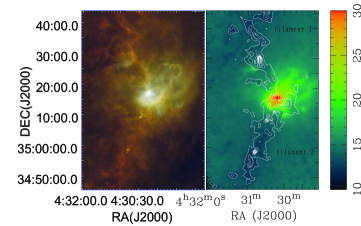
Figure 1: Left panel: three-color image of molecular filament L1482; here, shows red the 250$\mu$m, green the 160$\mu$m, and blue the 70$\mu$m band (Harvey et al. 2013). The shorter wavelengths reveal hot dusts, such as the H ii regions [Sharpless-222; see Sharpless (1959)] around the NGC1579 stellar cluster, which are clearly shown in blue. The longer wavelengths show the cold, dense objects, such as the cold dense filaments plotted in red . Right panel: dust temperature map (36″corresponding to 0.08pc) of filament L1482, with the column density $N_{\rm H_{2}}$ of molecular hydrogen contours overlaid. Contours are plotted from $6.3\times 10^{21}$ to $5.7\times 10^{22}$ cm^-2 with a spacing of $6.3\times 10^{21}$ cm^-2 (10% to 90% of the maximum spaced with 10% contour interval).

3.1 Column density and temperature maps

The column density $N_{\rm H_{2}}$ of molecular hydrogen and dust temperature maps of L1482 filament shown in the right panel of Fig. 1 are derived from Harvey et al. (2013), who fit $160\mu$m, $250\mu$m, $350\mu$m, and $500\mu$m pixel-by-pixel for spectral energy distributions (SEDs) of Könyves et al. (2010) at four longer Herschel wavebands (still with the same 36″spatial resolution) using a simplified model for dust emissions, namely $F_{\nu}=\kappa_{\nu}B(\nu,T)\times$(column density) with the assumed dust opacity law of $\kappa_{\nu}=0.1(\nu/1000{\rm\ GHz})^{\eta}{\rm\ cm}^{2}{\rm\ g}^{-1}$ and a spectral index $\eta=2$. Here, $B(\nu,T)$ is the Planck function defined by $B(\nu,T)=(2h\nu^{3}/c^{2})[\exp(h\nu/kT)-1]^{-1}$, where $T$ denotes the absolute dust temperature, $\nu$ the frequency, $k$ the Boltzmann constant, $h$ the Planck constant, and $c$ the speed of light.

From the column density and temperature maps in the right panel of Fig. 1, we note that the northern and southern parts of L1482 molecular filament are dominated by relatively cold dense gas materials, in contrast to the map center, where warmer dust is heated by the stellar cluster NGC1579.

Table 1: Angular positions and the estimated physical parameters for the 23 identified molecular clumps.

Source	RA	Decl	Peak Column Density	Tdust	Size	Protostar⋆
No. Label	(J2000)	(J2000)	(1022 cm-2)	(K)	[″$\times$″  (°)]	Existence
1	04:31:03.59	+35:42:16.93	1.34	12.1	100 $\times$ 77 ( 52.1 )	no
2	04:30:56.90	+35:39:45.37	1.85	11.5	234 $\times$ 103 (-90.0 )	no
3	04:31:25.08	+35:39:22.76	1.62	12.0	187 $\times$ 150 (-83.2 )	no
4	04:30:47.05	+35:37:27.99	2.18	12.0	251 $\times$ 103 ( 51.4 )	yes
5	04:30:34.51	+35:34:57.04	2.06	11.9	152 $\times$ 86 (-38.4 )	no
6	04:30:40.47	+35:29:25.00	4.52	12.5	253 $\times$ 89 ( 14.6 )	yes
7	04:30:55.74	+35:29:16.76	1.77	12.9	159 $\times$ 97 ( 31.7 )	yes
8	04:30:16.92	+35:23:02.94	1.49	15.9	168 $\times$ 113 ( 13.7 )	no
9	04:30:22.37	+35:19:59.27	1.25	17.7	195 $\times$ 137 ( 56.2 )	no
10	04:30:16.15	+35:17:06.51	1.83	29.7	228 $\times$ 110 (-22.3 )	yes
11	04:29:53.90	+35:15:41.51	2.18	18.9	238 $\times$ 119 ( -5.0 )	yes
12	04:30:02.67	+35:14:15.14	1.89	20.8	195 $\times$ 68 (-63.9 )	yes
13	04:30:14.80	+35:12:07.16	3.50	15.5	172 $\times$ 85 (-19.1 )	no
14	04:30:26.60	+35:10:44.14	1.55	14.2	119 $\times$ 108 (-14.8 )	no
15	04:30:20.06	+35:09:38.44	2.32	13.3	119 $\times$ 83 ( 60.4 )	no
16	04:30:29.88	+35:08:54.14	1.87	13.6	124 $\times$ 100 (-74.6 )	no
17	04:30:13.94	+35:07:46.97	1.80	13.4	103 $\times$ 72 ( 28.8 )	yes
18	04:30:27.83	+35:05:16.42	1.41	13.0	388 $\times$ 201 ( 44.1 )	no
19	04:30:38.95	+35:02:12.12	1.27	12.5	293 $\times$ 189 (-27.9 )	yes
20	04:30:47.54	+34:58:48.27	3.87	12.7	137 $\times$ 68 (-33.6 )	yes
21	04:30:53.98	+34:55:41.59	2.27	11.5	262 $\times$ 93 ( 19.4 )	yes
22	04:30:56.40	+34:54:11.01	2.62	11.1	115 $\times$ 102 (-32.6 )	yes
23	04:31:24.80	+34:50:43.96	1.44	12.1	137 $\times$ 89 ( 63.7 )	no

Table 2: Estimated physical parameters for the 23 identified molecular clumps.

Source	Radius	Mass	n	$\Delta v$	$\sigma_{\mathrm{NT}}$	fturb
No. Label	(pc)	($M_{\odot}$)	(104 cm-3)	(km $s^{-1}$)	(km $s^{-1}$)
1	0.10	6.8	3.8	1.13	0.48	2.5
2	0.17	25.6	2.5	1.08	0.46	2.4
3	0.18	26.7	2.1
4	0.18	32.7	2.9	1.29	0.54	2.9
5	0.12	15.8	3.9	1.44	0.61	3.2
6	0.16	61.3	6.8	1.47	0.62	3.2
7	0.14	16.4	3.2	1.20	0.51	2.6
8	0.15	16.7	2.4	1.36	0.57	2.6
9	0.18	20.2	1.7	0.95	0.40	1.7
10	0.17	25.4	2.4	1.25	0.52	1.7
11	0.18	37.5	2.9	1.65	0.70	2.9
12	0.13	19.8	4.8	1.52	0.64	2.6
13	0.13	18.9	4.0	1.47	0.62	2.9
14	0.12	16.7	4.3	1.65	0.70	3.4
15	0.11	16.2	6.2	1.72	0.73	3.6
16	0.12	15.7	4.2	1.55	0.66	3.2
17	0.09	6.8	4.0	1.52	0.64	3.2
18	0.30	62.8	1.1	1.81	0.77	3.9
19	0.26	43.3	1.2	1.32	0.56	2.9
20	0.11	20.9	8.6	1.36	0.57	2.9
21	0.17	31.1	3.0	1.24	0.52	2.8
22	0.12	19.3	5.7
23	0.12	10.5	2.9

3.2 Molecular line emissions from molecular clouds

The various transitions of carbon monoxide CO spectral lines trace different molecular cloud environments. For example, ¹³CO $J=1-0$ traces somewhat denser regions than ¹²CO $J=1-0$ does. From Fig. 2 (the integrated molecular intensity maps overlaid by the $N_{\rm H_{2}}$ column density contours), we can see that the ¹³CO $J=1-0$ has a similar morphology as that of the dust column density, while ¹²CO $J=2-1$ appears to trace a more extended component. Since the upper energy level temperature and critical number density for ¹²CO $J=3-2$ line transition are 33.2 K and $5\times 10^{4}$ cm^-3, the molecular transition ¹²CO $J=3-2$ traces warmer and denser gas regions (e.g. Kaufman et al. 1999; Qin et al. 2008; Ji et al. 2012). The ¹²CO $J=3-2$ line emission (Fig. 1, right panel) suggests that the molecular gas could be heated by thermal emissions from dusts (e.g. Goldreich & Kwan 1974). The higher resolution velocity field (see Fig. 3 for the first-moment maps) from ¹²CO $J=2-1$ in gray scale is overlaid with the contours of the column densities of hydrogen molecules. All molecular emissions are at the same line-of-sight velocity to within ($-1.5\sim 0.5$) km s^-1, confirming that the filament is a single coherent object, as proposed in Lada et al. (2009) and as first revealed by ¹²CO $J=1-0$ observations.

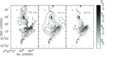
Figure 2: Three molecular line transitions of ¹³CO $J=1-0$, ¹²CO $J=2-1$ and ¹²CO $J=3-2$ shown as integrated molecular intensity maps are overlaid with the column density of hydrogen molecules (H₂). The contours are from 20% to 90% of the peak with an adjacent contour interval of 10%. Molecular emissions integrated from $-3$ km s^-1 to 3 km s^-1 (from the channel maps in Appendix A). The white circle is the location of the stellar cluster NGC1579 and the two straight lines in the left panel indicate the loci for the position-velocity diagrams in Fig. 7.

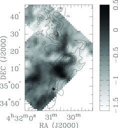
Figure 3: Column density contours (black) are overlaid on the ¹²CO $J=2-1$ intensity-weighted velocity maps (first moment). Contours here are plotted from $6.3\times 10^{21}$ to $5.7\times 10^{22}$ with a spacing of $6.3\times 10^{21}$ (10% to 90% spaced with 10% interval of the maximum). The white circle marks the location of the stellar cluster NGC1579.

3.3 Dense clumps and protostars embedded in filaments

3.3.1 Identifications of molecular clumps along filaments

Based on the column density map, we used a two-step method (e.g. Li et al. 2007) to identify molecular clumps in our acquired data and estimated their physical parameters.

First, we derived the root mean square (rms) of the column density map based on a background noise estimate of $1.7\times 10^{21}$ cm^-2 from weak-emission regions, and then we used the Clumpfind2d algorithm (e.g. Williams et al. 1994) with a threshold of five times the rms noise level to identify the intensity peaks, which must be stronger than seven times the background rms noise level. Using the CLUMPFIND algorithm to locate emission-intensity peaks represents only the first step.

Second, we made a few assumptions about the boundary and shape of these identified molecular clump structures. The boundary was defined as a 5 rms closed contour around the intensity peaks and the shape is a two-dimensional (2D) Gaussian structure. We then used a 2D Gaussian procedure to fit identified molecular clumps within the 5 rms closed boundary around an intensity peak. Finally, we also excluded isolated bright pixel spikes, which tend to appear towards edges of maps. In summary, by using this technique, we identified 23 molecular clumps in the column density map of L1482 molecular filament with their basic properties summarized in Table 1, which includes, for each molecular clump, a numeric identification label, position, peak column density, and dust temperature. In the last column of Table 1, we also indicate whether or not the identified molecular clump contains a protostar as determined previously in the literature (e.g. Gutermuth et al. 2009; Wolk et al. 2010; Harvey et al. 2013). Our simple coincidence criterion is that when the distance between the peak position of a molecular clump and a protostar is smaller than the semi-minor axis of the clump ellipse, the molecular clump is regarded as containing a protostar. Positions of molecular clumps and known protostars are marked on both the column density and dust temperature maps in Fig. 4.

The peak column densities of these molecular clumps fall in the range of [$1.25-4.52]\times 10^{22}$ cm^-2, with an average value of $2.08\pm 0.84\times 10^{22}$ cm^-2. The peak dust temperature of these molecular clumps ranges from 11.1 to 29.7 K, with an average value of $14.4\pm 4.2$ K.

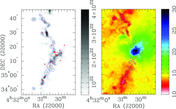
Figure 4: Left panel: column density with dust clumps. The red asterisk symbols represent protostars as determined by Gutermuth et al. (2009), Wolk et al. (2010) and Harvey et al. (2013). Right panel: dust temperatures overlaid with molecular hydrogen clumps marked by blue ellipses (in both panels).

3.3.2 Parameter estimates for the identified clumps

The masses of these identified molecular clumps are estimated by $M=\beta\ m_{\rm H_{2}}N_{\rm total,H_{2}}(D\Delta)^{2}$ (e.g. Lee et al. 2012; Qian et al. 2012; Lee et al. 2013), where $\beta=1.39$ converts the hydrogen mass into total mass taking into account the helium abundance (e.g. Williams et al. 1994), $m_{\rm H_{2}}$ is the mass of a hydrogen molecule, ${N_{\rm total,H_{2}}}$ is the total estimated clump column density of H₂, $D\sim 450$ pc is the distance to the CMC, and $\Delta=14\arcsec$ is the pixel angular size of the data (e.g. Harvey et al. 2013). The estimated molecular clump masses are shown in column 3 of Table 2. The molecular clump masses range from 6.8 to $62.8M_{\odot}$, with an average value of $24.7_{-16.2}^{+31.1}M_{\odot}$. The average mass of molecular clumps containing protostars is $28.6M_{\odot}$, while the average mass of the starless clumps is $21.0M_{\odot}$. Thus, there might be a slightly increased average mass in the case of molecular clumps with embedded protostars than in that of starless molecular clumps, although it may not represent a significant systematic difference. The radii of the identified molecular clumps are defined by $R=\sqrt{ab}/2$, where $a$ and $b$ are the major and minor axes of a clump ellipse. The estimated clump radii are listed in column 2 of Table 2 and range from 0.10 to 0.30 pc, with an average value of $0.15\pm 0.05$ pc. The volume number densities for molecular hydrogen H₂ of these clumps are inferred according to the expression $n=3M/(4\pi R^{3}m_{\rm H_{2}})$. The estimated volume number densities are shown in column 4 of Table 2, they range from 1.1 to $8.6\times 10^{4}$ cm^-3, with an average value of $3.7\pm 1.8\times 10^{4}$ cm^-3. The average radius $\sim 0.15$ pc of the identified molecular clumps in our data analysis is comparable to that of the identified CS clumps in the molecular cloud Orion A, $\sim 0.16$ pc, and that of the identified NH₃ clumps in the molecular cloud Perseus, $\sim 0.12$ pc. But mean mass of the identified molecular clumps of our data analysis is considerably smaller than that of the CS clumps in the molecular cloud Orion A, $>100M_{\odot}$ (e.g., Tatematsu et al. 1993), and is systematically larger than that of the NH₃ clumps in the molecular cloud Perseus, $\sim 9M_{\odot}$ (e.g., Ladd et al. 1994).

Kauffmann & Pillai (2010) gave an empirical mass-radius threshold for massive star formation, namely $M(r)=870M_{\odot}(r/\rm pc)^{1.33}$, above which massive stars form. We invoke this criterion to examine our identified molecular clumps $-$ their masses as a function of radius are shown in Fig. 6. Based on this empirical mass-radius threshold, our identified molecular clumps may not form massive stars. Li et al. (2013a) found $\sim 40$% of the molecular clumps in the Orion nebula above this threshold. While strikingly similar in mass and size to the better known Orion molecular cloud (OMC), the formation rate for high-mass stars appears to be more depressed in the CMC than that in the OMC.

4 Analysis and discussion

4.1 Gravitational instabilities for dense molecular clumps

4.1.1 Velocity dispersion and turbulence

We used the molecular transition ¹³CO $J=1-0$ linewidths to calculate the nonthermal contribution of the line-of-sight velocity dispersion (averaged over one 1′ beam size) and the level of internal flow turbulence. The nonthermal ($\sigma_{\mathrm{NT}}$) and thermal ($\sigma_{\mathrm{Therm}}$) one-dimensional velocity dispersions in our identified molecular clumps were calculated according to the formulae of Myers (1983):

$$\sigma_{\mathrm{NT}}=\bigg{(}\sigma_{{}^{13}\rm CO}^{2}-\frac{kT_{\rm kin}}{m_{{}^{13}\rm CO}}\bigg{)}^{1/2}\,,$$ (1)

$$\sigma_{\mathrm{Therm}}=\bigg{(}\frac{kT_{\rm kin}}{m_{\rm H}\mu}\bigg{)}^{1/2}\,,$$ (2)

where $\sigma_{{}^{13}\rm CO}$ is the one-dimensional velocity dispersion of ¹³CO$(1-0)$ related to the FWHM linewidth ($0.95\sim 1.81$ km s^-1 with an average of $1.40\pm 0.22$ km s^-1; see column 5 of Table 2) as $\sigma=\Delta v/2.355$. Here, the dust temperature is taken as T_kin with $k$ being the Boltzmann constant, $m_{{}^{13}\rm CO}$ is the mass of a ¹³CO molecule, $m_{\rm H}$ is the mass of an atomic hydrogen, and $\mu=2.72$ is the mean molecular weight of a molecular hydrogen ISM gas. Furthermore, the level of internal flow turbulence is given by the ratio $f_{\mathrm{turb}}=\sigma_{\mathrm{NT}}/\sigma_{\mathrm{Therm}}$, where $\sigma_{\mathrm{Therm}}$ is the one-dimensional isothermal sound speed in a molecular hydrogen ISM cloud. The $f_{\mathrm{turb}}=\sigma_{\mathrm{NT}}/\sigma_{\mathrm{Therm}}$ ratios versus the molecular clump masses are shown in Fig. 5 and all molecular clumps appear to be supersonic. The values of $\sigma_{\mathrm{NT}}$ and $f_{\mathrm{turb}}$ are given in columns 6 and 7 in Table 2. The $\sigma_{\mathrm{NT}}$ ranges from 0.40 to 0.77 km s^-1 with an average value of $0.59\pm 0.10$ km s^-1. The $f_{\mathrm{turb}}$ ranges from 1.7 to 3.9 with an average value of $2.9\pm 0.5$.

Figure 5: $f_{\mathrm{turb}}=\sigma_{\mathrm{NT}}/\sigma_{\mathrm{Therm}}$ ratios versus molecular clump masses in units of the solar mass $M_{\odot}$. The horizontal dashed line for $\sigma_{\mathrm{NT}}/\sigma_{\mathrm{Therm}}=1$ is the demarcation between subsonic and supersonic nonthermal motions.

4.1.2 Static Bonnor-Ebert sphere model

To examine the dynamic state of molecular clumps, we assumed that these clumps are only thermally supported against the gas self-gravity.

Figure 6: Mass (in units of solar mass $M_{\odot}$) versus radius (in units of pc) of the molecular clumps in our sample compared with the static Bonnor-Ebert sphere. The top curve [e.g. Kauffmann & Pilltai (2010)] represents the mass-radius threshold for forming massive stars. The other curves are the critical masses that can be supported for clumps of specified temperatures and sizes. T${}_{\mathrm{eq}}=51$ K corresponds to a turbulent linewidth of $\sim 1$ km s^-1 (FWHM), and 165 K corresponds to a linewidth of $\sim 1.8$ km s^-1.

We computed the static Bonnor-Ebert mass-radius relation for a spherical, self-gravitating, isothermal, and hydrostatic molecular clump. The Bonnor-Ebert mass is obtained by integrating the mass density profile of the Bonnor-Ebert sphere, with an approximate analytic expression invoked by Tafalla et al. (2004) as follows:

$$\rho(\xi)=1/[1+(\xi/2.25)^{2.5}]\ \,,$$ (3)

$$\xi=r(4\pi G\rho_{c}/v_{s}^{2})^{1/2}\ \,,$$ (4)

where $\rho_{c}$ is the central mass density and $v_{s}=[kT/(\mu m_{H})]^{1/2}$ is the isothermal sound speed. Ebert (1955) and Bonnor (1956) pointed out that when the dimensionless radial variable $\xi$ exceeds a critical value of 6.5, there is no longer any stable Bonnor-Ebert sphere solution. Assuming $\xi_{max}=6.5$ and using the observed clump radius, the central mass density $\rho_{c}$ can be determined and then the critical clump mass $M_{\rm BE-CR}$ can be readily calculated by integrating equations (3) and (4).

In Fig. 6, the sizes and masses of molecular clumps are plotted along with the calculated curves based on critical static Bonnor-Ebert (BE) spheres at various gas temperatures. Our identified molecular clumps appear to be too massive to be stable BE spheres for a kinetic temperature as high as $\sim 20$ K. One important caveat for this analysis and discussion is that the observed size of our molecular clumps are not as clearly defined as required by the theoretical model. Nevertheless, the considerable excesses of the observed molecular clump mass relative to the BE critical mass do suggest that increasing the clump size by as much as a factor of a few would not make a clump thermally stable against the self-gravity. The important significance of our data analysis is that our identified molecular clumps here are not expected to be in static equilibria. These molecular dense clumps are most likely in dynamic processes of being formed on the spot (Lou & Shen 2004; Shen & Lou 2004, 2006). It seems apparent that dynamic evolutions of these star-forming and/or dense starless molecular clumps are inevitable (Lou & Gao 2006; Gao et al. 2009; Gao & Lou 2010). For quasi-spherical molecular clumps in hydrodynamic evolution, it is possible to use at least four major observational diagnostics to constrain self-consistent dynamic models coupled with radiative transfer calculations (e.g. Lou & Gao 2011; Fu et al. 2011), namely, extensive observations of various properties of molecular lines (e.g. line profiles), submillimeter continuum emissions from thermal dusts, and dust extinction observations as well as neutral hydrogen 21cm absorption lines in MCs.

To evaluate the importance of gas flow turbulence in molecular clumps, we also considered a modified BE sphere model taking into account turbulence in an empirical manner (Lai et al. 2003). We can define an equivalent temperature as

$$T_{\mathrm{eq}}=\frac{m_{\mathrm{H}}\Delta V^{2}}{8\ln(2)k}\,,$$ (5)

where $\Delta V$ is the total FWHM linewidth of the gas. The observed FWHM linewidth of ¹³CO $J=1-0$ at $1\arcmin$ scale towards these regions ranges from 1.0 to 1.8 km s^-1. We have plotted the critical mass curves based on $T_{\rm eq}$ ($\Delta V=1$ km s^-1 ) and $T_{\rm eq}$ ($\Delta V=1.8$km s^-1) in Fig. 6. Assuming a FWHM linewidth of 1 km s^-1, most of molecular clumps appear to be supercritical. This is in contrast to molecular clumps identified in the Taurus molecular cloud, where most molecular clumps remain subcritical (e.g. Qian et al. 2012).

4.2 Fragmentation along a molecular filament

4.2.1 Formation of molecular clumps

The formation of molecular clumps may proceed in two main stages based on Herschel observational results (e.g. André et al. 2010, 2011). First, large-scale magnetohydrodynamic (MHD) turbulence generates a complex network of molecular filaments in the interstellar medium (ISM) (e.g. Padoan et al. 2001; Balsara et al. 2001). In the second stage, the self-gravity takes over and fragments the densest molecular filaments into prestellar clumps via gravitational collapse instabilities (e.g. Inutsuka & Miyama 1997; Ostriker 1964).

The critical mass per unit length, $M_{line}^{crit}=2c_{s}^{2}/G$ (where $c_{s}$ is the isothermal sound speed and $G$ is the gravitational constant) is the critical value required for a molecular filament to be gravitationally unstable to radial contraction and fragmentation along its length (e.g. Inutsuka & Miyama 1997). Remarkably, this critical line mass only depends on the gas temperature (Ostriker 1964). It is approximately equal to $\sim$ 16 M_⊙/pc for molecular gas filaments at T$=10$ K, corresponding to a $c_{s}\sim 0.2$ km s^-1. Arzoumanian et al. (2013) assumed that ISM filaments have Gaussian radial column density profiles, an estimate of the mass per unit lengh is given by M_line $\approx\Sigma_{0}\times W_{fil}$, where $W_{fil}$ is the typical filament width (André et al. 2010; Arzoumanian et al. 2013) and $\Sigma_{0}=\mu\ m_{\rm H}N_{\rm H_{2}^{0}}$ is the central gas surface mass density of a filament. For a typical filament width of $\sim$ 0.1 pc, the theoretical value of $\sim$ 16 M_⊙/pc corresponds to a central column density $N_{\rm H_{2}}^{0}\sim 8\times 10^{21}$ cm^-2. These filaments may be grouped into thermally supercritical and thermally subcritical filaments depending on whether their line masses higher or lower than 16 M_⊙/pc correspond to a central column density $N_{\rm H_{2}}^{0}\sim 8\times 10^{21}$ cm^-2. Thermally supercritical filaments are expected to be globally unstable to radial gravitational collapse and fragmentation into prestellar clumps along their lengths. The prestellar clumps formed in this manner are themselves expected to collapse locally into protostars in dense molecular clumps.

Since the central number density of molecular filament 1 ( the average value of peak density for all clumps located within molecular filament 1) is $\sim 2.0\times 10^{22}$ cm^-2 and that of molecular filament 2 ( the average value of the peak density for all clumps located within molecular filament 2) is $\sim 2.3\times 10^{22}$ cm^-2 (both above $8\times 10^{21}$ cm^-2), they all appear to be thermally supercritical filaments. Therefore, the L1482 filamentary cloud appears to be a thermally supercritical structure, susceptible to gravitational fragmentation. Li et al. (2013b) studied magnetic fields of filamentary clouds in the Gould Belt and found that the density threshold of cloud gravitational contraction is $\sim 10^{22}$ cm^-2. Still, these molecular filaments remain susceptible to gravitational fragmentation, in qualitative agreement with the detected clumps and protostars. This last stage of filament-to-clumps evolution seems to emerge as a phenomenon often found in recent observational studies.

We have already indicated in the earlier discussion that MHD turbulence is likely to play a major role in creating the filamentary network in the magnetized ISM according to observations and numerical simulations. For an individual magnetized filament with a mean magnetic field $B_{0}$ along the filament, the Jeans length for gravitational collapse instability transverse to the filament $\lambda_{\perp}=[\pi(C_{S}^{2}+C_{A}^{2})/(\rho_{0}G)]^{1/2}$ becomes larger (Chandrasekhar & Fermi 1953; Lou 1996), where $C_{S}$ is the sound speed and $C_{A}=B_{0}/(4\pi\rho_{0})^{1/2}$ is the Alfvén wave speed. Although the Jeans length for gravitational collapse instability along the filament remains the same as the hydrodynamic one, the growth rates of these instabilities change and become anisotropic due to the very presence of the mean magnetic field $B_{0}$. For a large-amplitude circularly polarized incompressible Alfvén wave train propagating along such a mean magnetic field aligned with an ISM filament, the Jeans lengths for gravitational collapse instabilities are increased in all directions anisotropically because a large-amplitude Alfvén wave train involves a transverse magnetic field relative to the mean $B_{0}$ direction. Therefore, such magnetized collapsed clumps should have systematically larger masses, depending on the magnetic field strengths (Lou 1996). For a magnetized ISM with MHD turbulence, both turbulent flow velocities and random magnetic fields tend to increase the volume and mass of a collapsed molecular clump in general (e.g. Strittmatter 1966; Rees 1987). It is therefore of considerable interest to measure magnetic field strengths and turbulent flow velocities in such ISM filamentary network and dense molecular clumps embedded in individual filaments. Without any polarimetric observations available at the moment, the presence of a strong, permeating magnetic field in MCs and molecular filaments remains still hypothetical.

Empirically, magnetic field strengths in the ISM may range from a few $\mu$G to several hundred $\mu$G. By the common wisdom of equipartition in energies, we tend to suggest that the sound speed $C_{S}$ and the Alfvén speed $C_{A}$ may be comparable. Along this line of arguments for an ISM with random magnetic fields, the Jeans volume for a collapsing molecular clump may be $\sim$ three times larger than that in the absence of magnetic field. By these estimates, the molecular clumps studied here remain supercritical even when an equipartition random magnetic field is taken into account.

4.2.2 Role of turbulence in molecular clumps

The ¹³CO $J=1-0$ line emission probes nonthermal supersonic linewidths, implying that the internal flow structures of a $\sim$ MC, molecular clumps and their environments may be highly turbulent. As such, (MHD) turbulence would play an important role in the process of dynamic fragmentation. It might be the case that CO isotopes are tracing a low-density, more turbulent component of the gas, that these clumps are most likely substructured as indicated by turbulent fragmentation models, and that with higher resolution, a different dense gas tracer is required to resolve individual cores of smaller scales with more coherent gas motions. In particular, interferometric observations with a tracer [e.g. CS(2-1)] of higher resolution are necessary to demonstrate that further fragmentation within each clump (broken into groups of $4-5$ pieces) may occur at the prestellar stage, as in the case of the OMC (e.g. Lee et al. 2013). Approximately along the central axes of molecular filaments 1 and 2 as shown in Fig. 2, we made their position-velocity diagrams in Fig. 7. Filament 1 clearly shows velocity gradients. These gradients might be related to inflows along the filament (e.g. Lee et al. 2013). For example, molecular filament 1 might involve supersonic converging flows along the filament to feed embedded molecular clumps containing protostars and/or cluster of subcomponents.

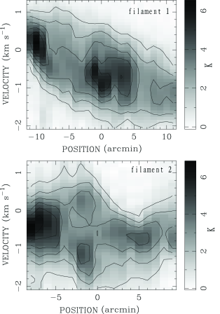
Figure 7: Position-velocity diagrams of the ¹³CO $J=1-0$ emission along the two marked straight lines in the left panel of Fig. 2. The contour levels in both panels are 10% to 60% of the peak value spaced with 10% contour interval, successively.

5 Conclusion and summary

We have conducted a comparative and comprehensive mapping study for molecular transition lines of ¹³CO $J=1-0$ (Delingha), ¹²CO $J=2-1$ and ¹²CO $J=3-2$ (KOSMA) and multiband infrared data of Herschel spacecraft observations towards the molecular filament L1482 in CMC. The main results of our data analysis and parameter estimates are summarized below.

(1) The L1482 molecular filament is most likely a spatially coherent global structure, as shown by the more or less uniform ¹²CO $J=2-1$ line-of-sight velocities throughout the MC.

(2) As the NGC1579 stellar cluster is physically located at the junction of the two main molecular filaments 1 and 2, we propose that NGC1579 stellar cluster might originate from molecular filament merger processes involving converging inflows to feed the cluster and molecular clumps.

(3) We have identified 23 molecular clumps in this region. The peak column densities of these molecular clumps range from 1.25 to $4.52\times 10^{22}$ cm^-2, with an average value of $2.08\pm 0.84\times 10^{22}$ cm^-2. The peak dust temperature of these molecular clumps ranges from 11.1 to 29.7 K, with an average value of $14.4\pm 4.2$ K. The radii of these molecular clumps range from 0.10 to 0.30 pc, with an average value of $0.15\pm 0.05$ pc. The number densities range from 1.1 to $8.6\times 10^{4}$ cm^-3, with an average value of $3.7\pm 1.8\times 10^{4}$ cm^-3. The masses range from 6.8 to 62.8$M_{\odot}$, with an average value of $24.7_{-16.2}^{+31.1}M_{\odot}$. Eleven molecular clumps are found to be associated with protostars, and the star-formation processes are most likely ongoing. If follows that the defined protostellar and starless subsamples of molecular clumps have similar temperatures and linewidths, but perhaps different masses, with an average mass of $28.6M_{\odot}$ for the former, which is slightly more massive than $21.0M_{\odot}$ than the latter; it would be of considerable interests to further confirm whether this is indeed a systematic difference, because resolving substructures of molecular clumps is impossible with the currently available data. The average radius of the identified molecular clumps in our data analysis, $\sim 0.15$ pc, is comparable to that of the identified CS clumps in the molecular cloud Orion A, $\sim 0.16$ pc, and that of the identified NH₃ clumps in the molecular cloud Perseus, $\sim 0.12$ pc. However, the mean mass of the identified molecular clumps in our data analysis is considerably smaller than that of the identified CS clumps in the molecular cloud Orion A, $>100M_{\odot}$, and is systematically larger than that of the identified NH₃ clumps in the molecular cloud Perseus, $\sim 9M_{\odot}$.

(4) The $\sigma_{\rm NT}$ of these molecular clumps ranges from 0.40 to 0.77 km s^-1, with an average value of $0.59\pm 0.10$ km s^-1. The ratio $f_{\rm turb}$ of these molecular clumps ranges from 1.7 to 3.9, with an average value of $2.9\pm 0.5$. Our identified molecular clumps typically show supersonic nonthermal motions according to the estimates.

(5) Based on the empirical mass-radius threshold of a static Bonnor-Ebert sphere model with effects of turbulence empirically included via an effective temperature (e.g. Lai et al. 2003), our identified molecular clumps may not be able to form massive stars. While surprisingly similar in mass and size to the well-known Orion molecular cloud, the rate of forming high-mass stars is considerably lower in the CMC than that in the OMC.

(6) Our critical mass per unit length estimates suggest that molecular filaments examined here are thermally supercritical and molecular clumps most likely involve dynamic processes of gravitational fragmentation along the molecular filaments.

(7) By the equipartition argument for energies, the presence of mean as well as random magnetic fields tends to increase the Jeans mass of a collapsing mass. The masses of our identified molecular clumps appear to be still supercritical even in the presence of such equipartition magnetic fields. This seems to suggest that instead of being static, these molecular clumps are most likely in the stage of hydrodynamic or MHD evolution.

(8) Molecular filament 1 shows clear velocity gradients. These gradients might be partly associated with inflows along filaments. Such flows may play important roles of feeding stellar cluster and molecular clumps during star formation processes along molecular filament L1482.

Appendix A ¹²CO $J=2-1$ and ¹²CO $J=3-2$ channel maps as derived from our KOSMA observations in the Swiss Alps.

Figs. 8 and 9 present channel maps for the two molecular line transitions ¹²CO $J=2-1$ and ¹²CO $J=3-2$ integrated over narrow ranges in $V_{\rm LSR}$. The molecular line data were acquired by the KOSMA 3-m telescope in the Swiss Alps. Detailed descriptions of the observations can be found in Section 2.

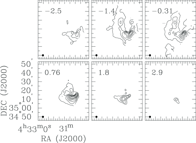
Figure 8: Molecular transition ¹²CO $J=2-1$ channel maps. The center velocities are shown in the upper left corners of each panel in units of km s^-1. The integrated velocity interval in each panel is 1.1 km s^-1. The contour levels are from 20% up to 90% of the peak with an adjacent contour intervals of 10%. The black solid circle in the lower left corner gives the beam size.

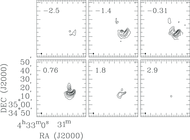
Figure 9: Molecular ¹²CO $J=3-2$ channel maps. The center velocities are shown in the upper left corners of each panel in units of km s^-1. The integrated velocity interval in each panel is 1.1 km s^-1. The contour levels are from 20% up to 90% of the peak with an adjacent 10% contour interval. The black solid circle in the lower left corner gives the beam size.