Incorporating Sharp Features in the General Solid Sweep Framework

Abstract

This paper extends a recently proposed robust computational framework for constructing the boundary representation (brep) of the volume swept by a given smooth solid moving along a one parameter family $h$ of rigid motions. Our extension allows the input solid to have sharp features, i.e., to be of class G0 wherein, the unit outward normal to the solid may be discontinuous. In the earlier framework, the solid to be swept was restricted to be G1, and thus this is a significant and useful extension of that work.

This naturally requires a precise description of the geometry of the surface generated by the sweep of a sharp edge supported by two intersecting smooth faces. We uncover the geometry along with the related issues like parametrization, self-intersection and singularities via a novel mathematical analysis. Correct trimming of such a surface is achieved by a delicate analysis of the interplay between the cone of normals at a sharp point and its trajectory under $h$. The overall topology is explicated by a key lifting theorem which allows us to compute the adjacency relations amongst entities in the swept volume by relating them to corresponding adjacencies in the input solid. Moreover, global issues related to body-check such as orientation are efficiently resolved. Many examples from a pilot implementation illustrate the efficiency and effectiveness of our framework.

1 Introduction

In this paper we investigate the computation of the volume swept by a given solid moving along a smooth one parameter family of rigid motions. We assume the solid to be of class G0, wherein, the unit outward normal may be discontinuous at the intersection of two or more faces. Solid sweep has several applications, viz. CNC-machining verification [16, 17], collision detection, motion planning [1] and packaging [20]. An example of solid sweep appears in Fig. 1. We adopt the industry standard parametric boundary representation (brep) format to input the solid and output the swept volume. In the brep format, the solid $M$ is represented by its boundary $\partial M$ which separates the interior of $M$ from its exterior. The brep of $M$ consists of the parametric definitions of the faces, edges and vertices as well as their orientations and adjacency relations amongst these. Fig. 2 schematically illustrates such a solid.

Figure 1: An example of swept volume.

The computation of swept volume has been extensively studied [2, 6, 8, 9, 10, 11, 13, 14]. In [2], the envelope ${\cal E}$ is modeled as the the set of points where the Jacobian of the sweep map is rank deficient. The authors rely on symbolic computation hence this method cannot accept free form surfaces such as splines as input. In [6], the authors derive a differential equation whose solution is the envelope ${\cal E}$ of the swept volume ${\cal V}$. A set of points on ${\cal E}$ is sampled through which a surface is fitted to obtain an approximation of ${\cal E}$. This method accepts smooth solids as input. Further it may not meet the tolerance requirements of modern geometry kernels. In [9], the authors give a complete characterization of the points which are inside, outside or on the boundary of the swept volume by giving a point membership test (PMC). This approach handles class G0 solids, effectively giving a procedural implicit definition (as a PMC) of the swept volume. Conversion from this format to, say, brep format is computationally expensive. In [16], the authors compute the volume swept by a class G0 cutting tool undergoing 5-axis motion by employing the T-map, i.e., the outward normals to the tool at a point. This method is limited to sweeping tools which are bodies of rotation, and hence, have radial symmetry. It does not generalize to sweeping free form solids. In [18], the authors present an error-bounded approximation of the envelope of the volume swept by a polyhedron along a parametric trajectory. They employ a volumetric approach using an adaptive grid to provide a guarantee about the correctness of the topology of the swept volume. This approach, however, may not meet the tolerance requirements of CAD kernels while being computationally efficient at the same time. In [12], the authors approximate the given trajectory by a continuous, piecewise screw motion and generate candidate faces of the swept surface. In order to performing trimming, the inverse trajectory method is used. Limitations of this method are clear, viz, restriction on the class of motions along which the sweep occurs.

In [5], the authors present the first complete computational framework for constructing the brep of ${\cal V}$ which is derived from the brep of $M$. Local issues like adjacency relations amongst geometric entities of ${\cal E}$ as well as global issues such as their orientation are analysed assuming that $M$ is of class G1. Key constructs such as the prism and the funnel are used to parametrize the faces of ${\cal V}$ and guide the computation of orientation of co-edges bounding faces of ${\cal V}$.

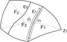
Figure 2: Brep of a solid.

In this paper we extend the framework proposed in [5] to input solids of class G0. This, along with the topology and geometry generated by smooth faces of $\partial M$ explicated in [5] and the trimming of swept volume described in [4] gives a complete framework for computing the brep of the general swept volume.

An edge or a vertex of $\partial M$ is called sharp if it lies in the intersection of faces meeting with G1-discontinuity. For instance, in the solid shown in Fig. 2, the faces $F_{1}$ and $F_{2}$ meet in the sharp edge $E_{1}$ while faces $F_{2}$ and $F_{3}$ meet smoothly in edge $E_{2}$. The partner co-edges $c_{1}$ and $c_{1}^{\prime}$ for $E_{1}$ associated with faces $F_{1}$ and $F_{2}$ respectively and a sharp vertex $Z_{1}$ are also shown. While modeling mechanical parts, sharp corners and edges are inevitable features. Thus this is an important extension of the aforesaid framework.

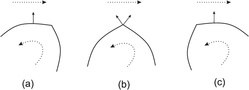
Figure 3: Geometry generated by sharp features.

In this work we focus on the entities in the brep of ${\cal E}$ which are generated by sharp edges and vertices of $\partial M$. This involves the following considerations.

1. Geometry: The local geometry of the entity ${\cal E}^{E}$ in the brep of ${\cal E}$ generated by a sharp edge $E\subset\partial M$ can be modeled by that of the ’free’ edge $E$ moving in $\mathbb{R}^{3}$. The surface $S^{E}$ swept by such an edge is smooth except when the velocity at a point is tangent to the edge at that point.

2. Trim: In order to obtain ${\cal E}^{E}$, $S^{E}$ needs to be suitably trimmed. The correct trimming follows as a result of the interplay between the cone of normals at a sharp point and the trajectory of the point under the family of rigid motions. In the schematic shown in Fig. 3, an object with sharp features undergoes translation with compounded rotation indicated with dotted arrows. In the positions shown in Fig. 3(a) and Fig. 3(c), the sharp feature does not generate any points on the envelope while in Fig. 3(b) it does.

3. Orientation: The faces ${\cal E}^{E}$ must be oriented so that the unit normal at each point of ${\cal E}^{E}$ points in the exterior of the swept volume ${\cal V}$.

We now outline the structure of this paper. In Section 2, we establish a natural correspondence $\pi$ between the boundary of the input solid and the boundary of the swept volume. This serves as a basis for a brep structure on ${\cal E}$. In Section 3 we give the overall solid sweep framework and outline how it extends the framework proposed in [5] to handle sharp features of $\partial M$. In Section 4 we elaborate on the interaction of the unit cone of normals and the trajectory. In Section 5 we parametrize the faces and edges of ${\cal E}$ generated by sharp features of $\partial M$. In Section 6 we analyse the adjacency relations amongst of entities of ${\cal E}$ via the correspondence map $\pi$. We show that there is local similarity between the brep structure of ${\cal E}$ and that of $\partial M$. In Section 7 we explain the steps of the overall computational framework given in Section 3. We give many sweep examples demonstrating the effectiveness of our algorithm. In Section 8, we discuss subtle issues of self-intersections and how they can be handled. Finally, we conclude in Section 9 with remarks on extension of this work.

2 Mathematical structure of the sweep

In this section we define the envelope obtained by sweeping the input solid $M$ along the given trajectory $h$.

Definition 1

A trajectory in $\mathbb{R}^{3}$ is specified by a map

$$h:I\rightarrow(SO(3),\mathbb{R}^{3}),h(t)=(A(t),b(t))$$

where $I$ is a closed interval of $\mathbb{R}$, $A(t)\in SO(3),b(t)\in\mathbb{R}^{3}$. The parameter $t$ represents time.

We assume that $h$ is of class $C^{k}$ for some $k\geq 2$, i.e., partial derivatives of order up to $k$ exist and are continuous.

We make the following key assumption about $(M,h)$.

Assumption 2

The tuple $(M,h)$ is in a general position.

Definition 3

The action of $h$ (at time $t$ in $I$) on $M$ is given by $M(t)=\{A(t)\cdot x+b(t)|x\in M\}$. The swept volume ${\cal V}$ is the union $\bigcup_{t\in I}M(t)$ and the envelope ${\cal E}$ is defined as the boundary of the swept volume ${\cal V}$.

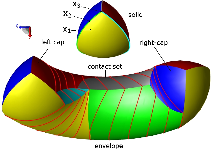
Figure 4: A solid undergoing translation along a circular arc in $xy$-plane and rotation about $y$-axis. Curves of contact at few time instants are shown on the envelope in red.

An example of a swept volume appears in Fig. 4. Clearly, for each point $y$ of ${\cal E}$ there must be an $x\in M$ and a $t\in I$ such that $y=A(t)\cdot x+b(t)$.

We denote the interior of a set $W$ by $W^{o}$ and its boundary by $\partial W$. It is clear that ${\cal V}^{o}=\cup_{t\in I}M(t)^{o}$. Therefore, if $x\in M^{o}$, then for all $t\in I$, $A(t)\cdot x+b(t)\notin{\cal E}$. Thus, the points in the interior of $M$ do not contribute any point on the envelope.

Definition 4

For a point $x\in M$, define the trajectory of $\boldsymbol{x}$ as the map $\gamma_{x}:I\to\mathbb{R}^{3}$ given by $\gamma_{x}(t)=A(t)\cdot x+b(t)$ and the velocity $v_{x}(t)$ as $v_{x}(t)=\gamma_{x}^{\prime}(t)=A^{\prime}(t)\cdot x+b^{\prime}(t)$.

Now we recall the fundamental proposition ([6, 5]) which assumes that $M$ is smooth and provides a necessary condition for a point $x\in\partial M$ to contribute the point $\gamma_{x}(t)$ on ${\cal E}$ at time $t$.

Proposition 5

Let $M$ be smooth and for $x\in\partial M$, let $N_{x}$ be the unit outward normal to $M$ at $x$. Define the function $G:{\partial M}\times I\rightarrow\mathbb{R}$ as $G(x,t)=\left<A(t)\cdot N_{x},v_{x}(t)\right>$. In other words, $G(x,t)$ is the dot product of the velocity vector with the unit outward normal at the point $\gamma_{x}(t)\in\partial M(t)$.

Further, let $I=[t_{0},t_{1}],t\in I$ and $x\in\partial M$ be such that $\gamma_{x}(t)\in\mathcal{E}$. Then either (i) $G(x,t)=0$ or (ii) $t=t_{0}$ and $G(x,t)\leq 0$, or (iii) $t=t_{1}$ and $G(x,t)\geq 0$.

Now we develop some notation in order to generalize the above proposition to non-smooth $M$ represented in the brep format. Recall that the brep of $M$ models $\partial M$ through a collection of faces which meet each other across edges which in turn meet at vertices. Clearly, the sharp features of $M$ are located along the edges and vertices.

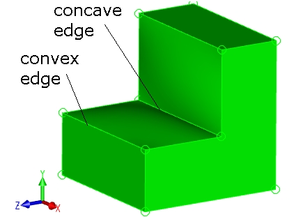
Figure 5: Convex and concave edges on a solid.

The solid $M$ may be (partly) convex/concave at a sharp edge. See Fig. 5 for an example. For the moment we only consider solids that do not have concave edges. See Section 8 for a discussion on concave edges. Further, for simplicity, we assume that at most three faces meet at a sharp vertex in $\partial M$.

Definition 6

For a point $x\in\bigcap_{i=1}^{m}F_{i}$, define the cone of unit (outward) normals (to $\partial M$) at $x$ as the intersection of the unit sphere $S^{2}$ with the cone formed by $N_{i}$, for $i=1,\ldots,m$, where $N_{i}$ is the unit outward normal to $F_{i}$ at $x$. For simplicity, we assume that $N_{i}$ for $i=1,\ldots,m$ are linearly independent. We denote the cone of unit normals at $x$ by $N_{x}$.

The points labeled $x_{3}$ and $x_{2}$ in Fig. 4 lie in the intersection of three and two smooth faces respectively meeting sharply. The point labeled $x_{1}$ lies in the interior of a smooth face, hence $N_{x_{1}}$ has a single element, namely, outward normal to $\partial M$ at $x_{1}$. The cone of normals is referred to as the extended Tool map in [16].

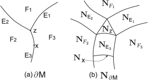
Figure 6: A solid and its unit normal bundle.

Definition 7

For a subset $X$ of $\partial M$, the unit normal bundle (associated to $X$) is defined as the disjoint union of the cones of unit normals at each point in $X$ and denoted by ${\bf N_{X}}$, i.e., ${\bf N_{X}}=\bigsqcup_{x\in X}{N}_{x}=\bigcup_{x\in X}\{(x,n)|n\in{N}_{x}\}$.

In Fig. 6(a) a portion of $\partial M$ is shown in which three faces $F_{i}$ and three edges $E_{i}$ meet at a sharp vertex $Z$. Note that for $X\subset\partial M$, ${\bf N_{X}}\subset\mathbb{R}^{3}\times S^{2}$, where $S^{2}$ is the unit sphere in $\mathbb{R}^{3}$. However, for the ease of illustration we have shown the unit normal bundles ${\bf N_{F_{i}}},{\bf N_{E_{i}}}$ for $i=1,2,3$ and ${\bf N_{Z}}$ schematically in Fig. 6(b) in which an element $(x,n)\in{\bf N_{\partial M}}$ is represented as the ‘offset’ point $x+n$.

For $x\in\partial M$ and $t\in I$, the cone of unit normals to $\partial M(t)$ at the point $\gamma_{x}(t)$ is given by $A(t)\cdot{N}_{x}:=\{A(t)\cdot n|n\in{N}_{x}\}$. Further, the action of $h$ at time $t\in I$ on the unit normal bundle ${\bf N_{\partial M}}$ is given by ${\bf N_{\partial M}}(t):=\{(\gamma_{x}(t),A(t)\cdot n)|x\in\partial M,n\in{N}_{x}\}$.

Definition 8

For $(x,n)\in{\bf N_{\partial M}}$ and $t\in I$, define the function $g:{\bf N_{\partial M}}\times I\to\mathbb{R}$ as $g(x,n,t)=\left<A(t)\cdot n,v_{x}(t)\right>$.

Thus, $g(x,n,t)$ is the dot product of the velocity with the normal $A(t)\cdot n\in A(t)\cdot{N}_{x}$ at the point $\gamma_{x}(t)\in\partial M(t)$.

We are now ready to state the next Proposition which is a natural generalization of Proposition 5 to non-smooth solids.

Proposition 9

Let $I=[t_{0},t_{1}],t\in I$ and $x\in\partial M$ be such that $\gamma_{x}(t)\in\mathcal{E}$. Then either (i) $t=t_{0}$ and there exists $n\in{N}_{x}$ such that $g(x,n,t)\leq 0$ or (ii) $t=t_{1}$ and there exists $n\in{N}_{x}$ such that $g(x,n,t)\geq 0$ or (iii) There exists $n\in{N}_{x}$ such that $g(x,n,t)=0$.

For proof refer to Appendix A.

Definition 10

Fix a time instant $t\in I$. The set $\{\gamma_{x}(t)\in\partial M(t)|\exists n\in{N}_{x}\mbox{ such that }g(x,n,t)=0\}$ is referred to as the curve of contact at $t$ and denoted by $C(t)$. The set $\{(\gamma_{x}(t),A(t)\cdot n)\in{\bf N_{\partial M}}(t)|g(x,n,t)=0\}$ is referred to as the normals of contact at $t$ and denoted by ${\bf C}(t)$. Further, the union of curves of contact is referred to as the contact set and denoted by $C$, i.e., $C=\bigcup_{t\in I}C(t)$. The union $\bigcup_{t\in I}{\bf C}(t)$ is referred to as the normals of contact and denoted by ${\bf C}$.

Curves of contact at a few time instants are shown in the sweep example of Fig. 4 in red. Fig. 7 schematically illustrates the normals of contact and the curve of contact at a time instant $t$ shown as dotted curves in red. The curve of contact is referred to as the characteristic curve in [15]. The normals of contact at $t$ are referred to as the contact map in [16].

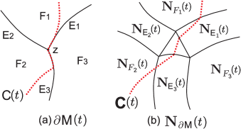
Figure 7: Curve of contact and normals of contact at time $t$

The left cap is defined as $L_{cap}=\{\gamma_{x}(t_{0})\in\partial M(t_{0})|\exists n\in N_{x}\mbox{ such that }g(x,n,t_{0})\leq 0\}$ and the right cap is defined as $R_{cap}=\{\gamma_{x}(t_{1})\in\partial M(t_{1})|\exists n\in N_{x}\mbox{ such that }g(x,n,t_{1})\geq 0\}$. The left cap and right cap are shown in the sweep example of Fig. 4. The left and right caps can be easily computed from the solid at initial and final positions.

Note that, by Proposition 9, ${\cal E}\subseteq L_{cap}\cup C\cup R_{cap}$. In general, a point on the contact set $C$ may not appear on the complete envelope ${\cal E}$ as it may get occluded by an interior point of the solid at a different time instant, see for example Fig. 20. This complicates the correct construction of the envelope by an appropriate trimming of the contact-set. We refer the reader to [4] for a comprehensive mathematical analysis of the trimming and the related subtle issues arising due to local/global intersections of the family $\{C(t)\}_{t\in I}$. In this paper, we focus on the case of simple sweeps.

Definition 11

A sweep $(M,h)$ is said to be simple if the envelope is the union of the contact set, the left cap and the right cap, i.e., ${\cal E}=L_{cap}\cup C\cup R_{cap}$.

Hence, in a simple sweep, every point on the contact set appears on the envelope and no trimming of the contact set is required in order to obtain the envelope.

Lemma 12

For a simple sweep, for $t\neq t^{\prime}$, $C(t)\cap C(t^{\prime})=\emptyset$. In short, no two distinct curves of contact intersect.

Refer to [5] for proof.

Definition 13

For a simple sweep, define the natural correspondence $\pi:C\to\partial M$ as follows: for $y\in C(t)$, we set $\pi(y)=x$ where $x$ is the unique point on $\partial M$ such that $\gamma_{x}(t)=y$.

Thanks to Lemma 12, $\pi$ is well-defined. Thus, $\pi(y)$ is the natural point on $\partial M$ which transforms to $y$ through the sweeping process.

Further, define the natural ‘normal’ correspondence ${\boldsymbol{\pi}}:{\bf C}\to{\bf N_{\partial M}}$ as ${\boldsymbol{\pi}}((y,n))=(x,n^{\prime})$ if $(y,n)=(\gamma_{x}(t),A(t)\cdot n^{\prime})$ for the unique $t\in I$ and the unique $(x,n^{\prime})\in{\bf N_{\partial M}}$ such that $g(x,n^{\prime},t)=0$ (cf. Proposition 9 and Definition 10).

The correspondence $\pi$ induces a natural brep structure on ${\cal E}$ which is derived from that of $\partial M$. The map $\pi$ is illustrated via color coding in the sweep examples shown in Figures 4, 8, 15 and 21 by showing the points $y$ and $\pi(y)$ in the same color.

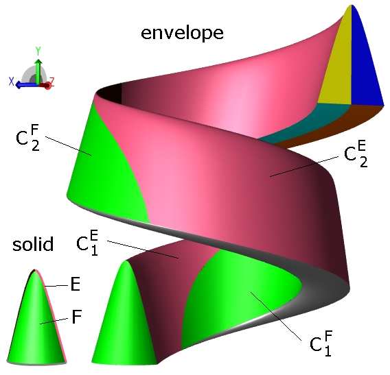
Figure 8: The sharp edge $E\subset\partial M$ generates two faces $C^{E}_{1}$ and $C^{E}_{2}$, all shown in pink. The face $F\subset\partial M$ generates two faces $C^{F}_{1}$ and $C^{F}_{2}$, all shown in green.

A face of $\partial M$ generates a set of faces on the contact set $C$. An edge or a vertex where $\partial M$ is G1-continuous generates a set of edges or vertices respectively on $C$. In other words, a G1-continuous subset $O$ of $\partial M$ generates entities on $C$ whose dimension is same as that of $O$. In the sweep example shown in Fig. 8, the face $F\subset\partial M$ generates a set of faces on $C$. However, a sharp edge of $\partial M$ generates a set of faces on $C$ and a sharp vertex generates a set of edges on $C$. This is illustrated in the example of Fig. 8 by the sharp edge labeled $E\subset\partial M$ which generates faces on $C$ shown in pink. For $O\subseteq\partial M$, we denote the contact set generated by $O$ by $C^{O}$, i.e., $C^{O}=\{y\in C|\pi(y)\in O\}$. Note that while $O$ is connected, the corresponding contact set $C^{O}$ may not be. A connected component of $C^{O}$ is denoted using a subscript, for example, faces $C^{E}_{1}$ and $C^{E}_{2}$ in Fig. 8 correspond to the edge $E\subset\partial M$.

3 The computational framework

Algorithm 1 given below provides an outline of the basic Algorithm 1 of [5] and its extension to sharp edges, which begins on Step 14, and which is the main contribution of the paper.

Algorithm 1 Solid sweep

1:for all faces $F$ in $\partial M$ do

2:     for all co-edges $c$ in $\partial F$ do

3:         for all $z$ in $\partial c$ do

4:              Compute vertices $C^{z}$ generated by $z$

5:         end for

6:         Compute co-edges $C^{c}$ generated by $c$

7:         Orient co-edges $C^{c}$

8:     end for

9:     Compute $C^{F}(t_{0})$ and $C^{F}(t_{1})$

10:     Compute loops bounding faces $C^{F}$ which will be generated by $F$

11:     Compute faces $C^{F}$ generated by $F$

12:     Orient faces $C^{F}$

13:end for

14:for all sharp edges $E$ in $\partial M$ do

15:     for all $Z$ in $\partial E$ do

16:         Compute co-edges $C^{Z}$ generated by $Z$

17:         Orient co-edges $C^{Z}$

18:     end for

19:     $(F,F^{\prime})\leftarrow AdjacentFaces(E)$

20:     Compute co-edges $C^{E}\cap C^{F}$ and $C^{E}\cap C^{F^{\prime}}$

21:     Orient co-edges $C^{E}\cap C^{F}$ and $C^{E}\cap C^{F^{\prime}}$

22:     Compute $C^{E}(t_{0})$ and $C^{E}(t_{1})$

23:     Compute loops bounding faces $C^{E}$ which will be generated by $E$

24:     Compute faces $C^{E}$ generated by $E$

25:     Orient faces $C^{E}$

26:end for

27:Compute adjacencies between faces of $C$

We outline what was achieved in [5]. At the heart of Algorithm 1 is an entity-wise implementation of the correspondence $\pi$ which is a classification of the faces, edges and vertices of ${\cal E}$ by the generating entity in $\partial M$. This is achieved by computing $C^{O}$ of the envelope for key entities $O\subseteq\partial M$ which yield faces in ${\cal E}$. The smooth case is easy since faces generate faces, edges generate edges and so on. The computation of $C^{O}$ is followed by an orientation calculation. It was noted that while the adjacencies of entities in ${\cal E}$ were built from that on $\partial M$, the orientation on ${\cal E}$ was not as on $\partial M$ and in fact could be positive, negative or zero vis a vis that on $\partial M$.

Let us outline the details of the computation of $C^{F}$ for a smooth face $F\subseteq\partial M$. Suppose that $F$ is given by the parametrization $S:D\rightarrow\mathbb{R}^{3}$, where $D$ is a domain in $\mathbb{R}^{2}$ with parameters $(u,v)$. Let $I$ be the interval used to parametrize the motion $h$. The envelope condition (cf. Proposition 5) yields a function $f^{F}(u,v,t)$ on the prism $D\times I$, viz., $f^{F}(u,v,t)=\langle A(t)\cdot N(u,v),\gamma_{S(u,v)}^{\prime}(t)\rangle$ where $N(u,v)$ is the outward normal to $F$ at $S(u,v)$. For simple sweeps $f^{F}(u,v,t)=0$ indicates that $A(t)\cdot S(u,v)+b(t)$ is on the envelope. This led to the definition of the funnel ${\cal F}^{F}$ as the zero-set of $f^{F}$ within the prism. If ${\cal F}^{F}_{1},\ldots,{\cal F}^{F}_{k}$ are the connected components of the funnel then (i) the face $F$ leads to exactly $k$ disjoint faces $C^{F}_{1},\ldots,C^{F}_{k}$ in the envelope ${\cal E}$, (ii) each ${\cal F}^{F}_{i}$ serves as the parameter space to implement $C^{F}_{i}$, (iii) the boundary of ${\cal F}^{F}_{i}$ arises from ${\cal F}^{F}$ intersecting the boundary of the prism and parametrizes the co-edges of $C^{F}_{i}$. The above computation is achieved in Steps 1 to 13 of Algorithm 1.

The same approach works when the solid has sharp features, albeit with some complications. Firstly, a sharp edge generates a face and a sharp vertex an edge. This is because, for a point $x$ on a sharp edge, there is actually a cone of normals $N_{x}$ (cf. Definition 6). Whence $\gamma_{x}(t)$ is on the envelop ${\cal E}$ iff the velocity $\gamma_{x}^{\prime}(t)$ is perpendicular to any element of $A(t).N_{x}$ (cf. Proposition 9). Thus, this results in the sharp edge $E$ in extruding a 2-dimensional entity. The analysis of the smooth face via the prism and the funnel lifts easily and naturally to the case of the sharp edge $E$. The prism is ${\bf N_{E}}\times I$, suitably parametrized, which is a $3$-dimensional entity. The envelope condition leads to an implicit surface pre-funnel. The funnel ${\cal F}^{E}$ is the projection of the pre-funnel on to $E\times I$. Thus, for a point $x\in E$ and $t\in I$, if $(x,t)\in{\cal F}^{E}$, then $\gamma_{x}(t)$ is on the envelope. See Fig. 9 for an illustration of how funnels of smooth faces interact with the pre-funnel of the sharp edge.

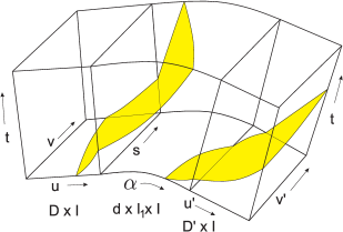
Figure 9: Prisms for faces $F,F^{\prime}$ and edge $E$ shown adjacent to each other. The funnels of $F,F^{\prime}$ and pre-funnel of $E$ are shaded in yellow.

The geometry of $C^{E}$ is simpler: it is merely the geometry of a translate/sweep of a curve and is implemented routinely in most kernels. Further, the orientation of a face of $C^{E}$ is also shown to be easily computable.

The trims/boundary of a face of $C^{E}$ is obtained by examining the components of ${\cal F}^{E}$ whose boundaries are shown to be intimately related to the normal cones. Next, for a sharp vertex $Z$, it is easy to compute a set of sub-intervals of $I$ when appropriate translates of $Z$ will appear as edges on ${\cal E}$. The computation of adjacencies between the new entities is governed by a simple yet rich interplay between the normal cones at sharp points and their trajectories.

The key technical contributions thus are essentially (i) a calculus of the sweep of normal cones and its embedding into a brep framework (ii) a seamless architectural integration of sharp features into the general solid sweep framework. An obvious question is why it could not have been done before, i.e., in [5] itself. The answer is of course that the structure of sweeps $C^{F}$ of smooth faces is the key construct and the $C^{E}$, i.e., sweeps of sharp edges are essentially transition faces. Thus the theory of these transition faces must be subsequent to that of the smooth faces.

4 Calculus of cones

In this section we develop the mathematics of the interaction between the cones at sharp points and their trajectories under $h$.

Towards this, fix a sharp point $x$ with normal cone $N_{x}$ and a time instant $t$. Proposition 9 provides a geometric condition which determines if $\gamma_{x}(t)$ will be on ${\cal E}$. Namely, $\gamma_{x}(t)\in{\cal E}$ iff there exists $n\in N_{x}$ such that $g(x,n,t)=\left<\gamma_{x}^{\prime}(t),A(t).n\right>=0$.

Further, if $n_{1},n_{2}\in N_{x}$ are such that $g(x,n_{1},t)=g(x,n_{2},t)=0$ then for any linear combination $n\in N_{x}$ of $n_{1}$ and $n_{2}$, $g(x,n,t)=0$. This follows by observing that, having fixed $x$ and $t$, the function $g(x,n,t)$ is linear in $n$.

4.1 Interaction between $N_{x}$ and $\gamma_{x}(t)$ on a sharp edge

Consider a sharp edge $E$ bounding the smooth faces $F,F^{\prime}$ in $\partial M$. Further, fix an interior point $x$ on $E$ and a time instant $t$. Let $N_{1}$ and $N_{2}$ be the unique unit outward normals to $F$ and $F^{\prime}$ at $x$. Note that that the normal cone $N_{x}$ is ‘spanned’ by $N_{1}$ and $N_{2}$.

Let $\bar{w}$ be the tangent to $E$ at $x\in E$. Clearly, for every $n\in N_{x}$, $\left<n,\bar{w}\right>=0$ and thus, $\left<A(t)\cdot n,A(t)\cdot\bar{w}\right>=0$. Now $\left<\gamma_{x}^{\prime}(t),A(t)\cdot n\right>=0$ for some $n\in N_{x}$ iff $A(t)\cdot n$ is parallel to $A(t)\cdot\bar{w}\times\gamma_{x}^{\prime}(t)$. Hence, $\gamma_{x}(t)\in{\cal E}$ if and only if $A(t)\cdot\bar{w}\times\gamma_{x}^{\prime}(t)\in A(t)\cdot N_{x}$ or $-A(t)\cdot\bar{w}\times\gamma_{x}^{\prime}(t)\in A(t)\cdot N_{x}$. This is illustrated schematically in Figure 10.

Further, note that, if $\gamma_{x}(t)\in{\cal E}$ then we have the following dichotomy: either there exists a unique $n\in N_{x}$ such that $g(x,n,t)=0$ or for all $n\in N_{x}$ $g(x,n,t)=0$. It is easy to see that the later condition is equivalent to $A(t)\cdot\bar{w}\times\gamma_{x}^{\prime}(t)=\bar{0}$ and as shown in Section 5.2 leads to a singularity on $C^{E}$.

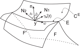
Figure 10: The cone of unit normals at $N_{x}$ formed by normals $N_{1}$ and $N_{2}$ to faces $F$ and $F^{\prime}$ respectively meeting in sharp edge $E$.

For further discussion, we assume without loss of generality that $A(t)=I$ and $b(t)=0$. Define $N_{x}^{-}=\{\bar{z}\in\mathbb{R}^{3}|\left<n,\bar{z}\right><0\ \forall n\in N_{x}\}$ and $N_{x}^{+}=\{\bar{z}\in\mathbb{R}^{3}|\left<n,\bar{z}\right>>0\ \forall n\in N_{x}\}$. $N_{x}^{-}$ and $N_{x}^{+}$ are illustrated schematically in Figure 11. By Proposition 9, $\gamma_{x}^{\prime}(t)\in N_{x}^{+}\cup N_{x}^{-}$ iff $\gamma_{x}(t)\notin{\cal E}$. The complement of $N_{x}^{+}\cup N_{x}^{-}$ is shaded in yellow in Figure 11. It is easy to see that, $\gamma_{x}(t)\in{\cal E}$ if and only if either (i) $\left<N_{1},\gamma_{x}^{\prime}(t)\right>\leq 0$ and $\left<N_{2},\gamma_{x}^{\prime}(t)\right>\geq 0$ or (ii) $\left<N_{1},\gamma_{x}^{\prime}(t)\right>\geq 0$ and $\left<N_{2},\gamma_{x}^{\prime}(t)\right>\leq 0$. This condition is computationally easy to check and is used to define the trim curves of $C^{E}$.

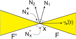
Figure 11: The point $\gamma_{x}(t)$ is on contact set if and only if $\gamma_{x}^{\prime}(t)$ is in the region shaded in yellow.

4.2 Interaction between $N_{x}$ and $\gamma_{x}(t)$ at a sharp vertex

Consider now the case when $x$ is a vertex with face normals $N_{1},N_{2},N_{3}$ coming from faces $F_{1},F_{2},F_{3}$ respectively. As before, for simplicity, we assume that $A(t)=I$ and $b(t)=0$.

Once again, $\gamma_{x}(t)\in{\cal E}$ iff there is an $n\in N_{x}$ such that $\langle n,\gamma_{x}^{\prime}(t)\rangle=0$. Figure 12 schematically illustrates the set $\{n\in N_{x}|\left<n,\gamma_{x}^{\prime}(t)\right>=0\}$ of normals of contact at time $t$. An important observation is that this set is closed under linear combinations. Therefore, upto permutations of $N_{i}$’s, Figure 12 describes all the configurations which lead to $\gamma_{x}(t)\in{\cal E}$.

It is also clear that the condition that $\gamma_{x}(t)\in{\cal E}$ reduces to $\left<N_{i},\gamma_{x}^{\prime}(t)\right>\leq 0$ and $\left<N_{j},\gamma_{x}^{\prime}(t)\right>\geq 0$ for some $i,j\in\{1,2,3\}$ which is computationally benign.

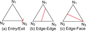
Figure 12: Three possible configurations of the normals of contact at $t$ for sharp vertex $Z$. The set $\{n\in N_{Z}|\left<n,\gamma_{z}^{\prime}(t)\right>=0\}$ is shown as a dotted curve in red in ${\bf N_{Z}}$.

5 Parametrization and Geometry of $C^{E}$ and $C^{Z}$

In this section we describe the parametrization and geometry of the faces and edges of $C$ generated by sharp features of $\partial M$ and the detection of singularities in these. We extend the key constructs of prism and funnel proposed in [5] for smooth faces of $\partial M$ to the sharp features of $\partial M$. The funnel serves as the parameter space for faces of $C^{E}$ and guides further computation of the envelope.

Recall that a (smooth and non-degenerate) face is a map $S:D\rightarrow\mathbb{R}^{3}$, where $D\subseteq\mathbb{R}^{2}$ is a domain bounded by trim curves. A smooth parametric curve in $\mathbb{R}^{3}$ is a (smooth and non-degenerate) map $e:d\to\mathbb{R}^{3}$ where $d=[s_{0},s_{1}]$ is a closed interval of $\mathbb{R}$. Thus, specifying a face (resp. edge) requires us to specify the functions $S$ (resp. $e$) and the domain $D$ (resp. $d$).

5.1 Parametrization of faces $C^{E}$

Let $E$ be a sharp edge of $\partial M$ supported by two faces $F$ and $F^{\prime}$. Let $e$ be the curve underlying the sharp edge $E$ and $d$ be the subset of the parameter space of $e$ corresponding to $E$, i.e., $e(d)=E$. We extend the notion of prism proposed in [5] for smooth faces of $\partial M$ to the edge $E$. At every point $e(s)\in E$, we may parametrize the cone of unit normals $N_{e(s)}$ as $N_{e(s)}(\alpha)=\frac{\alpha\cdot N_{1}+(1-\alpha)\cdot N_{2}}{\|\alpha\cdot N_{1}+(1-\alpha)\cdot N_{2}\|}$ for $\alpha\in I_{1}=[0,1]$, where, $N_{1}$ and $N_{2}$ are the unit outward normals to $F$ and $F^{\prime}$ respectively at point $e(s)$. We refer to the subset $d\times I_{1}\times I$ of $\mathbb{R}^{3}$ as the prism of $E$. A point $(s,\alpha,t)$ in the prism corresponds to the normal $A(t)\cdot N_{e(s)}(\alpha)$ at the point $\gamma_{e(s)}(t)$ in the unit normal bundle ${\bf N_{E}}(t)$. Define the real-valued function $f^{E}$ on the prism of $E$ as $f^{E}(s,\alpha,t)=g(e(s),N_{e(s)}(\alpha),t)$. Clearly if $f^{E}(s,\alpha,t)=0$ then $\gamma_{e(s)}(t)\in C^{E}$. This motivates us to define the funnel as the projection of the zero-set of $f^{E}$ above to $d\times I$, as follows:

Definition 14

For a sweep interval $I$ and a sharp edge $E\subset\partial M$, define ${\cal F}^{E}=\{(s,t)\in d\times I|f^{E}(s,\alpha,t)=0\mbox{ for some }\alpha\in I_{1}\}$. The set ${\cal F}^{E}$ is referred to as the funnel for $E$. The set $\{(s,t)\in{\cal F}^{E}|t=t^{\prime}\}$ is referred to as the p-curve of contact at $t^{\prime}$ and denoted by ${\cal F}^{E}(t^{\prime})$.

The set ${\cal F}^{E}$ serves as the domain of parametrization for the faces $C^{E}$ generated by $E$. The parametrization function is given by $\sigma^{E}:{\cal F}^{E}\to\mathbb{R}^{3}$ as $\sigma^{E}(s,t)=A(t)\cdot e(s)+b(t)$.

It now remains to compute the trim curves of ${\cal F}^{E}$. We now assume for simplicity the zero-set of $f^{E}$ is bounded by the boundaries of the prism $d\times I_{1}\times I$. Thus the boundaries of ${\cal F}^{E}$ come from the equations $s=s_{0},s_{1}$ or $t=t_{0},t_{1}$ or finally $\alpha=0,1$. The first two conditions are easily implemented. The condition $\alpha=0$ is equivalent to the assertion that $a^{E}_{1}(s,t)=\langle A(t)\cdot N_{1}(e(s)),\gamma_{e(s)}^{\prime}(t)\rangle=0$ , where $N_{1}(e(s))$ is the normal to the face $F$ at the point $e(s)$. The function $a^{E}_{1}(s,t)=0$ and the similarly defined $a^{E}_{2}(s,t)=0$ (for face $F^{\prime}$) serve as the final trim curves. This collection of trim curves may yield several components, each corresponding to a unique face of $C^{E}$ on ${\cal E}$.

Fig. 13(a) illustrates the funnel ${\cal F}^{E}$ shaded in yellow and p-curves of contact ${\cal F}^{E}(t^{\prime}),{\cal F}^{E}(t^{\prime\prime})$ and ${\cal F}^{E}(t^{\prime\prime\prime})$ shown in red. In this example, ${\cal F}^{E}$ has two connected components. The curves $\sigma^{E}({\cal F}^{E}(t))$ are parts of the curve of contact on ${\cal E}$ at time $t$. In Fig. 13(b), the normals of contact, i.e., $A(t)\cdot e^{\prime}(s)\times\gamma_{x}^{\prime}(t)$ at times $t^{\prime},t^{\prime\prime}$ and $t^{\prime\prime\prime}$ are shown projected on the unit normal bundle ${\bf N_{E}}$.

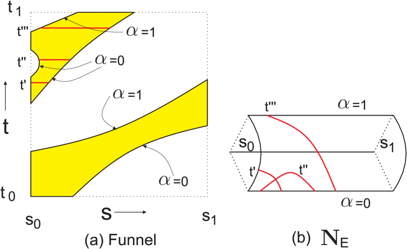
Figure 13: (a) The funnel ${\cal F}^{E}$ is shaded in yellow. The p-curves of contact at $t^{\prime},t^{\prime\prime}$ and $t^{\prime\prime\prime}$ are shown in red. (b) The curves ${\boldsymbol{\pi}}({\bf C}(t^{\prime})),{\boldsymbol{\pi}}({\bf C}(t^{\prime\prime}))$ and ${\boldsymbol{\pi}}({\bf C}(t^{\prime\prime\prime}))$ are shown on ${\bf N_{E}}$.

5.2 Singularities in $C^{E}$

A parametric surface $S$ is said to have a singularity at a point $S(u_{0},v_{0})$ if $S$ fails to be an immersion at $(u_{0},v_{0})$, i.e., the rank of the Jacobian $J_{S}$ falls below 2.

Lemma 15

Let $p=(s^{\prime},t^{\prime})\in{\cal F}^{E}$. A face of $C^{E}$ has a singularity at point $\sigma^{E}(p)$ if and only if the velocity $\gamma_{e(s^{\prime})}^{\prime}(t^{\prime})$ is tangent to the edge $E$ at the point $\sigma^{E}(p)$, i.e., $\gamma_{e(s^{\prime})}^{\prime}(t^{\prime})$ and $A(t^{\prime})\cdot\frac{de}{ds}(s^{\prime})$ are linearly dependent.

Fig. 14 illustrates schematically a funnel ${\cal F}^{E}$ having a singularity at $t^{\prime\prime}$. A sweep example with singularity is shown in Fig. 15.

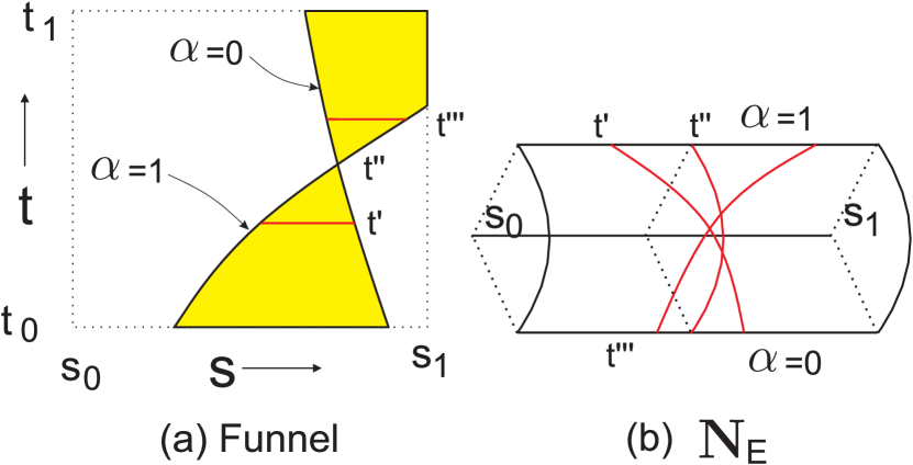
Figure 14: Singularity in $C^{E}$. (a) The funnel is shaded in yellow. The p-curves of contact ${\cal F}^{E}(t^{\prime}),{\cal F}^{E}(t^{\prime\prime})$ and ${\cal F}^{E}(t^{\prime\prime\prime})$ are shown in red. (b) The curves ${\boldsymbol{\pi}}({\bf C}(t^{\prime})),{\boldsymbol{\pi}}({\bf C}(t^{\prime\prime}))$ and ${\boldsymbol{\pi}}({\bf C}(t^{\prime\prime\prime}))$ are shown on ${\bf N_{E}}$.

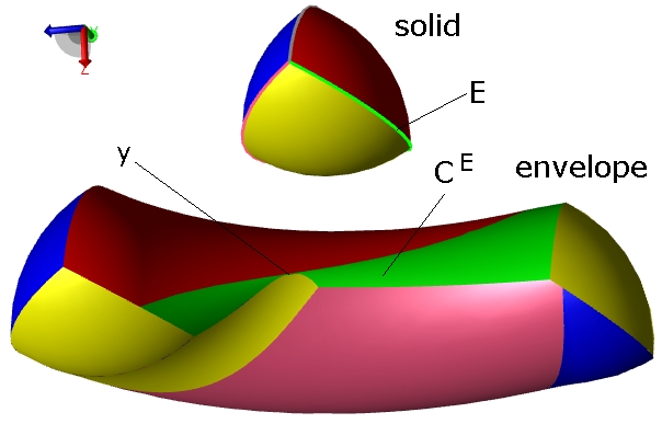
Figure 15: The contact set $C^{E}$ has a singularity at point $y$.

5.3 Parametrization of edges $C^{Z}$

Let $Z$ be a sharp vertex lying in the intersection of faces $F_{1},F_{2}$ and $F_{3}$ and let $N_{1},N_{2}$ and $N_{3}$ be the unit outward normals to $F_{1},F_{2}$ and $F_{3}$ respectively at $Z$. As noted in Section 4, the point $\gamma_{Z}(t)$ belongs to the contact set $C^{Z}$ if and only if $\left<A(t)\cdot N_{i},\gamma_{Z}^{\prime}(t)\right>\leq 0$ and $\left<A(t)\cdot N_{j},\gamma_{Z}^{\prime}(t)\right>\geq 0$ for some $i,j\in\{1,2,3\}$. Define functions $s_{i}:I\to\mathbb{R}$ as $s_{i}(t)=\left<A(t)\cdot N_{i},\gamma_{Z}^{\prime}(t)\right>$ for $i=1,2,3$. Clearly, the contact set $C^{Z}$ corresponds to the set of closed sub-intervals of the sweep interval $I$ where any two of the functions $s_{i}$ differ in sign. This is illustrated schematically in Fig. 16. At the end-points of these sub-intervals, either $t\in\{t_{0},t_{1}\}$ (illustrated by points $a$ and $f$ in Fig. 16) or one of the functions $s_{i}$ is zero (illustrated by points $b,c,c^{\prime},d$ and $e$ in Fig. 16). Thus the collection of sub-intervals $d_{Z}$ of $I$ is easily computed. The parametrization function of course is $\gamma_{Z}:d_{Z}\rightarrow\mathbb{R}^{3}$ given by the trajectory of the point $Z$ under $h$. This finishes the parametrization of $C^{Z}$.

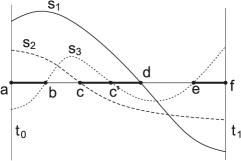
Figure 16: The functions $s_{1}$, $s_{2}$ and $s_{3}$ are plotted against time.

6 Adjacencies and topology of $C$

We now focus on the matching of co-edges for each face of $C$. We already know that faces of $C$ come from (i) $C^{E}$ when $E$ is a sharp edge, or (ii) $C^{F}$ when $F$ is a smooth face. Similarly edges in $C$ come from (i) edges bounding faces of $C^{E},C^{F}$ and (ii) edges coming from $C^{Z}$, where $Z$ is a sharp vertex. The matching of co-edges is eased by the following proximity lemma. While the global brep structure of $C$ may be very different from that of $\partial M$, we show that locally they are similar.

Recall the natural correspondence ${\pi}:{C}\to{{\partial M}}$ from Section 2. We show that the adjacency relations between geometric entities of $C$ are preserved by the correspondence $\pi$.

Lemma 16

The correspondence map $\pi:C\to\partial M$ is continuous.

Proof. For a face $F\subseteq M$, we denote the restriction of the map ${\pi}$ to ${C^{F}}$ by $\pi^{F}$, i.e., $\pi^{F}:C^{F}\to F$, $\pi^{F}(y)=\pi(y)$. The restriction of ${\pi}$ to ${C^{E}}$ for a sharp edge $E\subset\partial M$ is defined similarly. Consider first the restriction $\pi^{E}$ of $\pi$ to $C^{E}$. Recall the parametrization of $C^{E}$ via the funnel ${\cal F}^{E}$ and $\sigma^{E}$ from Section 5.1. Let $y\in C^{E}$ and $p=(s^{\prime},t^{\prime})\in{\cal F}^{E}$ such that $\sigma^{E}(p)=y$. The map $\sigma^{E}$ being continuous, in order to show that $\pi^{E}$ is continuous at $y$, it is sufficient to show that the composite map $\pi^{E}\circ\sigma^{E}:{\cal F}^{E}\to E$ given by $\pi^{E}\circ\sigma^{E}(s,t)=e(s)$ is continuous at $p$, where, $e$ is the parametric curve underlying edge $E$. This follows from the continuity of $e$.

The continuity of the restriction $\pi^{F}$ to $C^{F}$ for a face $F\subseteq\partial M$ can be similarly proved, by choosing a pair of local coordinates at any point $p\in{\cal F}^{F}$.

The continuity of the map $\pi$ follows from the fact that $\pi$ is obtained by gluing the maps $\{\pi^{F}|F\subseteq M\}\cup\{\pi^{E}|E\mbox{ is a sharp edge in }\partial M\}$ each of which is continuous. $\square$

We conclude the following theorem from the above proposition.

Theorem 17

For any two geometric entities $O$ and $O^{\prime}$ of $\partial M$, if $C^{O}$ and $C^{O^{\prime}}$ are adjacent in $C$, then $O$ and $O^{\prime}$ are adjacent in $\partial M$.

In other words, for a face $F\subset\partial M$ and a sharp edge $E\subset\partial M$, if faces $C^{F}_{i}$ and $C^{E}_{j}$ are adjacent in $C$, then $F$ and $E$ are adjacent in $\partial M$. For a sharp vertex $Z\subset\partial M$, if an edge $C^{Z}_{k}$ bounds a face $C^{E}_{j}$ in $C$ then the vertex $Z$ bounds the edge $E$ in $\partial M$.

This aids the computation of adjacency relations amongst entities of $C$ and is illustrated by the sweep example shown in Figures 4, 8, 15 and 21 by color coding. The entities $O$ and $C^{O}$ are shown in same color.

6.1 Co-edges bounding faces $C^{E}$

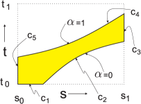
Figure 17: Co-edges bounding face $C^{E}$.

Consider a sharp edge $E$ supported by smooth faces $F$ and $F^{\prime}$ in $\partial M$. We pick a face of $C^{E}$ given by the component of ${\cal F}^{E}$ shown in Fig. 17. The co-edges $c_{5},c_{3}$ come from the equations $s=s_{0}$ and $s=s_{1}$ respectively. These must correspond to edges swept by sharp vertices bounding the edge $E$. The co-edge $c_{1}$ comes from the condition $t=t_{0}$ and thus comes from curve of contact at the initial time instant and thus, the left cap. Finally, the curves $c_{2},c_{4}$ correspond to $a^{E}_{1}(s,t)=0$ and $a^{E}_{2}(s,t)=0$ which come from the normals of contact matching that of the supporting smooth faces as described in Section 5. Thus these co-edges must match those coming from the boundaries of $C^{F}$ and $C^{F^{\prime}}$.

6.2 Co-edges matching edges of $C^{Z}$

We next come to the co-edges matching with edges arising from $C^{Z}$. As in Fig. 16, the edges of $C^{Z}$ are parametrized by intervals $d_{1},\ldots,d_{k}$. Each interval $d_{i}$ has two of the three functions $s_{1},s_{2}$ and $s_{3}$ of one sign and the third of the opposite sign. For example, if we take the interval $(c,c^{\prime})$, we see that $s_{1},s_{3}>0$ and $s_{2}<0$. For $t\in(c,c^{\prime})$, if we look at the zero locus of the function $\langle A(t)\cdot n,\gamma_{Z}^{\prime}(t)\rangle$, on $N_{Z}$, then there must be an $n_{1}\in cone(N_{1},N_{2})\subset N_{Z}$ such that $\langle A(t)\cdot n_{1},\gamma_{Z}^{\prime}(t)\rangle=0$ and there must be an $n_{2}\in cone(N_{2},N_{3})\subset N_{Z}$ such that $\langle A(t)\cdot n_{2},\gamma_{Z}^{\prime}(t)\rangle=0$. This leads us to the sharp edge $E_{1}$ with normals $N_{1},N_{2}$ at the vertex $Z\in E_{1}$, and to the sharp edge $E_{2}$ with normals $N_{3},N_{2}$ at $Z\in E_{2}$ and the conclusion that that faces of $C^{E_{1}}$ and $C^{E_{2}}$ meet at the edge $[c,c^{\prime}]$ of $C^{Z}$. See for example, the curve of contact $C(t^{\prime})$ in Fig. 18. A similar conclusion for the interval $(c^{\prime},d)$ tells us that faces of $C^{E_{1}}$ and $C^{E_{3}}$ meet on the edge $[c^{\prime},d]$ of $C^{Z}$. The curious point is the time instant $c^{\prime}$ where the smooth face $F_{3}$ with normal $N_{3}$ also meets the edge $C^{Z}$. This is illustrated by curve of contact $C(t^{\prime\prime})$ in Fig. 18 where there are four incident faces.

Figure 18: Adjacency relations between faces of $C$. (a) Solid being swept. (b) Normals of contact ${\boldsymbol{\pi}}({\bf C}(t))$, ${\boldsymbol{\pi}}({\bf C}(t^{\prime}))$ and ${\boldsymbol{\pi}}({\bf C}(t^{\prime\prime}))$ are shown on the unit normal bundle ${\bf N_{\partial M}}$. (c) Curves of contact $C(t)$, $C(t^{\prime})$ and $C(t^{\prime\prime})$ are shown in red. The edge $C^{Z}$ generated by the sharp vertex $Z\subset\partial M$ is shown as a dotted curve in black on $C$.

7 Computation of the brep of $C$

In this section we explain Steps 14 to 27 of Algorithm 1 for generating the entities on the envelope corresponding to sharp edges and vertices of $\partial M$. Algorithm 1 marches over each entity $O$ of $\partial M$ and computes the corresponding entity $C^{O}$ of $C$. The computation of $C^{O}$ follows the computation of its boundary $\partial C^{O}$. For further discussion fix a sharp edge $E$ of $\partial M$ (cf Step 14 of Algorithm 1).

7.1 Computing and orienting co-edges $C^{Z}$

Consider a sharp vertex $Z\subset\partial E$. Recall from Section 5.3 that computing the edges $C^{Z}$ is equivalent to computing the collection of closed subintervals of the sweep interval $I$ in which the functions $s_{i}$ differ in sign. We use Newton-Raphson solvers for computing the end-points of these subintervals. Of course, these end-points give rise to vertices which bound edges of $C^{Z}$. This is performed in Step 16 of Algorithm 1.

Each co-edge $C^{Z}_{i}$ bounding the face $C^{E}_{j}$ must be oriented so that $C^{E}_{j}$ is on its left side with respect to the outward normal in a right-handed co-ordinate system. Let $y=\gamma_{Z}(t)\in C^{Z}_{i}$ and $\bar{w}\in\mathbb{R}^{3}$ be tangent to $C^{Z}_{i}$ at $y$. Let $n$ be the outward unit normal to $C^{E}_{j}$ at $y$ (cf Section 7.4). Assume without loss of generality that $A(t)=I$ and $b(t)=0$. Let $e$ be the parametric curve underlying $E$ so that $e(d)=E$ where $d=[s_{0},s_{1}]$. Consider two cases as follows.

1. If $Z=e(s_{0})$, then $e^{\prime}(s_{0})$ points in the interior of the face $C^{E}_{j}$, where, $e^{\prime}$ denotes the derivative of $e$. If $\left<e^{\prime}(s_{0}),n\times\bar{w}\right>>0$ then $\bar{w}$ is the orientation of $C^{Z}_{i}$ else $-\bar{w}$ is the orientation.

2. If $Z=e(s_{1})$ then $-e^{\prime}(s_{1})$ points in the interior of $C^{E}_{j}$. If $\left<-e^{\prime}(s_{1}),n\times\bar{w}\right>>0$ then $\bar{w}$ is the orientation of $C^{Z}_{i}$ else $-\bar{w}$ is the orientation. This is illustrated schematically in Fig. 19.

The co-edges $C^{Z}$ are oriented in Step 17 of Algorithm 1.

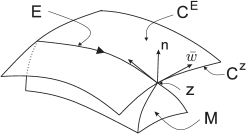
Figure 19: Orienting co-edges $C^{Z}$. In this case $e(s_{1})=Z$ and $-e^{\prime}(s)|_{s_{1}}$ points in the interior of face $C^{E}$.

7.2 Computing and orienting co-edges $C^{E}\cap C^{F}$ and $C^{E}\cap C^{F^{\prime}}$

For the sharp edge $E$ supported by smooth faces $F$ and $F^{\prime}$ in $\partial M$, the co-edges $C^{E}\cap C^{F}$ and $C^{E}\cap C^{F^{\prime}}$ bounding a face of $C^{E}$ correspond to the iso-$\alpha$ curves for $\alpha\in\{0,1\}$ of $C^{E}$ as discussed in Section 6.1. The orientation of these co-edges for $C^{E}$ is opposite to that of the partner co-edges for $C^{F}$ and $C^{F^{\prime}}$. The co-edges bounding $C^{F}$ and $C^{F^{\prime}}$ are computed and oriented in Steps 6 and 7 of Algorithm 1. Their partner co-edges bounding faces $C^{E}$ are computed and oriented in Step 20 and 21 of Algorithm 1.

7.3 Computing loops bounding faces $C^{E}$

A loop is a closed, connected sequence of oriented co-edges which bound a face. As noted in Section 6.1, the co-edges bounding faces of $C^{E}$ are either iso-$\alpha$ curves for $\alpha\in\{0,1\}$, or iso-$s$ curves for $s\in\{s_{0},s_{1}\}$ or iso-$t$ curves for $t\in\{t_{0},t_{1}\}$. In order to compute the loop bounding a face $C^{E}_{i}$, we start with a co-edge bounding $C^{E}_{i}$ and find the next co-edge in sequence. For instance, if this co-edge is iso-$\alpha$ curve for $\alpha=0$ and its end-point is $(\alpha,s)=(0,s_{1})$ then the next co-edge in sequence is iso-$s$ curve with $s=s_{1}$. This is repeated till the loop is closed. Fig. 17 illustrates this schematically. This computation is performed in Step 23 of Algorithm 1.

7.4 Computing and orienting faces $C^{E}$

The parametrization of faces $C^{E}$ was discussed in Section 5.1 via the funnel ${\cal F}^{E}$. This is done in Step 24 of Algorithm 1. Each face in the brep format is oriented so that the unit normal to the face points in the exterior of the solid. Consider a point $y=\gamma_{z}(t)\in C^{E}$ and assume without loss of generality that $A(t)=I$ and $b(t)=0$. Recall from Section 4.1 and Section 5.1 that if $\bar{w}$ is tangent to $E$ at $z$, then $n:=A(t)\cdot\bar{w}\times\gamma_{z}^{\prime}(t)$ is normal to $C^{E}$. Further, either $n\in A(t)\cdot N_{z}$ or $-n\in A(t)\cdot N_{z}$. Since the interior of the swept volume is ${\cal V}^{o}=\cup_{t\in I}M(t)^{o}$, the outward normal to $C^{E}$ at $y$ is $n$ if $n\in A(t)\cdot N_{z}$ else it is $-n$. This is performed in Step 25 of Algorithm 1.

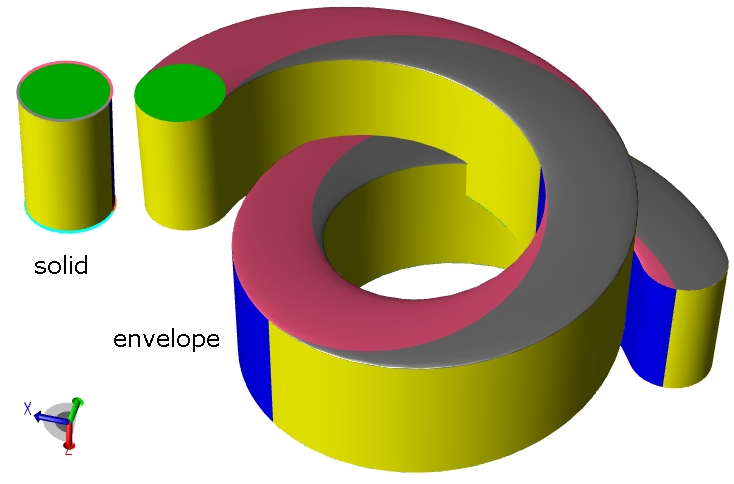
Figure 20: An example illustrating global self-intersection.

Our framework is tested on over 50 different solids with number of sharp edges and smooth faces between 4 and 25, swept along complex trajectories. A pilot implementation using the ACIS [3] kernel took between 30 seconds to 2 minutes on a Dual Core 1.8 GHz machine for these examples, some of which appear in Fig. 21. Many more examples are included in the supplementary file.

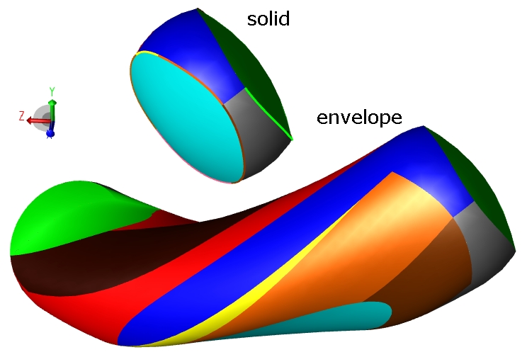
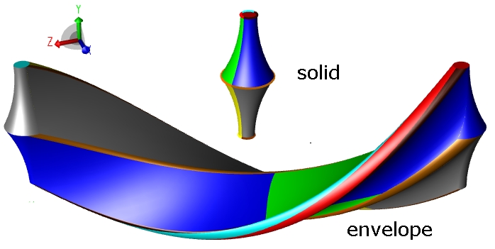
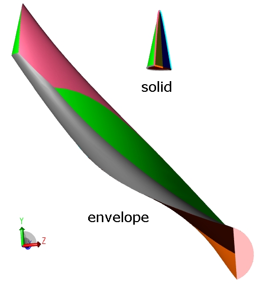
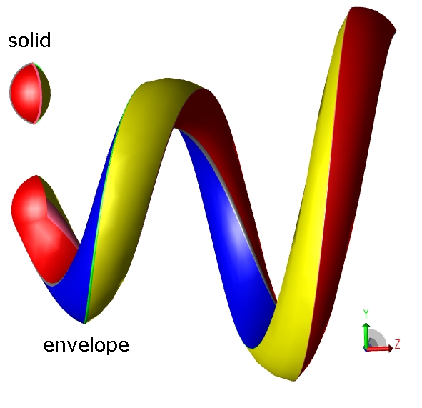
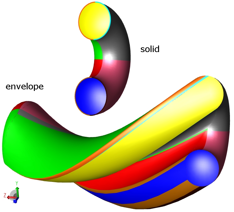
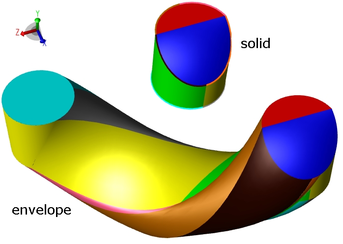
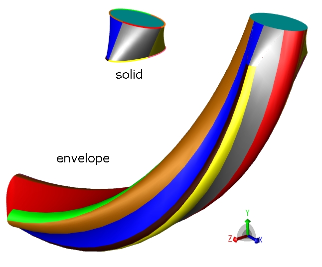
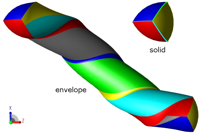
Figure 21: Examples of solid sweep

8 Extension to non-simple sweeps

In this section, we discuss an extension of the above framework to ‘non-simple’ sweeps. Recall that, in a non-simple sweep, the correct construction of the envelope proceeds with an appropriate trimming of the contact set. This calls for local and global self-intersections of the contact set (see [7, 19, 4] for definitions). Global self-intersections may be resolved by surface-surface intersections, which is a standard routine in modern CAD kernels. A sweep example with global self-intersection appears in Fig. 20. Local self-intersections are more subtle. Roughly speaking, in a local self-intersection, a point on the contact set is occluded by an infinitesimally close point.

In [4], the authors assume that the input solid is smooth and construct an invariant function $\theta$ on the contact set which efficiently separates global self-intersections from local self-intersections. The function $\theta$ is intimately related to local curvatures and the inverse trajectory (see [7, 9]) used in earlier works. Further, it has been shown there that $\theta$ is robust and provides the key ‘seed‘ information to resolve local self-intersections via surface-surface intersections. Much of this work also extends to sharp solids albeit restricted to only the part of the contact set which is generated by smooth features. Clearly, it is important to understand the self-intersections on the contact set generated by sharp features. We next show that the sharp features never give rise of local self-intersections!

Definition 18

Given a trajectory $h$, the inverse trajectory $\bar{h}$ is defined as the map $\bar{h}:I\to(SO(3),\mathbb{R}^{3})$ given by $\bar{h}(t)=(A^{t}(t),-A^{t}(t)\cdot b(t))$. Thus, for a fixed point $x\in\mathbb{R}^{3}$, the inverse trajectory of $x$ is the map $\bar{\gamma}_{x}:I\to\mathbb{R}^{3}$ given by $\bar{\gamma}_{x}(t)=A^{t}(t)\cdot(x-b(t))$. Observe that, under the trajectory $h$, the point $\bar{\gamma}_{x}(t)$ transforms to $x$ at time t.

The contact set $C$ is said to have a local self-intersection (L.S.I.) (see [7, 19]) at a point $y=\gamma_{x}(t^{\prime})$ if for all $\delta t>0$, there exists $t^{\prime\prime}\in(t^{\prime}-\delta t,t^{\prime}+\delta t)$, such that $\bar{\gamma}_{x}(t^{\prime\prime})\in M^{o}(t^{\prime})$, where $M^{o}$ denotes the interior of $M$. Thus, $y$ is occluded by an infinitesimally close point in the interior of the solid $M$.

Proposition 19

For a sharp convex point $x$ on the edge $E$ of $\partial M$, each point $y=\gamma_{x}(t^{\prime})$ lying in the interior of a face of $C^{E}$ is free of L.S.I.

Refer to Appendix B for proof.

As there is no outward normal at a concave sharp point, it is easily seen that, in the generic situation, the concave features do not generate any point on the envelope. In fact, the concave features will almost always lead to global self-intersections of the contact set and hence result into non-simple sweeps! This provides the justification of our standing assumption that the input solid does not have a sharp concave edge.

The implementation of simple sweeps is complete and uses the ACIS kernel. The extension to non-simple sweeps is in progress and will require (i) scheduling of surface-surface intersections and (ii) integration of $\theta$. ACIS already provides standard robust and computationally efficient API’s for transversal surface-surface intersections.

9 Conclusion

This paper extends the framework of [5] for the construction of free-form sweeps from smooth solids to solids with sharp features. This was done by developing a calculus of normal cones and their interaction with a one-parameter family of motions. Furthermore, this calculus leads to a neat extension of the key devices of the prism, funnel and results in a computationally clean and efficient computation of the trim curves and also of the curves arising from sharp vertices. This in turn leads us to a robust implementation of the general sweep. Numerous models have been successfully generated using this implementation. We have also discussed an extension of the above framework to allow for local and global self-intersections.

The normal bundle indicates a connection between the sweep and the off-set. It is likely that these operations commute, as is indicated by the calculus of cones presented here. Perhaps, this mathematical observation will lead to a better implementation in the future. Finally, the above framework actually constructs the normal bundle of the sweep and that this has several interesting features. For example, it has no sharp vertices (other than those coming from the left or right caps) even though $M$ may have. The sharp vertices of $M$ however lead to degenerate vertices in ${\cal E}$.

Another point is the so-called procedural framework and the construction of the seed or approximate surfaces which are used to initialize the evaluators. The construction of these need substantial care and a complete discussion of this is deferred to a later paper.

Appendix A Proof of Proposition 9

Define the following subsets of $\mathbb{R}^{4}$ where the fourth dimension is time. Let $Z:=\{(A(t)\cdot x+b(t),t)|x\in M\text{ and }t\in I\}$ and $X:=\{(A(t)\cdot x+b(t),t)|x\in\partial M\text{ and }t\in I\}$. Note that $Z$ is a four dimensional topological manifold and $X$ is a three dimensional submanifold of $Z$. Let $y=\gamma_{x}(t)$. A point $(y,t)$ lies in $Z^{o}$ if $t\in I^{o}$ and $x\in M^{o}(t)$. If $I=[t_{0},t_{1}]$, the boundary of $Z$ is given by $\partial Z=X\cup(M(t_{0}),t_{0})\cup(M(t_{1}),t_{1})$. Define the projection $\mu:\mathbb{R}^{3}\times I\to\mathbb{R}^{3}$ as $\mu(y,t)=y$. For $z\in Z$ and a point $w\in\mu(z)$, if $\mu^{-1}(w)\cap Z^{o}\neq\emptyset$ then $w\notin{\cal E}$. Hence a necessary condition for $w$ to be in ${\cal E}$ is that the line $\mu^{-1}(w)$ should be tangent to $\partial Z$. For $x\in\cap_{i=1}^{m}F_{i}$, the cone of outward normals is ${N}_{x}=\{\sum_{i=1}^{m}\alpha_{i}\cdot N_{i}$ }, where $\sum_{i=1}^{m}\alpha_{i}=1$, $\alpha_{i}\geq 0$ and $N_{i}$ is the outward normal to face $F_{i}\subset\partial M$ for $i=1,\ldots,m$. For $t\in I^{o}$, the cone of outward normals to $\partial Z$ at the point $(y,t)$ is given by ${\cal O}:=\{\sum_{i=1}^{m}\alpha_{i}\cdot(A(t)\cdot N_{i},-g(x,N_{i},t))\}$. Further, for $t=t_{0}$, the cone of outward normals to $\partial Z$ at the point $(y,t)$ is given by ${\cal P}:=\{\sum_{i=1}^{m}\delta_{i}\cdot(A(t)\cdot N_{i},-g(x,N_{i},t))-\beta\cdot\hat{e}_{4}\}$, where $\hat{e}_{4}=(0,0,0,1)$ and $\beta,\delta_{i}\in\mathbb{R}$, $\beta,\delta_{i}\geq 0$ for $i=1,\ldots,m$ and $\sum_{i=1}^{m}\delta_{i}+\beta=1$. Similarly, for $t=t_{1}$, the cone of outward normals to $\partial Z$ at the point $(y,t)$ is given by ${\cal Q}:=\{\sum_{i=1}^{m}\delta_{i}\cdot(A(t)\cdot N_{i},-g(x,N_{i},t))+\beta\cdot\hat{e}_{4}\}$. Consider now case (i). For $t=t_{0}$, if the line $\mu^{-1}(y)$ is tangent to a point $(y,t_{0})\in\partial Z$, then there exists an outward normal to $\partial Z$ in ${\cal P}$ which is orthogonal to $\hat{e}_{4}$, i.e., there exist $\alpha_{i}\in\mathbb{R}$, $\alpha_{i}\geq 0$, and $\beta\in\mathbb{R}$, $\beta\geq 0$ such that $\sum_{i=1}^{m}-\delta_{i}\cdot g(x,N_{i},t_{0})=\beta\geq 0$. In other words, there exists $n\in{N}_{x}$ such that $g(x,n,t_{0})\leq 0$. The proofs for case (ii) and case (iii) are similar. $\square$

Appendix B Proof of Proposition 19

Figure 22: The inverse trajectory is in the exterior of $M$.

Proof. Let $N_{x}$ be the cone of unit normals at $x\in E$ formed by $N_{1}$ and $N_{2}$, where $N_{1}$ and $N_{2}$ are the unique unit outward normals at $x$ to faces $F$ and $F^{\prime}$ respectively. Let $n\in N_{x}$ such that $\left<A(t^{\prime})\cdot n,\gamma_{x}^{\prime}(t^{\prime})\right>=0$. Assume without loss of generality that $A(t^{\prime})=I$ and $b(t^{\prime})=0$. Since $y$ is in the interior of face $C^{E}$, $n\neq N_{1}$ and $n\neq N_{2}$. Suppose $n$ makes angles $\delta_{1}>0$ and $\delta_{2}>0$ with $N_{1}$ and $N_{2}$ respectively. Since $\gamma_{x}^{\prime}(t^{\prime})\bot n$, $\gamma_{x}^{\prime}(t^{\prime})$ makes angles $\delta_{1}$ and $\pi-\delta_{2}$ with faces $F$ and $F^{\prime}$ respectively. It is easily verified that $\gamma_{x}(t^{\prime})=\bar{\gamma}_{x}(t^{\prime})$ and $\gamma_{x}^{\prime}(t^{\prime})=-\bar{\gamma}_{x}^{\prime}(t^{\prime})$, where $\bar{\gamma}_{x}^{\prime}(t^{\prime})$ is the derivative of the inverse trajectory of $x$. Hence $\bar{\gamma}_{x}^{\prime}(t)$ makes angle $\delta_{2}$ with $F^{\prime}$ and $\pi-\delta_{1}$ with $F$. This is illustrated schematically in Fig. 22. The first order Taylor expansion of $\bar{\gamma}_{x}$ around $t^{\prime}$ is given by $\bar{\gamma}_{x}(t^{\prime}+\delta t)=\bar{\gamma}_{x}(t^{\prime})+\delta t\cdot\bar{\gamma}_{x}^{\prime}(t^{\prime})$. Since $\bar{\gamma}_{x}^{\prime}(t^{\prime})$ points in exterior of solid $M(t^{\prime})$, we conclude that for $\delta t$ small enough, the inverse trajectory $\bar{\gamma}_{x}(t)$ is in the exterior of solid $M(t^{\prime})$ for all $t\in(t^{\prime}-\delta t,t^{\prime}+\delta t)$. $\square$

References

- [1] Abdel-Malek K.; M.; Blackmore D.; Joy K.: Swept Volumes: Foundations, Perspectives and Applications, International Journal of Shape Modeling. 12(1), 2006, 87-127.
- [2] Abdel-Malek K, Yeh HJ. Geometric representation of the swept volume using Jacobian rank-deficiency conditions. Computer-Aided Design 1997;29(6):457-468.
-
[3]
ACIS 3D Solid Modeling kernel, SPATIAL,
www.spatial.com/products/3d_acis_modeling -
[4]
Bharat Adsul, Jinesh Machchhar, Milind Sohoni. Local and Global Analysis of Parametric Solid Sweeps.
Cornell University Library arXiv.
http://arxiv.org/abs/1305.7351¡ltx:note¿S¡/ltx:note¿ubmitted to Computer Aided Geometric Design. -
[5]
Bharat Adsul, Jinesh Machchhar, Milind Sohoni. A computational framework for boundary representation of solid sweeps.
arXiv.
http://arxiv.org/abs/1404.0119To appear in Computer Aided Design and Applications journal. - [6] Blackmore D, Leu MC, Wang L. Sweep-envelope differential equation algorithm and its application to NC machining verification. Computer-Aided Design 1997;29(9):629-637.
- [7] Blackmore D, Samulyak R, Leu MC. Trimming swept volumes. Computer-Aided Design 1999;31(3):215-223.
- [8] Elber G. Global error bounds and amelioration of sweep surfaces. Computer-Aided Design 1997;29(6):441-447.
- [9] Huseyin Erdim, Horea T. Ilies. Classifying points for sweeping solids. Computer-Aided Design 2008;40(9);987-998
- [10] Horea Ilies, Vadim Shapiro, The dual of Sweep. Computer-Aided Design 1999;31(3);185-201
- [11] Huseyin Erdim, Horea T. Ilies. Detecting and quantifying envelope singularities in the plane. Computer-Aided Design 2007;39(10);829-840
- [12] J. Rossignac, J.J. Kim, S.C. Song, K.C. Suh, C.B. Joung. Boundary of the volume swept by a free-form solid in screw motion. Computer-Aided Design 2007;39; 745-755
- [13] Kim Y.J., Vardhan G., Leu M.C., Dinesh M. Fast swept volume approximation of complex polyhedral models. Computer-Aided Design 2004; 36; 1013-1027
- [14] Martin R.R., Stephenson P.C. Sweeping of three-dimensional objects. Computer-Aided Design 1990; 22(4); 223-234
- [15] Peternell M, Pottmann H, Steiner T, Zhao H. Swept volumes. Computer-Aided Design and Applications 2005;2;599-608
- [16] Seok Won Lee, Andreas Nestler. Complete swept volume generation, Part I: Swept volume of a piecewise C1-continuous cutter at five-axis milling via Gauss map. Computer-Aided Design 2011;43(4);427-441
- [17] Seok Won Lee, Andreas Nestler. Complete swept volume generation, Part II: NC simulation of self-penetration via comprehensive analysis of envelope profiles. Computer-Aided Design 2011;43(4);442-456
- [18] Xinyu Zhang, Young J. Kim, Dinesh Manocha. Reliable Sweeps. SPM ’09; SIAM/ACM Joint Conference on Geometric and Physical Modeling 2009; 373-378
- [19] Xu Z-Q, Ye X-Z, Chen Z-Y, Zhang Y, Zhang S-Y. Trimming self-intersections in swept volume solid modelling. Journal of Zhejiang University Science A 2008;9(4):470-480.
-
[20]
Kinsley Inc. Timing screw for grouping and turning.
https://www.youtube.com/watch?v=LooYoMM5DEo