Abstract

Processing moving object trajectories arises in many application domains and has been addressed by practitioners in the spatiotemporal database and Geographical Information System communities. In this work, we focus on a trajectory similarity search, the distance threshold query, which finds all trajectories within a given distance $d$ of a search trajectory over a time interval. We demonstrate the performance of a multithreaded implementation which features the use of an R-tree index and which has high parallel efficiency (78%-90%). We introduce a GPGPU implementation which avoids the use of index-trees, and instead features a GPU-friendly indexing method. We compare the performance of the multithreaded and GPU implementations, and show that a speedup can be obtained using the latter. We propose two classes of algorithms, SetSplit and GreedySetSplit, to create efficient query batches that reduce memory pressure and computational cost on the GPU. However, we find that using fixed-size batches is sufficiently efficient in practice. We develop an empirical performance model for our GPGPU implementation that can be used to predict the response time of the distance threshold query. This model can be used to pick a good query batch size.

1 Introduction

Applications in a wide range of domains process datasets that contain trajectories of moving objects. Trajectory data can be generated from the motions of people and objects captured in the form of traces from Global Positioning System (GPS) devices. It can also be generated from scientific applications, such as moving animals in ecological simulations, vehicles in traffic simulations, and applications that utilize Geographical Information Systems (GIS). Regardless of the manner in which trajectory data is generated, these applications process spatiotemporal trajectory datasets to gain insight into their target domains. In this work, we focus on historical continuous trajectories [7], where a database of trajectories is given as input and supports searches over these trajectories. More specifically, we study the following distance threshold search: Find all trajectories within a distance $d$ of a given query trajectory over a time interval [$t_{0}$,$t_{1}$]. An example of this search in the context of an ecological simulation would be to find all prey within 500 m of a query predator over the course of a day.

Numerous methods to index and process moving object trajectories efficiently have been developed by researchers in the field of spatial and spatiotemporal databases. Most works focus on out-of-core implementations where only part of the database resides in memory while its majority resides on disk. As a result, indexing techniques are designed to optimize data layouts so as to reduce disk accesses. Furthermore, many of these works focus on sequential query processing. However, current architectures and data storage capacities offer attractive alternatives. In particular, many-core GPUs (Graphic Processing Units) have become mainstream, are programmable for general purpose computing, and should be well-suited to the large number of moving distance calculations required for processing queries on spatiotemporal databases. In addition, current off-the-shelf compute nodes and GPU devices have relatively large memories. Given that a spatiotemporal database can be easily partitioned (e.g., temporally) and queried across multiple compute nodes, query processing can be performed in parallel and entirely in-memory.

In this work, we focus on in-memory distance threshold search processing using the GPU, which to the best of our knowledge has not been studied previously. As typical out-of-core indexing techniques are no longer effective in this setting, new indexing approaches must be developed. In this context we make the following contributions:

• We develop an indexing technique that is suitable for efficient distance threshold searches on the GPU.

• We implement a GPU kernel to perform the distance threshold search, minimizing branch instructions to achieve good parallel efficiency on the GPU.

• We compare our GPU implementation to a previously developed CPU-only implementation that uses an in-memory index tree, and show that using the GPU can afford significant speedup.

• Efficient searches are predicated on grouping query trajectories in batches, and we propose two classes of algorithms to create such batches. We find that creating same-size batches is sufficient to achieve good performance in practice.

• We develop a performance model of the search response time which considers the underlying spatiotemporal properties of the datasets, and the expected CPU and GPU execution times. We demonstrate that this model can predict response times within a reasonable margin, thus making is possible to select a good query batch size.

The rest of this paper is organized as follows: In Section 2, we outline the motivation for this work, present background material and review related work. In Section 3, we formally define our in-memory, on-GPU, distance threshold search problem. Section 4 describes our indexing technique and Section 5 details our implementation of a GPU kernel that processes queries using this indexing technique. Section 6 proposes several algorithms that group queries into batches. The performance of the search when using these algorithms is evaluated in Section 7. In Section 8, we propose our response time performance model. Section 9 concludes with a summary of our findings and perspectives on future work.

2 Motivation and Related Work

2.1 Motivating Example

One motivation application for this work is in the area of astrophysics [10]. The study of the habitability of the Earth suggests that life can exist in a multitude of environments. The past decade of exoplanet searches implies that the Milky Way, and hence the universe, hosts many rocky, low mass planets that may be capable of supporting complex life. The Galactic Habitable Zone is thought to be the region(s) of the Galaxy that may favor the development of complex life. With regards to long-term habitability, some of these regions may be inhospitable due to transient radiation events, such as supernovae explosions or close encounters with flyby stars that can gravitationally perturb planetary systems. Studying habitability thus entails solving the following two types of distance threshold searches on the trajectories of (possibly billions of) stars orbiting the Milky Way: (i) Find all stars within a distance $d$ of a supernova explosion, i.e., a non-moving point over a time interval; and (ii) Find the stars, and corresponding time periods, that host a habitable planet and are within a distance $d$ of all other stellar trajectories. Our work aims to have a direct impact on such applications.

2.2 Background and Related Work

A trajectory is defined by a set of positions that describe the motion of a moving object in Euclidean space over a time interval. The continuous nature of trajectories requires that each point traversed by the trajectory be approximated by a polyline, where points are connected via line segments. The goal of trajectory similarity searches is to find trajectories with similar attributes. Various types of trajectory similarity searches have been studied in a number of domains, such as convoys [16], flocks [23], and swarms [18]. The most studied similarity search is the $k$ Nearest Neighbors ($k$NN) search [8, 6, 9, 13].

The field of spatiotemporal databases provides a number of methods and perspectives on processing spatiotemporal data. The typical approach is search-and-refine, by which an index is searched and yields a preliminary result set, which is then refined to produce a final result set. Thus, many data structures have been advanced to efficiently index trajectory data, which have been based on the success of the R-tree [14], such as TB-trees [21], STR-trees [21], 3DR-trees [22] and SETI [4]. Additionally, systems have been designed to process and analyze trajectories, such as TrajStore [5] and SECONDO [13]. The common approach is to map nodes in an index-tree to pages stored on disk, and the performance of applications is largely a function of index-tree node accesses, where fewer node accesses can improve response time by avoiding costly data transfers between memory and disk. Index-trees have been used extensively for performing $k$NN searches.

In this work, we study distance threshold queries, which can be viewed as $k$NN searches with an unknown value of $k$ and thus unknown result set size. As a result, the typical search-and-refine strategy is not necessarily well-suited to these searches. Furthermore, several of the aforementioned index-trees, while efficient for $k$NN queries, are not efficient for distance threshold queries. These queries have not received a lot of attention in the literature. Our previous work in [11] studies in-memory sequential distance threshold searches, using an R-tree to index trajectories inside hyperrectangular minimum bounding boxes (MBBs). The main contribution is an indexing method that achieves a desirable trade-off between the index overlap, the number of entries in the index, and the overhead of processing candidate trajectory segments. An interesting finding is that a good empirical metric that can be used to achieve such a trade-off is cache reuse, showing in particular that minimizing MBB volume is not as important as having an upper bound on the fraction of a trajectory stored in each MBB for in-memory trajectory databases. The work in [3] solves a similar problem, i.e., finding trajectories in a database that are within a query distance $d$ of a search trajectory, but the algorithm does not return the time intervals in which this occurs. The authors compare four query processing strategies, one which utilizes an R-tree and three that use a plane-sweep approach. They find that an adaptive plane-sweep approach yields the best performance. A key difference with the work in [11] is that they consider an out-of-core scenario, with part of the database residing on disk. Also, and unlike [11], their R-tree implementation does not attempt to find a good compromise between index overlap and index size.

Methods have been recently proposed for indexing spatial and spatiotemporal databases on GPUs [26, 25, 24, 19], some of which employ more straightforward data structures in comparison to the aforementioned index-trees. The efficient execution of $k$NN searches has been investigated on the GPU [20, 17] and on hybrid CPU-GPU environments [2], although not in the context of spatiotemporal databases. In this work, we target the GPU, but we focus on distance threshold searches. Although related to the $k$NN search, the distance threshold search has significant differences that make it difficult to reuse $k$NN search techniques [11].

3 Problem Definition

Let $D$ be a spatiotemporal database that contains $n$ 4-dimensional (3 spatial dimensions + 1 temporal dimension) line segments. A line segment $l_{i}$, $i=1,\ldots,n$, is defined by a spatiotemporal starting point ($x_{i}^{start}$, $y_{i}^{start}$, $z_{i}^{start}$, $t_{i}^{start}$), a spatiotemporal ending point ($x_{i}^{end}$, $y_{i}^{end}$, $z_{i}^{end}$, $t_{i}^{end}$), a segment id and a trajectory id. Segments belonging to the same trajectory have the same trajectory id and are ordered temporally by their segment ids. We call $t_{i}^{end}-t_{i}^{start}$ the temporal extent of $l_{i}$ and the line segments in $D$, entry segments.

We consider historical continuous searches that search for entry segments within a distance $d$ of a query $Q$, where $Q$ is a set of line segments that belong to a moving object’s trajectory. We call the line segments in $Q$ query segments. The search is continuous, such that an entry segment may be within the distance threshold $d$ of particular query segment for only a subinterval of that segment’s temporal extent. The result set thus contains a set of entry segments, and for each segment, a time interval. For example, for a query segment with temporal extent [0,1], the search may return ($l_{1}$,[0.1,0.3]) and ($l_{2}$,[0.6,0.9]).

We consider a platform that consists of a host, with RAM and CPUs, and a GPU device with its own RAM (global, local, constant) and compute units. We consider an in-memory database, meaning that $D$ is stored once and for all in global memory on the GPU. We focus on an online scenario where the objective is to minimize the response time for an arbitrary set of queries. This is the typical objective considered in other spatiotemporal database works such as the ones reviewed in Section 2. We consider the case in which $D$ and $Q$ cannot fit together on the GPU, with a twofold rationale. First, the memory on the GPU is limited and in practice a single database is subjected to a large number of queries. Second, memory for the result set must be allocated statically since dynamic memory allocation is not permitted on the GPU. However, the result set size is non-deterministic and depends on the spatiotemporal nature of the data. As a result, memory allocation for the result set must be conservative and overestimate the amount of memory required. This overestimated size grows linearly with $|Q|$, thereby creating even more memory pressure on the GPU. For these two reasons we partition $Q$ in batches that are processed in sequence. Note that such incremental query processing is also useful when multiple users query the database simultaneously, and would thus compete for memory space on the GPU.

4 Trajectory Indexing

Many efficient indexing methods have been proposed in the spatiotemporal database literature assuming that processing takes place on a CPU. The GPU architecture is markedly different from that of the CPU. The GPU uses the Single Instruction Multiple Data (SIMD) execution model, requiring that work-items (GPU threads) that take different execution paths be executed sequentially [15]. Therefore, limiting the amount of conditional branching in GPU implementations is important to achieve good performance. As a result, efficient CPU implementation approaches (which can, e.g., benefit from branch prediction techniques) are likely to be vastly inefficient when applied directly to the GPU.

Our previous work uses an in-memory R-tree index for processing distance threshold searches on the CPU [11]. For a given query, the search phase of the computation finds candidate segments as stored in MBBs in the leaf nodes of the R-tree, and the refine phase reduces these candidates to find those that should be part of the result set. The majority of the computation is spent in the search phase, which has many branch instructions to follow R-tree node pointers from the root to the leaves, which should be avoided on the GPU. Similar observations have been made in the literature when indexing spatial and spatiotemporal databases on the GPU [26, 25]. The authors in [26] note that it is not clear whether index-trees should be used at all. The work in [26, 25] utilizes grid files, or “flatly structured grids,” data structures in which polylines are converted to MBBs and are assigned to cells on a grid to spatially partition and index the data as an alternative to using index trees. In this work, we design a GPU-friendly indexing method for scenarios in which large query sets must be partitioned into batches that are processed iteratively.

In light of the above, we propose the following approach to index the database. We first sort the entry segments by non-decreasing $t_{start}$ values. Without loss of generality we assume that the entry segments are numbered in that order (i.e., $t^{start}_{i}\leq t^{start}_{i+1}$ ). The full temporal extent of database $D$ is [$t_{0},t_{max}$] where $t_{0}=\min_{l_{i}\in D}t_{i}^{min}$ and $t_{max}=\max_{l_{i}\in D}t_{i}^{max}$. We divide this temporal extent logically into $m$ bins of fixed length $b=(t_{max}-t_{0})/m$. We say that an entry segment $l_{i}$, $i=1,\ldots,n$, belongs to bin $B_{j}$, $j=1,\ldots,m$, if $\lfloor t_{i}^{start}/b\rfloor=j$. For bin $B_{j}$ we can then define $B_{j}^{start}=j\times b$ and $B_{j}^{end}=\max_{l_{i}\in B_{j}}t_{i}^{end}$. We call [$B_{j}^{start},B_{j}^{end}$] the temporal extent of bin $B_{j}$. We then define $B_{j}^{first}=\arg\min_{i|l_{i}\in B_{j}}t_{i}^{start}$ and $B_{j}^{last}=\arg\max_{i|l_{i}\in B_{j}}t_{i}^{start}$. [$B_{j}^{first},B_{j}^{last}$] is thus the index range of the entry segments in $B_{j}$. Bin $B_{j}$ is thus fully described as ($B_{j}^{start}$,$B_{j}^{end}$, $B_{j}^{first},B_{j}^{last}$). The set of bins is the “index” of the database.

Figure 1: Example indexing of line segments into bins.

Figure 1 shows and example for a database with 14 entry segments along the time axis with a total temporal extent of 12 (segments are simply shown as non-overlapping horizontal lines as we do not depict their spatial dimensions or orientations). The temporal extent of the database is logically divided into 4 bins, and for each bin we indicate the $B^{start}$,$B^{end}$, $B^{first}$ and $B^{last}$ values. For instance, bin $B_{1}$ contains the three entry segments with $t^{start}$ in the [$3,6)$ interval, i.e., $l_{6}$,$l_{7}$ and $l_{8}$. Therefore, $B_{1}^{first}=6$ and $B_{1}^{last}=8$. Among the three entry segments in bin $B_{1}$, $l_{8}$ has the highest $t^{end}$ value at 6.2. Therefore, $B_{1}^{start}=3$ and $B_{1}^{end}=6.2$.

Given the database and set of bins, we consider a query set $Q$. We first sort the query segments by non-decreasing $t_{start}$ values in $O(|Q|\log|Q|)$ time, which gives the temporal extent of the query (the combined temporal extent of the query segments). We then determine the set of (contiguous) bins that temporally overlap the temporal extent of the query. We do this determination in $O(\log m)$ time by using an index-tree in which we store the bins’ temporal extents. Given this set of bins, $\mathcal{B}$, we compute $first=\min_{B\in\mathcal{B}}B_{j}^{first}$ and $last=max_{B\in\mathcal{B}}B_{j}^{last}$ in $O(1)$ time. We thus obtain $E_{Q}=\{l_{i}\in D|first\leq i\leq last\}$, the set of the candidate entry segments that may be part of the result set. Each query segment must then be compared to each candidate segment in $E_{Q}$. We term each such a comparison an interaction, and we have a total of $|Q|\times|E_{Q}|$ interactions.

Figure 2: Example matching between query batches and entry bins.

Some of the computed interactions are certain to not add the candidate to the result set. For instance, in the context of the example in Figure 2, consider a query with a single query segment with temporal extent [8,10]. The query segment overlaps the temporal extents of bin $B_{2}$ and bin $B_{3}$, meaning that it will be compared to $l_{9},\ldots,l_{14}$. And yet, $l_{10}$, $l_{13}$, and $l_{14}$ cannot overlap the query segment’s temporal extent. More generally, the larger $|Q|$, the larger the number of interactions, and thus the larger the number of “wasteful” interactions. This observation provides a motivation for processing query segments in relatively small batches (in addition to the fact that using batches is necessary because memory for the result set must be allocated statically–see Section 3).

Figure 2 shows an example of how using batches decreases the number of interactions. The top of the figure shows the same set of bins as in Figure 1, without showing the entry segments but indicating temporal extents and numbers of entry segments. The bottom of the figure shows a set of 60 query segments partitioned into 6 batches. For each query batch we indicate its temporal extent and its number of segments. An arrow is drawn between a query batch and an entry bin if the query segments in the batch must be compared to the entry segments in the bin. Below the batches we show the number of interactions necessary to process the query. For instance, batch 2 has a temporal extent (5.7,9,1), which overlaps with the temporal extents of bins $B_{0}$, $B_{1}$, and $B_{2}$, which contain 6, 3, and 3 entry segments, respectively. Therefore, the processing of batch 2 entails 10$\times$(6+3+3)=120 interactions. Using 10-segment query batches results in a total of 450 interactions. The figure also shows the number of interactions using larger batches. For instance, while processing 10-segment batch 2 requires 120 interactions and processing 10-segment batch 3 requires 60 interactions, processing the aggregate 20-segment batch leads to 20$\times$(6+3+3+3) = 300 $>$ 180 interactions. In this example, processing all query segments as a single 60-segment batch would lead to 900 interactions, twice the number of interactions when using 10-segment batches. Processing each query segment individually (batch size of 1) minimizes the number of segment interactions. However, processing each batch incurs the non-negligible overhead of sending data from the host to the GPU and of invoking a GPU kernel. Consequently, one of the questions we investigate in this work is that of choosing batch sizes that minimize query response time.

Note that more advanced indexing methods could be envisioned that inform each individual entry what queries temporally overlap to avoid computing wasteful interactions. However, these methods lead to more data transfer overhead between the host and the GPU. Preliminary results show that in practice this overhead leads to significant increases in total response time in spite of reducing the number of wasteful interactions.

Given the above, we propose the following general approach for implementing query distance threshold searches on the GPU. The entry segments in $D$, sorted by non-decreasing $t^{start}$ values are stored contiguously in the global memory of the GPU. The database index, i.e., the description of the bins, and the query segments in $Q$ (sorted by non-decreasing $t^{start}$ values) are stored in RAM on the host. The query segments are partitioned in batches (not necessarily of identical sizes). For each batch, the index range of the candidate entry segments is calculated using the bins. The query segments in a batch and the index range, which is encoded as two integers, are sent from the host to the GPU. The candidate entry segments are then compared to the query segments, generating a result set that is returned to the CPU. Our indexing method guarantees that these candidate entry segments are stored contiguously in memory, which allows for efficient memory transfers between global, local and private memory spaces on the GPU, and which reduces the use of branches. The search is complete when all batches have been processed in this manner. In Section 5 we describe our GPU kernel for performing the search, while in Section 6 we describe approaches for picking good batch sizes.

5 Search Algorithm

In this section we describe an algorithm, GPUTrajDistSearch, that performs distance threshold searches using the indexing and search techniques outlined in Section 4. This algorithm is implemented as a GPU kernel using OpenCL, and optimized to use as few branch instructions as possible. To take advantage of the high number of hardware threads on the GPU and of its fast context-switching we simply use one GPU thread for each candidate entry segment. Each thread then compares its candidate entry segment to all query segments in the batch. Using $Q_{batch}$ to denote a query batch, which is a subset of $Q$, each thread then computes $|Q_{batch}|$ interactions. Another option would be to use one thread per query segment, but it runs the risk of not fully utilizing all available hardware threads since $|Q_{batch}|$, unlike $|D|$, is not large. More specifically, the kernel takes as input: (i) $Q_{batch}$, an array of query trajectory segments sorted by $t^{start}$ values; (ii) firstCandidate, the index in $D$ of the first candidate entry segment (recall that the entire database $D$ is stored on the GPU once and for all); (iii) numCandidates, the number of candidate entry segments; (iv) $d$, the threshold distance; and (v) setID, a global index that keeps track of the location in memory where the next result set item should be written. $Q_{batch}$, firstCandidate, numCandidates are computed on the host before executing the kernel and transferred to the GPU along with $d$ and setID. The kernel returns a set of time intervals annotated by trajectory ids.

The pseudo-code of the kernel is shown in Algorithm 1. The threads in OpenCL are numbered using a global id (gid$\geq 0$). As we use only numCandidates threads, all threads with gid larger than numCandidates do not participate in the computation (lines 2-5). Once the result set is initialized to the empty set (line 6), the relevant candidate segment is copied into the thread’s private memory (variable entrySegment) line 7. The algorithm then loops over all query segments to compute interactions between the candidate segment and the query segments (line 8). Given the candidate segment and the current query segment, function temporalIntersection() generates new candidate and query segments that span the same time interval (line 9). The algorithm then computes the interval of time during which these two segments are within a distance $d$ of each other (line 11), which involves computing the coefficients of and solving a degree two polynomial [13]. If this interval is non-empty, then setID is incremented atomically (line 14). The interval is annotated with the trajectory id and added to the result set (line 15). The full result set is returned once all interactions have been computed.

Algorithm 1 Pseudo-code for the GPUTrajDistSearch kernel algorithm.

1:procedure GPUTrajDistSearch($Q_{batch}$, firstCandidate, numCandidates, $d$, setID)

2:    gid $\leftarrow$ getGlobalId()

3:    if gid$\geq$numCandidates then

4:         return

5:    end if

6:    resultSet $\leftarrow$ $\emptyset$

7:    entrySegment $\leftarrow$ $D$[firstCandidate + gid]

8:    for all querySegment $\in$ $Q_{batch}$ do

9:         (entrySegment, querySegment) $\leftarrow$ temporalIntersection(

10:                      entrySegment,querySegment)

11:         timeInterval $\leftarrow$ calcTimeInterval(

12:                     entrySegment,querySegment,$d$)

13:         if timeInterval $\neq$ $\emptyset$ then

14:             resultID $\leftarrow$ atomic_inc(setID)

15:             resultSet[resultID] $\leftarrow$ resultsSet[resultID] $\cup$ timeInterval

16:         end if

17:    end for

18:    return resultSet[0:setID]

19:end procedure

The size of the result set for a kernel invocation could be as high as the number of interactions, $|Q_{batch}|\times$numCandidates. However, in practice, only a small fraction of the interactions add to the result set. Since memory for the result set must be allocated statically, in our experiments we conservatively allocate enough memory for a result set with as many items as there are entries in the dataset. In practice, one could allocate much less memory, and in the rare cases in which more memory is needed one would simply re-attempt the kernel execution with more allocated memory.

6 Generation of Query Batches

Figure 3: The number of interactions per query vs. batch size, for the Galaxy dataset ($10^{6}$ entry trajectory segments), with 40,000 query trajectory segments.

As explained in Section 4, an important question is that of choosing appropriate, perhaps optimal, query batch sizes. Using small batches increases the total number of kernel invocations, and each such invocation has a non-negligible overhead. Conversely, using large batches increases the number of wasteful interactions. This increase was demonstrated in Figure 2 as an example. Figure 3 shows the actual number of interactions per query segment vs. the number of queries per batch for a total of 40,000 query segments over the Galaxy dataset with $10^{6}$ entry segments (see Section 7.1 for details on the datasets and queries used for experimental evaluations). As expected, the number of computed interactions, and thus the number of wasteful interaction computations, grows almost perfectly linearly with the batch size.

Beyond the above trade-off between between high overhead and high numbers of wasteful interactions, the temporal properties of the dataset should guide how one groups the query segments into batches. For instance, consider the example shown in Figure 2. The first and second sets of 10 query segments both overlap with the same set of entry segments (entry bins $B_{0}$ and $B_{1})$. Therefore, it is likely a good idea to group the first 20 query segments in a batch, since no extra wasteful interactions will be generated by this grouping (a total of 180 interactions). Consider now grouping together the third set of 10 query segments (which requires 10$\times$(6+3+3)=120 interactions) and the fourth set of 10 query segments (which requires 10$\times$(3+3)=60 interactions). This grouping leads to 20$\times$(6+3+3+2)=280 interactions, for 280-120-60=100 extra wasteful interactions. As seen in this example, while picking a good batch size is important, it is also important to group together query segments that together do not overlap too many entry bins. In light of these considerations in what follows we propose several algorithms to group query segments into batches.

6.1 Periodic

A simple approach to define query batches is to pick a single batch size, $s$, as in Figure 2. Each consecutive subsets of $s$ queries in $Q$ are then grouped together in a batch, for a total of $b=|Q|/s$ batches and thus $b$ kernel invocations. We call this approach Periodic.

6.2 SetSplit

We propose a class of $O(|Q|^{2})$ algorithms, called SetSplit, that attempt to group query segments together in a way that reduces wasteful interactions while yielding batches that are not too small.

The first algorithm, SetSplit-Fixed (Algorithm 2), produces a specified number of batches. More specifically, SetSplit-Fixed takes as input a set of query segments, $Q$, and the number of batches to generate, $numBatches$, and outputs a set of batches. The first step is to create a list of batches, $B$, in which each element is a single query segment (line 1). While the number of batches is larger than $numBatches$, the algorithm iteratively merges two adjacent batches into a single batch (loop at line 3). For each possible such merge (loop at line 5), we compute the sum of the numbers of interactions of two adjacent batches (line 6) and the number of interactions of the merge of these two batches (line 7). We determine the potential merge operation that would lead to the smallest increase in number of interactions (line 8), keeping track of the index of the first batch in that merge, $bestMerge$. We then replace batch $bestMerge$ by a batch obtained by merging batch $bestMerge$ and batch $bestMerge+1$, and remove batch $bestMerge+1$ (lines 13 and 14). The algorithm returns an array built from list $B$.

Algorithm 2 Pseudo-code for the SetSplit-Fixed algorithm.

1:procedure SetSplit-Fixed($Q$, $numBatches$)

2:    $B\leftarrow$ list($Q$)

3:    while $|B|>numBatches$ do

4:         minDiff $\leftarrow$ $+\infty$

5:         for $i=0,\ldots,|B|-2$ do

6:             numIntsUnmerged $\leftarrow$ numInts($B[i]$) + numInts($B[i+1]$)

7:             numIntsMerged $\leftarrow$ numInts(merge($B[i]$,$B[i+1]$))

8:             if numIntsMerged - numIntsUnmerged $<$ minDiff then

9:                 minDiff $\leftarrow$ numIntsMerged - numIntsUnmerged

10:                 bestMerge $\leftarrow$ $i$

11:             end if

12:         end for

13:         $B[$bestMerge$]$ $\leftarrow$ merge($B[$bestMerge$]$,$B[$bestMerge+1$]$)

14:         $B$.removeElementAt(bestMerge+1)

15:    end while

16:    return array($B$)

17:end procedure

A drawback of SetSplit-Fixed is that it can produce many small batches, and in fact many batches that contain a single query segment, and thus lead to high overhead. Using a lower $numBatches$ value leads to more merge operations and thus lower overhead. However, it is unclear how to pick the best value for this parameter since it depends on the temporal properties of the datasets. To address these shortcomings, we propose another algorithm, SetSplit-MinMax, that generates batches while imposing constraints on minimum and maximum batch sizes.

The pseudo-code of SetSplit-MinMax is shown in Algorithm 3. SetSplit-MinMax takes as input a set of query segments, $Q$, a lower bound on the batch size, $min$, and an upper bound on the batch size, $max$. It outputs a set of batches. The first phase of the algorithm (lines 2-21) is similar to Algorithm 2 but for the fact that merges that would lead to a batch with more than $max$ query segments are ignored (line 6). The second phase of the algorithm (lines 22-40) loops until no batch remains that contains fewer than $min$ query segments. For each such batch, the algorithm considers the merge with the predecessor batch if any (lines 23-27), and with the successor batch if any (lines 28-32). The algorithm then performs the merge that leads to the smallest increase in number of interactions (lines 33-39). The algorithm returns an array built from list $B$.

We also consider an algorithm, SetSplit-Max, that is a special case of SetSplit-MinMax with $min=1$, i.e., with no constraint imposed on the minimum batch size.

Algorithm 3 Pseudo-code for the SetSplit-MinMax algorithm.

1:procedure SetSplit-MinMax($Q$, $min$, $max$)

2:    $B\leftarrow$ list($Q$)

3:    while true do

4:         minDiff $\leftarrow$ $+\infty$

5:         for $i=0,\ldots,|B|-2$ do

6:             if numSegments(merge($B[i]$,$B[i+1]$)) $>$ $max$ then

7:                 continue

8:             end if

9:             numIntsUnmerged $\leftarrow$ numInts($B[i]$) + numInts($B[i+1]$)

10:             numIntsMerged $\leftarrow$ numInts(merge($B[i]$,$B[i+1]$))

11:             if numIntsMerged - numIntsUnmerged $<$ minDiff then

12:                 minDiff $\leftarrow$ numIntsMerged - numIntsUnmerged

13:                 bestMerge $\leftarrow$ $i$

14:             end if

15:         end for

16:         if minDiff = $+\infty$ then

17:             break

18:         end if

19:         $B[$bestMerge$]$ $\leftarrow$ merge($B[$bestMerge$]$,$B[$bestMerge+1$]$)

20:         $B$.removeElementAt(bestMerge+1)

21:    end while

22:    while there exists $B[i]$ such that numSegments($b$) $<$ $min$ do

23:         if ($i>0$ then

24:             numIntsLeft = numInts(merge($B[i-1]$,$B[i]$))

25:         else

26:             numIntsLeft = $\infty$

27:         end if

28:         if ($i<|B|-1$ then

29:             numIntsRight = numInts(merge($B[i]$,$B[i+1]$))

30:         else

31:             numIntsRight = $\infty$

32:         end if

33:         if numIntsLeft $<$ numIntsRight then

34:             $B[i]$ $\leftarrow$ merge($B[i-1]$,$B[i]$)

35:             $B$.removeElementAt($i-1$)

36:         else

37:             $B[i]$ $\leftarrow$ merge($B[i]$,$B[i+1]$)

38:             $B$.removeElementAt($i+1$)

39:         end if

40:    end while

41:    return array($B$)

42:end procedure

6.3 GreedySplit

In this section we present a class of $O(|Q|)$ algorithms, called GreedySetSplit. Like SetSplit, GreedySetSplit also attempts to avoid small batches and to reduce wasteful interactions, but with lower complexity. The main idea behind GreedySetSplit is to first do all the “free” merges, i.e., those merges that do not increase the number of interactions, and then to merge contiguous batches using a single pass through the set of batches. The GreedySetSplit-Min algorithm imposes a lower bound on the minimum batch size, while the GreedySetSplit-Max algorithm imposes an upper bound on the maximum batch size. We consider a single constraint (either minimum or maximum batch sizes), as designing a GreedySetSplit algorithm that would impose both constraints and terminates is difficult (a batch that is too large may need to be broken into batches that may then be too small).

GreedySetSplit-Min takes as input a set of query segments, $Q$, and a lower bound on the batch size, $bound$, and it outputs a set of batches. Its pseudo-code is shown in Algorithm 4. In the first phase of the algorithm (lines 3-11), the algorithm traverses the set of batches, $B$, and merges two adjacent batches if this merge does lead to an increase in number of interactions. In a second phase (lines 12-20), the algorithm iteratively merges a batch with its successor if the batch contains fewer than $min$ query segments (line 14). In the GreedySetSplit-Max, line 14 is replaced by a “numSegments($B[i]$)$>$bound” test and the if and else clauses are swapped. The algorithm returns an array built from list $B$.

Algorithm 4 Pseudo-code for the GreedySetSplit-Min algorithm.

1:procedure GreedySetSplit($Q$, $bound$)

2:    $B\leftarrow$ list($Q$)

3:    $i$ $\leftarrow$ 0

4:    while $i<|B|-1$ do

5:         if numInts(merge($B[i]$,$B[i+1]$)) = numInts($B[i]$) + numInts($B[i+1]$) then

6:             $B[i]$ $\leftarrow$ merge($B[i]$,$B[i+1]$)

7:             $B$.removeElementAt($i+1$)

8:         else

9:             $i$ $\leftarrow$ $i+1$

10:         end if

11:    end while

12:    $i$ $\leftarrow$ 0

13:    while $i<|B|-1$ do

14:         if numSegments($B[i]$) $<$ $bound$ then

15:             $B[i]$ $\leftarrow$ merge($B[i]$,$B[i+1]$)

16:             $B$.removeElementAt($i+1$)

17:         else

18:             $i$ $\leftarrow$ $i+1$

19:         end if

20:    end while

21:    return array($B$)

22:end procedure

7 Experimental Evaluation

7.1 Datasets

We evaluate our query processing scheme using several datasets, all of which are 4-dimensional (3 spatial dimensions, 1 temporal dimension). Our first dataset, called Galaxy, contains trajectories of stars moving in the Milky Way’s gravitational field (as generated by the astronomy application described in Section 2.1). More specifically, this dataset contains $10^{6}$ trajectory segments, corresponding to 2,500 trajectories of 400 timesteps each. Since each trajectory has the same number of timesteps and about the same temporal extent, the temporal profile of active trajectories is roughly uniform. However, since our approach relies on temporal data partitioning, we also generate synthetic datasets with various temporal profiles of the number of active trajectories. Such profiles occur, for instance, in datasets of vehicular traffic trajectories with nighttime, daytime, and rush hour patterns.

Our random datasets are based on trajectories of bodies subjected to Brownian motion. The RandWalk-Uniform dataset consists of 400-timestep trajectories whose start times are sampled from a uniform distribution over the [0,100] interval. The RandWalk-Normal dataset is similar but uses a normal distribution to generate start times, with a mean of 200 and standard deviation of 200, truncated to the [0,400] interval. The RandWalk-Exp dataset consists of trajectories with numbers of timesteps that are sampled from an exponential distribution with lambda=1/70, truncated to the [2,1000] interval, with start times sampled from a uniform distribution over a the [0,20] timestep interval. The RandWalk-Normal5 dataset is generated but one of 5 different normal distributions is randomly selected when generating trajectories. This dataset thus exhibits distinct active and inactive phases, as occurs in datasets such as the vehicular traffic example above. The various parameter values for generating these datasets were picked so as to produce distinct patterns of numbers of entry segments assigned to entry bins. These patterns are shown in Figure 4 (a)-(e) for each dataset. In addition, Figure 4 (f) shows a sample of trajectories for the Galaxy dataset. Table 1 lists the number of trajectories and of entry segments in the datasets. The datasets are made publicly available [1].

(a) RandWalk-Uniform

(b) RandWalk-Normal

(c) RandWalk-Normal5

(d) RandWalk-Exp

(e) Galaxy

(f) Sample trajectories from Galaxy.

Figure 4: Temporal distributions of active entry trajectory line segments in the datasets are shown in panels (a) through (e). The time corresponding to the midpoint of the bin is plotted on the horizontal axis, and the number of segments in the bin is shown on the vertical axis. Panel (f) shows a sample of trajectories from the Galaxy dataset as projected on the x-y plane.

Table 1: Characteristics of Datasets

Dataset	Trajec.	Entries
RandWalk-Uniform	2,500	997,500
RandWalk-Normal	2,500	1,000,000
RandWalk-Normal5	2,500	1,000,000
RandWalk-Exp	10,000	684,329
Galaxy	2,500	1,000,000

7.2 Experimental Methodology

The GPU-side implementation is developed in OpenCL, and the host-side implementation is developed in C++. The host-side implementation is executed on one of the 6 cores of a dedicated 3.46 Ghz Intel Xeon W3690 processor with 12 MB L3 cache, while the GPU side runs on an Nvidia Tesla C2075 card. We measure query response times averaged over 3 trials (standard deviation over the trials is negligible). In all experiments the number of entry bins in our index is set to 10,000.

In our experiments, we utilize the following trajectory searches:

• S1: From the Galaxy dataset, 100 trajectories are processed with $d=1$, and with a total of 40,000 query line segments.

• S2: From the Galaxy dataset, 100 trajectories are processed with $d=5$, and with a total of 40,000 query line segments.

• S3: From the RandWalk-Uniform dataset, 100 trajectories are processed with $d=5$, and with a total of 39,900 query line segments.

• S4: From the RandWalk-Uniform dataset, 100 trajectories are processed with $d=25$, and with a total of 39,900 query line segments.

• S5: From the RandWalk-Normal dataset, 100 trajectories are processed with $d=50$, and with a total of 40,000 query line segments.

• S6: From the RandWalk-Normal dataset, 100 trajectories are processed with $d=150$, and with a total of 40,000 query line segments.

• S7: From the RandWalk-Normal5 dataset, 100 trajectories are processed with $d=50$, and with a total of 40,000 query line segments.

• S8: From the RandWalk-Normal5 dataset, 100 trajectories are processed with $d=150$, and with a total of 40,000 query line segments.

• S9: From the RandWalk-Exp dataset, 1000 trajectories are processed with $d=50$, and with a total of 52,044 query line segments.

• S10: From the RandWalk-Exp dataset, 1000 trajectories are processed with $d=100$, and with a total of 69,881 query line segments.

For a given entry set the response time depends on the query set. This is because the spatiotemporal features of the queries determine the number of interactions to compute. However, we find that in all of our results, regardless of the query set, all of our candidate algorithms lead to response times with a relatively narrow range. For instance, for the Galaxy dataset and 10 different sample query sets, and for a query distance $d=5$, the relative response time difference between the fastest and the slowest algorithm is only 1.99% on average and at most 3.08%. While the ranking of the particular algorithms may differ from one query set to another, these variations do not translate to large response time differences. Consequently, we only present results for a single query set.

7.3 Sequential Implementation and Multi-core OpenMP

While this work focuses on distance threshold searches on the GPU, in previous work we have developed sequential and parallel CPU implementations [11, 12]. The CPU implementation uses an R-tree index to store trajectory segments inside MBBs. One interesting question is how to “split” a trajectory, i.e., deciding on which (contiguous) segments should be stored in the same MBBs. In [11] we propose a trajectory splitting strategy that achieves a trade-off between the number of entries in the index, the volume of the space occupied by the MBBs, and the computational cost of candidate trajectory segment processing. Figure 5 shows average query response time vs. the number of segments indexed per MBB, for the Galaxy dataset for query distances $d=1,\ldots,5$, when executed on the host described in Section 7.2. In this case, indexing $12$ segments per MBB yields the lowest average response time. See [11] for further results and more details. The sequential CPU implementation can be easily parallelized using OpenMP. Figure 6 shows the response time vs. the number of threads for the Galaxy dataset, with $12$ trajectory segments per MBB. On our 6-core host parallel efficiency is high (78%-90%), with parallel speedup between 4.69 and 5.44 with 6 threads. In what follows, we draw some comparisons between the performance of this CPU-only implementation and the performance of our GPU implementation.

Figure 5: Response time vs. segments per MBB ($r$) for the Galaxy dataset with the same query set outined in S1, but with $d=1,2,3,4,5$.

Figure 6: Response time vs. number of threads for the Galaxy dataset with the same query set outined in S1 with $d=1,3,5$ and $r=12$.

7.4 Performance Evaluation

Let us first compare the performance of GPUTrajDistSearch to that of the sequential and parallel CPU implementations described in the previous section. We find that the relative performance of the GPU and CPU implementation is consistent across experimental scenarios. Let us consider experimental scenario S2 and only the Periodic algorithm for creating batches (using a batch size of 120). Our GPU implementation achieves average response time as low as 2.08 s, while for the same experimental scenario our sequential CPU implementation (using the best number of query segments per MBB for that scenario) leads to an average response time of 31.62 s. Our GPU implementation thus gives a speedup of 15.2 over the sequential CPU implementation. When compared to the OpenMP parallel CPU implementation, the average response time is 6.88 s, so that our GPU implementation achieves a speedup of 3.3. While these results are tied to the hardware characteristics of our experimental platform, we conclude that a GPU implementation of distance threshold query processing is worthwhile and can yield substantial improvement over a CPU-only version.

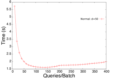
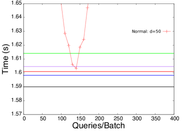
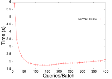
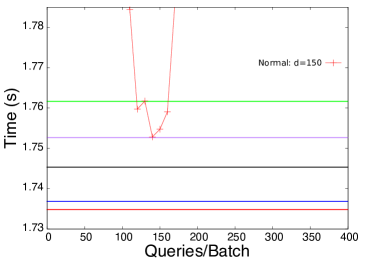
Figure 9: Response time vs. queries/batch ($s$) for the periodic query batch method for S5 (a) and S6 (c) (RandWalk-Normal dataset). Panels (b) and (d) correspond to zoomed in versions of (a) and (c) respectively, to highlight the minimum response times. The colored lines correspond to the same algorithms as shown in Figure 7.

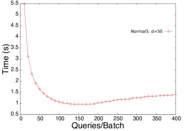
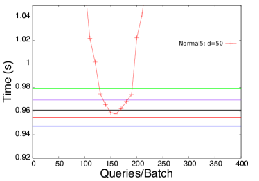
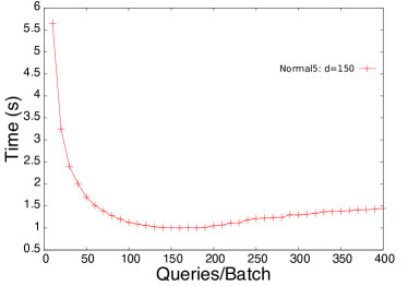
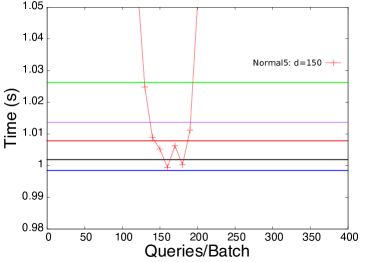
Figure 10: Response time vs. queries/batch ($s$) for the periodic query batch method for S7 (a) and S8 (c) (RandWalk-Normal5 dataset). Panels (b) and (d) correspond to zoomed in versions of (a) and (c) respectively, to highlight the minimum response times. The colored lines correspond to the same algorithms as shown in Figure 7.

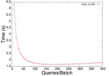
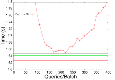
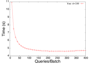
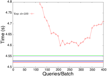
Figure 11: Response time vs. queries/batch ($s$) for the periodic query batch method for S9 (a) and S10 (c) (RandWalk-Exp dataset). Panels (b) and (d) correspond to zoomed in versions of (a) and (c) respectively, to highlight the minimum response times. The colored lines correspond to the same algorithms as shown in Figure 7.

We now evaluate the relative merit of the algorithms for creating query segment batches (Periodic, SetSplit, GreedySetSplit). Response time results for experimental scenarios S1 to S10 are shown in these figures: Figure 7 (for S1 and S2), Figure 8 (for S3 and S4), Figure 9 (for S5 and S6), Figure 10 (for S7 and S8), and Figure 11 (for S9 and S10). For each experimental scenario, the response time of the Periodic algorithm is plotted versus the batch size on the left-hand side of the figure. A zoomed-in version of each plot is shown on the right-hand side, which shows the neighborhood of the best batch size for Periodic, as well as the response times of the SetSplit and GreedySetSplit algorithms (which are shown as horizontal lines). These results correspond to a “best case” for the SetSplit and GreedySetSplit algorithms, for two reasons. First, the response time results do not include the time necessary to compute the query batches. This time is negligible for Periodic, but can be significant for SetSplit and even for GreedySetSplit, as discussed at the end of this section. Second, using an exhaustive search, for each experimental scenario we have determined the best parameter configuration for the SetSplit and GreedySetSplit algorithms (i.e., the best number of batches for SetSplit-Fixed, the best maximum batch size for SetSplit-Max, the best minimum and maximum batch size for SetSplit-MinMax, the best minimum batch size for GreedySetSplit-Min, and the best maximum batch size for GreedySetSplit-Max). The results in Figures 7-11 are summarized in Table 2, which shows for each algorithm, and each experimental scenario, the percentage response time difference relative to the response time of the best algorithm for that experimental scenario. We show two versions of the Periodic algorithm. PeriodicBest corresponds to Periodic when using the batch size that leads to the lowest response time for the experimental scenario at hand. PeriodicGood corresponds to Periodic but using the worst batch size in a -20/+20 neighborhood of the best batch size (i.e., the batch size in that interval that leads to the highest response time).

Table 2: Percentage response time difference relative to the lowest response time for all algorithms and experimental scenarios. Results for the algorithm with the lowest response time shown in boldface.

Algorithm	S1	S2	S3	S4	S5	S6	S7	S8	S9	S10
GreedySetSplit-Max	0.15	0.15	0.15	0.00	0.00	0.60	1.44	0.34	1.29	0.16
GreedySetSplit-Min	0.00	0.24	0.00	0.15	0.52	0.11	0.00	0.00	0.93	0.10
SetSplit-Fixed	1.11	1.69	1.03	1.02	0.92	1.03	2.34	1.52	562.90	0.62
SetSplit-Max	1.50	1.97	1.02	0.35	1.51	1.54	3.37	2.78	0.90	0.69
SetSplit-MinMax	0.24	0.33	0.10	0.17	0.69	0.00	0.77	0.93	0.00	0.00
PeriodicBest	0.37	0.00	0.23	0.50	0.83	1.03	1.11	0.09	1.50	1.69
PeriodicGood	3.21	2.47	1.64	3.56	2.15	1.43	2.21	1.05	2.52	2.69

Some trends are clearly seen in the results. Over the 10 experimental scenarios, the SetSplit and GreedySetSplit algorithms all lead to response times that are close to each other (within 3.4%). One exception is for SetSplit-Fixed, which leads to a significantly larger response time for S9 (about a factor 10 larger than the other algorithms). Recall that SetSplit-Fixed creates a fixed number of batches without any constraint on the maximum batch size. S9 contains entries with exponentially distributed temporal extents, which causes SetSplit-Fixed to create a few very large batches at the tail of the distribution (which leads to the smallest minDiff value - line 8 in Algorithm 2). These large batches are the reason for the high response time of SetSplit-Fixed. This problem does not occur for experimental scenario S10 due to the larger total number of query segments. An interesting finding is that the GreedySetSplit algorithms, even though they use a single pass through the query segments, do well. GreedySetSplit-Max, resp. GreedySetSplit-Min, leads to the lowest response time in 2, resp. 4, of the 10 experimental scenarios. Overall, the GreedySetSplit algorithms are among the 3 best algorithms for each experimental scenario. This suggests that the quadratic complexity of the SetSplit algorithm to attempt a less local optimization is in fact unnecessary.

The key observation from our results is that Periodic leads to good performance. As seen in Figure 7, the response time of Periodic can be high for some batch sizes. However, when using the best batch size, Periodic can produce response time on par or even better than that of the GreedySetSplit and SetSplit algorithms. Overall, for each experimental scenario PeriodicBest leads to response times at most 1.69% larger than that of the best GreedySetSplit or SetSplit algorithm for that scenario. It even leads to the lowest response time for experimental scenario S2. Even when Periodic does not use the best batch size it leads to good results. PeriodicGood still leads to response times at most 3.56% larger than the best GreedySetSplit or SetSplit algorithm over the 10 experimental scenarios.

As explained above, our results do not include the time to compute the batches. Due to quadratic complexity, for the SetSplit algorithms this time is large, factors larger than the query response time for our experimental scenarios. Overall, when adding the time to compute the batches (on the CPU), we find that the SetSplit algorithms lead to average response time more than 4.69 times larger than PeriodicBest and up to 8.84 times larger (discounting SetSplit-Fixed for experimental scenario S9, which leads to response time 12.76 times larger). The GreedySetSplit algorithms fare better when compared to PeriodicBest, with response times only up to 2.9% larger over all experimental scenarios. This is because these algorithms have linear complexity.

We conclude that although computing batches that reduce wasteful interactions, as in the SetSplit and GreedySetSplit algorithms, is an appealing idea, in practice it does not outperform a simple periodic approach. This is because the small response time benefit due to the use of better batches is offset by the CPU time overhead of computing these batches. One drawback of Periodic is that one must specify a good batch size, i.e., a batch size in a neighborhood of the best batch size. In the next section, we propose performance modeling techniques that can be used to determine such a good batch size.

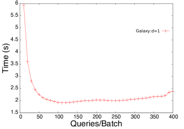
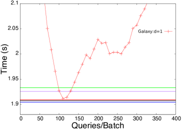
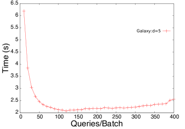
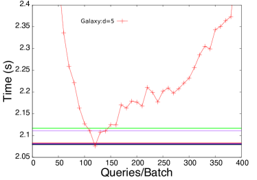
Figure 7: Response time vs. queries/batch ($s$) for the periodic query batch method for S1 (a) and S2 (c) (Galaxy dataset). Panels (b) and (d) correspond to zoomed in versions of (a) and (c) respectively, to highlight the minimum response times. The colored lines correspond to the best response time from the query splitting algorithms, where SetSplit-Fixed is purple, SetSplit-Max is green, SetSplit-MinMax is red, GreedySetSplit-Min is blue, and GreedySetSplit-Max is black.

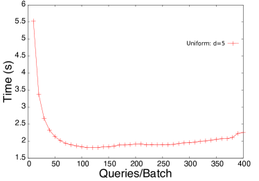
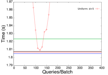
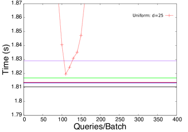
Figure 8: Response time vs. queries/batch ($s$) for the periodic query batch method for S3 (a) and S4 (c) (RandWalk-Uniform dataset). Panels (b) and (d) correspond to zoomed in versions of (a) and (c) respectively, to highlight the minimum response times. The colored lines correspond to the same algorithms as shown in Figure 7.

8 Performance Modeling

Most previous works on spatiotemporal database querying, and in particular works that consider distance threshold queries [3, 11, 12], rely on index-trees, such as R-trees. These index-trees have complex performance behavior as the traversal time depends on the set of pointers followed on a path toward a leaf node, which is highly data dependent. As a result, predicting query response time is challenging. An added difficulty in the case of distance threshold queries is that one query may lead to a large result set while another may lead to an empty result set.

Because designed for GPU execution, the indexing scheme proposed in this work (Sections 4 and 5) does not rely on index-trees. While not completely free of data-dependent behavior, the more deterministic behavior of this scheme makes it possible to predict query response time. And in particular, such prediction is sufficiently accurate to determine a good batch size for the Periodic algorithm.

The model consists of a GPU component and CPU component. The GPU component accounts for the invocation overhead and execution time of each individual kernel invocation, so that summing over all invocations gives the estimated GPU time for processing the entire set of query segments. The CPU component accounts for the time to perform memory allocations, set kernel parameters, send query data to the GPU, receive result sets from the GPU, marshal data, and perform other CPU-side computations (e.g., counter and pointer updates). Figure 12 shows response time results for the S1 experimental scenario, showing both the CPU and GPU components. The GPU curve shows an initial decrease as the batch size, $s$, increases in the interval $10\leq s\leq 40$. This decrease is because for low $s$ values the GPU device is underutilized and the kernel invocation overhead is large due to many such invocations. For $s\geq 50$, the GPU time increases due to the increasing number of interactions that must be computed (as explained in Section 6). The CPU time curve shows a steady decrease as $s$ increases. This is because the smaller the value of $s$ the more kernel invocations and thus the more work done on the CPU. We show two portions of the CPU time. The time necessary to perform kernel invocations, including the transfer of query segments from the CPU to the GPU, is shown as a shaded cyan portion below the CPU curve. The shaded blue portion corresponds to the time necessary for transferring result sets from the GPU back to the CPU.

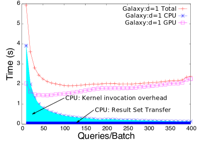
Figure 12: Response time vs. queries/batch ($s$) for S1 (Galaxy dataset with $d=1$). The individual CPU and GPU components are shown.

8.1 GPU Component

8.1.1 Model

In this section, we derive an empirical model for the GPU component of our performance model. Let us use $T^{GPU}(i,c)$ to denote the GPU time for a kernel invocation that computes the $i$ interactions necessary for comparing a batch of $i/c$ query segments against $c$ candidate segments (using $c$ GPU threads). Let us use $\Theta^{GPU}(i,c)$ to denote the overhead of launching a no-op kernel for $q$ query segments and $i$ interactions (the overhead depends both on the number of queries and on the number of GPU threads). Given the $i$ interactions to be computed, we denote by $\alpha$ the fraction of these interactions that lead to an item being added to the result set (i.e., both a temporal hit and a spatial hit), by $\beta$ the fraction of these interactions for which the entry segment does not overlap the query segment temporally (i.e., a temporal miss), and by $\gamma$ the fraction of these interactions for which the entry segment overlaps the query segment temporally but not spatially (i.e., a temporal hit but a spatial miss). We have $\alpha+\beta+\gamma=1$. We distinguish these three cases because the computational cost is different in each. Candidate segments that are temporal misses can be determined with only a few instructions (i.e., comparing temporal extremities of query and candidate segments). Candidate segments that are temporal hits but spatial misses require more instructions (i.e., spatial extremities comparisons). Candidate segments that should be added to the result set require even more instructions to be performed (i.e., determining the actual overlapping temporal interval). One can view the computation of an interaction as a set of comparisons and moving distance calculations, but these comparisons and computations are short-circuited whenever a segment is found to be a temporal or spatial miss.

We denote by $T_{1}(i,c)$, $T_{2}(i,c)$, and $T_{3}(i,c)$ the time for a kernel invocation with $i$ interactions so that all $c$ candidate segments are temporal and spatial hits, temporal misses, and temporal hits and spatial misses, respectively. This leads us to the following model:

$$T^{GPU}(i,c)=T^{GPU}_{1}(\alpha i,c)+T^{GPU}_{2}(\beta i,c)+T^{GPU}_{3}(\gamma i,c)-2\Theta^{GPU}(i,c).$$

The first three terms above each include a $\Theta^{GPU}(i,c)$ component, hence the subtracted fourth term. $T_{GPU}(i,c)$ is computed for each batch, and the sum gives the total GPU time assuming the batch size is $s$:

$$T^{GPU}(s)=\sum_{j=0}^{|Q|/s}T^{GPU}(i_{j},i_{j}/s).$$

$Q$ is the total set of query segments (for simplicity this equation assumes that $s$ divides $|Q|$). $i_{j}$ is the number of interactions that must be computed for the $j$-th query batch, which is determined based on the entry segment bins (see Section 4). Therefore $i_{j}/s$ is the number of candidate entry segments for the $s$ query segments in the batch.

In this model, parameters $\alpha$, $\beta$ and $\gamma$ depend on the dataset and the query. They must thus be determined empirically for typical scenarios. By contrast, the functions $\Theta^{GPU}$, $T^{GPU}_{1}$, $T^{GPU}_{2}$, $T^{GPU}_{3}$ depend only the hardware characteristics of the platform. In what follows we describe how we estimate these parameters. Note that this estimation is done for each batch of $s$ queries.

8.1.2 Estimating $\alpha$, $\beta$ and $\gamma$

Recall that $\alpha$ is, for a kernel invocation on a query batch, the fraction of interactions that lead to a new item being added to the result set. Given that it is dataset dependent, we use a pragmatic approach to estimate $\alpha$ for a particular dataset once and for all, i.e., before the dataset is being queried in “production” use. Depending on the temporal distribution of the entry segments, there may be time periods with few active trajectories and some with many, resulting in a non-uniform distribution of query hits throughout time. To estimate $\alpha$, we divide the dataset into $numEpochs$ temporal epochs. For each epoch we select a batch of $s$ sample queries that fall within the epoch. We do this by randomly selecting $s$ consecutive query segments from a representative query dataset. We then execute our kernel and calculate the fraction of interactions that produced result items. We perform this over enough trials such that the predicted total number of result set items is within 5% of the total true number of result set items. This procedure yields an $\alpha$ estimate for each epoch. This estimate may be inaccurate if the sample queries are not representative of queries that will be processed in production. Also, if too low a value of $numEpochs$ is used, then the $\alpha$ estimates are more likely to be inaccurate since transient temporal patterns are then averaged over larger epochs. Using $numEpochs=1$ is a degenerate case in which our model would assume that for any kernel invocation the query hit probability is the same. This may be accurate for a temporally uniform dataset, but vastly inaccurate for datasets that exhibit temporal transience. In all the experiments presented hereafter we use $numEpochs=50$.

Unlike $\alpha$, $\beta$ can be computed precisely. For a given set of $s$ query segments, one can determine which entry segments they may temporally overlap using the bins in our indexing scheme (see Section 4). Then, with two nested loops one can simply compare the temporal extremities of each query segment to that of each entry segment, yielding an exact value for $\beta$. Parameter $\gamma$ is computed as $1-\alpha-\beta$.

To summarize, for a given dataset we compute once and for all a set of $\alpha$ estimates for each epoch and for the full range of (reasonable) $s$ values. Then, for each batch of $s$ queries we compute an $\alpha$ estimate, $\beta$ and $\gamma$. Therefore, for each candidate $s$ value we can plug appropriate values of these three parameters into the $T^{GPU}$ performance model.

8.1.3 Estimating $T^{GPU}_{1}$, $T^{GPU}_{2}$, $T^{GPU}_{3}$ and $\Theta^{GPU}$

The $T^{GPU}_{1}$, $T^{GPU}_{2}$, $T^{GPU}_{3}$ and $\Theta^{GPU}$ functions depend only on the implementation of the kernel and the hardware characteristics of the platform. As a result, we can empirically estimate these time components based on benchmark results. Let us consider $T^{GPU}_{1}$, i.e., the kernel response time when all interactions are both temporal hits and spatial hits. The same approach is used to estimate $T^{GPU}_{2}(i,c)$, $T^{GPU}_{3}(i,c)$ and $\Theta^{GPU}(i,c)$.

We generate a synthetic dataset and query set in which all interactions are guaranteed to be both temporal and spatial hits. Figure 13 shows a subset of our benchmark results as response time vs. number of interactions for various numbers of candidate entry segments, as measured on our target platform. Given a number of interactions, $i$, and a number of candidate entries, $c$, we simply use linear interpolation to determine a response time prediction $T^{GPU}_{1}(i,c)$ from the benchmark results.

Figure 13: Interactions vs. response time for a selection of entries. The data shown corresponds to a range of 1-300 benchmarked queries.

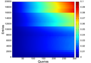
(a) 1-300 queries

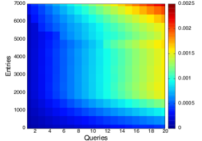
(b) 1-20 queries

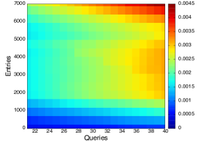
(c) 21-40 queries

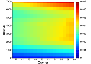
(d) 41-60 queries

Figure 14: Benchmark of interactions that all are within the query distance. Panel (a) shows a large selection of the data, across a range of 300 queries, and (b), (c) and (d) show detailed versions of the data between 1-60 queries.

Figure 14 (a) shows a broader range of benchmark results, shown as heat maps of the response time vs. the number of candidate entries, $c$ and the number of queries $q=i/c$. In Figure 14 (a) we observe that there are discontinuities in response time. We attribute these discontinuities mainly to thread scheduling factors on the GPU. Regardless, they will be a source of modeling error due to our use of linear interpolation. Figure 14 (b), (c), and (d) show plots with queries in the range of 1 to 60. We see somewhat smoother response time trends, particularly in Figure 14 (c) and (d) suggesting that in that range the use of linear interpolation should lead to less error. Since we know that the batch size, and thus the number of candidate segments, should be relatively small, then one may expect that modeling error due to linear interpolation could also be small.

The above modeling approach assumes that the kernel response time can be estimated from the benchmark-based models of $T^{GPU}_{1}$, $T^{GPU}_{2}$, $T^{GPU}_{3}$, executed separately. However, an actual kernel execution consists of a mix of temporal and spatial hits, temporal misses, and temporal hits but spatial misses. One may thus wonder whether the notion of separating the model into three components can lead to reasonable response time predictions. To answer this question we compared executions of the three benchmark kernels to a mixed execution, using various synthetic datasets and query sets with $\alpha=\beta=\gamma=1/3$.

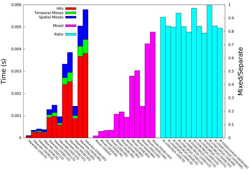
Figure 15: GPU response time vs. test cases of mixed and separated kernel invocations.

Figure 15 shows the response time vs. test case, where the first two histograms correspond to the separate and mixed tests, respectively, and the rightmost histogram shows the ratio of mixed to separate response times. The test cases are identified as “Separate” or “Mixed”, followed by the number of entry segments and the batch size. Since $\alpha=\beta=\gamma=1/3$, then the number of queries of each type ($\alpha$, $\beta$, $\gamma$) is equal to the total number of queries in an experimental scenario divided by 3. For example, consider the scenario where there are 9 queries in total, Separate-100E/3Q (3 queries of each type) is compared to Mixed-100E/9Q, where we compare three kernel executions with queries of type $\alpha$, $\beta$, and $\gamma$ each with a query batch size of 3, to one kernel execution with 9 queries, which are a mixture of query types $\alpha$, $\beta$, and $\gamma$. To allow for fair comparisons we have discounted the kernel invocation overhead from all results (this overhead occurs three times in the Separate results but only once in the Mixed results).

The first observation is that the Mixed executions have lower response times than the Separate counterparts. This may seem counter-intuitive because the Mixed executions, unlike the Separate executions, should have a high degree of branch divergence, thus causing partially serialized thread executions on the GPU [15]. However, in Mixed executions the entry segments are retrieved from the GPU’s global memory and stored into private memory once, and are then reused. This does not occur in the Separate executions as entry segments have to be reloaded from global memory into private memory at each kernel invocation. Regardless, the rightmost histogram in Figure 15 shows that the error due to using Separate executions is relatively consistent and in the 1%-20% range. As a result, we expect that our modeling approach should lead to reasonable response time predictions. Furthermore, since the error is consistent, the same bias should apply when comparing the estimated response time for various candidate batch sizes.

8.2 CPU Component

To model the CPU time, we propose an empirical model for each of the two portions of the CPU time shown in Figure 12 as shaded cyan and blue areas. These models consist of simple curve fitting based on benchmark results ($R^{2}$ values for the fits are above 0.9999).

To estimate $T^{CPU}_{1}(s)$, the portion of the CPU time that corresponds to the kernel invocation overhead for a batch size $s$ (the cyan area in Figure 12), we generate a synthetic dataset with $\alpha\approx 0$. With a very low value of $\alpha$, the result set has negligible size. As a result, kernel response time is approximately equal to the aggregate kernel invocation overhead. We thus obtain a kernel invocation overhead curve for the full range of possible batch sizes. This benchmark must be executed for various total numbers of query segments so that for a query set $Q$, our model uses benchmark results obtained for approximately $|Q|$ query segments. In practice, one would thus run the benchmark for various numbers of query segments, obtaining a family of CPU response time curves. In all experiments hereafter, $|Q|$=40,000, and we thus use 40,000 queries as well in our benchmark. We obtain the following response time fitted curve:

$$T^{CPU}_{1}(s)=-0.0017+32.2946\times s^{-0.9528}.$$ (1)

To estimate $T^{CPU}_{2}$, the portion of the CPU time that corresponds to the transfer of the result set from the GPU to the CPU (the blue area in Figure 12), we rely on the $\alpha$ parameter defined in the GPU component of our performance model and estimated as described in Section 8.1.2. Using $\alpha$, we can determine the number of result set items generated by each kernel invocation. Summing over all kernel invocations and multiplying by the size in bytes of a result set item yields the total size of the result set, which we denote by $\sigma$. Assuming that $T^{CPU}_{2}$ does not depend on $s$, we can then estimate it by dividing $\sigma$ by the GPU-CPU bandwidth measured on the platform. On our target platform the model is as follows:

$$T^{CPU}_{2}(\sigma)=1.54\times 10^{-8}\times\sigma.$$ (2)

In the end, the total CPU time is modeled as: $T^{CPU}(s,\sigma)=T^{CPU}_{1}(s)+T^{CPU}_{2}(\sigma)$, and the total response time is modeled as $T^{CPU}(s)+T^{GPU}(s,\sigma)$.

8.3 Model Evaluation

Figure 16 shows actual and modeled response times vs. the batch size for a selection of our experimental scenarios. The CPU and GPU model components are shown with separate curves. The general trends of the actual response time are respected by the model. In some instances, the model tracks the actual response time well, while on other it exhibits some deviations. However, the main purpose of our model is not to predict response time perfectly, but to produce a sufficiently coherent prediction so that a good batch size can be selected. Figure 16 (b) presents the model for the Galaxy dataset with $d=5$. The model suggests that $s=80$ yields the best response time; however, the actual best response time occurs when $s=120$. Had $s=80$ been chosen, $s=120$ would be 6.3% faster. Such results are summarized in Table 3 for our 10 experimental scenarios, where the Model column gives the batch size based on the model, the Actual column gives the empirically best batch size, and the Slowdown column gives the response time slowdown due to using the model-driven batch size, as a percentage. Note that S3 has few elements in its result set, and thus has a low value of $\alpha$ across all epochs. For this scenario, it was not possible to assure that the total estimated number of result set items is within 5% of the actual number across all values of $s$.

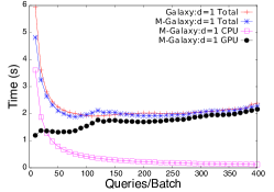
(a) S1: Galaxy.

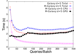
(b) S2: Galaxy.

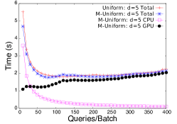
(c) S3: RandWalk-Uniform.

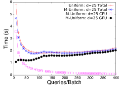
(d) S4: RandWalk-Uniform.

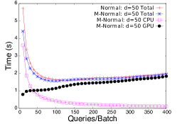
(e) S5: RandWalk-Normal.

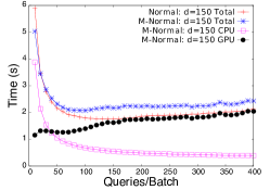
(f) S6: RandWalk-Normal.

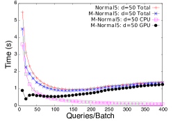
(g) S7: RandWalk-Normal5.

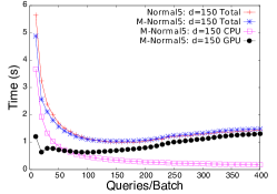
(h) S8: RandWalk-Normal5.

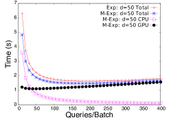
(i) S9: RandWalk-Exp.

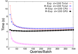
(j) S10: RandWalk-Exp.

Figure 16: Modeled response times vs. queries per batch ($s$) for searches on each dataset. The red curve shows the actual response time, the blue curve shows the modeled total response time, where the CPU (magenta) and GPU (black) model components added together equal the modeled total (blue) curve.

Table 3: Model Results.

Search	Model	Actual	Slowdown
S1	80	110	4.8%
S2	80	120	6.3%
S3	80	120	4.5%
S4	80	110	4.5%
S5	100	140	2.8%
S6	100	140	2.3%
S7	140	160	0.8%
S8	150	160	0.58%
S9	170	220	0.1%
S10	200	210	0.97%

In these results we find that the worst slowdown is less than 7% and that in many cases the slowdown is negligible. We conclude that, in spite of data dependency challenges, our model is useful for determining a good batch size to use with the Periodic algorithm and for predicting the total query response time. An interesting question is whether our modeling approach can be used for response time prediction purposes for other spatiotemporal queries.

9 Conclusions

In this work, we have studied the efficient execution of an in-memory trajectory similarity search, the distance threshold search, on the GPU. The objective is to minimize response time in an online setting in which a series of kernel invocations are performed to process a potentially large query set. We have shown that the parallelism afforded by the GPU, provided a GPU-friendly indexing method is used, can outperform multithreaded CPU implementations that use an in-memory R-tree index. We have proposed such a GPU-friendly indexing method. While conceptually simple, this method may be suitable for indexing spatial and spatiotemporal objects for parallel architectures in general, as described in [26]. We have proposed several algorithms for partitioning a query set into individual batches, so as to reduce memory pressure and computational cost on the GPU. We have found that, when considering the cost to compute the batches, a simple algorithm that partitions the query set into fixed-size batches leads to competitive response times.

Modeling the performance of algorithms that process moving objects is a challenge due to the spatiotemporal nature of data. Furthermore, in the context of spatiotemporal databases, where index-trees are paramount, the non-deterministic nature of tree traversals adds an additional source of performance uncertainty. The indexing method proposed in this work obviates some of this data-dependent uncertainty. As a result, we are able to derive a reasonably accurate response time model. This model, which considers both CPU and GPU time, is sufficient for predicting a good batch size for a given dataset. Furthermore, in some instances, the model is adequate to estimate the actual query response time across a range of query batch sizes. This result is encouraging, as it suggests that predicting query response time on the GPU, at least with some indexing techniques, is feasible, making it possible to assess the tractability of spatiotemporal queries across a range of application domains. In particular, such query response time prediction will be crucial for for estimating the compute time for the astrophysical application that is the initial motivation for this work. Future work directions include utilizing multiple work queues to overlap computation with communication between host and device, investigating other GPU-friendly indexes and applying our performance model to other spatiotemporal queries.

References

- [1] http://navet.ics.hawaii.edu/%7Emike/datasets/GPU/trajdat.zip. Accessed 25-May-2014.
- [2] Combining cpu and gpu architectures for fast similarity search. Distributed and Parallel Databases, 30(3–4):179–207, 2012.
- [3] S. Arumugam and C. Jermaine. Closest-point-of-approach join for moving object histories. In Proc. of the 22nd Intl. Conf. on Data Engineering, pages 86–95, 2006.
- [4] V. P. Chakka, A. Everspaugh, and J. M. Patel. Indexing large trajectory data sets with seti. In Proc. of the Conf. on Innovative Data Sys. Research, pages 164–175, 2003.
- [5] P. Cudre-Mauroux, E. Wu, and S. Madden. TrajStore: An Adaptive Storage System for Very Large Trajectory Data Sets. In Proc. of the 26th Intl. Conf. on Data Engineering, pages 109–120, 2010.
- [6] E. Frentzos, K. Gratsias, N. Pelekis, and Y. Theodoridis. Algorithms for Nearest Neighbor Search on Moving Object Trajectories. Geoinformatica, 11(2):159–193, 2007.
- [7] Luca Forlizzi, Ralf Hartmut Güting, Enrico Nardelli, and Markus Schneider. A data model and data structures for moving objects databases. In Proc. of ACM SIGMOD Intl. Conf. on Management of Data, pages 319–330, 2000.
- [8] Elias Frentzos, Kostas Gratsias, Nikos Pelekis, and Yannis Theodoridis. Nearest neighbor search on moving object trajectories. In Proc. of the 9th Intl. Conf. on Advances in Spatial and Temporal Databases, pages 328–345, 2005.
- [9] Yun-Jun Gao, Chun Li, Gen-Cai Chen, Ling Chen, Xian-Ta Jiang, and Chun Chen. Efficient k-nearest-neighbor search algorthims for historical moving object trajectories. J. Comput. Sci. Technol., 22(2):232–244, 2007.
- [10] M. G. Gowanlock, D. R. Patton, and S. M. McConnell. A Model of Habitability Within the Milky Way Galaxy. Astrobiology, 11:855–873, 2011.
- [11] Michael Gowanlock and Henri Casanova. In-Memory Distance Threshold Queries on Moving Object Trajectories. In Proc. of the Sixth Intl. Conf. on Advances in Databases, Knowledge, and Data Applications, pages 41–50, 2014.
- [12] Michael Gowanlock, Henri Casanova, and David Schanzenbach. Parallel In-Memory Distance Threshold Queries on Trajectory Databases. In Proc. of the Sixth Intl. Conf. on Advances in Databases, Knowledge, and Data Applications, pages 80–83, 2014.
- [13] Ralf Hartmut Güting, Thomas Behr, and Jianqiu Xu. Efficient k-nearest neighbor search on moving object trajectories. The VLDB Journal, 19(5):687–714, 2010.
- [14] Antonin Guttman. R-trees: a dynamic index structure for spatial searching. In Proc. of ACM SIGMOD Intl. Conf. on Management of Data, pages 47–57, 1984.
- [15] Tianyi David Han and Tarek S. Abdelrahman. Reducing branch divergence in gpu programs. In Proc. of the 4th Workshop on General Purpose Processing on Graphics Processing Units, pages 3:1–3:8, 2011.
- [16] Hoyoung Jeung, Man Lung Yiu, Xiaofang Zhou, Christian S. Jensen, and Heng Tao Shen. Discovery of convoys in trajectory databases. Proc. VLDB Endow., 1(1):1068–1080, August 2008.
- [17] Kimikazu Kato and Tikara Hosino. Multi-gpu algorithm for k-nearest neighbor problem. Concurrency and Computation: Practice and Experience, 24(1):45–53, 2012.
- [18] Zhenhui Li, Ming Ji, Jae-Gil Lee, Lu-An Tang, Yintao Yu, Jiawei Han, and Roland Kays. Movemine: Mining moving object databases. In Proc. of the 2010 ACM SIGMOD Intl. Conf. on Management of Data, pages 1203–1206, 2010.
- [19] Lijuan Luo, M. D F Wong, and L. Leong. Parallel implementation of r-trees on the gpu. In Design Automation Conf. (ASP-DAC), 2012 17th Asia and South Pacific, pages 353–358, Jan 2012.
- [20] Jia Pan and Dinesh Manocha. Fast gpu-based locality sensitive hashing for k-nearest neighbor computation. In Proc. of the 19th ACM SIGSPATIAL Intl. Conf. on Advances in Geographic Information Systems, pages 211–220, 2011.
- [21] Dieter Pfoser, Christian S. Jensen, and Yannis Theodoridis. Novel Approaches in Query Proc. for Moving Object Trajectories. In Proc. of the 26th Intl. Conf. on Very Large Data Bases, pages 395–406, 2000.
- [22] Y. Theodoridis, M. Vazirgiannis, and T. Sellis. Spatio-Temporal Indexing for Large Multimedia Applications. In Proc. of the Intl. Conf. on Multimedia Computing and Systems, pages 441–448, 1996.
- [23] Marcos R. Vieira, Petko Bakalov, and Vassilis J. Tsotras. On-line discovery of flock patterns in spatio-temporal data. In Proc. of the 17th ACM SIGSPATIAL Intl. Conf. on Advances in Geographic Information Systems, pages 286–295, 2009.
- [24] Simin You, Jianting Zhang, and Le Gruenwald. Parallel spatial query processing on gpus using r-trees. In Proc. of the 2nd ACM SIGSPATIAL Intl. Workshop on Analytics for Big Geospatial Data, BigSpatial ’13, pages 23–31, New York, NY, USA, 2013. ACM.
- [25] Jianting Zhang, Simin You, and Le Gruenwald. U2STRA: High-performance Data Management of Ubiquitous Urban Sensing Trajectories on GPGPUs. In Proc. of the 2012 ACM Workshop on City Data Management Workshop, CDMW ’12, pages 5–12, 2012.
- [26] Jianting Zhang, Simin You, and Le Gruenwald. Parallel online spatial and temporal aggregations on multi-core CPUs and many-core GPUs. To Appear in Information Systems, pages –, 2014.