Does the Period of a Pulsating Star Depend on its Amplitude?

John R. Percy and Jeong Yeon (JY) Yook
Department of Astronomy and Astrophysics
University of Toronto
Toronto ON
Canada M5S 3H4

Abstract Several classes of pulsating stars are now known to undergo slow changes in amplitude; these include pulsating red giants and supergiants, and yellow supergiants. We have used visual observations from the AAVSO International Database, and wavelet analysis of 39 red giants, 7 red supergiants, and 3 yellow supergiants, to test the hypothesis that an increase in amplitude would result in an increase in period, because of non-linear effects in the pulsation. For most of the stars, the results are complex and/or indeterminate, due to the limitations of the data, the small amplitude or amplitude variation, or other processes such as random cycle-to-cycle period fluctuations. For the dozen stars which have substantial amplitude variation, and reasonably simple behavior, there is a 75-80% tendency to show a positive correlation between amplitude and period.

1. Introduction

Galileo Galilei is noted for (among other things) observing that the period of the swing of a pendulum does not depend on the amplitude of the swing. For most vibrating objects, however, there are non-linear effects which cause the period to increase slightly if the amplitude becomes sufficiently large.

We have recently noted that there are systematic, long-term variations in amplitude in pulsating red giants (Percy and Abachi 2013), pulsating red supergiants (Percy and Khatu 2014), and pulsating yellow supergiants (Percy and Kim 2014). The purpose of this project was to investigate whether there might be systematic changes in period which accompany the changes in amplitude. This possibility has already been suggested as occuring in R Aql, BH Cru, and S Ori (Bedding et al. 2000, Zijlstra et al. 2004).

Our study is complicated by several factors. Stars undergo small, slow evolutionary changes in period. They also undergo random cycle-to-cycle fluctuations in period (Eddington and Plakidis 1929, Percy and Colivas 1999). We have shown that, for some reason, the amplitudes themselves are variable. The stars are complicated: red giants and supergiants have large, convective hot and cool regions on their surfaces. Furthermore, the stars rotate with periods which are comparable with the time scales for amplitude change. For these reasons, it may be difficult to isolate any non-linear effect of changing amplitude on period.

2. Data and Analysis

We used visual observations, from the AAVSO International Database, of the stars listed in Tables 1-3. See ”Notes on Individual Stars” for remarks on some of these. Percy and Abachi (2013) discussed some of the limitations of visual data which must be kept in mind when analyzing the observations, and interpreting the results, but only visual observations are sufficiently dense, sustained, and systematic for use in this project. The data, extending from JD(1) to JD(1) + $\Delta$JD [JD = Julian Date, in days] as given in the tables, were analyzed using the VSTAR package (Benn 2013; www.aavso.org/vstar-overview), especially the wavelet (WWZ) analysis routine. The periods of the stars had previously been determined with the DCDFT routine. For the wavelet analysis, as in our previous papers, the default values were used for the decay time c (0.001) and time division $\Delta$t (50 days). The results are sensitive to the former, but not to the latter.

We generated light curves and graphs of period and amplitude versus JD, but our main tool for analysis was graphs of amplitude versus period, as shown in the figures. For each of these, the method of least squares was used to determine the straight line of best fit, the slope k of this fit, the standard error $\sigma$ of the fit, and the coefficient of correlation R. Tables 1-3 give the star, period in days, initial JD and range of JD, amplitude and amplitude range in magnitudes, k, $\sigma$, k/$\sigma$, R, and any notes. See also the “Notes on Individual Stars”. In the last column, an asterisk (*) indicates that k/$\sigma$ is greater than 3, and a double asterisk (**) indicates that R $\geq$ 0.5 i.e. the results are statistically significant. The notation e-x means 10 to the power x. The Notes column also includes a qualitative description of the shape and trajectory of the semi-amplitude versus period plots: 1 indicates positive slope, 2 indicates negative slope, 3 indicates non-linear, 4 indicates vertical lines, 5 indicates counterclockwise, 6 indicates clockwise, 7 indicates irregular trajectory, and 8 indicates a sinusoidal trajectory. The spectral types in the figure captions are from SIMBAD.

3. Results

3.1. Red giants

Table 1 shows the results of the single-mode variables from Kiss et al. (2006), Percy and Abachi (2013), Bedding et al. (2000), and Zijlstra et al. (2004). In total, 39 pulsating red giants are listed on the table and 26 of them have a positive k and 13 of them have a negative k.

Figure 1 shows the semi-amplitude versus period relationship for BH Cru. It displays a strong, positive correlation between semi-amplitude and period; and there is almost no non-linearity. The relation is also clear from the plots of period-JD and amplitude-JD (Bedding et al. (2000). Note that we are using about 14 more years of data than Bedding et al. (2000).

Figure 2 shows the semi-amplitude versus period plot for R Aql. There is a strong, positive correlation between them as listed in Table 1. This agrees with the discussion of Bedding et al. (2000) that R Aql shows some relationship between period and amplitude. However, there is local non-linearity in addition to the linear correlation, which suggests that there is also some other process which affects the period. The individual period and amplitude plots show that, whereas the period is decreasing monotonically from 310 to 270 days, the amplitude is decreasing but also undergoing fluctuations, perhaps due to stochastic excitation and decay.

Figure 3 is a semi-amplitude versus period plot for S Ori, which is again from Bedding et al. (2000). This one also has a positive correlation; however, there is a global non-linearity and the linear fit does not represent the relationship between amplitude and period very well. In this case, the individual period and amplitude plots show that the period is undergoing fluctuations between 405 and 440 days.

Figure 4 is for GY Aql, a pulsating red giant from Percy and Abachi (2013). The semi-amplitude and the period of GY Aql have a sinusoidal relationship and the linear fit is not a good representation of the data. This plot is non-linear; however, this sinusoidal pattern shows more regularity than other non-linear plots. Note, however, that the change in amplitude is small, both absolutely and as a fraction of the average amplitude.

Figure 5 is for S Aur from Percy and Abachi (2013). There is a positive correlation between the semi-amplitude and period, but this obviously not the dominant process affecting the period.

Figure 6 shows the semi-amplitude versus period for S Cam. There is a positive correlation with some non-linearity. The change in amplitude is relatively small.

Figure 7 is for DM Cep and it has a negative slope with some non-linearity. The data has a gap in the mid-region of the data, and the amplitude is very small.

Figure 8 is for SY Per and there is a positive correlation. There is a local non-linearity in the plot; however, the line of the best fit is a good representation of the data globally.

Figure 9 is for UZ Per. UZ Per has a long period and a small change in amplitude, so the negative slope is not really meaningful.

Figure 10 is for W Tau. There is a positive correlation between semi-amplitude and period, with some non-linearity in the plot in addition to the global linear trend.

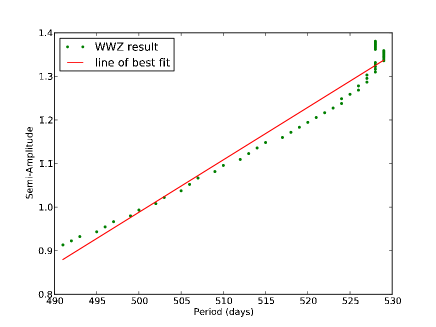
Figure 1: Amplitude versus period for BH Cru (SC4.5-7/8e). The correlation is excellent, as was apparent from the graphs of period and amplitude versus JD (Bedding et al. 2000)

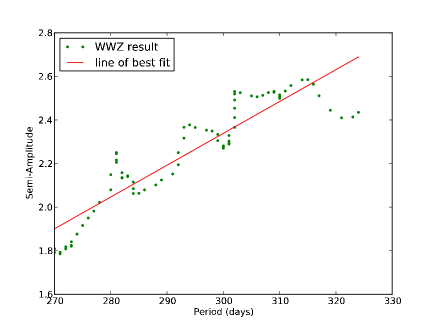
Figure 2: Amplitude versus period for R Aql (M6.5-9e). The positive correlation was suggested by Bedding et al. (2000) on the basis of the graphs of period and amplitude versus JD. The deviations from the straight-line fit suggest that there is one or more additional factors which affect the period and/or amplitude.

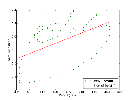
Figure 3: Amplitude versus period for S Ori (M6.5-7.5e). A positive correlation was suggested by Bedding et al. (2000) but it is clear that, although this graph shows such a correlation, the correlation is weak, presumably because of other processes which affect the period and/or amplitude.

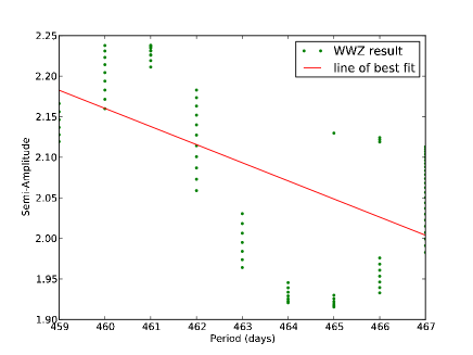
Figure 4: Amplitude versus period for GY Aql (M6e). The correlation is negative but the change in amplitude and period is very small, relative to their mean values.

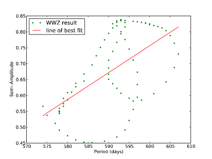
Figure 5: Amplitude versus period for S Aur (N0). The correlation is positive but weak and non-linear, indicating that other factors are important in determining the changes in period and/or amplitude.

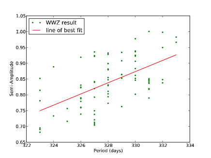
Figure 6: Amplitude versus period for S Cam (R8e). The correlation is positive but scattered and weak.

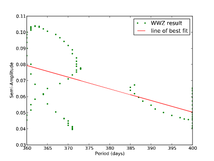
Figure 7: Amplitude versus period for DM Cep (M3D). The small amplitude makes any correlation meaningless.

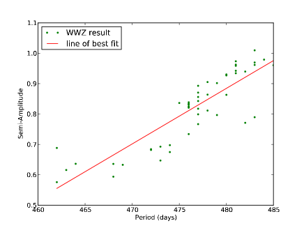
Figure 8: Amplitude versus period for SY Per (C6,4e). There is a significant positive correlation, with some deviations from this.

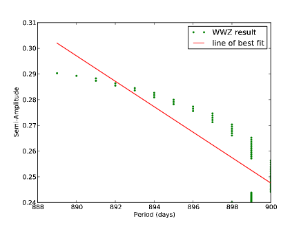
Figure 9: Amplitude versus period for UZ Per (M5II-III). The correlation is negative, but the amplitude and its change is very small.

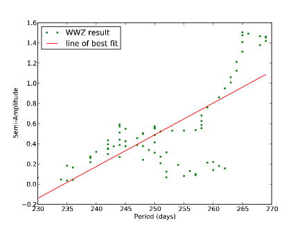
Figure 10: Amplitude versus period for W Tau (M6D). There is a positive correlation, with some deviations. The change in period is exceptionally large – 15 per cent.

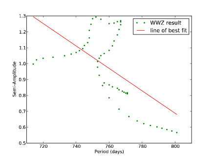
Figure 11: Amplitude versus period for VX Sgr (M5/6III or M4Iae). There is a negative correlation, but the relation is certainly not linear. This is not surprising in a star as complex as a red supergiant. The change in period is large – 10 per cent.

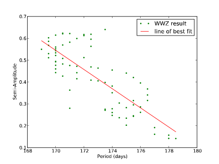
Figure 12: Amplitude versus period for DE Her (K0D), a yellow semi-regular variable star. There is a strong negative correlation, with significant deviations from this.

3.2. Red Supergiants

Table 2 presents the results of WWZ analysis for red supergiants. The notations used are the same as in Table 1. Seven red supergiants were studied. One had a negative correlation and six had a positive correlation between the semi-amplitude and the period.

Figure 11 is the semi-amplitude versus period plot for VX Sgr. VX Sgr has a long period which is a characteristic of supergiants. There is some negative correlation. However, the plot is non-linear and the line of best fit does not represent the plot well. This is not surprising, in view of the complexity of this class of stars.

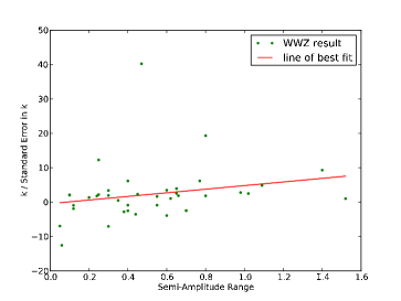
Figure 13: The relationship between k/$\sigma$ and the range in amplitude. There is a slight positive correlation.

3.3. Yellow Supergiants

Table 3 displays the result of WWZ analysis for yellow supergiants. The notations used are the same as in Table 1. Three yellow supergiants were studied and they all have a non-linear relationship between the semi-amplitude and the period, but only one is significant.

Figure 12 is the semi-amplitude versus period plot for DE Her. There is a weak negative correlation. The plot is non-linear and the line of best fit does not describe the plot in a meaningful way.

3.4. Summary Statistics

Figure 13 is a plot for $k/\sigma$ versus amplitude range. The slope of the linear fit was 0.19. The standard error in the slope was 3.29. The coefficient of correlation was 0.53. In both plots, the correlation is positive. It is not a strong correlation, but not weak either.

Table 1: Variability and WWZ results of pulsating red giants.

Star	P(d)	P Range	JD(1)	$\Delta$JD	A	A Range	k	$\sigma$	$k/\sigma$	$R$	Notes
RV And	165	38	2428000	28300	0.30	0.20-0.60	-2.54e-3	2.9e-3	-0.88	1.2e-1	3, 7
RY And	392	11	2427500	30000	1.69	0.68-2.20	1.89e-2	1.9e-2	1.00	1.3e-1	4, 7
R Aql	294	54	2415000	40000	2.25	1.79-2.59	1.46e-2	7.6e-4	19.32	9.1e-1	**, 1, 7
S Aql	143	8	2420000	36300	0.98	0.65-1.20	-1.45e-2	1.7e-2	-0.88	1.0e-1	4, 7
GY Aql	464	8	2447000	9300	2.35	1.90-2.20	-2.23e-2	3.2e-3	-7.05	6.0e-1	**, 8
RS Aqr	280	8	2430000	27500	2.73	2.58-2.97	-2.00e-2	7.2e-3	-2.80	3.6e-1	4, 7
T Ari	320	13	2428000	28300	0.91	0.70-1.35	1.59e-2	6.2e-3	2.55	3.2e-1	3, 5
S Aur	596	33	2416000	40300	0.61	0.45-0.85	8.46e-3	1.4e-3	6.15	5.7e-1	**, 3, 7
U Boo	204	10	2420000	49300	0.62	0.35-0.80	1.62e-2	7.0e-3	2.32	2.6e-1	3, 7
V Boo	887	50	2415000	40000	0.31	0.06-0.50	-3.43e-3	9.7e-4	-3.53	3.7e-1	*, 3, 5
RV Boo	144	29	2434000	22300	0.09	0.05-0.15	1.16e-3	5.7e-4	2.04	1.9e-1	3, 7
S Cam	327	10	2417000	39300	0.34	0.23-1.00	1.77e-2	2.9e-3	6.18	5.7e-1	**, 3, 7
RY Cam	134	6	2435000	21300	0.16	0.10-0.40	1.99e-2	5.9e-3	3.38	3.1e-1	*, 4, 7
T Cnc	488	19	2417000	39300	0.34	0.23-0.47	2.89e-3	1.6e-3	1.78	2.0e-1	3, 7
RT Cap	400	75	2417000	39300	0.31	0.25-0.45	4.52e-4	3.4e-4	1.35	4.5e-4	3, 7
T Cen	91	19	2413000	43300	0.62	0.50-1.20	-4.51e-2	1.8e-2	-2.47	2.6e-1	4, 7
DM Cep	367	40	2435000	21300	0.12	0.05-0.10	-7.26e-4	1.0e-4	-6.94	5.6e-1	**, 4, 7
T CMi	321	23	2415000	40000	1.86	1.24-2.27	1.25e-2	5.0e-3	2.50	2.7e-1	4, 5
RS CrB	331	7	2435000	21300	0.19	0.13-0.38	7.79e-3	3.5e-3	2.21	2.1e-1	5, 7
BH Cru	518	38	2440000	10000	1.21	0.91-1.38	1.20e-2	3.0e-4	40.24	9.8e-1	**, 1
T CVn	291	15	2415000	40000	0.83	0.57-1.27	-1.59e-2	6.5e-3	-2.44	6.5e-3	3, 7
RU Cyg	234	14	2415000	40000	0.38	0.11-0.77	1.33e-2	7.1e-3	1.87	2.1e-1	3, 7
V460 Cyg	160	15	2435000	21300	0.08	0.04-0.14	2.51e-3	1.2e-3	2.12	2.0e-1	3, 7
V930 Cyg	247	43	2442000	14300	0.72	0.30-0.70	-5.83e-3	2.3e-3	-2.52	2.9e-1	3, 7
EU Del	62	25	2435000	21300	0.08	0.05-0.17	-1.20e-3	1.3e-3	-0.93	9.0e-2	3, 7
SW Gem	700	117	2427500	28800	0.10	0.05-0.35	1.55e-3	8.0e-4	1.94	2.5e-1	3, 7
RR Her	250	12	2435000	21300	0.54	0.10-0.70	1.33e-2	3.8e-3	3.48	3.2e-1	*, 3, 5
RT Hya	255	29	2415000	41300	0.06	0.04-0.16	9.30e-3	5.1e-3	1.83	2.0e-1	3, 7
U Hya	791	98	2420000	36300	0.06	0.04-0.16	-2.22e-4	1.2e-4	-1.90	2.2e-1	3, 7
U LMi	272	31	2427500	30000	0.50	0.23-0.85	3.98e-3	3.7e-3	1.07	1.4e-1	3, 7
X Mon	148	9	2415000	41300	0.59	0.25-0.85	-3.04e-2	7.8e-3	-3.90	4.0e-1	*, 4, 7
S Ori	422	36	2415000	40000	1.93	0.30-2.39	1.52e-2	3.1e-3	4.85	4.9e-1	*, 3, 5
S Pav	387	11	2415000	40000	0.70	0.30-1.29	2.38e-2	8.6e-3	2.77	2.9e-1	3, 7
Y Per	251	11	2415000	40000	0.72	0.34-0.99	2.49e-2	6.3e-3	3.95	4.1e-1	*, 3, 7
SY Per	477	23	2446000	10300	0.89	0.67-0.92	1.83e-2	1.5e-3	12.26	8.7e-1	**, 1
UZ Per	850	11	2448000	8300	0.25	0.23-0.29	-4.95e-3	3.9e-4	-12.55	8.1e-1	**, 2
W Tau	243	39	2415000	41300	0.27	0.10-1.50	3.15e-2	3.4e-3	9.31	7.2e-1	**, 1
V UMa	198	42	2420000	36300	0.19	0.15-0.50	5.71e-4	1.1e-3	0.50	6.0e-2	3, 7
SS Vir	361	17	2420000	36300	0.82	0.60-1.15	4.56e-3	2.8e-3	1.64	1.9e-1	3, 5

Table 2: Variability and WWZ results of pulsating red supergiants.

Star	P(d)	P Range	JD(1)	$\Delta$JD	A	A Range	k	$\sigma$	$k/\sigma$	$R$	Notes
BO Car	337	20	2443000	14000	0.13	0.07-0.21	-5.6e-3	1.3e-3	-4.45	4.5e-1	*, 2, 7
PZ Cas	846	24	2440000	15000	0.24	0.13-0.50	6.5e-3	1.4e-3	4.66	4.6e-1	*, 3, 5
BC Cyg	703	25	2440000	15000	0.30	0.14-0.51	7.6e-3	2.1e-3	3.71	3.8e-1	*, 3, 5
W Ind	194	45	2443000	14000	0.40	0.95-1.09	-9.0e-4	1.4e-3	-0.63	7.0e-2	3, 7
S Per	809	44	2420000	35000	0.57	0.33-0.85	-9.1e-5	1.4e-3	-0.06	7.5e-3	3, 7
W Per	489	87	2415000	40000	0.35	0.19-0.48	-1.0e-4	3.3e-4	-0.31	3.4e-2	3, 7
VX Sgr	760	87	2427500	30000	0.73	0.57-1.30	-7.1e-3	1.3e-3	-5.36	5.8e-1	**, 3, 7

Table 3: Variability and WWZ results of pulsating yellow supergiants.

Star	P(d)	P Range	JD(1)	$\Delta$JD	A	A Range	k	$\sigma$	$k/\sigma$	$R$	Notes
AV Cyg	88	5	2430000	27500	0.37	0.12-0.56	-1.0e-2	1.4e-2	-0.73	9.9e-2	3, 7
DE Her	173	10	2442500	12500	0.42	0.14-0.64	-4.4e-2	4.1e-3	-10.77	7.9e-1	**, 3, 7
RS Lac	238	2	2427500	30000	0.72	0.35-1.03	7.4e-2	5.3e-2	1.40	1.8e-1	4, 7

3.4. Notes on Individual Stars.

RY And: There are some sparse regions of data in between dense regions.

GY Aql: The data are sparse.

R Aql: The data are sparse before 2420000. There is an outlier in period in the beginning.

S Aql: There is an abrupt change in period at the end of the data.

RV Boo: The period is not smooth.

RY Cam: The period is not smooth.

RT Cap: The data are sparse near JD = 2430000. There is an abrupt change in period in the middle.

BO Car: The data are sparse before JD = 2443000.

T Cen: The period is not smooth. The data are sparse near JD = 2430000. There is an abrupt change in period in the middle.

DM Cep: The data are sparse between JD = 2440000 and JD = 2442500. There is an abrupt change in period in the middle.

V460 Cyg: The period is not smooth.

V930 Cyg: The data are sparse before JD = 2445000. There is an outlier in period in the beginning.

EU Del: The period and the semi-amplitude are not smooth. There are two outliers in the light curve.

SW Gem: There is an abrupt change in the middle.

RR Her: The period and the semi-amplitude are not smooth.

RT Hya: There is an abrupt change in period. The semi-amplitude is not smooth.

U Hya: The data are sparse near JD = 2430000 There is an abrupt change in period in the middle.

W Ind: The data are sparse near JD = 2452500. There is an abrupt change in period and amplitude at the end.

U LMi: There is an abrupt change of period at the end.

X Mon: The period and the semi-amplitude are not smooth.

S Ori: The data are sparse before 2420000.

S Pav: The data are sparse from JD = 2420000 to JD = 2427000.

S Per: The data are sparse before JD = 2420000.

SY Per: The data are sparse before JD = 2448000.

VX Sgr: There is an abrupt change in period in the beginning.

W Per: There is an abrupt change in period in the beginning.

W Tau: There is an abrupt change in period in the middle.

4. Discussion

There are a variety of mechanisms which could cause period (or amplitude) changes in pulsating red giants and supergiants, and other cool, luminous stars: evolution, random cycle-to-cycle fluctuations, helium shell flashes, or simply the complexity of a star with large convective cells which is rotating and losing mass. Nevertheless: if we restrict our attention to stars whose amplitude and amplitude changes are sufficiently large, and whose amplitude versus period relation has a statistically significant linear slope, then 9 of 11 pulsating red giants show a period which increases with increasing amplitude. Choosing slightly differently: among stars with amplitudes greater than 1.0 mag, and significant changes in amplitude, 10 of 12 have a positive correlation between amplitude and period. This is not to say, of course, that the period change is caused by the amplitude change.

We must also remember that the visual light curve is not a bolometric light curve and that, for red stars, the visual band is especially sensitive to temperature, which may not have a direct effect on the pulsation period.

5. Conclusions

In stars with a variable pulsation amplitude, does an increase in pulsation amplitude result in an increase in period? The majority of the almost-50 pulsating stars in our sample do not show a linear relation between the instantaneous period and amplitude. Clearly, there are other processes which affect the period and amplitude. But, of the dozen stars which show sufficiently large amplitude and amplitude change, 75-80% show a positive correlation between the instantaneous amplitude and period.

Acknowledgements

We thank the hundreds of AAVSO observers who made the observations which were used in this project, and we thank the AAVSO staff for processing and archiving the measurements. We also thank the team which developed the VSTAR package, and made it user-friendly and publicly available. We are especially grateful to Professor Tim Bedding for suggesting this project in the first place. This project made use of the SIMBAD database, which is operated by CDS, Strasbourg, France.

References

Bedding, T.R., Conn, B.C., and Zijlstra, A.A., 2000, in The Impact of Large-Scale Surveys on Pulsating Star Research, eds. L. Szabados and D.W. Kurtz, ASP Conf. Ser. 203, Astronomical Society of the Pacific, San Francisco, 96.

Benn, D. 2013, VSTAR data analysis software (http://www.aavso.org/node/803).

Eddington, A.S. and Plakidis, S., 1929, Mon. Not. Roy. Astron. Soc., 90, 65.

Kiss, L.L., et al., 2006, Mon. Not. Roy. Astron. Soc., 372, 1721.

Percy, J.R. and Colivas, T., 1999, Publ. Astron. Soc. Pacific, 111, 94.

Percy, J.R. and Abachi, R., 2013, JAAVSO, 41, 193.

Percy, J.R., and Khatu, V., 2014, JAAVSO, in press.

Percy, J.R., and Kim, R., 2014, http://arxiv.org/abs/1405.6993

Zijlstra, A.A., et al., 2004, Mon. Not. Roy. Astron. Soc., 352, 325.