Entropy and its discontents:
A note on definitions

Abstract

The routine definitions of Shannon entropy for both discrete and continuous probability laws show inconsistencies that make them not reciprocally coherent. We propose a few possible modifications of these quantities so that 1) they no longer show incongruities, 2) they go one into the other in a suitable limit as the result of a renormalization. The properties of the new quantities would slightly differ from that of the usual entropies in a few other respects

PACS: 02.50.Cw, 05.45.Tp

MSC: 94A17, 54C70

Key words: Shannon entropy; continuous and discrete probability laws; renormalization

1 Introduction

As it is usually defined, the Shannon entropy of a discrete law $p_{k}=\bm{P}\left\{{x_{k}}\right\}$ associated to the values $x_{k}$ of some random variable is

$$H=-\sum_{k}p_{k}\ln p_{k}$$ (1)

and apparently is a non negative, dimensionless quantity. As a matter of fact however it does not depend on all the details of the distribution: for instance only the $p_{k}$ are relevant, while the $x_{k}$ play no role at all. This means that if we modify our distribution just by moving the $x_{k}$, the entropy is left the same: this entails among others that $H$ does not always change along with the variance (or other typical parameters) of the distribution which instead is contingent on the $x_{k}$ values. In particular $H$ is invariant under every linear transformation $ax_{k}+b$ (centering and rescaling) of the random quantities: in this sense every type of laws [1] is isoentropic. Surprisingly enough, despite the unsophistication of definition (1), and beyond a few elementary examples, explicit formulas displaying the dependence of the entropy $H$ from the parameters of the most common discrete distributions are not known. If for instance we take the entropy $H$ of the binomial distributions $\mathfrak{B}_{n,p}$ with

$$x_{k}=k=0,1,\ldots,n\qquad\quad p_{k}=\binom{n}{p}p^{k}(1-p)^{n-k}$$ (2)

although it would always be possible to calculate the entropy $H$ for every particular example, no general formula giving its explicit dependence from $n$ and $p$ is available, and only its asymptotic behavior for large $n$ is known in the literature [2, 3]:

$$H\left[\mathfrak{B}_{n,p}\right]=\frac{1}{2}\,\ln\left[2\pi enp(1-p)\right]+\frac{4p(1-p)-1}{12np(1-p)}+O\left(\frac{1}{n^{2}}\right)$$ (3)

Remark moreover that, while this formula explicitly contains $np(1-p)$ namely the variance of $\mathfrak{B}_{n,p}\,$, it is easy to recognize that – as long as we leave untouched the $n$ probabilities $p_{k}$ – the entropy $H\left[\mathfrak{B}_{n,p}\right]$ remains the same when we change the variance by moving the points $x_{k}$ away from their usual locations $x_{k}=k$. In particular this is true for the standardized (centered, unit variance) binomial $\mathfrak{B}_{n,p}^{*}$ with

$$x_{k}=\frac{k-np}{\sqrt{np(1-p)}}\qquad\quad k=0,1,\ldots,n$$ (4)

and same $p_{k}$ of (2) which entails $H\left[\mathfrak{B}_{n,p}\right]=H\left[\mathfrak{B}_{n,p}^{*}\right]$. All that hints to the fact that what seems to be relevant to the entropy is not the variance itself, but some other feature, possibly related to the shape of the distribution. In a similar vein, for the Poisson distributions $\mathfrak{P}_{\lambda}$ with

$$x_{k}=k=0,1,\ldots\qquad\quad p_{k}=e^{-\lambda}\frac{\lambda^{k}}{k!}$$ (5)

the entropy is

$$H\left[\mathfrak{P}_{\lambda}\right]=\lambda(1-\ln\lambda)+e^{-\lambda}\sum_{k=0}^{\infty}\frac{\lambda^{k}\ln k!}{k!}$$ (6)

with an asymptotic expression for large $\lambda$

$$H\left[\mathfrak{P}_{\lambda}\right]=\frac{1}{2}\,\ln\left(2\pi e\lambda\right)-\frac{1}{12\lambda}-\frac{1}{24\lambda^{2}}-\frac{19}{360\lambda^{3}}+O\left(\lambda^{-4}\right)$$ (7)

which explicitly contains the parameter $\lambda$ (also playing the role of the variance), but which is also completely independent from the values of the $x_{k}$’s. As a consequence a standardized Poisson distribution $\mathfrak{P}^{*}_{\lambda}$, with

$$x_{k}=\frac{k-\lambda}{\sqrt{\lambda}}$$ (8)

and same probabilities $p_{k}$, has the same entropy of $\mathfrak{P}_{\lambda}$, namely $H\left[\mathfrak{P}_{\lambda}\right]=H\left[\mathfrak{P}^{*}_{\lambda}\right]$.

When on the other hand we consider continuous laws with a pdf $f(x)$, the definition (1) no longer apply, and we are led to introduce another quantity commonly known as differential entropy (we acknowledge that this name could be misleading for an integral, but we will retain it in the following to abide a long established habit):

$$h=-\int_{\bm{R}}f(x)\ln f(x)\,dx$$ (9)

which in several respects differs from the entropy (1) of the discrete distributions. First of all explicit formulas of the entropy (9) are known for most of the usual laws: for example (see also Appendix A) the distributions $\mathfrak{U}(a)$ uniform on $[0,a]$ with $a>0$ have entropy

$$h\left[\mathfrak{U}\,\right]=\ln a$$ (10)

while for the centered, Gaussian laws $\mathfrak{N}(a)$ with variance $a^{2}$ we have

$$h\left[\mathfrak{N}\,\right]=\ln\left(a\sqrt{2\pi e}\right)$$ (11)

An exhaustive list of similar formulas for other families of laws is widely available in the literature, but even from these two examples only it is apparent that:

1. at variance with the discrete case, the differential entropies explicitly depend on a scaling parameter $a$, showing now a dependence either on the variance, or on some other dispersion index such as the inter quantile ranges (IQnR): this means in particular that the types of continuous laws are no longer isoentropic;

2. the differential entropies can take negative values when the parameters of the laws are chosen in such a way that the logarithm arguments fall below 1;

3. the logarithm arguments are not in general dimensionless quantities, in an apparent violation of the homogeneity rule that the scalar arguments of transcendental functions (as logarithms are) must be dimensionless quantities; this entails in particular that the entropy depends on the units of measurement

These three remarks make hence abundantly clear that something is inscribed in the definition (9) which is not present in the definition (1), and vice versa.

Finally the two definitions seem not to be reciprocally consistent in the sense that, when for instance a continuous law is weakly approximated by a sequence of discrete laws, we would like to see the entropies of the discrete distributions converging toward the entropy of the continuous one. That this is not the case is apparent from a few counterexamples. It is well known for instance that, for every $0<p<1$, the sequence of the standardized binomial laws $\mathfrak{B}_{n,p}^{*}$ weakly converges to the Gaussian $\mathfrak{N}(1)$ when $n\to\infty$; however, since the binomial probabilities $p_{k}$ are unaffected by a standardization, the entropies $H\left[\mathfrak{B}_{n,p}^{*}\right]$ still obey to formula (3), and hence their sequence diverges as $\ln\sqrt{n}$ instead of being convergent to the differential entropy of $\mathfrak{N}(1)$ which from (11) is $\ln\sqrt{2\pi e}$. In the same vein the cdf $F(x)$ of a uniform law $\mathfrak{U}(a)$ can be approximated by the sequence $F_{n}(x)$ of the discrete uniform laws $\mathfrak{U}_{n}(a)$ concentrated with equal probabilities $p_{1}=\ldots=p_{n}=\frac{1}{n}$ on the $n$ equidistant points $x_{1},\ldots,x_{n}$ where $x_{k}=k\Delta$ for $k=1,2,\ldots,n$, and $x_{k}-x_{k-1}=\Delta=\frac{a}{n}$ with $x_{0}=0$. However it is easy to see that

$$H[\mathfrak{U}_{n}]=-\sum_{k=1}^{n}\frac{1}{n}\ln\frac{1}{n}=\ln n$$ (12)

so that their sequence again diverge as $\ln n$, while the differential entropy $h[\mathfrak{U}\,]$ of the uniform law has the finite value (10).

As a consequence of these remarks, in the following sections we will propose a few elementary ways to change the two definitions (1) and (9) in order to possibly rid them of the said inconsistencies, and to make them reciprocally coherent without losing too much of the essential properties of the usual quantities. These new definitions, moreover, operate an effective renormalization of the said divergences so that now, when a continuous law is weakly approximated by a sequence of discrete laws, also the entropies of the discrete distributions converge toward the entropy of the continuous one. A few additional points with examples and explicit calculations are finally collected in the appendices. It must be clearly stated at this point, however, that we do not claim here that the Shannon entropy is somehow ill-defined in itself: we rather point out a few reciprocal inconsistencies of the different manifestations of this time-honored concept, and we try to attune them in such a way that every probability distribution (either discrete, or continuous) would now be treated on the same foot

2 Entropy for continuous laws

Let us begin with some remarks about the differential entropy for continuous laws with a pdf $f(x)$: the simplest ways to achieve the essential of our aims would be to adopt some new definition of the type

$$-\int_{\bm{R}}f(x)\ln\left[\kappa f(x)\right]\,dx=h-\ln\kappa$$ (13)

where $\kappa$ is any parameter of the law $f(x)$ with the same dimensions of $x$, and with a finite and strictly positive value for every non degenerate law. To this end the first idea which comes to the fore consists in taking the standard deviation $\sigma$ to play the role of $\kappa$ in (13), but it is also apparent that this choice would restrict our definition only to the continuous laws with finite second momentum leaving out many important cases. A strong alternative candidate for the role of $\kappa$ could instead be some interquantile range (IQnR) which can represent a measure of the dispersion even when the variance does not exist. In the following we will analyze a few possible choices for the parameter $\kappa$ along with their principal consequences

2.1 Interquantile range

The calculation of the IQnR goes through the use of the quantile function $Q(p)$, namely the inverse cumulative distribution function (cdf). In order to take into account possible jumps and flat spots of a given cdf $F(x)$, the quantile function is usually defined as

$$Q(p)=\inf\{x\in{\bm{R}}:p\leq F(x)\}\qquad\quad 0\leq p\leq 1$$ (14)

In the case of continuous laws (no jumps), however, this can be reduced to

$$Q(p)=\inf\{x\in{\bm{R}}:p=F(x)\}$$ (15)

and when $F(x)$ is also strictly increasing (no flat spots) we finally have

$$Q(p)=F^{-1}(p)$$ (16)

It is apparent then that $Q(p)$ jumps wherever $F(x)$ has flat spots, while it has flat spots wherever $F(x)$ jumps. The IQnR function is then defined as

$$\varrho(p)=Q(1-p)-Q(p)\qquad\quad 0<p<\frac{1}{2}$$ (17)

and the classical interquartile range (IQrR) is just the particular value

$$\varrho\left(\frac{1}{4}\right)=Q\left(\frac{3}{4}\right)-Q\left(\frac{1}{4}\right)$$ (18)

The IQnR $\varrho(p)$ is a non increasing function of $p$, and for continuous laws (since $Q(p)$ has no flat spots) it is always well defined and never vanishes so that one of its values can be safely used to play a role in the definition of $\kappa$ in (13). Of course, when a law has also a finite second momentum, the IQnR $\varrho$ and the standard deviation $\sigma$ are both well defined and the ratio $\gamma=\varrho/\sigma$ often has the same for entire families of laws. We now propose to adopt a new form for the entropy of continuous laws which – by making use, instead of the variance, of some particular value of IQnR that we will denote $\widetilde{\varrho}$ – will encompass even the case of the laws without a finite second momentum:

$$\widetilde{h}=-\int_{\bm{R}}f(x)\ln\left[\widetilde{\varrho}\,f(x)\right]\,dx=h-\ln\widetilde{\varrho}$$ (19)

In particular for the continuous laws we can simply take $\widetilde{\varrho}=\varrho\left(\frac{1}{4}\right)$, the IQrR

Despite the minimality of this change of definition, however, the new entropy $\widetilde{h}$ has properties slightly different from $h$. It is shown by the examples of the Appendix A that – at variance with the usual differential entropy $h$ – this new entropy $\widetilde{h}$ has neither a minimum, nor a maximum value because, according to the particular continuous law considered, it takes every possible real value, both positive and negative. In this respect we must instead recall the well known property of the Gaussian laws $\mathfrak{N}(a)$ which qualify as the laws with the maximum differential entropy $h$ among all the other continuous laws with the same variance $\sigma^{2}$. It is apparent then that within our new definition (19) this special position of the Gaussian laws will simply be lost.

The adoption of (19) however brings several benefits that will also be made apparent in the examples of the Appendix A: first of all the argument of the logarithm is now by definition a dimensionless quantity so that the value of $\widetilde{h}$ becomes invariant under change of measurement units. Second, the new entropy $\widetilde{h}$ will no longer depend on the value of some scaling parameters linked to the variance: its values are determined by the form of the distribution, rather than by its actual numerical dispersion, and will be the same for entire families of laws. When in fact the variables are subject to some linear transformation $y=ax+b$ (with $a>0$, as in the changes of unit of measurement) the differential entropy $h$ changes with the new pdf according to

$$-\int_{\bm{R}}\frac{1}{a}f\left(\frac{y-b}{a}\right)\ln\left[\frac{1}{a}f\left(\frac{y-b}{a}\right)\right]\,dy=-\int_{\bm{R}}f(x)\ln f(x)\,dx+\ln a$$

namely it is explicitly dependent from the scaling parameter $a$, while it is independent from the centering parameter $b$. It is apparent moreover that, according to these remarks, also the quantile function of the transformed cdf

$$F\left(\frac{x-b}{a}\right)$$

is changed into $aF^{-1}(p)+b=aQ(p)+b$ so that any IQnR is modified according to $a\varrho(p)$, namely it will be sensitive again only to the scaling parameter $a$, but not to the centering one. As a consequence the modifications of both $h$ and $\widetilde{\varrho}$ under a linear transformation of the variables are apparently such that they cancel out reciprocally so that $\widetilde{h}$, as defined in (19), is always left unchanged: this means in particular that the types of laws are isoentropic

2.2 Variance and scaling parameters

By restricting ourselves to the continuous laws with finite second momentum and standard deviation $\sigma$, an alternative redefinition of the differential entropy could be considered as

$$-\int_{\bm{R}}f(x)\ln\left[\sigma f(x)\right]\,dx=h-\ln\sigma$$ (20)

This form of differential entropy would bring the same benefits of $\widetilde{h}$: the argument of the logarithm is dimensionless, and it will no longer depend on the value of scaling parameters. Since however the dimensional parameter is the standard deviation, it is possible to show that the Gaussian laws would keep now their usual role of maximum entropy laws, and this suggests to propose a further possible change of definition as (please remark the change of sign)

$$\widehat{h}=\int_{\bm{R}}f(x)\ln\left[\sigma\sqrt{2\pi e}\,f(x)\right]\,dx=\ln\left(\sigma\sqrt{2\pi e}\right)-h$$ (21)

As shown in the Appendix A, all the Gaussian laws $\mathfrak{N}(a)$ will now have $\widehat{h}[\mathfrak{N}]=0$ and – because of the change of sign – this value will now represent the minimum for all the other laws, irrespective of their variance: as a consequence the entropy $\widehat{h}$ of all the continuous distributions with finite variance will now be non negative, as for the entropy $H$ of the discrete laws.

For laws lacking a finite second momentum (as the Cauchy laws) we would have no $\widehat{h}$ entropy because these distributions have no variance to speak about: this is an apparent shortcoming presented by the definition (21) of $\widehat{h}$, and to go around this weakness we introduced our definition (19) of $\widetilde{h}$ by exploiting the properties of the IQnR $\varrho(p)$ which are always well defined for every possible distribution. It would be interesting to remark, however, not only that these are not the only two possible choices, but also that even seeming harmless modifications can imply slightly different properties. For instance, by going back to the remarks at the end of the Section 2.1, it is well known that by linear transformation of the variables (with $a>0$ to simplify) every continuous law $f(x)$ spans a type of continuous laws

$$\frac{1}{a}f\left(\frac{x-b}{a}\right)$$

As already pointed out, the centering parameter $b$ has no influence on the value of the entropy, while the scaling parameter $a$ would change the differential entropy $h$ of definition (9) by an additional $\ln a$. As a consequence by simply adopting as a new definition

$$\overline{h}=-\int_{\bm{R}}f(x)\ln\left[af(x)\right]\,dx=h-\ln a$$ (22)

where $a$ is the parameter locating the law within its type, we would get an entropy invariant for rescaling. It is apparent that the definition (22) considers $a$ just as a parameter, and not as a measure of dispersion, and it is interesting to notice that it also entails a few consequences shown in the examples of the Appendix A. In particular we now have that the entropy $\overline{h}$ takes again all the (positive and negative) real values and hence that there is no such a thing as a maximum entropy distribution as in the case of the $\widetilde{h}$ entropy

3 Entropy for discrete laws

We could now naively extend to the discrete laws our previous re-definitions simply by taking $H-\ln\kappa$, with $H$ given by (1), and with a suitable choice of $\kappa$, but in so doing we would miss a chance to reconcile the two forms (discrete and continuous) of our entropy in some limit behavior. We find then more convenient to introduce some further changes that for the sake of generality we will discuss in the settings of the Section 2.1 where $\kappa$ is an IQnR

3.1 Renormalization

In order to extend the definition (19) to the discrete distributions we must first remark that, at variance with the continuous case, now the IQrR $\varrho\left(\frac{1}{4}\right)$ can vanish and hence can not be immediately adopted as $\kappa$ in our definitions. For the discrete laws in fact $F(x)$ makes jumps and hence $Q(p)$ has flat spots so that $\varrho(p)$ can be zero for some values of $p$, and in particular this can happen also for $p=\frac{1}{4}$. If however our distributions are purely discrete (a few remarks about the more general case of mixtures can be found in the Appendix B) $\varrho(p)$ is a non increasing function of $p$ which change values only by jumping, and which is constant between subsequent jumps. As a consequence, with the only exception of the degenerate laws (which have a constant $Q(p)$, and hence a $\varrho$ vanishing for every $p$), $\varrho(p)$ certainly takes non zero values for some $0<p\leq\frac{1}{4}$, even when $\varrho\left(\frac{1}{4}\right)=0$. We can then use in our definitions as dimensional constant $\widetilde{\varrho}$ the smallest, non zero IQnR larger or equal to the IQrR $\varrho\left(\frac{1}{4}\right)$: more precisely, if $\mathcal{P}$ is the set of all the values of $\varrho(p)$ for $0<p\leq\frac{1}{4}$, and $\mathcal{P}_{0}=\mathcal{P}\backslash\{0\}$, we will take $\widetilde{\varrho}=\min\mathcal{P}_{0}>0$. Remark that in particular we again have $\widetilde{\varrho}=\varrho\left(\frac{1}{4}\right)$ whenever the IQrR does not vanish.

We start by remarking that if $F(x)$ is the cumulative distribution function of a discrete distribution concentrated on $x_{k}$ with probabilities $p_{k}$ for $k=1,2\ldots\,$, by taking

$$\Delta x_{k}=x_{k}-x_{k-1}\qquad\quad\Delta F_{k}=F(x_{k})-F(x_{k-1})=p_{k}\qquad\quad k=1,2,\ldots$$

(with $x_{0}<x_{1}$ and hence $F(x_{0})=0$: for instance $x_{0}=x_{1}-\inf_{k\geq 2}\Delta x_{k}$ so that $\Delta x_{1}=\inf_{k\geq 2}\Delta x_{k}$) we see first that the definition (1) can be immediately recast in the form

$$H=-\sum_{k\geq 1}\Delta F_{k}\ln\Delta F_{k}$$

Since on the other hand many typical discrete distributions (binomial, Poisson $\ldots$) describe counting experiments, in many instances we have $\Delta x_{k}=1$ and in these cases (since $\Delta x_{k}$ is also dimensionless) we could also write

$$H=-\sum_{k\geq 1}\Delta F_{k}\ln\frac{\Delta F_{k}}{\Delta x_{k}}$$

By comparing this expression with the definition of differential entropy (9), and by recalling that for a continuous distribution we have $f(x)=F\,^{\prime}(x)$, we are led to propose as new definition of the entropy of a discrete law the quantity

$$\widetilde{H}=-\sum_{k\geq 1}\frac{\Delta F_{k}}{\Delta x_{k}}\ln\left(\widetilde{\varrho}\,\frac{\Delta F_{k}}{\Delta x_{k}}\right)\Delta x_{k}=H+\sum_{k\geq 1}p_{k}\ln\Delta x_{k}-\ln\widetilde{\varrho}$$ (23)

In general, even for the discrete distributions, $\Delta x_{k}$ is not dimensionless, but apparently this is compensated by means of $\widetilde{\varrho}$. This definition (23) has properties which are similar to that of the new differential entropy defined in the previous section, but the main benefit of this new formulation is that now – as it will be discussed in the subsequent section – the differential $\widetilde{h}$ entropy of a continuous law (19) can be recovered as a limit of the entropies $\widetilde{H}$ of a sequence of approximating, discrete laws. In fact the new definition (23) effectively renormalizes the traditional entropy $H$ in such a way that the asymptotic divergences pointed out in the Section 1 are exactly compensated by means of our dimensional parameters. These conclusions hold also for a suitable extension of the alternative definitions (21) and (22) respectively of $\widehat{h}$ and $\overline{h}$

3.2 Convergence

We will discuss in this section a few particular examples showing that the two quantities $\widetilde{h}$ of (19) and $\widetilde{H}$ in (23) are no longer disconnected concepts, as happens for the usual definitions (1) and (9). Let us consider first the case of the binomial laws $\mathfrak{B}_{n,p}$ and of their standardized versions $\mathfrak{B}_{n,p}^{*}$ already introduced in the Section 1: we know that $H[\mathfrak{B}_{n,p}]=H[\mathfrak{B}_{n,p}^{*}]$ and that both these entropies diverge as $\ln\sqrt{n}$ when $n\to\infty$. On the other hand, since $\Delta x_{k}=1$ for $\mathfrak{B}_{n,p}$, from (23) we get

$$\widetilde{H}[\mathfrak{B}_{n,p}]=H[\mathfrak{B}_{n,p}]-\ln\widetilde{\varrho}$$

For binomial laws with fixed $p$, and $n$ large enough, the IQrR does not vanish so that $\widetilde{\varrho}=\varrho\left(\frac{1}{4}\right)$ and, by introducing the ratio

$$\gamma=\frac{\varrho\left(\frac{1}{4}\right)}{\sigma}$$ (24)

we have

$$\widetilde{\varrho}=\gamma\sigma=\gamma[\mathfrak{B}_{n,p}]\sqrt{np(1-p)}$$

and hence

$$\widetilde{H}[\mathfrak{B}_{n,p}]=H[\mathfrak{B}_{n,p}]-\ln\widetilde{\varrho}=H[\mathfrak{B}_{n,p}]-\ln\left(\gamma[\mathfrak{B}_{n,p}]\sqrt{np(1-p)}\right)$$

From (3) for large $n$, since from the binomial limit theorem we have $\gamma[\mathfrak{B}_{n,p}]\overset{n}{\longrightarrow}\gamma[\mathfrak{N}]$, while from (27) and (29) in Appendix A it is

$$\gamma[\mathfrak{N}]=\Phi^{-1}\left(\frac{3}{4}\right)-\Phi^{-1}\left(\frac{1}{4}\right)$$

by taking into account (30) of Appendix A, we finally get

$$\widetilde{H}[\mathfrak{B}_{n,p}] = \frac{1}{2}\,\ln\left[2\pi enp(1-p)\right]+\frac{4p(1-p)-1}{12np(1-p)}+O\left(\frac{1}{n^{2}}\right)-\ln\left[\gamma[\mathfrak{B}_{n,p}]\sqrt{np(1-p)}\right]$$

$$= -\ln\left(\frac{\gamma[\mathfrak{B}_{n,p}]}{\sqrt{2\pi e}}\right)+\frac{4p(1-p)-1}{12np(1-p)}+O\left(\frac{1}{n^{2}}\right)\overset{n}{\longrightarrow}-\ln\left(\frac{\gamma[\mathfrak{N}]}{\sqrt{2\pi e}}\right)=\widetilde{h}[\mathfrak{N}]$$

which is a first example of the convergence of entropies to differential entropies in the framework of the new definitions. The same result is achieved for $\widetilde{H}[\mathfrak{B}_{n,p}^{*}]$ because now $\sigma=1$, so that $\widetilde{\varrho}=\gamma[\mathfrak{B}_{n,p}]$ while from (4) we have for every $k$

$$\Delta x_{k}=\frac{1}{\sqrt{np(1-p)}}$$

and hence from (23) we get

$$\widetilde{H}[\mathfrak{B}_{n,p}^{*}]=H[\mathfrak{B}_{n,p}^{*}]-\ln\left(\gamma[\mathfrak{B}_{n,p}^{*}]\sqrt{np(1-p)}\right)$$

On the other hand we know that $H[\mathfrak{B}_{n,p}^{*}]=H[\mathfrak{B}_{n,p}]$, so that from $\gamma[\mathfrak{B}_{n,p}^{*}]\overset{n}{\longrightarrow}\gamma[\mathfrak{N}]$ we get again

$$\widetilde{H}[\mathfrak{B}_{n,p}^{*}]\overset{n}{\longrightarrow}\widetilde{h}[\mathfrak{N}]$$

Similar results hold for the Poisson laws $\mathfrak{P}_{\lambda}$: we already remarked in the Section 1 that, while $\mathfrak{P}^{*}_{\lambda}\to\mathfrak{N}(1)$ for $\lambda\to\infty$, the entropies $H[\mathfrak{P}_{\lambda}]=H[\mathfrak{P}^{*}_{\lambda}]$ diverge as $\ln\sqrt{\lambda}$. It could be shown instead that both $\widetilde{H}[\mathfrak{P}_{\lambda}]$ and $\widetilde{H}[\mathfrak{P}^{*}_{\lambda}]$ graciously converge to $\widetilde{h}[\mathfrak{N}]$ because now we respectively have $\sigma=\sqrt{\lambda}$ and $\Delta x_{k}=\frac{1}{\sqrt{\lambda}}$

In a similar way for the discrete uniform distributions $\mathfrak{U}_{n}(a)$ introduced in the Section 1 we now have

$$x_{k}=\frac{ka}{n}\quad\qquad\Delta x_{k}=\frac{a}{n}\quad\qquad p_{k}=\frac{1}{n}\quad\qquad k=1,\ldots,n$$

so that, since $\widetilde{\varrho}[\mathfrak{U}_{n}]$ is the IQrR $\varrho_{\frac{1}{4}}$ again, from (12) and (23) we get

$$\widetilde{H}[\mathfrak{U}_{n}]=\ln n+\ln\frac{a}{n}-\ln\widetilde{\varrho}[\mathfrak{U}_{n}]=\ln a-\ln\widetilde{\varrho}[\mathfrak{U}_{n}]$$

If we then remember from (32) that $\widetilde{\varrho}[\mathfrak{U}_{n}]\overset{n}{\longrightarrow}\widetilde{\varrho}[\mathfrak{U}]=\frac{a}{2}$, we finally get from (33)

$$\widetilde{H}[\mathfrak{U}_{n}]\overset{n}{\longrightarrow}\ln a-\ln\widetilde{\varrho}[\mathfrak{U}]=\ln a-\ln\frac{a}{2}=\ln 2=\widetilde{h}[\mathfrak{U}]$$

We are then allowed to conjecture that this is a generalized behavior: within the frame of our definitions (23) of $\widetilde{H}$ and (19) of $\widetilde{h}$, whenever – as in our previous examples – a sequence of purely discrete laws $\mathfrak{A}_{n}$ weakly converges to a continuous law $\mathfrak{A}$, then also $\widetilde{H}[\mathfrak{A}_{n}]\overset{n}{\longrightarrow}\widetilde{h}[\mathfrak{A}]$

4 Conclusions

We have proposed to modify both the usual definition (1) of the entropy $H$, and (9) of the differential entropy $h$ respectively into (23) and (19), namely within our most general notation

$$\widetilde{H} = -\sum_{k\geq 1}\frac{\Delta F_{k}}{\Delta x_{k}}\ln\left(\widetilde{\varrho}\,\frac{\Delta F_{k}}{\Delta x_{k}}\right)\Delta x_{k}=H-\ln\widetilde{\varrho}+\sum_{k\geq 1}p_{k}\ln\Delta x_{k}$$ (25)

$$\widetilde{h} = -\int_{\bm{R}}f(x)\ln\left[\widetilde{\varrho}\,f(x)\right]\,dx=h-\ln\widetilde{\varrho}$$ (26)

where in general $\widetilde{\varrho}$ coincides with the IQrR $\varrho\left(\frac{1}{4}\right)$ of the considered distribution, except when the IQrR vanishes (as can happen for discrete laws): in this last event $\widetilde{\varrho}$ is taken as the smallest non zero IQnR of the distribution. There are also several other possible re-definitions which essentially differ among them by the choice of the parameter $\kappa$ in (13), and by the set of their possible values. All these definitions, moreover, bypass the anomalies listed in the Section 1 and appear to go smoothly one into the other for suitable discrete-continuous limit. As a matter of fact the introduction of the dimensional parameter $\kappa$ effectively renormalizes the divergences that we would otherwise encounter in the limiting processes leading from discrete to continuous laws. Remark finally that the discrete form (25) can also be easily customized to fit with the entropy estimation from empirical data

We end the paper by pointing out that, despite extensive similarities, the new quantities such as $\widetilde{H}$ and $\widetilde{h}$ no longer have all the same properties of $H$ and $h$. For instance at the present stage we could neither prove, nor disprove (by means of some counterexample) that $\widetilde{H}\geq 0$ as for $H$. On the other hand the examples seem also to allow no room for $\widetilde{h}$-extremal distributions, as the normal laws were for the $h$ differential entropy. Remark however that these conclusions would be different by adopting the alternative definitions that are presented in the Section 2.2. While all these topics seem to be interesting fields of inquiry, it would also be important to extensively review what is preserved of all the well known properties of the usual definitions, and how to adapt further ideas such as relative entropy, mutual information and whatever else is today used in the information processing [4, 5]. This remarks emphasize the possibilities open by our seemingly naive changes: as a bid to connect two previous standpoints, in fact, our proposed definitions blend the properties of the older quantities, and in so doing can also break new ground. An extensive analysis of all the possible consequences both of the proposed definitions, and of their articulations will be the subject of a forthcoming paper, while on this topic we will at present limit ourselves just to point out that many relevant features of the entropy essentially derive from the properties of the logarithms which in any case play a central role also in the new definitions. Finally it would be stimulating to explore how – if at all – it is possible to make the new definitions compatible with other celebrated extensions of the classical entropies such as, for instance, that proposed by Tsallis [6], or the more recent cumulative residual entropy [7]

Appendix A Examples

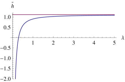
Figure 1: Entropy $\widetilde{h}[\mathfrak{G}_{\lambda}]$ for gamma laws

We begin by comparing the values of the two differential entropies $h$ and $\widetilde{h}$, respectively defined as (9) and (19), for the most common families of laws by neglecting the centrality parameters which are irrelevant for our purposes because both the entropies are independent from them.

For the Gaussian laws $\mathfrak{N}(a)$ with

$$f(x)=\frac{e^{-\frac{x^{2}}{2a^{2}}}}{a\sqrt{2\pi}}\qquad\quad\sigma=a\qquad\quad h[\mathfrak{N}]=\ln\left(a\sqrt{2\pi e}\right)$$ (27)

we know that

$$F(x)=\Phi\left(\frac{x}{a}\right)\quad\qquad\;\,\Phi(y)=\int_{-\infty}^{y}\frac{e^{-\frac{z^{2}}{2}}}{\sqrt{2\pi}}\,dz$$ (28)

$$Q(p)=a\Phi^{-1}(p)\qquad\quad\widetilde{\varrho}\,[\mathfrak{N}]=a\left[\Phi^{-1}\left(\frac{3}{4}\right)-\Phi^{-1}\left(\frac{1}{4}\right)\right]$$ (29)

and hence we immediately have from (19)

$$\widetilde{h}[\mathfrak{N}]=h[\mathfrak{N}]-\ln\widetilde{\varrho}\,[\mathfrak{N}]=\ln\frac{\sqrt{2\pi e}}{\Phi^{-1}\left(\frac{3}{4}\right)-\Phi^{-1}\left(\frac{1}{4}\right)}\approx 1.11959$$ (30)

For the laws $\mathfrak{U}(a)$ uniform on $[0,a]$ with (here $\vartheta(x)$ is the Heaviside function)

$$f(x)=\frac{\vartheta(x)-\vartheta(x-a)}{a}\qquad\quad\sigma=\frac{a}{\sqrt{12}}\qquad\quad h[\mathfrak{U}]=\ln a$$ (31)

we instead have

$$F(x)=\frac{x}{a}\qquad 0\leq x\leq a\qquad\qquad Q(p)=ap\qquad 0<p<1\qquad\quad\widetilde{\varrho}=\frac{a}{2}$$ (32)

so that

$$\widetilde{h}[\mathfrak{U}]=\ln a-\ln\frac{a}{2}=\ln 2\approx 0.693147$$ (33)

For the gamma laws $\mathfrak{G}_{\lambda}(a)$, $\lambda>0$ with

$$f(x)=\vartheta(x)\frac{x^{\lambda-1}e^{-\frac{x}{a}}}{a^{\lambda}\Gamma(\lambda)}\qquad\quad\sigma=a\sqrt{\lambda}\qquad\quad h[\mathfrak{G}_{\lambda}]=(1-\lambda)\psi(\lambda)+\ln\left[ae^{\lambda}\Gamma(\lambda)\right]$$ (34)

where

$$\psi(z)=\frac{\Gamma\,^{\prime}(z)}{\Gamma(z)}$$

we have

$$F(x)=\Gamma_{\lambda}\left(\frac{x}{a}\right)\qquad\quad\Gamma_{\lambda}(y)=1-\frac{\Gamma(\lambda,y)}{\Gamma(\lambda,0)}\qquad\quad\Gamma(\lambda,y)=\int_{y}^{\infty}t^{\lambda-1}e^{-t}dt$$

$$\qquad\qquad Q(p)=a\Gamma_{\lambda}^{-1}(p)\qquad\quad\widetilde{\varrho}=a\left[\Gamma_{\lambda}^{-1}\left(\frac{3}{4}\right)-\Gamma_{\lambda}^{-1}\left(\frac{1}{4}\right)\right]$$

and hence

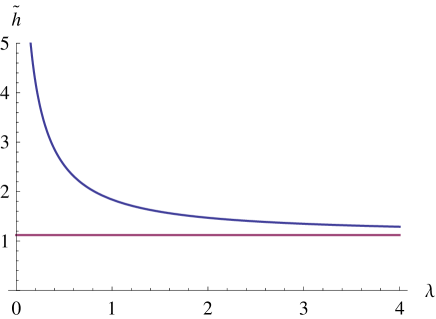
Figure 2: Entropy $\widetilde{h}[\mathfrak{T}_{\lambda}]$ for Student laws

$$\widetilde{h}[\mathfrak{G}_{\lambda}]=(1-\lambda)\psi(\lambda)+\ln\frac{e^{\lambda}\Gamma(\lambda)}{\Gamma_{\lambda}^{-1}\left(\frac{3}{4}\right)-\Gamma_{\lambda}^{-1}\left(\frac{1}{4}\right)}$$ (35)

which as a function of $\lambda$ is displayed in the Figure 1: this shows that $\widetilde{h}[\mathfrak{G}_{\lambda}]$ takes also negative values, that $\widetilde{h}[\mathfrak{G}_{\lambda}]\to-\infty$ for $\lambda\to 0$, and that $\widetilde{h}[\mathfrak{G}_{\lambda}]\uparrow\widetilde{h}[\mathfrak{N}]$ for $\lambda\to+\infty$. In particular for the exponential laws $\mathfrak{E}(a)=\mathfrak{G}_{1}(a)$ with

$$f(x)=\vartheta(x)\frac{e^{-\frac{x}{a}}}{a}\qquad\quad\sigma=a\qquad\quad h[\mathfrak{E}]=1+\ln a=\ln(ea)$$ (36)

we have

$$F(x)=\left(1-e^{-\frac{x}{a}}\right)\vartheta(x)\qquad\quad Q(p)=-a\ln(1-p)\qquad 0<p<1\qquad\quad\widetilde{\varrho}=a\ln 3$$

so that

$$\widetilde{h}[\mathfrak{E}]=1-\ln(\ln 3)\approx 0.905952$$ (37)

For the Laplace laws $\mathfrak{L}(a)$ with

$$f(x)=\frac{e^{-\frac{|x|}{a}}}{2a}\qquad\quad\sigma=a\sqrt{2}\qquad\quad h[\mathfrak{L}]=\ln(2ae)$$ (38)

we know that

$$\widetilde{\varrho}=2a\ln 2$$

and hence

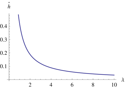
Figure 3: Entropy $\widehat{h}[\mathfrak{G}_{\lambda}]$ for the gamma laws

$$\widetilde{h}[\mathfrak{L}]=1-\ln\left(\ln 2\right)\approx 1.36651\geq\widetilde{h}[\mathfrak{N}]$$ (39)

Finally for the family of Student laws $\mathfrak{T}_{\lambda}(a)$, $\lambda>0$ with

$$f(x)=\frac{1}{aB\left(\frac{1}{2},\frac{\lambda}{2}\right)}\left(\frac{a^{2}}{a^{2}+x^{2}}\right)^{\frac{\lambda+1}{2}}\qquad\sigma=\frac{a}{\sqrt{\lambda-2}}\qquad\quad B(\alpha,\beta)=\frac{\Gamma(\alpha)\Gamma(\beta)}{\Gamma(\alpha+\beta)}$$ (40)

the variance exists only for $\lambda>2$, but the differential entropy is well defined for every $\lambda>0$

$$h[\mathfrak{T}_{\lambda}]=\frac{\lambda+1}{2}\left[\psi\left(\frac{\lambda+1}{2}\right)-\psi\left(\frac{\lambda}{2}\right)\right]+\ln\left[aB\left(\frac{1}{2},\frac{\lambda}{2}\right)\right]$$ (41)

For short the explicit form of the IQrR $\widetilde{\varrho}$ will not be explicitly given here. Since however the differential entropy $h[\mathfrak{T}_{\lambda}]$, and the IQRr $\widetilde{\varrho}\,[\mathfrak{T}_{\lambda}]$ are both proportional to the scaling parameter $a$, the entropy $\widetilde{h}[\mathfrak{T}_{\lambda}]$ will be independent from $a$, and as a function of $\lambda$ is displayed in the Figure 2 which shows that $\widetilde{h}[\mathfrak{T}_{\lambda}]$ takes always positive values larger than $\widetilde{h}[\mathfrak{N}]\approx 1.11959$, that $\widetilde{h}[\mathfrak{G}_{\lambda}]\to+\infty$ for $\lambda\to 0$, and that $\widetilde{h}[\mathfrak{G}_{\lambda}]\downarrow\widetilde{h}[\mathfrak{N}]$ for $\lambda\to+\infty$. In particular for the Cauchy laws $\mathfrak{C}(a)=\mathfrak{T}_{1}(a)$, without variance, with

$$\qquad\qquad\quad f(x)=\frac{1}{a\pi}\,\frac{a^{2}}{a^{2}+x^{2}}\qquad\quad h[\mathfrak{C}]=\ln\left(4\pi a\right)$$ (42)

$$F(x)=\frac{1}{2}+\frac{1}{\pi}\arctan\frac{x}{a}\quad\qquad Q(p)=a\tan\frac{(2p-1)\pi}{2}\quad\qquad\widetilde{\varrho}=2a$$ (43)

we have that

$$\widetilde{h}[\mathfrak{C}]=\ln(4\pi a)-\ln(2a)=\ln(2\pi)\approx 1.83788\geq\widetilde{h}[\mathfrak{N}]$$ (44)

A particular consequence of these example is that – as already remarked in the Section 2.1 – the entropy $\widetilde{h}$ has neither maximum, nor minimum value, and by suitably choosing the continuous law it can take every real value both positive and negative

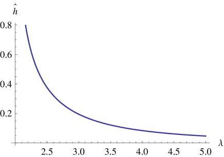
Figure 4: Entropy $\widehat{h}[\mathfrak{T}_{\lambda}]$ for Student laws with $\lambda>2$

Similar calculations can then be carried on also for the alternative entropy definition (21) of $\widehat{h}$ for laws endowed with a finite second momentum: we immediately get for the Gaussian laws

$$\widehat{h}[\mathfrak{N}]=\ln\left(a\sqrt{2\pi e}\right)-\ln\left(a\sqrt{2\pi e}\right)=0$$ (45)

and for the uniform laws

$$\widehat{h}[\mathfrak{U}]=\ln\left(\frac{a}{\sqrt{12}}\sqrt{2\pi e}\right)-\ln a=\ln\sqrt{\frac{\pi e}{6}}\approx 0.1765$$ (46)

For the gamma laws we have now

$$\widehat{h}[\mathfrak{G}_{\lambda}]=\ln\left(a\sqrt{2\pi e\lambda}\right)-(1-\lambda)\psi(\lambda)-\ln\left[ae^{\lambda}\Gamma(\lambda)\right]=\ln\frac{\sqrt{2\pi e\lambda}}{e^{\lambda}\Gamma(\lambda)}-(1-\lambda)\psi(\lambda)$$ (47)

which always take positive values, as shown in the Figure 3, with $\widehat{h}[\mathfrak{G}_{\lambda}]\to 0$ for $\lambda\to+\infty$, and in particular for the exponential law we have

$$\widehat{h}[\mathfrak{E}]=\ln\left(a\sqrt{2\pi e}\right)-\ln(ea)=\ln\sqrt{\frac{2\pi}{e}}\approx 0.4189$$ (48)

For the Laplace laws we have

$$\widehat{h}[\mathfrak{L}]=\ln\left(a\sqrt{4\pi e}\right)-\ln(2ae)=\ln\sqrt{\frac{\pi}{e}}\approx 0.0724$$ (49)

and finally for the Student laws with $\lambda>2$

$$\widehat{h}[\mathfrak{T}_{\lambda}]=-\frac{\lambda+1}{2}\left[\psi\left(\frac{\lambda+1}{2}\right)-\psi\left(\frac{\lambda}{2}\right)\right]-\ln\left[\sqrt{\frac{\lambda-2}{2\pi e}}\,B\left(\frac{1}{2},\frac{\lambda}{2}\right)\right]$$ (50)

displayed in the Figure 4. It is easy to check that in all these examples the entropy $\widehat{h}$ takes only non negative values

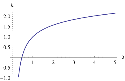
Figure 5: Entropy $\overline{h}[\mathfrak{G}_{\lambda}]$ for gamma laws

Finally for the third definition (22) of $\overline{h}$ we have the following values: for the Gaussian type we have

$$\overline{h}[\mathfrak{N}]=\ln\sqrt{2\pi e}\approx 1.41894$$ (51)

and for the uniform type

$$\overline{h}[\mathfrak{U}]=0$$ (52)

For the gamma types

$$\overline{h}[\mathfrak{G}_{\lambda}]=(1-\lambda)\psi(\lambda)+\ln\left[e^{\lambda}\Gamma(\lambda)\right]$$ (53)

the values, as displayed in the Figure 5, go from $-\infty$ for $\lambda\to 0^{+}$, to $+\infty$ for $\lambda\to+\infty$. In particular for the exponential type we have

$$\overline{h}[\mathfrak{E}]=1$$ (54)

For the Student types we finally have

$$\overline{h}[\mathfrak{T}_{\lambda}]=\frac{\lambda+1}{2}\left[\psi\left(\frac{\lambda+1}{2}\right)-\psi\left(\frac{\lambda}{2}\right)\right]+\ln\left[B\left(\frac{1}{2},\frac{\lambda}{2}\right)\right]$$ (55)

with values shown in the Figure 6 and going again from $+\infty$ at $\lambda\to 0^{+}$, to $-\infty$ for $\lambda\to+\infty$. In particular for the Cauchy type we get

$$\overline{h}[\mathfrak{C}]=\ln(4\pi)\approx 2.53102$$ (56)

As remarked in the Section 2.2, these examples show that the entropy $\overline{h}$ takes again all the (positive and negative) real values and hence that there is no maximum entropy distribution as in the case of the $\widetilde{h}$ entropy

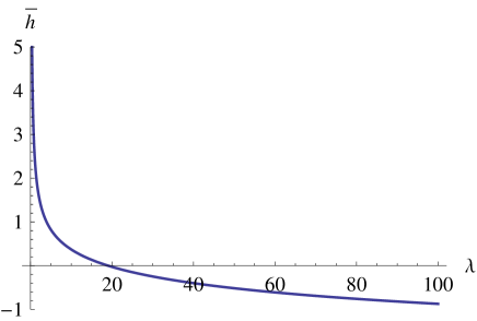
Figure 6: Entropy $\overline{h}[\mathfrak{T}_{\lambda}]$ for Student laws

Appendix B Mixtures

The definition of $\widetilde{\varrho}$ proposed in the Section 3 certainly produces non zero values for both purely discrete and purely continuous laws. Some care must be exercised however for discrete-continuous mixtures. Let us take for instance the mixture

$$\frac{2}{3}\,\bm{\delta}_{\frac{1}{2}}+\frac{1}{2}\,\mathfrak{U}(1)$$

of a law degenerate in $x=\frac{1}{2}$, and a law uniform in $[0,1]$. Its cdf would then be

$$F(x)=\left\{\begin{array}[]{ll}0&\quad x<0\\ \frac{2}{3}\,\vartheta\left(x-\frac{1}{2}\right)+\frac{x}{3}&\quad 0\leq x\leq 1\\ 1&\quad 1<x\end{array}\right.$$

where $\vartheta$ is the Heaviside function, and its quantile function is

$$Q(p)=\left\{\begin{array}[]{ll}3p&\quad 0\leq p\leq\frac{1}{6}\\ \frac{1}{2}&\quad\frac{1}{6}\leq p\leq\frac{5}{6}\\ 3p-2&\quad\frac{5}{6}\leq p\leq 1\end{array}\right.$$

as displayed in the Figure 7. It is apparent then that the IQrR is zero because

$$\varrho\left(\frac{1}{4}\right)=Q\left(\frac{3}{4}\right)-Q\left(\frac{1}{4}\right)=\frac{1}{2}-\frac{1}{2}=0$$

while the IQnR $\varrho(p)$ is a continuous function so that (with the notations of the Section 3) also $\widetilde{\varrho}=0$ because $\inf\mathcal{P}_{0}=0$. As a consequence, in the case of discrete-continuous mixtures with a cdf such as

$$F(x)=qF_{d}(x)+(1-q)F_{c}(x)\qquad\quad 0<q<1$$

we can not simply extend the definitions of the Section 3. We could however consider separately both the $\widetilde{\varrho}_{d}$ of the discrete distribution (as defined in the Section 3), and the $\widetilde{\varrho}_{c}=\varrho\left(\frac{1}{4}\right)$ of the continuous distribution, and to take as dimensional constant $\kappa$ their convex combination

$$q\,\widetilde{\varrho}_{d}+(1-q)\widetilde{\varrho}_{c}$$

which never vanishes because at least its continuous part is always non zero

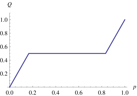
Figure 7: The quantile function $Q(p)$ for a mixture of degenerate and uniform laws

Acknowledgements

The author would like to thank A. Andrisani, S. De Martino, S. De Siena, C.J. Ellison and S. Stramaglia for invaluable comments and suggestions

References

- [1] M. Loève, Probability Theory I–II (Springer, Berlin, 1977-8).
- [2] P. Jacquet, W. Szpankowski, IEEE Trans. Inform. Th. 45 (1999) 1072
- [3] J. Cichoń, Z. Gołȩbiewski, DMTCS Proc. AQ (2012) 179, 23rd Intern. Meeting on Probabilistic, Combinatorial, and Asymptotic Methods for the Analysis of Algorithms (AofA’12)
- [4] T.M. Cover, J.M. Thomas, Elements of Information Theory, (Wiley, Hoboken, New Jersey, 2006)
- [5] L.M.A. Bettencourt, V. Gintautas, M.I. Ham, Phys. Rev. Lett. 100, 238701 (2008)
- [6] C. Tsallis, J. Stat. Phys. 52 (1988) 479
- [7] N. Drissi, T. Chonavel, J.M. Boucher, Res. Lett. Signal Proc. (2008) ID 790607