Maximum approximate entropy and r threshold: a new approach for regularity changes detection

Abstract

Approximate entropy (ApEn) has been widely used as an estimator of regularity in many scientific fields. It has proved to be a useful tool because of its ability to distinguish different system’s dynamics when there is only available short-length noisy data. Incorrect parameter selection (embedding dimension $m$, threshold $r$ and data length $N$) and the presence of noise in the signal can undermine the ApEn discrimination capacity. In this work we show that $r_{max}$ ($ApEn(m,r_{max},N)=ApEn_{max}$) can also be used as a feature to discern between dynamics. Moreover, the combined use of $ApEn_{max}$ and $r_{max}$ allows a better discrimination capacity to be accomplished, even in the presence of noise. We conducted our studies using real physiological time series and simulated signals corresponding to both low- and high-dimensional systems. When $ApEn_{max}$ is incapable of discerning between different dynamics because of the noise presence, our results suggest that $r_{max}$ provides additional information that can be useful for classification purposes. Based on cross-validation tests, we conclude that, for short length noisy signals, the joint use of $ApEn_{max}$ and $r_{max}$ can significantly decrease the misclassification rate of a linear classifier in comparison with their isolated use.

1 Introduction

The concept of changing complexity has proved to be helpful to characterize and assess different phenomena in areas such as seismology, economy, mechanics, physiology, etc. [1, 2, 3, 4]. In the last 30 years this challenging endeavor has led researchers and practitioners to develop different methods conceived to estimate and understand such complexity changes and their relationship with physical and biological system dynamics. In the early nineties, Lipsitz et al. reported that the process of natural aging is attached to a decrease of complexity in the dynamics of physiological functions [5]. This results in a loss in the capacity of the organism to adapt to stress, making it more vulnerable to diseases.

Approximate entropy finds its origins in Kolmogorov-Sinai Entropy (K-S Entropy), defined as the mean rate of information generated by a process [6, 7]. This measure is recognized for being a meaningful parameter to describe the behavior of dynamical systems. In [8] Grassberger and Procaccia provided an algorithm to calculate a lower bound for the K-S Entropy from a finite time series. Takens [9] and Eckmann and Ruelle [7] modified this approach to directly evaluate the K-S Entropy. Motivated by Eckmann-Ruelle Entropy, Pincus introduced the ApEn [10], providing a statistic to assess complexity from noisy short-length data. For an $N$-dimensional time series, ApEn depends on two parameters: the Embedding Dimension ($m$) and the Threshold ($r$). $ApEn(m,r)$ and $ApEn(m,r,N)$ can be seen respectively as a family of parametric statistics and estimators, designed to measure the regularity of a system. ApEn has been widely used as a non-linear feature to classify different dynamics, for example epileptic seizures [11, 12, 13] and sleep apnea [14].

Because of the bias introduced by counting self-matches and the finite data length ($N$), in [15, 16] the authors assert that the estimator $ApEn(m,r,N)$ lacks of consistency. To overcome this limitation, Richman et al. proposed the Sample Entropy (SampEn) as a more consistent regularity measure [16]. However, both ApEn and SampEn are highly dependent on the set of chosen parameters ($m$, $r$). Chon et al. [17] assert that neither ApEn nor SampEn is accurate in measuring the signal’s complexity when the calculations are made with the values of $m$ and $r$ recommended in the literature [18]. Instead, the use of $ApEn_{max}$, i.e. the maximum value of $ApEn(m,r,N)$, with fixed $m$ and $N$ was proposed as a more consistent estimator of system’s complexity [17, 19, 20].

The signal’s noise level has an important influence on $ApEn(m,r,N)$ estimation and therefore $ApEn_{max}$ is also affected. Pincus asserts that the reliability in the calculations could be seriously undermined when the Signal to Noise Ratio (SNR) is below 3 dB [18]. To overcome this issue, some authors have proposed a pre-processing step, in which, techniques such as Empirical Mode Decomposition (EMD) [21, 22] or Dyadic Wavelet Transform (DWT) [23] have been used.

In this paper, we will show that $r_{max}$ ($r$ value at which $ApEn(m,r,N)=ApEn_{max}$) brings useful information and can be also used as a feature for classification purposes. Furthermore, the use of $ApEn_{max}$ combined with $r_{max}$ can provide a more consistent method to discern between different dynamics even in presence of noise.

The remainder of this paper is organized as follows. In Section 2 we briefly recall the main approaches used for ApEn parameter selection and we present the methodology used in our simulations. In Section 3 the obtained results are summarized and discussed. Finally, in Section 4 the conclusions are presented.

2 Methods

In order to estimate $ApEn(r,m,N)$ for an $N$-dimensional time series $\left\{u_{1},u_{2},\dots,u_{N}\right\}$, given the parameters $m,~{}\tau~{}\in~{}\mathds{N}$, and $r\in\mathds{R^{+}}$, the $m$-dimensional embedded vectors $\boldsymbol{x}_{i}^{m}=\left[u_{i},u_{i+\tau},u_{i+2\tau},\dots,u_{i+(m-1)\tau}\right],$ with $1\leq i\leq N-(m-1)\tau,$ have to be considered. Then, the ApEn is defined as [10]:

$$\begin{array}[]{@{\hspace{-0.7cm}}l@{\hspace{2cm}}rcl}\hfil\hskip 56.9055pt&ApEn\left(m,r,N\right)&=&\phi^{m}\left(r\right)-\phi^{m+1}\left(r\right),\\ \text{where:}\hfil\hskip 56.9055pt&&&\\ \hfil\hskip 56.9055pt&\phi^{m}\left(r\right)&=&\frac{1}{N-(m-1)\tau}\sum\limits_{i=1}^{N-(m-1)\tau}{\ln{C_{i}^{m}\left(r\right)}},\\ \hfil\hskip 56.9055pt&C_{i}^{m}\left(r\right)&=&\frac{1}{N-(m-1)\tau}\sum\limits_{j=1}^{N-(m-1)\tau}{\theta\left(d\left(\boldsymbol{x}_{i}^{m},\boldsymbol{x}_{j}^{m}\right)-r\right)},\\ \hfil\hskip 56.9055pt&\theta\left(y\right)&=&\left\{\begin{array}[]{ll}0&\quad\text{if}\quad y>0,\\ 1&\quad\text{otherwise,}\end{array}\right.\\ \text{and}\hfil\hskip 56.9055pt&&&\\ \hfil\hskip 56.9055pt&d\left(\boldsymbol{x}_{i}^{m},\boldsymbol{x}_{j}^{m}\right)&=&\max\left\{\left|u_{i+k\tau}-u_{j+k\tau}\right|\right\},\qquad 0\leq k\leq m-1.\end{array}$$

The ApEn measures the logarithmic likelihood that two points ($\boldsymbol{x}_{i}^{m}$, $\boldsymbol{x}_{j}^{m}$) that are close (within a distance $r$) in an $m$-dimensional space, remain close in an $(m+1)$-dimensional space. Greater (lesser) likelihood of remaining close produces smaller (larger) ApEn values [24]. It is important to recall that $ApEn(m,r)$ was not conceived as an approximate value of E-R Entropy, therefore it cannot certify chaos. However, its scope relies on its ability to compare different types of dynamics [10]. Pincus asserts that, for a given system, ApEn values can vary significantly with $m$ and $r$ [18]. For this reason, it cannot be seen as an absolute measure. Moreover, this situation emphasizes the importance of the parameters’ selection to draw conclusions from ApEn estimations. In order to make this paper self contained, we will review some results for parameter selection.

2.1 Embedding dimension ($m$)

The main purpose of embedding a time series is to unfold the projection to a state space that is representative of the original system’s space, i.e. a reconstructed attractor must preserve the invariant characteristics of the original one [25]. Takens’ embedding theorem gives sufficient conditions to accomplish this task using any $m$ bigger than twice the Hausdorff dimension of the chaotic attractor. The idea is to estimate the minimum embedding dimension since a bigger $m$ will lead to excessive computational efforts. Kennel et al. proposed a parametric algorithm to determine the minimum embedding dimension, named False Nearest Neighbors [26]. Its main disadvantage is that the results highly depend on the choice of the algorithm parameters. A slightly different approach was proposed by Cao [27]. This method does not rely upon subjective parameters other than the embedding lag.

Pincus has suggested to set $m=2$ or $m=3$ [15, 18]. That advice arises from the fact that, once $N$ is set, high $m$ values conduct to poor $ApEn(m,r)$ estimations. This is due to the bias introduced by self-counting and the decreased number of vectors $\boldsymbol{x}_{i}^{m}$ available to estimate $C_{i}^{m}\left(r\right)$. The aforementioned approach may be convenient when low-dimensional systems are studied. However, when the dimension is high, this criterion will lead to a poor reconstruction of the process’ dynamics [28, 29], causing inconsistencies in presence of noise.

It is worthwhile noting that typical applications with ApEn have been conducted using the previously mentioned values of $m$. Aletti et al. set $m=2$ to assess congenital heart malformation in children using Heart Rate Variability (HRV) signals [30]. Zarjam et al. use $m=2$ and $3$ to calculate $ApEn(m,r)$ from electroencephalogram (EEG) signals to investigate changes in working memory load during the performance of a cognitive task with varying difficulty levels [31].

2.2 Embedding Lag ($\tau$)

The objective of selecting $\tau$ is to maximally spread the data in the phase space, removing redundancies and making fine features more easily discernible [29]. In most ApEn applications $\tau$ is set to one. Kaffashi et al. [32] concluded that, for time series generated by non-linear dynamics and whose Autocorrelation Function decays rapidly, $\tau=1$ is sufficient to provide a good estimation of signal complexity. However, for signals with long range correlation, a $\tau$ equal to time occurrence of the first local minimum of the Mutual Information Function or to the time occurrence of the first zero crossing of the Autocorrelation Function can provide additional information [29, 32].

2.3 Threshold (r)

As it was aforementioned, the statistics $ApEn(m,r)$ can vary significantly with $r$. Pincus suggests that $r$ should lie between $0.1-0.2$ times the standard deviation (SD) of the raw signal [33, 34]. The $r$ value should be large enough, not only to avoid significant contribution from noise, but also to admit a reasonable number of $\boldsymbol{x}_{i}^{m}$ vectors being within a distance $r$. This would ensure an acceptable estimation of the $C_{i}^{m}\left(r\right)$ probability [18]. However, with too large $r$ values, $ApEn(m,r)$ is unable to perform fine process distinctions and consequently, the $r$ value selection will greatly depend on the application [15].

Although the later approach has been broadly applied [35, 36, 37], some authors assert that sometimes this methodology leads to an incorrect assessment of complexity [17, 19, 20]. They proposed the use of $ApEn_{max}$ as a better complexity estimator. One main issue arises from the fact that the calculation of $ApEn_{max}$ requires high computational efforts. To overcome this limitation, a set of equations was proposed to calculate a parameter $\hat{r}_{max}$ as an approximation to $r_{max}$ [17, 20]. Supported on experimental results with HRV signals, Castiglioni et al. concluded that the use of $ApEn_{max}$ seems to be a reasonable approach, because this choice would allow the time series complexity to be better quantified than any other choice of $r$ [38]. On the other hand, Liu et al. observed that $ApEn_{max}$ was incapable of distinguishing between groups of healthy and heart failure subjects, in experiments with HRV signals. Further, since they found that $\hat{r}_{max}$ fails in estimating $r_{max}$ for the Logistic map, they asserted that care must be taken when using $\hat{r}_{max}$ [39]. In a recent study, Boskovic et al. [40], present some evidence of $ApEn_{max}$ instability. They observed that for two time series, the estimated $ApEn_{max}$ value suggests opposite results when data length decreases. There are other algorithms conceived to reduce the computational effort of calculating the whole profile of ApEn as a function of $m$ and $r$ [41, 42].

Model	Equation	Model Parameters	ApEn Parameters
Mackey-Glass	$\displaystyle{dx}/{dt}$ $\displaystyle=bx+(a\tilde{x})/(1+\tilde{x}^{c})$ $\displaystyle\tilde{x}$ $\displaystyle=x(t-\Delta)$	$\displaystyle c$ $\displaystyle=\left\{4.5,\,6\right\}$ $\displaystyle a$ $\displaystyle=0.9$ $\displaystyle b$ $\displaystyle=0.3$ $\displaystyle\Delta$ $\displaystyle=80$ $\displaystyle\Delta t$ $\displaystyle=1$	$\displaystyle m$ $\displaystyle=\left\{2,\,\,3,\dots,20\right\}$ $\displaystyle r$ $\displaystyle=\left\{0,\,\,5\times 10^{-5},\dots,0.035\right\}$ $\displaystyle\tau$ $\displaystyle=83$ $\displaystyle N$ $\displaystyle=5000$
Shilnikov’s type	$\displaystyle{dx}/{dt}$ $\displaystyle=y$ $\displaystyle{dy}/{dt}$ $\displaystyle=z$ $\displaystyle{dz}/{dt}$ $\displaystyle=\mu x-y-\varepsilon z-ax^{2}-bx^{3}$	$\displaystyle a$ $\displaystyle=\left\{0.008,\,\,0.2217\right\}$ $\displaystyle\varepsilon$ $\displaystyle=0.55$ $\displaystyle\mu$ $\displaystyle=0.65$ $\displaystyle b$ $\displaystyle=0.65$ $\displaystyle\Delta t$ $\displaystyle=0.2$	$\displaystyle m$ $\displaystyle=\left\{2,\,\,3,\dots,20\right\}$ $\displaystyle r$ $\displaystyle=\left\{0,\,\,5\times 10^{-5},\dots,0.035\right\}$ $\displaystyle\tau$ $\displaystyle=10$ $\displaystyle N$ $\displaystyle=5000$

Table 1: Simulation models and parameters. $\Delta t$ stands for the time step used to obtain the numerical solutions. The upper bound of the $r$ range is equal to the SD of the normalized signal.

2.4 Simulations

In the presence of noise, the estimator $ApEn_{max}$ could be incapable to discern between different dynamics. Here we address the hypothesis that $r_{max}$ provides additional information valuable for the discrimination process. In other words, the use of both $ApEn_{max}$ and $r_{max}$ would increase the ability of discerning between different complexities in the case of noisy time series. To assess this hypothesis four simulations were conducted: three of them with synthetic signals and the last one with an EEG record.

As a first case the Mackey-Glass delay-differential equation was used [27]. Our aim is to assess these estimators on time series from a high-dimensional system [43]. This system have been used not only to study the behavior of complexity estimators on high-dimensions [8] but also to model the dynamics of physiological control systems like the neurological system [43], the respiratory system [44] and the hematopoietic system [44].

Two sets of $240$ realizations were produced for each value of the $c$ parameter (see Table 1). Each realization with $25000$ points has a different initial condition, randomly chosen from a $\mathcal{U}(0,0.01)$ distribution. In order to avoid the influence of transients, the first $20000$ points of each realization were discarded. The resulting signals (with length $N=5000$) were normalized to have unitary energy. For two randomly selected signals, one from each set, its Mutual Information Function was calculated. Then, the lag corresponding to each first local minimum was selected, and the $\tau$ parameter was fixed as the largest between these values. $ApEn(m,r,N)$ was calculated for each signal, with $m$ and $r$ taking the values listed in Table 1 and $ApEn_{max}$ and $r_{max}$ were found from the $ApEn(m,r,N)$ functions. Additionally an estimator of the minimum embedding dimension was calculated for all signals using Cao’s algorithm [27].

With the goal of analyzing synthetic data from a system that resembles a particular physiological dynamics, a Shilnikov’s type chaos model was considered as a second case. The same methodology as in the first case was adopted for Shilnikov’s type model using two values of the $a$ parameter (see Table 1), which allow simulating EEG signals recorded during a seizure of petit mal epilepsy [45]. The initial conditions for each realization were selected from a $\mathcal{U}(0,0.01)$ distribution and the $x$ variable was used for the calculations.

In order to evaluate our method in presence of noise, white Gaussian noise was added to each signal (Mackey-Glass and Shilnikov) with SNR$=5$ dB and SNR$=0$ dB. Then, all realizations were normalized to have unitary energy and both $ApEn_{max}$ and $r_{max}$ were calculated as previously described. Table 1 summarizes the models and the parameter values used to obtain the time series as well as the parameter values used to calculate the ApEn.

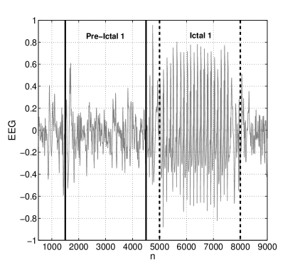
(a)

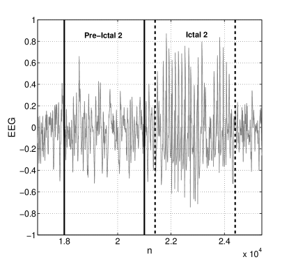
(b)

Fig. 1: EEG signal: (a) First pre-ictal and ictal episodes. (b) Second pre-ictal and ictal episodes.

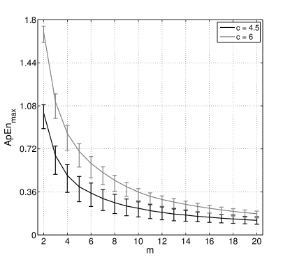
(a)

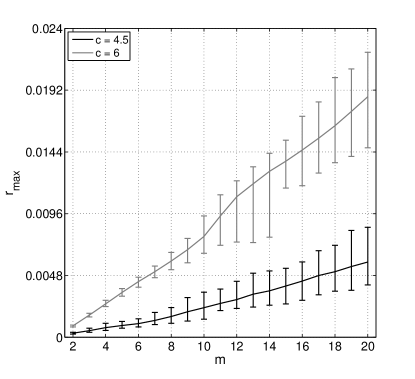
(b)

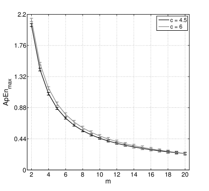
(c)

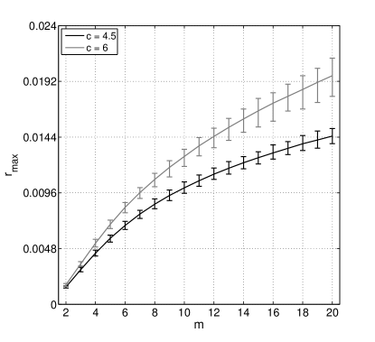
(d)

Fig. 2: Mackey-Glass model: mean and $95\%$ confidence interval. Noiseless: (a) $ApEn_{max}$. (b) $r_{max}$. With SNR$=5$ dB: (c) $ApEn_{max}$. (d) $r_{max}$.

A real physiological signal recorded using stereo electroencephalography (EEG) with eight multilead electrodes (2 mm long and 1.5 mm apart) was studied. It was filtered and amplified using a 1-40 Hz band-pass filter. A four-pole Butterworth filter was used as anti-aliasing low-pass filter. This signal was digitized at 256 Hz through a 10 bits A/D converter. A physician accomplished the analysis of pre-ictal and ictal data by visual inspection of the EEG record. According to the visual assessment of the EEG seizure recording, the patient presented an epileptogenic area in the hippocampus with immediate propagation to the girus cingular and the supplementary motor area, on the left hemisphere. In Fig. 1, the EEG signal of two ictal and two pre-ictal episodes corresponding to a depth electrode in the hippocampus is presented. All these episodes contains 3000 data samples. The first pre-ictal and ictal episodes comprise the signal portions for $n\in[1500,4500]$ and $n\in[5000,8000]$ data points respectively. The second pre-ictal and ictal portions were selected for $n\in[18000,21000]$ and $n\in[21400,24400]$ respectively. Each of the data sets were normalized to have unitary energy and the $\tau$ parameter was selected as described above among the four signals. $ApEn_{max}$ and $r_{max}$ were then calculated for $2\leq m\leq 20$. Additionally, white Gaussian noise was added to the raw EEG signal with SNR$=5$  dB (the actual SNR of the EEG signal is unknown) and $ApEn_{max}$ and $r_{max}$ were calculated again.

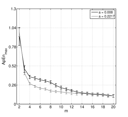
(a)

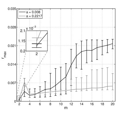
(b)

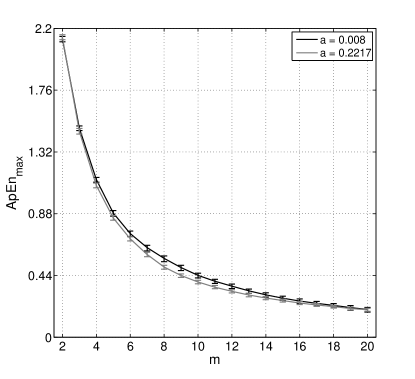
(c)

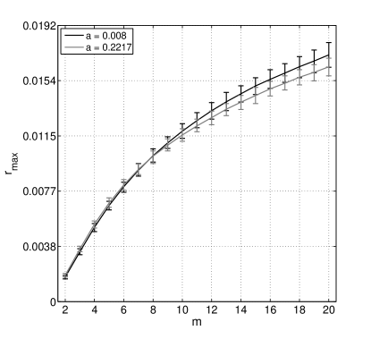
(d)

Fig. 3: Shilnikov’s type chaos model: mean and $95\%$ confidence interval. Noiseless: (a) $ApEn_{max}$. (b) $r_{max}$. With SNR$=5$ dB: (c) $ApEn_{max}$. (d) $r_{max}$. In (b) an enlarged view for $m=2$ is presented.

3 Results and Discussion

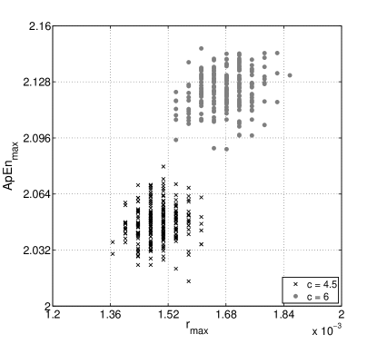
(a)

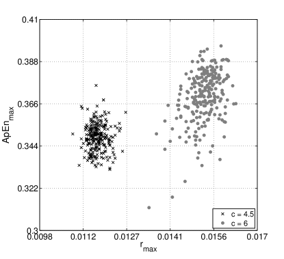
(b)

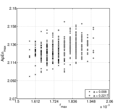
(c)

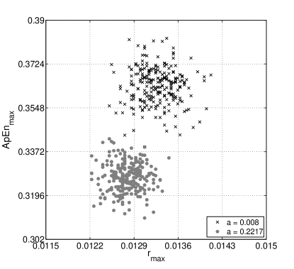
(d)

Fig. 4: SNR$=5$ dB, $ApEn_{max}$ vs $r_{max}$ plot: (a) Mackey-Glass model $m=2$. (b) Mackey-Glass model $m=12$. (c) Shilnikov’s type model $m=2$. (d) Shilnikov’s type model $m=12$.

Fig. 2 summarizes the results obtained for the Mackey-Glass model simulations. The $ApEn_{max}$ and $r_{max}$ mean and $95\%$ confidence interval (CI) are presented as functions of $m$ for two different $c$ parameter values. The CIs were empirically obtained by sorting the $ApEn_{max}$ and $r_{max}$ values calculated from the $240$ realizations and taking the $2.5\%$ and the $97.5\%$ quantiles as the lower and upper bound respectively. In Fig. 2a, it can be noticed that the curves of $ApEn_{max}$ become closer as $m$ increases, achieving the maximum distance at $m=2$. On the contrary, in Fig. 2b it can be observed that the distance between the $r_{max}$ curves becomes larger as $m$ increases. Figs. 2c and 2d show the effect of noise over $ApEn_{max}$ and $r_{max}$ estimations. First, notice that, compared to noise free figures, the mean values of $ApE_{max}$ and $r_{max}$ are increased due to the addition of noise. Additionally, in both cases, the CIs are reduced. Finally, the $ApEn_{max}$ and $r_{max}$ curves for different $c$ parameter values are closer to each other than in the case without noise. It is important to remark that, in presence of noise, while $r_{max}$ is still able to discern between dynamics, the discrimination capacity of $ApEn_{max}$ is highly reduced. In conclusion, these results suggest that $r_{max}$ can bring useful information even in presence of noise.

Shilnikov’s type chaos model results are presented in Fig. 3. In Fig. 3a, it can be noticed that it is impossible to distinguish the two dynamics using $ApEn_{max}$ calculated with $m=2$. Nevertheless, embedding the system in a higher dimension such as $m=3$ (minimum embedding dimension), distinctions between dynamics can be made. However, in Fig. 3b, it can be seen that for $m=2$, $r_{max}$ indicates a difference between dynamics. The added noise has the same above mentioned influence over both $ApEn_{max}$ and $r_{max}$ (see Figs. 3c and 3d). However, in this case the $r_{max}$ curves are closer than those corresponding to the Mackey-Glass system. From this simulation we can conclude that using $ApEn_{max}$ or $r_{max}$ independently can be inconvenient for classification purposes. Instead, we propose to study the combined use of both estimators for this task.

In order to illustrate the advantages of this new approach, Fig. 4 shows scatter plots of $ApEn_{max}$ vs $r_{max}$ for both models with noise (SNR$=5$ dB), using $m=2$ and $m=12$. In the presence of noise, it is enough to set $m=2$ and to use only $ApEn_{max}$ to correctly differentiate the two dynamics from the Mackey-Glass model (see Fig. 2c). However, in Fig. 4a it can be noticed that $r_{max}$ provides additional information that can make easier the classification process. A slightly different situation can be appreciated for Shilnikov’s type dynamics. Fig. 4c shows that it is not possible to discern between classes using $ApEn_{max}$ calculated with $m=2$. Nevertheless, with the information brought by $r_{max}$, the two classes can be separated in a more suitable way. As presented before, when there is noise in the signal, the assessment of $ApEn_{max}$ using an $m$ value equal or larger than the minimum embedding dimension could be more accurate and robust than just setting $m=2$. Cao’s algorithm suggests that the minimum embedding dimension for both models should be $m\approx 12$. Such large $m$ value is the result of noise influence in the estimation of the systems’ minimum embedding dimension. The issue is that, for the Mackey-Glass model, $ApEn_{max}$ losses its discrimination capacity for high $m$ values. Nonetheless, as can be appreciated in Fig. 4b, the two classes can be still successfully separated using only $r_{max}$. On the other hand, Fig. 4d shows that for $m=12$, the two different dynamics from the Shilnikov’s type model can be more conveniently clustered using $ApEn_{max}$ than using $r_{max}$. These results remark the importance of using both estimators together instead of each one individually.

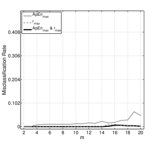
(a)

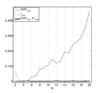
(b)

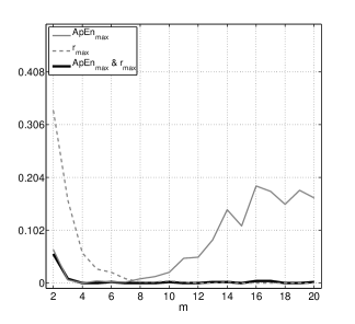
(c)

(d)

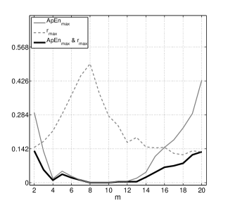
(e)

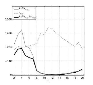
(f)

(g)

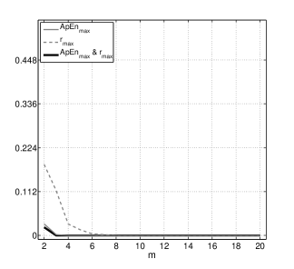
(h)

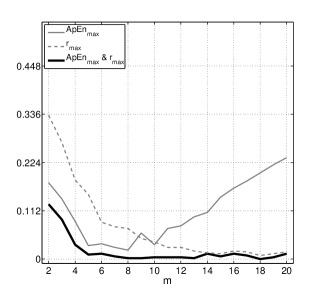
(i)

Fig. 5: 10-fold cross-validation misclassification rate with a linear SVM classifier. Mackey-Glass model: (a) noiseless. (b) SNR$=5$ dB. (c) SNR$=0$ dB. Shilnikov’s type model: (d) noiseless. (e) SNR$=5$ dB. (f) SNR$=0$ dB. Logistic map: (g) noiseless. (h) SNR$=5$ dB. (i) SNR$=0$ dB.

In addition to the Mackey-Glass and Shilnikov’s systems we introduce calculations of $ApEn_{max}$ and $r_{max}$ using dynamics from the Logistic map, $x_{n+1}=Rx_{n}(1-x_{n})$, in two chaotic regimes ($R=3.75$, $R=3.95$) with and without white Gaussian noise. $ApEn_{max}$ and $r_{max}$ were evaluated using the procedure aforementioned for $2\leq m\leq 20$ with $\tau=1$ and $N=5000$.

With the goal of quantitatively verifying the proficiency of $ApEn_{max}$ and $r_{max}$ as classification features, we perform a 10-fold cross-validation using linear support vector machines (SVMs). We choose a linear classifier given that its simplicity will disclose the real quality of the features. The basic idea behind the SVMs is to separate the classes using the optimal hyperplane (the linear decision function that maximizes the distance between the closest points of different classes to the hyperplane) [46]. In Fig. 5 the Misclassification Rates (MR) for three classifiers as functions of $m$ and different noise levels (noiseless, SNR$=5$ dB and SNR$=0$ dB) are presented. The first classifier uses only $ApEn_{max}$ as input feature, the second one uses only $r_{max}$, and the third one uses jointly both estimators.

For the noiseless Mackey-Glass system, it can be seen in Fig. 5a that the MR of the first classifier increases with $m$, achieving its maximum ($0.065$) for $m=19$. Further, the second classifier presents a non-zero MR only for $m\geq 15$. The MR for the third classifier is zero for $0\leq m\leq 14$ with a maximum value of $0.006$ at $m=15$. A similar behavior can be observed for the Mackey-Glass model immersed in noise (SNR$=5$ dB). In contrast with the noiseless case, in Fig. 5b it is shown that the MR of the classifier which uses only $ApEn_{max}$ has been greatly increased. Additionally, using only $r_{max}$, the classifier has non-zero MR for $2\leq m\leq 4$. Nevertheless, the MR of the classifier that uses both estimators still remains equal to zero for $2\leq m\leq 4$ values. For the case in which the SNR$=0$ dB (Fig. 5c), it can be noticed that the MR of the third classifier is always below or equal to the lowest MR between the other two classifiers. The last results attest that, as an ensemble, $ApEn_{max}$ and $r_{max}$ provide features that are robust against noise.

Regarding the results for the noiseless Shilnikov’s model, it is shown in Fig. 5d that, for $3\leq m\leq 11$ the MR of the first classifier is lower than the second classifier’s MR. For $m=2$ as well as for $12\leq m\leq 20$, the last statement is reversed. However, the MR for the third classifier remains below the MR of the other two ones, being zero for $4\leq m\leq 11$ and for $16\leq m\leq 20$. Additionally, from Fig. 5e it can be noticed that for all $m$ values the MR of the third classifier is always below or equal to the lowest MR value between the other two classifiers, being zero for $8\leq m\leq 10$ and $0.004$ for $m=12$. For the SNR$=0$ dB case, it can be observed in Fig. 5f that for $m\geq 8$ very low MR values are achieved by the first and third classifiers, being zero for $10\leq m\leq 15$.

Very similar results were achieved with the logistic map (Figs. 5g, 5h, 5i). The MR of the classifier that uses in conjunction $ApEn_{max}$ and $r_{max}$ is zero for all $m$ values in the noiseless case and for $m\geq 3$ in the SNR=$5$ dB case. From Fig. 5i it can be seen that the MR of the third classifier is below the MR of the other classifiers for all $m$ values, being zero for $m=8$ and $m=9$ and achieves a very low value for $m\geq 5$. This results lead us to think about the usefulness of these estimators to discriminate dynamics from discrete-time non-linear systems.

It is important to notice that when these three systems were immersed in high levels of noise (see Figs. 5c, 5f and 5i) the worst results were achieved for low $m$ values (specially for $m=2$). This suggests that increasing the embedding dimension could be beneficial for the discrimination process. As a conclusion, these results highlight the complementary relationship between both estimators and the benefits of being used together. It is also important to observe that the use of both estimators enlarges the range of $m$ values that can be selected to achieve a good classification performance in presence of noise. Nonetheless, using an estimate of the minimum embedding dimension can be a wise choice (see Fig. 5c and 5f for $m=12$).

There is an interesting fact in these results concerning the presence of noise in the time series. As it was discussed before, the addition of noise not only decreases the distance of $ApEn_{max}$ and $r_{max}$ curves between different dynamics but it also reduces both estimators’ CI. The trade-off between these two phenomena is more evident as the SNR is reduced. In Figs. 5b and  5c, it can be seen that for $m\geq 4$ the MR of the first classifier is larger for SNR$=5$ dB than for SNR$=0$ dB. As a consequence of this trade-off, the distributions of $ApEn_{max}$ values for two different dynamics are more overlapped in the case with SNR$=5$ dB than when SNR$=0$ dB. The last statement can be verified comparing the Bhattacharyya coefficient ($B_{c}$) [47] between the $ApEn_{max}$ distributions of different dynamics for different SNRs. For two density functions $p$ and $q$ over the same domain $X$, this coefficient is defined as $B_{c}\left(p,q\right)=\sum_{x\in X}\sqrt{p(x)q(x)}$, $0\leq B_{c}\leq 1$, being zero if $p(x)$ and $q(x)$ do not overlap. The $B_{c}$ coefficients between $ApEn_{max}$ distributions ($m=19$) for SNR$=5$ dB and SNR=$0$ dB are $0.91$ and $0.53$ respectively. This fact explains why the MR of this classifier is lower for SNR$=0$ dB than for SNR$=5$ dB when high $m$ values are used with systems like Mackey-Glass and Shilnikov’s.

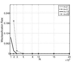
(a)

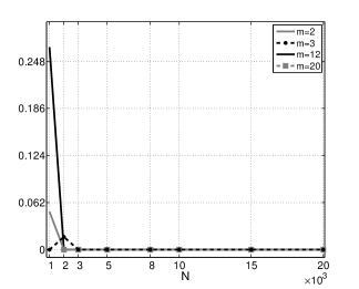
(b)

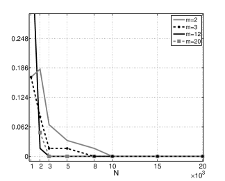
(c)

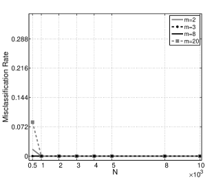
(d)

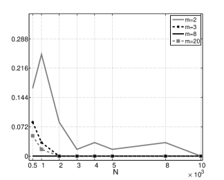
(e)

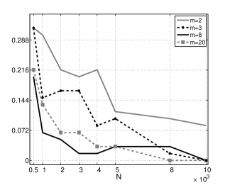
(f)

Fig. 6: Misclassification rate as a function of the data length. Mackey-Glass model: (a) noiseless. (b) SNR$=5$ dB. (c) SNR$=0$ dB. Logistic map: (d) noiseless. (e) SNR$=5$ dB. (f) SNR$=0$ dB.

An important topic that must be considered in the calculation of $ApEn_{max}$ and $r_{max}$ is the data length. When the time series is short, the choice of large $m$ and $\tau$ values can be harmful because the estimation of conditional probabilities becomes unreliable [10, 15]. However, there is another issue that can alter their estimation and it is related to the use of small $m$ values.

It is known that poor state space reconstructions are obtained when the system is embedded with an $m$ value smaller than the system’s minimum embedding dimension, and such situation brings to the occurrence of false neighbors [28], i.e. points that are close due to a low embedding dimension rather than because of the system’s dynamics. Given that the estimation of conditional probabilities is based on counting neighbors’ occurrences, an appropriate selection of the $m$ value demands to take into account an estimation of the minimum embedding dimension [29]. With the aim of assess the behavior of our method as a function of the data length, the next simulation was conducted over the Logistic map and the Mackey-Glass system.

Two sets of $30$ realizations were built. Each set was obtained using a different value of the $R$ parameter for the Logistic map and, of the $c$ parameter for the Mackey-Glass system. Each signal of these sets was normalized to have unitary energy. For the Logistic map $ApEn_{max}$ and $r_{max}$ were estimated with $m=\left[2,3,8,20\right]$, $\tau=1$ and $N=\left[0.5,1,2,3,4,5,8,10\right]\times 10^{3}$. For the Mackey-Glass system these estimators were evaluated with $m=\left[2,3,12,20\right]$, $\tau=83$ and $N=\left[1,2,3,5,8,10,15,20\right]\times 10^{3}$. Then, the misclassification rate of a linear SVM classifier that uses both estimators as features was computed using Leave one Out cross-validation. Additionally, the same procedure was used over the same signals contaminated with white Gaussian additive noise (SNR$=5$ dB and SNR$=0$ dB). It is important to mention that the values of $m=8$ and $m=12$ were suggested by the Cao’s algorithm [27] as minimum embedding dimensions for the noisy signals (SNR$=0$ dB) from the Logistic map and, from the Mackey-Glass system respectively. For the Mackey-Glass system the calculations with $m=20$ were made for all $N$ values except $N=1000$.

In Fig. 6 it is shown the misclassification rate calculated for both systems as a function of $N$ and the noise level. In Fig. 6a are shown the results for the noise free Mackey-Glass system. It can be observed that for small data length values the biggest errors are achieved using $m=20$ ($N=2000$) and $m=12$ ($N=1000$); this is a consequence of the reduced amount of information available to estimate the conditional probabilities. Nevertheless, as $N$ is increased, the error for all $m$ values goes to zero. It must be noticed that for $m=2$ and $m=3$ the error is zero for all $N$ values.

On the other hand Fig. 6b shows that, compared with the noiseless case, for $m=2$ (at $N=1000$) and $m=3$ (at $N=2000$) the error has increased its value from zero, whereas the error for $m=12$ and $m=20$ has decreased its values to zero for $N=2000$. Observe that the error is zero from $N\geq 3000$ regardless the value of $m$. From Fig. 6c it can be seen that, excluding the error (equal to $0.48$) for $m=12$ at $N=1000$, the biggest error is accomplished using $m=2$ followed by the one obtained with $m=3$ for $1000\leq N\leq 8000$. However, the error for $m=12$ and $m=20$ is always lesser or equal to the error achieved with $m=2$ or $m=3$, moreover, it is zero starting from $N=3000$. Comparing Figs. 6a and 6c for m = 2 and m = 3 it is clear that, for small $N$ values, a poor state space reconstruction added to the presence of noise deteriorates the discrimination capacity of $ApEn_{max}$ and $r_{max}$.

For the noiseless Logistic map (Fig. 6d) it can be observed that for $N=500$ the biggest error ($0.08$) belongs to the estimators calculated with $m=20$ followed by the error calculated with $m=2$ ($0.017$). However, for $m=3$ and $m=8$ the error is zero. Moreover, as $N$ is increased, the error remains equal to zero for all $m$ values. It can be seen Fig. 6e that the biggest error is achieved with $m=2$ for all $N$ values except $N=10000$. Instead, for $m=8$ the error is equal to zero for all $N$ values. It is worth mentioning that for all $N$ values the error obtained with $m=8$ and $m=20$ is always below or equal to the error attain with $m=2$ and $m=3$. From Fig. 6f it can be noticed that using $m=2$ produces the worst classification error regardless the value of $N$ and the best results are accomplished using $m=8$ and $m=20$ for almost all $N$ values.

Based on these results we can conclude that in the $ApEn_{max}$ and $r_{max}$ estimation’s processes it is highly recommended to keep in mind that there exists a trade-off between $m$ and $N$, and special attention is needed in the presence of noise. When data length is short and there is not noise in the signal, relative small $m$ values provides the best performance. However, in presence of noise, it would be wise either to use an estimation of the system’s minimum embedding dimension whenever it is possible, or to use a value as close as possible to it when the data length is a limitation. It must also be considered that in real applications, such as epileptic seizures’ detection, the duration of some events is only of a few samples: for example absence seizures often last less than $5$ seconds [48], which correspond to $1280$ samples using a standard sampling frequency of $256$ Hz. Although for small $N$ values there is no guarantee of an accurate estimation of $ApEn_{max}$ nor $r_{max}$ with relative high $m$ values. The results here presented show that using $m$ values above $2$ or $3$ can increase the discrimination capacity of these estimators, specially in presence of noise.

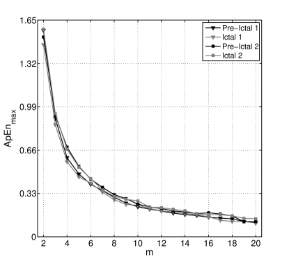
(a)

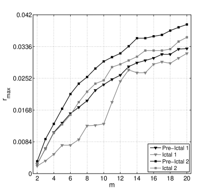
(b)

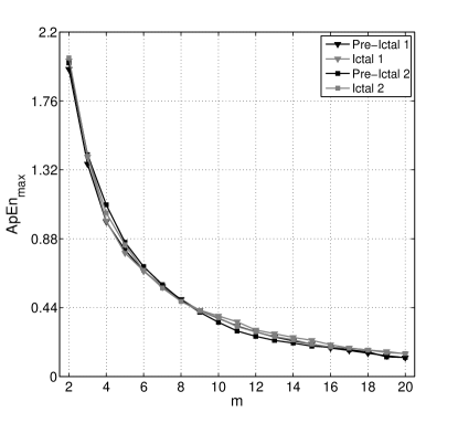
(c)

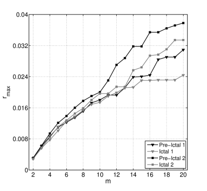
(d)

Fig. 7: EEG signal. Two ictal episodes and their respective pre-ictal segments. Raw signal: (a) $ApEn_{max}$. (b) $r_{max}$. SNR$=5$ dB: (c) $ApEn_{max}$. (d) $r_{max}$.

The studies conducted on the EEG recording provided similar results to those obtained with the previous simulations. In Fig. 7 are presented the $ApEn_{max}$ and $r_{max}$ curves as functions of $m$ for two ictal episodes and their respective pre-ictal segments. The distances (relative to the scale) between the $ApEn_{max}$ curves of each ictal and its corresponding pre-ictal episodes are small for all the $m$ values, as can be observed in Fig. 7a. On the contrary, Fig. 7b suggests that $r_{max}$ can be used to discriminate between dynamics. Decreasing the SNR tends to reduce the distance between $ApEn_{max}$ and $r_{max}$ curves (see Figs. 7c and 7d). However, for high $m$ values, the information given by $r_{max}$ can be useful to distinguish between dynamics.

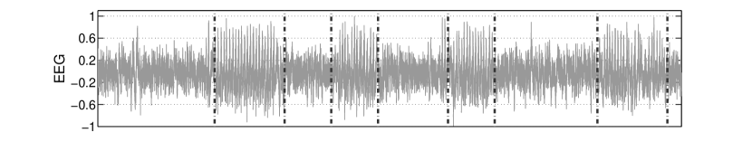
(a)

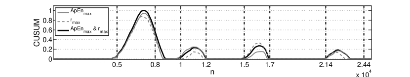
(b)

Fig. 8: Ictal episodes detection using $ApEn_{max}$ and $r_{max}$ from an EEG signal with additive noise (SNR$=5$ dB): (a) EEG signal. (b) CUSUM over the first PC on the $\boldsymbol{C^{A}}$, $\boldsymbol{C^{R}}$ and $\boldsymbol{C^{AR}}$ matrices. The ictal episodes can be found between vertical dashed lines.

It is worth mentioning that, for this signal and with these estimators, it is difficult to separate the ictal and pre-ictal episodes as isolated groups. However, it is possible to state differences between an ictal episode and its corresponding pre-ictal one. This result leads us to think that a suitable approach to detect ictal episodes from EEG signals, using these estimators, should be one in which their temporal evolution could be evaluated.

In order to assess this idea, we corrupted the EEG signal with white Gaussian noise (SNR$=5$ dB) and we considered sliding windows of length $N=1000$, shifted $128$ data points. Each window was normalized to have unitary energy. $ApEn_{max}$ and $r_{max}$ were estimated using $\tau=10$ for $2\leq m\leq 6$. With these results we proceed as follows: first, we built the matrices $\boldsymbol{C^{A}}$ and $\boldsymbol{C^{R}}$, where the entry $C^{A}_{k,i}$ was the value of $ApEn_{max}$ calculated with the i-th value of $m$ for the k-th window. The matrix $\boldsymbol{C^{R}}$ was built alike with the $r_{max}$ values. Each matrix was statistically normalized (zero mean and unitary SD) by columns. Observe that the temporal evolution of $ApEn_{max}$ and $r_{max}$ calculated with the i-th $m$ value can be evaluated by looking the i-th column of the $\boldsymbol{C^{A}}$ and $\boldsymbol{C^{R}}$ matrices respectively. A third matrix named $\boldsymbol{C^{AR}}$ was conformed by the horizontal concatenation of the above mentioned matrices: $\boldsymbol{C^{AR}}=\left(\boldsymbol{C^{A}}\,|\,\boldsymbol{C^{R}}\right)$. Next, we performed a Principal Component Analysis (PCA) over each matrix. The first principal component ($1^{st}$PC) can be thought as a summary that best represents the information collected by these estimators through all $m$ values. Finally, an algorithm for detection of abrupt mean changes (CUSUM) was applied on the $1^{st}$PC of each matrix [49]. The target mean and the reference value were fixed as the average of the first twenty data points and two times their SD, respectively.

In Fig. 8 are presented the EEG signal with the four ictal episodes marked between vertical dashed lines (Fig. 8a) and the results of the CUSUM algorithm applied over the $1^{st}$PC of each matrix (Fig. 8b). It can be observed in Fig. 8b that all ictal episodes can be detected using the information contained in each matrix. Nevertheless, while some ictal episodes are better detected with $ApEn_{max}$, others are better detected with $r_{max}$. On the other hand, a more consistent identification of ictal episodes can be achieved using in conjunction both estimators. These results suggest that, with the information provided by both $ApEn_{max}$ and $r_{max}$ for different $m$ values, the ability to discriminate between different dynamics can be increased (even in presence of noise), since changes that cannot be identified in the temporal evolution of one estimator could be identified in the temporal evolution of the other one. It must be remarked that these findings only suggest the suitability to jointly use both estimators to detect ictal episodes from EEG signals. Further experiments with a large data base will be conducted in future works to statistically assess the performance of the proposed method to detect complexity changes in real signals.

4 Conclusions

The approximate entropy has been recognized by its ability to distinguish between different system’s dynamics when short-length data with moderate noise are available. However, it is also known that high noise levels and incorrect parameter selection can undermine its discrimination capacity. In order to overcome these difficulties, in this paper we have proposed a method based on the use of $r_{max}$ along with $ApEn_{max}$ to discern between different dynamics. Using signals from real physiological and from simulated low- and high-dimensional systems, with and without noise, we have studied the behavior of $ApEn_{max}$ and $r_{max}$ as functions of the embedding dimension, the data length and the noise level. The results indicate that, even in presence of noise, $r_{max}$ provides valuable information that can be used for classification purposes. Furthermore, as these estimators vary with $m$, there is a complementary relationship between them, which strengthens the idea of using $ApEn_{max}$ combined with $r_{max}$ to distinguish between dynamics. Cross-validation simulations have demonstrated that the jointly use of both estimators as input features, significantly decreases the misclassification rate of a simple linear classifier. Moreover, the conjoint use of both estimators enlarges the range of $m$ values that can be chosen to achieve a good classification performance. Concerning the data length, we have shown that for short-length signals good discriminating features can be achieved using relative small $m$ values if there is no noise. However, in presence of noise the discrimination capacity of $ApEn_{max}$ and $r_{max}$ can be increased using $m$ values above $2$ or $3$. Our results encourage the use of an estimation of the system’s minimum embedding dimension when it is possible, or the use of a close enough value when the data length is a limitation. We assert that as well as $ApEn_{max}$, the estimator $r_{max}$ can also be utilized to discern between dynamics even in the presence of noise. Moreover, the use of $r_{max}$ has shown to be helpful in such cases when $ApEn_{max}$ is unable to contrast between processes that are immersed in noise. The link between $r_{max}$ and system complexity will be addressed in future studies, to reveal the nature of this relationship and its physical meaning.

References

- [1] S. M. Potirakis, G. Minadakis, K. Eftaxias, Analysis of electromagnetic pre-seismic emissions using Fisher information and Tsallis entropy, Physica A: Statistical Mechanics and its Applications 391 (1) (2012) 300–306.
- [2] F. Isik, An entropy-based approach for measuring complexity in supply chains, International Journal of Production Research 48 (12) (2010) 3681–3696.
- [3] Y. He, J. Huang, B. Zhang, Approximate entropy as a nonlinear feature parameter for fault diagnosis in rotating machinery, Measurement Science and Technology 23 (4) (2012) 045603.
- [4] D. E. Vaillancourt, K. M. Newell, Changing complexity in human behavior and physiology through aging and disease, Neurobiology of Aging 23 (1) (2002) 1–11.
- [5] L. A. Lipsitz, A. L. Goldberger, Loss of complexity and aging, Journal of the American Medical Association 267 (13) (1992) 1806–1809.
- [6] A. Kolmogorov, New metric invariant of transitive dynamical systems and endomorphisms of Lebesgue spaces, Doklady of Russian Academy of Sciences 119 (N5) (1958) 861–864.
- [7] J. P. Eckmann, D. Ruelle, Ergodic theory of chaos and strange attractors, Reviews of Modern Physics 57 (3) (1985) 617–656.
- [8] P. Grassberger, I. Procaccia, Estimation of the Kolmogorov entropy from a chaotic signal, Physical review A 28 (4) (1983) 2591–2593.
- [9] F. Takens, Mechanical and gradient systems: local perturbations and generic properties, Boletim da Sociedade Brasileira de Matemática 14 (2) (1983) 147–162.
- [10] S. M. Pincus, Approximate entropy as a measure of system complexity, Proceedings of the National Academy of Sciences 88 (6) (1991) 2297–2301.
- [11] U. R. Acharya, F. Molinari, S. V. Sree, S. Chattopadhyay, K.-H. Ng, J. S. Suri, Automated diagnosis of epileptic EEG using entropies, Biomedical Signal Processing and Control 7 (4) (2012) 401–408.
- [12] V. Srinivasan, C. Eswaran, N. Sriraam, Approximate entropy-based epileptic EEG detection using artificial neural networks, IEEE Transactions on Information Technology in Biomedicine 11 (3) (2007) 288–295.
- [13] C. Shen, C. Chan, F. Lin, M. Chiu, J. Lin, J. Kao, C. Chen, F. Lai, Epileptic seizure detection for multichannel EEG signals with support vector machines, in: IEEE 11th International Conference on Bioinformatics and Bioengineering, 2011, pp. 39–43.
- [14] U. R. Acharya, E. C.-P. Chua, O. Faust, T.-C. Lim, L. F. B. Lim, Automated detection of sleep apnea from electrocardiogram signals using nonlinear parameters, Physiological Measurement 32 (3) (2011) 287.
- [15] S. M. Pincus, A. L. Goldberger, Physiological time-series analysis: what does regularity quantify?, American Journal of Physiology-Heart and Circulatory Physiology 266 (4) (1994) H1643–H1656.
- [16] J. S. Richman, J. R. Moorman, Physiological time-series analysis using approximate entropy and sample entropy, American Journal of Physiology-Heart and Circulatory Physiology 278 (6) (2000) H2039–H2049.
- [17] K. Chon, C. Scully, S. Lu, Approximate entropy for all signals, IEEE Engineering in Medicine and Biology Magazine 28 (6) (2009) 18–23.
- [18] S. Pincus, I. Gladstone, R. Ehrenkranz, A regularity statistic for medical data analysis, Journal of Clinical Monitoring 7 (4) (1991) 335–345.
- [19] X. Chen, I. Solomon, K. Chon, Comparison of the use of approximate entropy and sample entropy: applications to neural respiratory signal, in: 27th Annual International Conference of the Engineering in Medicine and Biology Society, 2005, pp. 4212–4215.
- [20] S. Lu, X. Chen, J. K. Kanters, I. C. Solomon, K. H. Chon, Automatic selection of the threshold value r for approximate entropy, IEEE Transactions on Biomedical Engineering 55 (8) (2008) 1966–1972.
- [21] S. Alam, M. I. H. Bhuiyan, Detection of epileptic seizures using chaotic and statistical features in the EMD domain, in: Annual IEEE India Conference, 2011, pp. 1–4.
- [22] L. Jianxin, W. Husheng, T. Jie, Feature extraction and application of engineering non-stationary signals based on EMD-approximate entropy, in: International Conference on Computer, Mechatronics, Control and Electronic Engineering, Vol. 5, 2010, pp. 222–225.
- [23] H. Ocak, Automatic detection of epileptic seizures in EEG using discrete wavelet transform and approximate entropy, Expert Systems with Applications 36 (2) (2009) 2027–2036.
- [24] S. Pincus, Approximate entropy: a complexity measure for biological time series data, in: Proceedings of the IEEE Seventeenth Annual Northeast Bioengineering Conference, 1991, pp. 35–36.
- [25] O. Faust, M. G. Bairy, Nonlinear analysis of physiological signals: a review, Journal of Mechanics in Medicine and Biology 12 (04) (2012) 1240015.
- [26] M. B. Kennel, R. Brown, H. D. I. Abarbanel, Determining embedding dimension for phase-space reconstruction using a geometrical construction, Physical Review A 45 (6) (1992) 3403–3411.
- [27] L. Cao, Practical method for determining the minimum embedding dimension of a scalar time series, Physica D: Nonlinear Phenomena 110 (1–2) (1997) 43–50.
- [28] A. Wolf, J. B. Swift, H. L. Swinney, J. A. Vastano, Determining Lyapunov exponents from a time series, Physica D: Nonlinear Phenomena 16 (3) (1985) 285–317.
- [29] M. Small, Applied Nonlinear Time Series Analysis: Applications in Physics, Physiology and Finance, World Scientific, 2005.
- [30] F. Aletti, M. Ferrario, T. Almas de Jesus, R. Stirbulov, A. Borghi Silva, S. Cerutti, L. Malosa Sampaio, Heart rate variability in children with cyanotic and acyanotic congenital heart disease: analysis by spectral and non linear indices, in: Annual International Conference of the IEEE Engineering in Medicine and Biology Society, 2012, pp. 4189–4192.
- [31] P. Zarjam, J. Epps, N. Lovell, F. Chen, Characterization of memory load in an arithmetic task using non-linear analysis of EEG signals, in: Annual International Conference of the IEEE Engineering in Medicine and Biology Society, 2012, pp. 3519–3522.
- [32] F. Kaffashi, R. Foglyano, C. G. Wilson, K. A. Loparo, The effect of time delay on approximate and sample entropy calculations, Physica D: Nonlinear Phenomena 237 (23) (2008) 3069–3074.
- [33] S. M. Pincus, Assessing serial irregularity and its implications for health, Annals of the New York Academy of Sciences 954 (1) (2001) 245–267.
- [34] S. M. Pincus, D. L. Keefe, Quantification of hormone pulsatility via an approximate entropy algorithm, American Journal of Physiology - Endocrinology And Metabolism 262 (5) (1992) E741–E754.
- [35] D. Sapoznikov, M. H. Luria, M. S. Gotsman, Detection of regularities in heart rate variations by linear and non-linear analysis: power spectrum versus approximate entropy, Computer Methods and Programs in Biomedicine 48 (3) (1995) 201–209.
- [36] S. M. Pincus, E. F. Gevers, I. C. Robinson, G. v. d. Berg, F. Roelfsema, M. L. Hartman, J. D. Veldhuis, Females secrete growth hormone with more process irregularity than males in both humans and rats, American Journal of Physiology - Endocrinology And Metabolism 270 (1) (1996) E107–E115.
- [37] S. M. Pincus, T. Mulligan, A. Iranmanesh, S. Gheorghiu, M. Godschalk, J. D. Veldhuis, Older males secrete luteinizing hormone and testosterone more irregularly, and jointly more asynchronously, than younger males, Proceedings of the National Academy of Sciences 93 (24) (1996) 14100–14105.
- [38] P. Castiglioni, M. Di Rienzo, How the threshold “r” influences approximate entropy analysis of heart-rate variability, in: Computers in Cardiology, 2008, 2008, pp. 561–564.
- [39] C. Liu, C. Liu, P. Shao, L. Li, X. Sun, X. Wang, F. Liu, Comparison of different threshold values r for approximate entropy: application to investigate the heart rate variability between heart failure and healthy control groups, Physiological Measurement 32 (2) (2011) 167.
- [40] A. Boskovic, T. Loncar-Turukalo, O. Sarenac, N. Japundzic-Zigon, D. Bajic, Unbiased entropy estimates in stress: a parameter study, Computers in Biology and Medicine 42 (6) (2012) 667–679.
- [41] S. Zurek, P. Guzik, S. Pawlak, M. Kosmider, J. Piskorski, On the relation between correlation dimension, approximate entropy and sample entropy parameters, and a fast algorithm for their calculation, Physica A: Statistical Mechanics and its Applications 391 (24) (2012) 6601–6610.
- [42] Y.-H. Pan, Y.-H. Wang, S.-F. Liang, K.-T. Lee, Fast computation of sample entropy and approximate entropy in biomedicine, Computer Methods and Programs in Biomedicine 104 (3) (2011) 382–396.
- [43] M. R. Guevara, L. Glass, M. C. Mackey, A. Shrier, Chaos in neurobiology, IEEE Transactions on Systems, Man, and Cybernetics 13 (5) (1983) 790–798.
- [44] M. C. Mackey, L. Glass, Oscillation and chaos in physiological control systems, Science 197 (4300) (1977) 287–289.
- [45] R. Friedrich, C. Uhl, Evolution of Dynamical Structures in Complex Systems, Springer Berlin–Heidelberg, NY, 1992.
- [46] V. Vapnik, The Nature of Statistical Learning Theory, 2nd Edition, Springer, 2000.
- [47] T. Kailath, The divergence and Bhattacharyya distance measures in signal selection, IEEE Transactions on Communication Technology 15 (1) (1967) 52–60.
- [48] S. D. Shorvon, D. Fish, W. E. Dodson, The Treatment of Epilepsy, Wiley, 2004.
- [49] D. C. Montgomery, G. C. Runger, Applied Statistics and Probability for Engineers, John Wiley & Sons, 2010.