Dispersion-induced dynamics of coupled modes in a semiconductor laser with saturable absorption

Abstract

We present an experimental and theoretical study of modal nonlinear dynamics in a specially designed dual-mode semiconductor Fabry-Perot laser with a saturable absorber. At zero bias applied to the absorber section, we have found that with increasing device current, single mode self-pulsations evolve into a complex dynamical state where the total intensity experiences regular bursts of pulsations on a constant background. Spectrally resolved measurements reveal that in this state the individual modes of the device can follow highly symmetric but oppositely directed spiralling orbits. Using a generalization of the rate equation description of a semiconductor laser with saturable absorption to the multimode case, we show that these orbits appear as a consequence of the interplay between the material dispersion in the gain and absorber sections of the laser. Our results provide insights into the factors that determine the stability of multimode states in these systems, and they can inform the development of semiconductor mode-locked lasers with tailored spectra.

I Introduction

Semiconductor lasers with a saturable absorber can generate short and high-power optical pulses by the mechanisms of self-pulsation and mode-locking vasilev_book ; miyajima_09 ; haus_00 ; avrutin_00 . These modes of operation are typically associated with different timescales determined by the relaxation oscillation frequency [GHz] and the round trip time in the cavity [10-100s GHz]. As self-pulsations (SPs) are often a significant source of instability in mode-locked lasers, a thorough understanding of mechanisms leading to their appearance is desirable rachinskii_06 ; kolokolnikov_06 .

The model of a laser with a saturable absorber (LSA model) considers the dynamics of the total field on time scales long compared to the round trip time in the cavity. While it cannot therefore describe phenomena such as mode-locking, this model has provided valuable insights into the origins of SPs and the factors that lead to the appearance of bistability in devices with saturable absorbers ueno_85 ; dubbeldam_99 ; tronciu_03 ; dorsaz_11 .

Quantitative dynamical models of semiconductor lasers with saturable absorbers include travelling-wave methods that consider the spatio-temporal dynamics of the slowly-varying electric fields mulet_06 ; javaloyes_10 . A lumped element time domain model has also been developed that eliminates the spatial dependence in favour of a delay-differential equation for the field variable vladimirov_04 . These models are efficient tools for understanding the physical origins of complex spectral and pulse shaping mechanisms in mode-locked semiconductor lasers stolarz_11 ; vladimirov_05 ; otto_12 .

For certain applications of these devices however, we may be interested in quantities such as the frequency and phase-noise properties of the individual locked modes rather than the pulse train generated by the device. Examples include stable terahertz frequency generation and tailored comb-line emission demonstrated recently by our group obrien_10 ; bitauld_10 ; bitauld_11a . These Fabry-Perot (FP) lasers included a spectral filter to limit the number of active modes, and here it may be appropriate to formulate the problem of describing the dynamics in the frequency domain. In such a model, each longitudinal mode of the cavity is considered as an independent dynamical variable lau_90 . The round-trip time in the cavity then determines the mode spacing, and by including phase-sensitive modal interactions in the model, one can describe mode-locked states as mutually injection locked steady-states of the system avrutin_03 .

In this paper we consider a device that supports two longitudinal modes with a large frequency spacing. In this case, a frequency domain description based on an extension of the LSA model represents a natural starting point. A transition to mode-locking is not possible in this device. Instead, we have found familiar single-mode SP dynamics, but also interesting examples of coupled dual-mode dynamics. Here we describe a transition to a multimode state where the total intensity experiences bursts of fast pulsations. We show that in this state the individual modes follow oppositely directed spiralling orbits that are related to the underlying SP dynamics of the system. Our modeling approach is valid for small values of the gain and loss per cavity round trip. Because these approximations are not expected to hold in a semiconductor laser, our results are necessarily qualitative. However, we highlight an interesting example of a multimode instability that can arise in two-section devices with large dispersion, and our results can guide the future development of optimized mode-locked devices with tailored spectra.

This paper is organised as follows. In section II we introduce our device and experimental setup. We present optical and mode resolved power spectra as well as a series of characteristic intensity time traces illustrating a progression to a region of complex dual-mode dynamics. In section III we describe our proposed model equations, which are a multimode extension of the LSA model that accounts for dispersion of gain and saturable absorption with wavelength in the system. In section IV we uncover the bifurcation structure of the system leading to the measured results. We conclude by discussing the implications of our results for future work.

II Experiment

The device we consider is a multi-quantum well Indium Phosphide based ridge-waveguide Fabry-Perot laser with one high-reflection (HR) coated mirror. The total device length is $545$ $\mu$m with a saturable absorber section of length $30$ $\mu$m adjacent to the HR mirror. The device has a peak gain near 1550 nm, and slotted regions etched in the ridge define a spectral filter, which is designed to select two primary modes with a spacing of 480 GHz. Further details on the design of similar devices and their operating characteristics can be found in obrien_10 .

Fig. 1 (a) shows the optical spectrum of the laser as the drive current in the gain section of the device is varied. These spectra were obtained keeping a constant bias on the short contact of $0$ V and varying the pump current in the gain section from below lasing threshold at $30$ mA to a value of $90$ mA. All measurements of this device were carried out at a temperature of $16.3$°C.

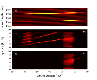
Figure 1: (a) Optical spectrum of the dual-mode two-section device as the device current is varied. The bias applied to the absorber section is 0 V. (b),(c) Corresponding power spectra of the long ($\nu_{2}$) and short ($\nu_{1}$) wavelength primary modes.

We label the short and long wavelength primary modes of the device as $\nu_{1}$ and $\nu_{2}$ respectively. From Fig. 1 (a) we see that the long wavelength mode of the device reaches threshold first at a drive current of $30$ mA. The two primary lasing modes are located near 1550 nm and 1544 nm and they have a spacing of six fundamental cavity modes. These primary modes dominate the spectrum throughout the parameter region of interest. The corresponding power spectral densities for each of the primary modes are shown in Fig. 1 (b) and (c). Structure appears in the power spectral density of $\nu_{2}$ at approximately 35 mA, indicating the onset of dynamical modulation with a frequency of c. $1.5$ GHz. This transition is also reflected in a clear spectral broadening visible in the optical spectrum of the mode. We identify these dynamics as single mode self-pulsations, which appear following a region of constant output in mode $\nu_{2}$ at threshold. The self-pulsations are initially sinusoidal and their frequency increases gradually with device current until a further transition at c. 45 mA. Near this value of the device current a discontinuity appears in the frequency of the intensity modulation, which subsequently increases again until a device current of 70 mA, where a dramatic switch to a region of dual-mode dynamics is observed. In the region of dual-mode dynamics the power spectra become symmetric with a large range of frequencies present, including a signature of low-frequency modulation in the 100 MHz range. This region extends over a current range of approximately 10 mA, with the dynamics switching abruptly to the short wavelength mode $\nu_{1}$ near 80 mA. Following the dual-mode region we observe a single peak in the intensity power spectrum that gradually diminishes in strength. This indicates that, for the largest values of the device current shown, we have reached a state of constant output on the mode at short wavelength.

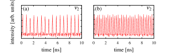
(a)

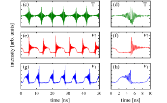
(b)

Figure 2: (a),(b) Measured time traces for the long wavelength mode $\nu_{2}$ for a device current in the gain section of $44$ and $59$ mA respectively. (c),(d) Time traces of the total intensity at a current of $75$ mA in the gain section. (e)-(h) Mode resolved time traces at a current of $75$ mA in the gain section. The bias applied to the absorber section is $0$ V in all cases.

Representative time traces for the intensity of the long wavelength mode in the first and second regions of dynamics are shown in Fig. 2 (a) and (b). The device currents are $44$ and $59$ mA respectively. Fig. 2 (a) shows characteristic self-pulsation dynamics, where the intensity reaches small values between pulses and the pulse duration is significantly less than the interval between pulses. The dynamics in the second region as shown in Fig. 2 (b) are also strongly modulated but they are much closer to sinusoidal than in the region of self-pulsations.

Time traces of the total intensity and of the individual modes taken from the region of dual-mode dynamics are shown in Fig. 2. (c-h). The device current in the long contact for these measurements was $75$ mA. One can see that the total intensity experiences regular bursts of fast pulsations that are modulated by a much lower frequency envelope. The individual modes in this dynamical state display a distinctive symmetric saw-tooth structure, where each mode closely follows a time-reversed trajectory of the other. One can see that there is a significant antiphase component to these dynamics, as the intensity of the individual modes reaches values close to zero over a considerable interval, whereas the total intensity is modulated around a finite background level.

III Modelling of the device response

Modelling the dynamics of our experimental system while treating each mode individually is complicated by the relatively large number of independent parameters javaloyes_10 ; stolarz_11 . However, we have successfully modelled the dynamics of dual-mode devices with optical injection and feedback in past work osborne_09 ; brandonisio_12 , and the LSA model provides a guide for extending these models to the case of a two-section laser. This model treats the absorber section as an unpumped region with an unsaturated absorption and carrier recovery time that depend on the applied voltage.

We do not believe that undertaking a complete theoretical study of the bifurcation structure of the dual-mode LSA model along the lines of dubbeldam_99 would be practical here. Instead, our goal is to understand the physical roles of the various parameters of the system, and to obtain numerical estimates for these parameters based on a comparison of simulation results with the results of our experiment. In physical units the multimode extension of the LSA model reads

$$\begin{gathered}\dot{S}_{m}=[(1-\rho)\tilde{G}_{m}(N_{g})+\rho\tilde{A}_{m}(N_{q})-\gamma_{m}]S_{m}\\ \dot{N}_{g}=j-\dfrac{N_{g}}{\tau_{s}}-\sum_{m}\tilde{G}_{m}(N_{g})S_{m}\\ \dot{N}_{q}=\quad-\dfrac{N_{q}}{\tau_{q}}-\sum_{m}\tilde{A}_{m}({N}_{q})S_{m}\end{gathered}$$ (1)

Here $S_{m}$ is the photon density, and $N_{g}$ and $N_{q}$ are the carrier densities in the gain and absorber sections respectively. The ratio of the absorber section length to the total device length is given by $\rho$. The total field losses of each mode are $\gamma_{m}=\alpha_{\mbox{\tiny mir}}+\alpha_{\mbox{\tiny int}}+\alpha_{\mbox{\tiny f}}^{m}$, where $\alpha_{\mbox{\tiny mir}}$ are the mirror losses and $\alpha_{\mbox{\tiny int}}$ are the internal losses assumed constant for all modes. Additional losses, $\alpha_{\mbox{\tiny f}}^{m}$, due to the action of the spectral filter are also included. The current density in the gain section is $j$, while the carrier lifetimes in the gain and absorber sections are $\tau_{s}$ and $\tau_{q}$ respectively.

Typical profiles of the gain and absorption spectra in a semiconductor laser of the kind we consider are shown schematically in Fig. 3. The negative offset of the gain function at long wavelength gives an estimate of the background losses, $\alpha_{\mbox{\tiny int}}$. Here we have indicated the locations of the two primary modes of the laser. To define the dispersion of gain and absorption, we first fix a reference carrier density value, $N_{g}^{\mbox{\tiny thr}}$, in order to define the dispersion of the gain profile for our model. We take this reference value to be the threshold carrier density for the device assuming a transparent absorber section, and define the mode with the largest material gain at this carrier density as our reference mode, $m_{0}$. The threshold carrier density defines a reference value for the modal gain: $\tilde{G}_{\mbox{\tiny$m_{0}$}}(N_{g}^{\mbox{\tiny thr}})=(1-\rho)^{-1}\gamma_{\mbox{\tiny$m_{0}$}}$, and a set of modal differential gain values, $\tilde{g}_{gm}$. The gain function for each mode can then be linearized around the reference value of the carrier density so that $\tilde{G}_{m}(N_{g})=\tilde{G}_{m}(N_{g}^{\mbox{\tiny thr}})+\tilde{g}_{gm}(N_{g}-N_{g}^{\mbox{\tiny thr}})$. Dispersion in the modal absorption is included by defining $\tilde{A}_{m}(N_{q})=\tilde{g}_{qm}N_{q}-A_{m}^{0}$, where the differential absorption is $\tilde{g}_{qm}$, and unsaturated losses for each mode, $A_{m}^{0}$, will be determined by the applied voltage.

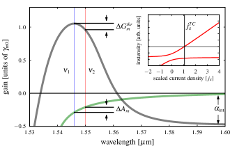
Figure 3: Schematic diagram of the material gain and absorption in a typical semiconductor laser. The locations of the two primary modes of the device $\nu_{1}$ and $\nu_{2}$ are indicated. The model parameters that describe the dispersion of the modal gain and absorption are also highlighted. Inset: Branches of equilibrium solutions of the single mode LSA model for typical parameters considered here. The vertical line is the lasing threshold, $j_{s}^{\mbox{\tiny TC}}$, where the zero field solution becomes unstable.

To derive normalized equations, we rescale time in units of the photon decay rate of a plain FP cavity without spectral filtering: $\gamma=\alpha_{\mbox{\tiny mir}}+\alpha_{\mbox{\tiny int}}$. We define the normalized pump current, $p=(j-j_{\mbox{\tiny thr}})/j_{\mbox{\tiny thr}}\equiv j_{s}-1$, where $j_{\mbox{\tiny thr}}=N_{g}^{\mbox{\tiny thr}}/\tau_{s}$, and we define the normalized carrier densities in each section of the device: $n_{g}=(N_{g}-N_{g}^{\mbox{\tiny thr}})/N_{g}^{\mbox{\tiny thr}}$ and $n_{q}=(N_{0}-N_{q})/N_{g}^{\mbox{\tiny thr}}$, where $N_{0}=A_{m_{0}}^{0}/\tilde{g}_{qm_{0}}$. In normalized units the equations then read

$$\begin{gathered}\dot{I}_{m}=[(1-\rho)G_{m}(n_{g})+\rho A_{m}({n}_{q})-\gamma_{m}^{{}^{\prime}}]I_{m}\\ T\dot{n}_{g}=p-n_{g}-\sum_{m}G_{m}(n_{g})I_{m}\\ T\dot{n}_{q}=\Delta(q_{0}-n_{q})+\sum_{m}A_{m}({n}_{q})I_{m}\end{gathered}$$ (2)

where $q_{0}=\frac{N_{0}}{N_{g}^{\mbox{\tiny thr}}}$, $T=\gamma\tau_{s}$, and $\Delta=\tau_{s}/\tau_{q}$. In these equations the normalized gain functions are

$$G_{m}(n_{g})=G_{m}(n_{g}^{\mbox{\tiny thr}})+g_{gm}N_{g}^{\mbox{\tiny thr}}n_{g}$$

where $G_{m}(n_{g}^{\mbox{\tiny thr}})=\gamma^{-1}\tilde{G}_{m_{0}}^{\mbox{\tiny thr}}+\Delta G_{m}^{\mbox{\tiny thr}}$, $\gamma_{m}^{{}^{\prime}}=\gamma_{m}/\gamma$, and $g_{gm}=\tilde{g}_{gm}/\gamma$. Here $\Delta G_{m}^{\mbox{\tiny thr}}\equiv\gamma^{-1}(\tilde{G}_{m}^{\mbox{\tiny thr}}-\tilde{G}_{m_{0}}^{\mbox{\tiny thr}})$ describes the dispersion of the reference linear gain profile. The normalized modal absorption functions are

$$A({n}_{q})=-g_{qm}N_{g}^{\mbox{\tiny thr}}n_{q}+(g_{qm}-g_{qm_{0}})N_{0}-\gamma^{-1}\Delta A_{m}^{0}$$

where $g_{qm}=\tilde{g}_{qm}/\gamma$, and $\Delta A_{m}^{0}=A_{m}^{0}-A_{m_{0}}^{0}$. Here the normalized carrier density in the absorber section is defined so that the modal absorption is linearized around the saturated value for the reference mode. Note that the phase space of system (2) contains two invariant three dimensional sub-manifolds, defined by $I_{m}=0$, for $m=\{1,2\}$. The dynamics on each of these sub-manifolds reduces to the single-mode LSA system, and for this reason we will refer to these sub-manifolds as the single-mode manifolds of the system.

Based on previous estimates obtained for similar devices osborne_09 , we take the carrier lifetime in the gain section, $\tau_{s}$ = 1 ns. The mirror losses of the device are calculated to be $\alpha_{m}=13.8\mbox{ cm}^{-1}$, and we estimate the internal losses to be $\alpha_{\mbox{\tiny int}}=9.2\mbox{ cm}^{-1}$. These losses determine the cavity decay rate for the plain FP laser to be $\gamma=2\times 10^{11}s^{-1}$, and $T\simeq 200$. In order to define the losses due to spectral filtering and to fix the value of $N_{g}^{\mbox{\tiny thr}}$, we compared our results with threshold data from a plain two-section FP laser. With a uniform current density over the full device length, the threshold current of the FP laser was 13.5 mA. With a bias of 0 V applied to the absorber section, the threshold increased to 17 mA, with the peak emission at 1557.5 nm. The scale of $N_{g}$ is defined so that the differential gain at threshold for the single section FP is equal to 1 in normalised units. We therefore set $N_{g}^{\mbox{\tiny thr}}$ equal to 2.2 based on estimates of the increase in the carrier density necessary to reach the defined threshold level at the wavelength of the reference mode. This estimate was made by taking the losses due to spectral filtering $\alpha_{f}^{\mbox{\tiny m}}=10\mbox{ cm}^{-1}$, and using an approximate model for the semiconductor susceptibility balle_98 . This model allowed us to account for the large blue-shift of the gain peak from its position in the FP laser at threshold. We note that the measured increase in threshold of the dual-mode device, the placement of the spectral filter and the large separation between the selected modes are all factors that suggest large unsaturated absorption and enhanced dispersion of the model parameters.

The carrier lifetime in the absorber section can be much shorter than in the gain section, with a strong dependence on the applied bias karin_94 . We fix the carrier lifetime in the absorber section to be 50 ps, so that $\Delta=20$. However, provided $\Delta$ is not close to one, we have found our results are not dependent on the precise value of this quantity. In order to complete the model we must specify the values of the linear gain, unsaturated absorption, and the differential gain and absorption for each primary mode of the device. Because of the large size of this parameter space, we begin by considering the dynamics of two coupled modes with similar parameters. Guided by the known dispersive properties of the semiconductor susceptibility, and by the observed behavior of the device, we then make a series of further adjustments to these parameters until we have obtained satisfactory agreement with measured data.

IV Bifurcations of a dual-mode semiconductor laser with a saturable absorber

For our numerical simulations, the parameters describing the gain function at the position of the reference mode, $\nu_{1}$, are fixed. To begin we assume a flat gain and absorption curve and we examine the effects of dispersion in the differential gain and absorption on the dynamics of the coupled system. From Fig. 1 we see that in our experiment the device begins to lase with constant intensity output on the long wavelength mode, before entering a region of SP. At the largest values of the pump current the intensity switches to short wavelength. With equal linear gain and unsaturated absorption, the mode with the largest differential gain will reach threshold first. On the other hand, a larger differential absorption will mean that a mode will saturate its losses more quickly above threshold and thereby dominate at larger pump values. To reproduce this behaviour, we set the differential gain and absorption of mode $\nu_{1}$ in normalised units to be $1.0$ and $1.2\rho^{-1}$ respectively. The ratio of these quantities for mode $\nu_{1}$ is then $s_{1}\equiv g_{q1}/g_{g1}$ = 22. We set the differential gain and absorption of $\nu_{2}$ to be $1.4$ and $0.6\rho^{-1}$ respectively so that $s_{2}$ = 7.8. The remaining parameters values we choose to begin are $A_{\mbox{\tiny[1,2]}}^{0}=0.2\gamma$ and $\Delta G_{m\mbox{\tiny[1,2]}}^{\mbox{\tiny thr}}=0$. Note that the differential gain in normalised units is likely to be less than unity given the higher current density at threshold in the dual-mode device. We have decided not to make this correction in order to make the comparison of the various model parameters more transparent. We have confirmed that our results are largely independent of the precise values chosen for $g_{g1}$, provided the other differential quantities are scaled accordingly.

While the LSA model can predict the appearance of self-pulsations immediately at threshold ueno_85 ; dubbeldam_99 , our chosen parameter values are consistent with the observation of a narrow region of constant output at threshold in our experiment. If we consider a single mode system, the zero field equilibrium solution of these equations is stable until a transcritical bifurcation at a threshold value of the pump

$$p_{\mbox{\tiny TC}}=\frac{\rho A_{m}^{0}}{(1-\rho)g_{g}\gamma N_{g}^{\mbox{\tiny thr}}}.$$

The inset of Fig. 3 shows the branches of single mode equilibrium solutions of Eqn (2) taking the model parameters for mode $\nu_{1}$. Here $\Delta$ exceeds a minimum value given by

$$\Delta=s\frac{q_{0}^{{}^{\prime}}}{1+q_{0}^{{}^{\prime}}}.$$

where $q_{o}^{{}^{\prime}}=\gamma^{-1}\rho A_{m}^{\scriptscriptstyle 0}$. This condition leads to constant output at threshold, as the upper branch of equilibrium solutions takes physical values after exchanging stability with the zero field solution. A further bifurcation to SPs will then occur provided there is sufficient saturable absorption in the system. We will find that the stability of the single-mode equilibria plays a fundamental role in organising the dynamics in our device, and we will therefore present numerical bifurcation diagrams for each of the single-mode solutions of our model as we vary the model parameters for each mode.

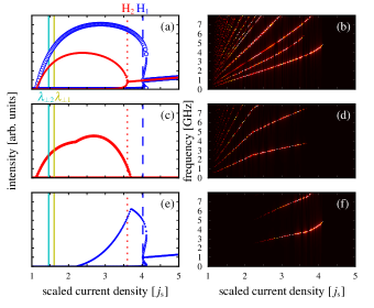
Figure 4: Left panels: Simulated bifurcation diagrams. Right panels: Power spectral densities. (a),(b): Single-mode dynamics. (c),(d): Long wavelength mode $\nu_{2}$. (e),(f): Short wavelength mode $\nu_{1}$.

Numerical bifurcation diagrams and intensity power spectra obtained with our first set of parameters are shown in Fig. 4. Figs 4 (a) and (b) describe the dynamics of both of the primary modes restricted to their respective single mode manifolds, obtained by setting the intensity of the inactive mode to zero for the time evolution of Eqn (2). In Fig. 4 (a), as expected, the single mode dynamics of both modes exhibit threshold behaviour similar to the observed behaviour of the long wavelength mode in our experiment, with a region of constant output found after the zero field solution becomes unstable. Following this region, they enter a region of SPs at the location of the first Hopf bifurcation, and the SP region is bounded in each case by a second Hopf bifurcation at larger pump current. In Fig. 4, dashed and dotted lines labelled H₁ and H₂ indicate the second Hopf bifurcation points that bound the SP region at larger pump values for each mode.

Mode resolved numerical bifurcation diagrams and power spectra for the two modes in the full coupled mode system are shown in Fig. 4 (c)-(f). Chosen parameters ensure that the long wavelength mode reaches threshold first, and because the second mode is initially suppressed, mode $\nu_{2}$ reproduces the dynamics found in the single mode system. However, before the region of single mode SP ends at the second Hopf bifurcation shown in Fig. 4 (a), the dynamics become dual-mode, with the SP intensity gradually switching across to the shorter wavelength mode $\nu_{1}$ as the pump is increased further. This dual-mode region comes to an end shortly after a pump value of $j_{s}=3$ where the system enters a region of single mode SP on $\nu_{1}$. The region of SP dynamics finally ends at the subcritical Hopf bifurcation of $\nu_{1}$, and the dynamics switch to constant output in mode $\nu_{1}$ for large values of the pump current.

In the power spectrum of Fig. 4 (d) we see that at the onset of SPs, they occur with a frequency of c. $500$ MHz, with a linear increase in each interval of single or dual-mode dynamics thereafter, and reaching a value of c. 5 GHz at $j_{s}=4.25$. We can compare this evolution with the dependence of the relaxation oscillation frequency, which, neglecting the effects of saturable absorption, is given by

$$\omega_{\mbox{\tiny RO}}=\sqrt{\frac{(1-\rho)g_{g}N_{g}^{\mbox{\tiny thr}}p}{T}}.$$ (3)

At $j_{s}=4.25$, the result is approximately 6 GHz, which is a reasonable estimate of the SP frequency in this model. Note however that the close to linear increase of the numerical SP frequency contrasts with the square-root dependence of the above expression.

If we compare the numerical variation of the SP frequency with our experiment, we see that the measured SP frequency appears with a large value of c. 1.5 GHz, and that it then remains relatively constant. Our simulations therefore underestimate the SP frequency at onset, and overestimate its rate of increase. One can also see that the extent of the SP region that we find numerically is much larger than the measured value. While the measured variation of the SP frequency may be partly due to an uncharacteristic behavior of our device, it should be noted that we cannot expect to obtain quantitative agreement with experiment using the LSA model. We have confirmed this by comparing the results of numerical simulations made using the LSA model and the delay-differential model of vladimirov_04 . For example, using experimentally calibrated parameters appropriate to a self-pulsating FP laser, we have found that the LSA model will in general predict a far larger SP region, with a larger SP frequency than the delay-differential model. In addition, while we can adjust unknown parameters such as the absorber recovery time to match numerical and experimental results in the case of the delay differential model, this is in general not possible when using the LSA model. This comparison emphasizes the added importance of accounting for the large changes in gain and loss that can occur in two-section semiconductor lasers, where SP dynamics involve strong saturation of the absorption for typical parameters.

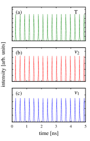
(a)

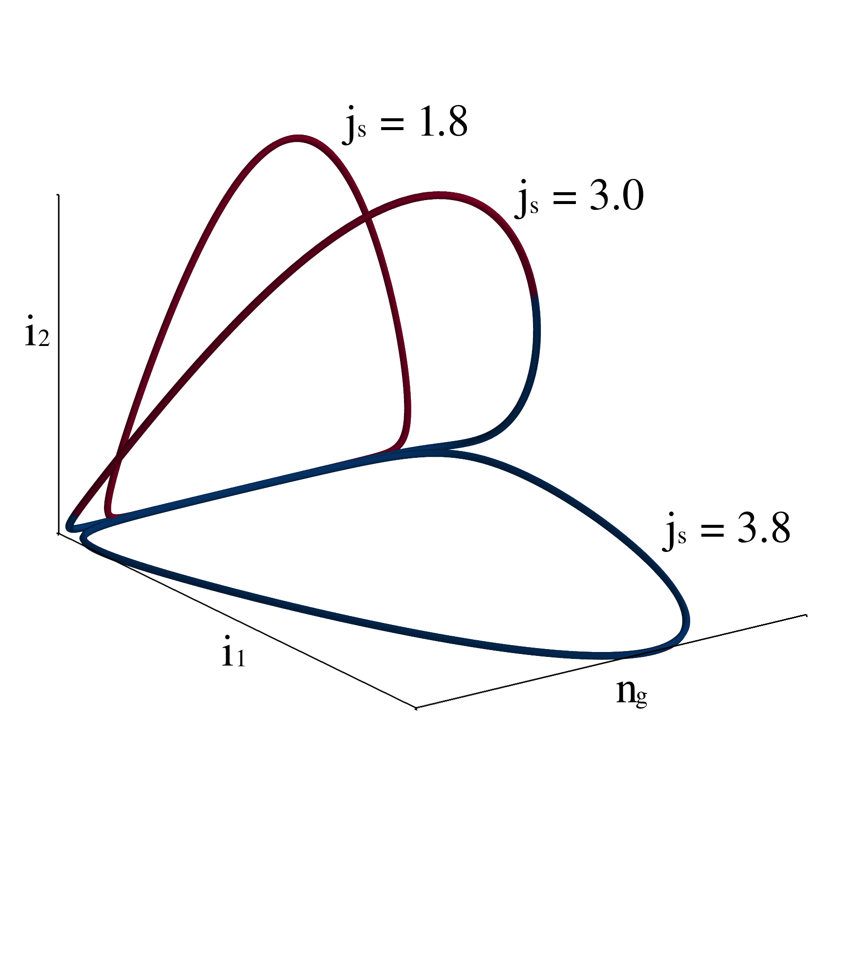
(b)

Figure 5: Left: Simulated time traces of the total intensity (upper panel), and of the individual modes (center and lower panels). The pump current value is $j_{s}$ = 3. Right: Phase space diagrams for three values of the pump current as shown.

Time traces taken from the center of the dual-mode region with $j_{s}=3$ are shown in the left panel of Fig. 5, while the right hand panel of Fig. 5 shows a phase space representation of the dynamics for three pump values, taken before, during and after the transition from $\nu_{2}$ to $\nu_{1}$. We see that the intensity shifts continuously from one mode to the other through a region of in-phase SP. As expected, the gradual transition of the dynamics from $\nu_{2}$ to $\nu_{1}$ that we observe in these simulations leads to agreement with the experimental measurements of Fig. 1 near threshold and at large values of the pump.

Valuable insight into what factors can lead to better agreement with experiment can be gained from a close examination of the time traces presented in Fig. 2 (c-h). From these figures, we see that for the majority of the orbit duration the intensity is close to the single mode manifold of one mode or the other. In Fig. 2 (f) we see the large intensity oscillations of $\nu_{2}$ decaying toward a state with almost constant output, and the intensity then quickly switching to a similar state in $\nu_{1}$ from which the oscillations grow again. The clear observation of this near single mode state with constant output at the beginning and end of these bursts of pulsations suggests that the single mode equilibrium states of (2) may be playing an important role in organising the observed dynamics. In particular, given the presence of symmetric invariant sub-manifolds in the phase-space, we should examine the dependence of the transverse stability of the single mode equilibrium solutions on the model parameters.

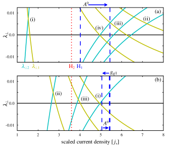
Figure 6: Effect of including dispersion in model parameters on the transverse Lyapunov exponent and the location of the second Hopf bifurcation of each single-mode equilibrium of the model. Dashed and dotted lines indicate Hopf bifurcations of $\nu_{1}$ and $\nu_{2}$ respectively. Solid lines are the transverse Lyapunov exponents of each mode as indicated. (a) (i) Parameters as in Fig. 4, $\text{(ii)-(iv)}A_{\mbox{\tiny 1}}^{0}=0.35\gamma$ and $\Delta G_{m2}^{\mbox{\tiny thr}}=[\text{(ii)}0,\text{(iii)}-0.25,\text{(iv)}-0.5]\gamma^{-1}$. (b) (i) Parameters as in (iv) of (a), $\text{(ii), (iii) }g_{q1}=1.5$, and $A_{\mbox{\tiny 1}}^{0}=\text{(ii)}0.35\gamma,\>\text{(iii)}0.4\gamma$.

The transverse stability of the single-mode equilibrium solution for mode $\nu_{i}$, $I_{i}^{0}$, is determined by the sign of its transverse Lyapunov exponent

$$\lambda_{\perp i}=(1-\rho)G_{j}(I_{i}^{0})+\rho A_{j}(I_{i}^{0})-\gamma_{j}$$ (4)

where $\{i,j\}=\{1,2\}$ and mode $\nu_{i}$ is transversally stable for negative values of $\lambda_{\perp i}$. For illustration purposes, we have plotted and labelled solid lines in Fig. 4 that indicate where the changes in transverse stability occur for the chosen parameter values. Note that in this case $\nu_{2}$ becomes transversally unstable while $\nu_{1}$ becomes transversally stable with increasing $j_{s}$. The impact of dispersion of linear gain and unsaturated absorption on the dynamics of our model can be illustrated by a plot of the locations of the Hopf bifurcations and changes in transverse stability of the single mode equilibrium solutions as the relevant parameters are varied. In Fig. 3, the physical dispersion of the unsaturated absorption suggests a larger value of $A^{0}$ for $\nu_{1}$, and stability changes for both modes obtained with $A_{\mbox{\tiny 1}}^{0}$ increased to a value of $0.35\gamma$, and $\Delta G_{m2}^{\mbox{\tiny thr}}$ ranging from $0$ to $-0.5\gamma^{-1}$ are shown in Fig. 6 (a). In these figures vertical dashed and dotted lines indicate the locations of the second Hopf bifurcation for $\nu_{1}$ and $\nu_{2}$ respectively. Curved solid lines plot the value of the transverse Lyapunov exponent for each mode as indicated, with sign changes of these quantities indicating changes in transverse stability. One can see the impact that a change of only $0.5\mbox{ cm}^{-1}$ to the linear gain profile has on the transverse stability properties of these modes. The cumulative net effect of these changes is that there is now a much larger separation between the second Hopf bifurcation points of both modes. In addition, the sign changes of the transverse Lyapunov exponents for each mode now occur between the pair of Hopf bifurcations.

Numerical bifurcation diagrams obtained for parameter set (iv) of Fig. 6 (a) are plotted in in the left hand panels of Fig. 7. Here, $A_{\mbox{\tiny 1}^{0}}=0.35\gamma$, $\Delta G_{m\mbox{\tiny 2}}^{\mbox{\tiny thr}}=-0.5\gamma^{-1}$, and all other parameters are unchanged from Fig. 4. The increased unsaturated losses mean that mode $\nu_{1}$ is suppressed for longer and, in contrast to the results of Fig. 4, mode $\nu_{2}$ now completes a region of single-mode SP bounded by two single mode Hopf bifurcations. Following the SP region, the system enters a region of single-mode constant output. However, as we increase the pump current still further we find the dynamics are dramatically “blown-out” from the single mode manifold and we enter a region of coupled dynamics in both modes. The location of the blow-out is determined by the loss of transverse stability of $\nu_{2}$, and this point is located shortly after $\nu_{1}$ has become transversally stable. The region of dual-mode dynamics is bounded at larger values of the pump current by a subcritical Hopf bifurcation of mode $\nu_{1}$.

In order to compare the measurements of Fig. 2 in the dual-mode region with the simulation results of Fig. 7, we have plotted mode-resolved and total intensity time traces with $j_{s}$ = 5.1 in the right-hand panels of Fig. 7. The similar nature of the two dynamical states is clear, with the numerical results reproducing the observed bursts of fast pulsations in the total intensity and also the switching sequence with the intensity rising on the short wavelength mode before switching and falling on the long wavelength mode. However, the frequency of the bursts that we find numerically is much too low at around 10 MHz. In addition, the numerical bifurcation sequence in not in full agreement with our measurements. We find a large region of constant output between the second Hopf bifurcation of $\nu_{2}$ and the onset of coupled mode dynamics and we also do not see any evidence of a discontinuity in the frequency of the intensity modulation at intermediate values of the pump.

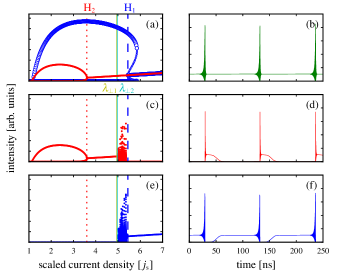
Figure 7: Left panels: Simulated bifurcation diagrams. Right panels: Intensity time traces. (a) Single-mode dynamics. (b) Total intensity. (c),(d) Long wavelength mode $\nu_{2}$. (e),(f) Short wavelength mode $\nu_{1}$.

By further adjustment of parameters we can shift the point where the transverse stability of the equilibrium state of $\nu_{1}$ changes at smaller values of the pump. This will result in a narrowing of the region of constant output in agreement with experiment. Fig. 6 (b) illustrates the effect of an increase in $g_{q1}$ combined with a further increase of $A_{\mbox{\tiny 1}}^{0}$. The net effect of these adjustments is that the positions of the Hopf bifurcations remain largely the same, but the changes of transverse stability happen much closer in pump current to the second Hopf bifurcation of $\nu_{2}$. Numerical bifurcation diagrams and intensity power spectra with $g_{q1}=1.5$ and $A_{\mbox{\tiny 1}}^{0}=0.4$ are shown in Fig. 8. The bifurcation sequence we observe until the change in transverse stability of the single mode equilibrium of $\nu_{2}$ is the same as in Fig. 7. However, instead of a dramatic transition to a region of complex coupled dynamics, in this case we find a very narrow region where a dual-mode equilibrium state of the system is stable. This state appears here for the first time in our simulations, and it appears because the order of the changes in transverse stability of the single-mode equilbiria has been reversed compared to the previous example. We find that the dual-mode equilibrium state quickly evolves into a dual-mode limit cycle at a Hopf bifurcation point. This dual-mode limit cycle is unusual in that the amplitude of $\nu_{1}$ over the cycle is very weak to begin. With a further increase in the pump current, the dual mode limit cycle loses stability, and we observe a dramatic transition to a region of complex coupled dynamics in both modes. As in the previous example, the region of complex dynamics is bounded at a large pump current by a subcritical Hopf bifurcation in $\nu_{1}$.

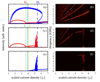
Figure 8: Left panels: simulated bifurcation diagrams. Right panels: Power spectral densities. (a),(b): Single-mode dynamics. (c),(d): Long wavelength mode $\nu_{2}$. (e),(f): Short wavelength mode $\nu_{1}$.

A plot of the mode-resolved and total intensity time traces taken from the region of complex coupled dynamics in Fig. 8 with $j_{s}$ = 5.2 is shown in the left-hand panels of Fig. 9. When compared to our experimental results, there is a greater degree of asymmetry between the dynamics of the two modes in this example. Unlike the previous example however, the frequency of the bursts of fast pulsations of the total intensity is now accurately matched to our experimental results. We note also that the observed bifurcation sequence provides an explanation for the dynamics we found at intermediate values of the pump current in our experiment. We can now see that the discontinuity in the frequency of the intensity modulation of $\nu_{2}$ was due to the momentary appearance of a stable dual-mode steady state in the system, leading to the absence of any structure in the intensity power spectrum over this interval. In addition, we must reinterpret the region after the discontinuity as a dual-mode state with strong intensity modulation, but where the amplitude of the component in $\nu_{1}$ is very weak.

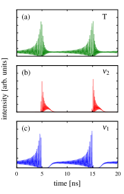
(a)

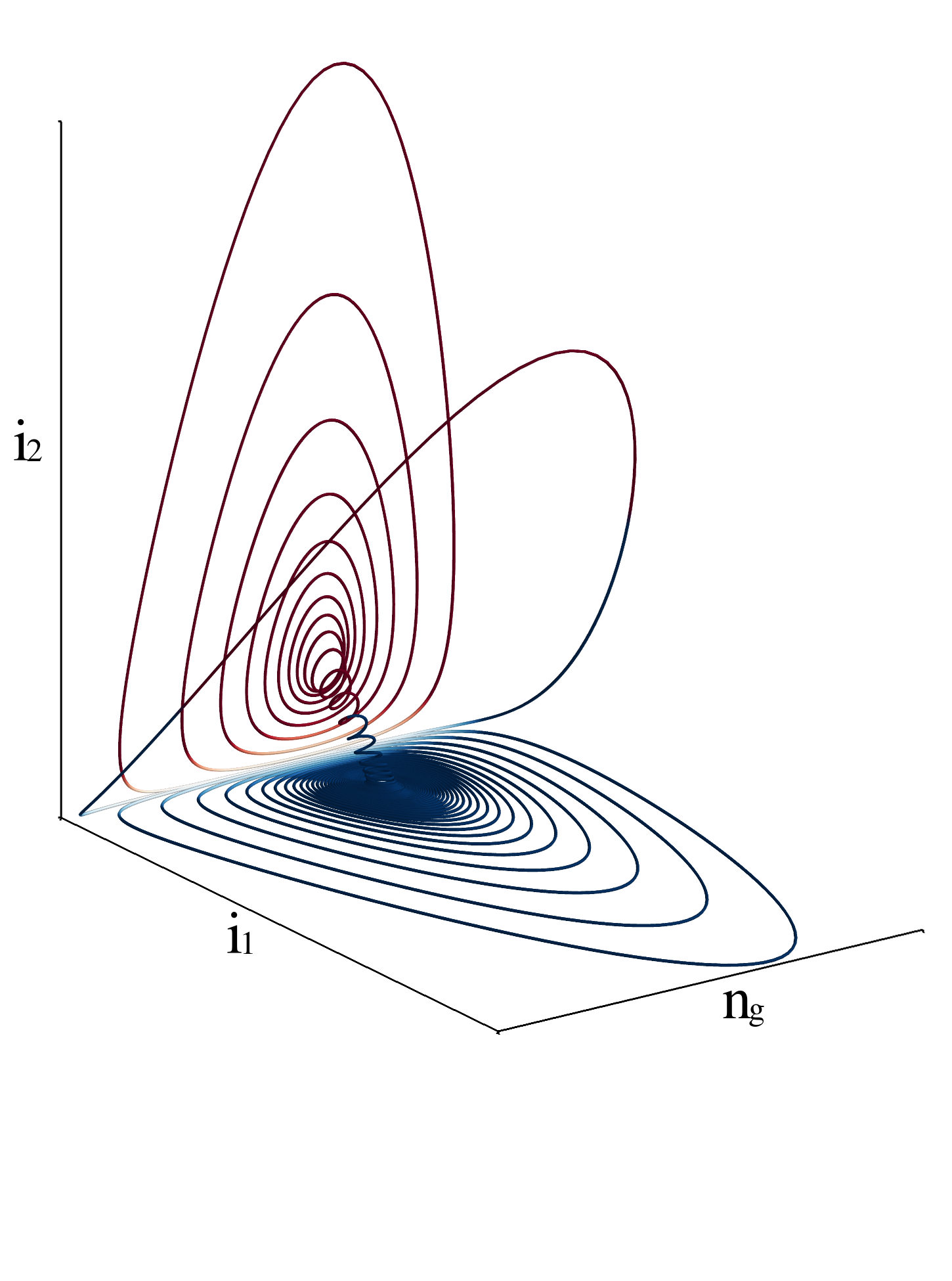
(b)

Figure 9: Left: Simulated intensity time traces. (a) Total intensity. (b) Long wavelength mode $\nu_{2}$. (c) Short wavelength mode $\nu_{1}$. Right: Phase space diagram

The time-traces of Fig. 9 are depicted in a phase-space representation on the right of Fig. 9. If we consider trajectories close to the single-mode equilibrium state of $\nu_{1}$, these trajectories are attracted towards the single mode manifold as the single-mode equilibrium state has a negative transverse Lyapunov exponent. Because this state is unstable in the single-mode manifold, as the trajectory approaches the manifold it is repelled into a spiralling orbit towards the SP limit cycle, which is stable within the $\nu_{1}$ manifold. This is the origin of the fast pulsations that grow from the quasi-single mode steady state of $\nu_{1}$. Once the trajectory approaches the SP limit cycle, it feels the transverse instability of this limit cycle and is ultimately ejected from the region near the single-mode manifold, undergoing a large amplitude excursion where both fields have large intensity. This large excursion leads the trajectory to enter the slow region near zero intensity, where it is drawn towards the single mode manifold of $\nu_{2}$, where the single mode equilibrium state is stable within the manifold. This leads to the cycle of fast pulsations that decay towards the single mode equilibrium state of $\nu_{2}$. Finally, as the trajectory approaches the equilibrium, it is repelled on account of the positive transverse Lyapunov exponent of this state. This repulsion drives the trajectory towards the transversally attracting equilibrium state of $\nu_{1}$ and the cycle begins again. The switch in intensity from $\nu_{2}$ to $\nu_{1}$ is along a corkscrew type trajectory that is wound around the line connecting the equilibrium states in the two single mode manifolds. This winding may be a signature of the dual-mode limit cycle present before the region of complex dynamics.

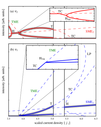
Figure 10: Bifurcation diagrams of $\nu_{2}$ (upper panel) and $\nu_{1}$ (lower panel). Single and dual-mode equilibrium states are labeled $\mbox{SME}_{j}$ and TME respectively. Bifurcation points are single-mode Hopf bifurcations (H), transcritical (TC), dual-mode Hopf bifurcations ($\mbox{H}_{\mbox{\tiny{TM}}}$), Torus bifurcations (T) and limit point (LP). Solid and dashed lines indicate stable and unstable objects respectively. The results of numerical simulations of the coupled system are included as a guide. Solid vertical lines bound the region of complex dual-mode dynamics.

To investigate this question and to shed more light on the bifurcation structure in this system, in Fig. 10 we have plotted numerical continuation results obtained using AUTO auto . These results indicate that the instability of the dual-mode limit cycle leading to complex dynamics is due to a supercritical Torus bifurcation (T). We can also see that the dual-mode limit cycle is present as an unstable object throughout the region of complex dynamics, and that there is evidence for further bifurcations of interest involving this object beyond the boundary of the region of complex dual-mode dynamics. In particular, we can see that the unstable dual-mode limit cycle collides with the unstable branch of single-mode SPs of mode $\nu_{1}$ in a transcritical bifurcation (TC). This results in the unstable branch of single-mode SPs becoming transversally stable for decreasing pump values until the subcritical Hopf bifurcation of $\nu_{1}$ is reached. This narrow region of transverse stability for this unstable branch of SPs may explain the sharp feature near the relaxation oscillation frequency found in the power spectral data of Fig. 1. The diminishing strength of this feature with increasing current could be a result of the growth of the limit cycle away from the location of the stable equilibrium.

Finally, we note that although a complete discussion of the bifurcation structure that organises the dynamics of Fig. 9 is beyond the scope of the current paper, we can highlight a number of interesting parallels with previous work on optically injected dual-mode devices osborne_09 ; blackbeard_12 . Mathematically, this system is also four dimensional, but it features a single, three dimensional invariant manifold corresponding to the single-mode injected system. Despite the lower symmetry of the dual-mode injected system, in the example of osborne_09 , we also found a saw-tooth structure characterized by symmetric but oppositely directed trajectories of the two modes. These dynamics originated in a torus bifurcation of a dual-mode periodic orbit. On the other hand, blackbeard_12 considered an example of bursting dynamics from the region of the single-mode manifold. These dynamics appeared near a cusp-pitchfork bifurcation of limit cycles and a curve of global saddle-node heteroclinic bifurcations. We will present a similar two-parameter bifurcation study of the current system and explore these connections further in future work.

V Conclusions

We have presented an experimental and theoretical study of the dynamics of a dual-mode semiconductor laser with a saturable absorber. The device was a specially engineered Fabry-Perot laser designed to support two primary modes with a large frequency spacing. Fixing the voltage applied to the absorber section, we performed a sweep in drive current in the gain section of the device. We found that the dynamics evolved from familar self-pulsations in a single mode of the device into a complex dynamical state of both modes. By extending the well-known rate equation model for the semiconductor laser with a saturable absorber to the multimode case, we were able to reproduce the observed dynamics, and to show the fundamental role played by material dispersion in both sections of the device in governing their appearance.

Acknowledgments. The authors acknowledge the financial support of Science Foundation Ireland under Grant “SFI13/IF/I2785”.

References

- (1) P. Vasil’ev, “Ultrafast diode lasers,” Artech House, Boston (1996).
- (2) H. Haus, IEEE J. Selected Topics Quantum Electron., 6 1173 (2000).
- (3) E. A. Avrutin, J. H. Marsh, and E. L. Portnoi, IEEE Proc. Optoelectron. 147, 251 (2000).
- (4) T. Miyajima, H. Watanabe, M. Ikeda, and H. Yokoyama, Appl. Phys. Lett. 94, 161103 (2009).
- (5) D. Rachinskii, A. Vladimirov, U. Bandelow, B. Huttl, and R. Kaiser, J. Opt. Soc. Am. B 23, 663 (2006).
- (6) T. Kolokolnikov, M. Nizette, T. Erneux, N. Joly, S. Bielawski, Physica D 219, 13 (2006).
- (7) M. Ueno and R. Lang, J. Appl. Phys. 58, 1689 (1985).
- (8) J. L. A. Dubbeldam and B. Krauskopf, Opt. Comm. 159, 325 (1999).
- (9) V. Z. Tronciu, M. Yamada, T. Ohno, S. Ito, T. Kawakami, and M. Taneya, IEEE J. Quantum Electron. 39, 1590 (2003).
- (10) J. Dorsaz, D. L. Boiko, L. Sulmoni, J.-F. Carlin, W. G. Scheibenzuber, U. T. Schwarz, and N. Grandjean, Appl. Phys. Lett. 98, 191115 (2011).
- (11) J. Mulet and J. Mork, IEEE J. Quantum Electron. 42, 249 (2006).
- (12) J. Javaloyes and S. Balle, IEEE J. Quantum Electron. 46, 1023 (2010).
- (13) A. G. Vladimirov, D. Turaev, and G. Kozyreff, Opt. Lett. 29, 1221 (2004).
- (14) P. M. Stolarz, J. Javaloyes, G. Mezosi, L. Hou, C. N. Ironside, M. Sorel, A. C. Bryce, S. Balle, IEEE Photonics Journ. 3, 1067 (2011).
- (15) A. G. Vladimirov, and D. Turaev Phys. Rev. A 72, 033808 (2005).
- (16) C. Otto, K. Ludge, A. G. Vladimirov, M. Wolfrum, and E. Scholl, New Journ. Phys. 14, 113033 (2012).
- (17) S. O’Brien, S. Osborne, D. Bitauld, N. Brandonisio, A. Amann, R. Phelan, B. Kelly, and J. O’Gorman, IEEE Trans. Microwave Theory Tech. 58, 3083 (2010).
- (18) D. Bitauld, S. Osborne and S. O’Brien, Opt. Lett. 35, 2206 (2010).
- (19) D. Bitauld, S. Osborne and S. O’Brien, Opt. Express 19, 13989 (2011).
- (20) K. Y. Lau, IEEE J. Quantum Electron. 26, 250 (1990).
- (21) E. A. Avrutin, J. M. Arnold and J. H. Marsh, IEEE J. Selected Topics Quantum Electron., 9, 844 (2003).
- (22) S. Osborne, A. Amann, K. Buckley, G. Ryan, S. P. Hegarty, G. Huyet, and S. O’Brien, Phys. Rev. A 79, 023834 (2009)
- (23) N. Brandonisio, P. Heinricht, S. Osborne, A. Amann, and S. O’Brien, IEEE Photonics Journ. 4, 95 (2012).
- (24) S. Balle, Phys. Rev. A 57, 1304 (1998).
- (25) J. R. Karin, R. J. Helkey, D. J. Derickson, R. Nagarajan, D. S. Allin, J. E. Bowers, and R. L. Thornton, Appl. Phys. Lett. 64, 677 (1994).
- (26) E. J. Doedel, A. R. Champneys, T. Fairgrieve, Yu. Kuznetsov, B. Oldeman, R. Pfaffenroth, B. Sandstede, X. Wang, and C. Zhang. Technical report, Concordia University, Montreal, Canada (2007) http://indy.cs.concordia.ca/auto/.
- (27) N. Blackbeard, S. Osborne, S. O’Brien, and A. Amann, arXiv:1210.4484 (2012).