A Conforming Finite Element Discretization of the Streamfunction Form of the Unsteady Quasi-Geostrophic Equations

Abstract.

This paper presents a conforming finite element semi-discretization of the streamfunction form of the one-layer unsteady quasi-geostrophic equations, which are a commonly used model for large-scale wind-driven ocean circulation. We derive optimal error estimates and present numerical results.

1. Introduction

The quasi-geostrophic equations (QGE), a standard simplified mathematical model for large scale oceanic and atmospheric flows [6, 17, 18, 20], are often used in climate models [7]. We consider a finite element (FE) discretization of the QGE to allow for better modeling of irregular geometries. Indeed, it is important to represent features like coastlines in ocean models; numerical artifacts can result from stepwise boundaries, which can affect ocean circulation predictions over long time integration [1, 8, 22].

Most analyses of the QGE have been done on the mixed streamfunction-vorticity rather than the pure streamfunction form. This work focuses on the latter, which has the advantage of known optimal error estimates (see the error estimate 13.5 and Table 13.1 in [14]). However, the disadvantage of not using a mixed formulation is that the pure streamfunction form of the QGE is a fourth-order problem: this necessitates the use of a $C^{1}$ FE space for a conforming FE discretization.

In what follows we first introduce, in Section 1, the streamfunction-vorticity form of the QGE and its nondimensionalization, followed by the pure streamfunction form of the QGE. In Section 3 we introduce the functional setting and the FE discretization in space. From there, we develop optimal error estimates in Section 4 followed by, in Section 5, numerical verification of the error estimates developed in Section 4.

2. The Quasi-Geostrophic Equations

The QGE are usually written as follows (e.g., equation (14.57) in [20], equation (1.1) in [17], equation (1.1) in [21], and equation (1) in [13]):

$$\frac{\partial q}{\partial t}+J(\psi,q) =A\,\Delta q+F$$ (1)

$$q =\Delta\psi+\beta\,y,$$ (2)

where $q$ is the potential vorticity, $\psi$ is the velocity streamfunction, $\beta$ is the coefficient multiplying the $y$-coordinate (which is oriented northward) in the $\beta$-plane approximation (4), $F$ is the forcing, $A$ is the eddy viscosity parameterization, and $J(\cdot,\cdot)$ is the Jacobian operator given by

$$J(\psi,q):=\frac{\partial\psi}{\partial x}\,\frac{\partial q}{\partial y}-\frac{\partial\psi}{\partial y}\,\frac{\partial q}{\partial x}.$$ (3)

The $\beta$-plane approximation reads

$$f=f_{0}+\beta\,y,$$ (4)

where $f$ is the Coriolis parameter and $f_{0}$ is the reference Coriolis parameter (see the discussion on page 84 in [5] or Section 2.3.2 in [20]). As noted in Chapter 10.7.2 in [20] (see also [19]), the eddy viscosity parameter $A$ in (1) is usually several orders of magnitude higher than the molecular viscosity. This choice allows the use of a coarse mesh in numerical simulations. The horizontal velocity $\mathbf{u}$ can be recovered from $\psi$ and $q$ by the formula

$$\mathbf{u}:=\nabla^{\perp}\psi=\left(\begin{matrix}-\frac{\partial\psi}{\partial y}\\ \frac{\partial\psi}{\partial x}\end{matrix}\right).$$ (5)

The computational domain considered in this report is the standard [13] rectangular, closed basin on a $\beta$-plane with the $y$-coordinate increasing northward and the $x$-coordinate eastward. The center of the basin is at $y=0$, the northern and southern boundaries are at $y=\pm\,L$, respectively, and the western and eastern boundaries are at $x=0$ and $x=L$ (see Figure 1 in [13]).

We are now ready to nondimensionalize the QGE (1)-(2). There are several ways of nondimensionalizing the QGE, based on different scalings and involving different parameters (see standard textbooks on geophysical fluid dynamics, such as [6, 17, 18, 20]). Since the FE error analysis in this report is based on a precise relationship among the nondimensional parameters of the QGE, we present a careful nondimensionalization of the QGE below. We first need to choose a length scale and a velocity scale– the length scale we choose is $L$, the width of the computational domain. To define the velocity scale, we first need to specify the forcing term $F$ in (1). To this end, we follow the presentation in Section 14.1.1 in [20] and assume that $F$ is the wind-stress curl at the top of the ocean:

$$F=\dfrac{1}{\rho}\left(\dfrac{\partial\tau^{y}}{\partial x}-\dfrac{\partial\tau^{x}}{\partial y}\right),$$ (6)

where $\rho$ is the density of the fluid, $\boldsymbol{\tau}=(\tau^{x},\tau^{y})$ is the wind-stress at the top of the ocean (see also Section 2.12 and equation (14.3) in [20] and Section 5.4 in [5]) and is measured in $N/m^{2}$ (e.g., page 1462 in [13]). To determine the characteristic velocity scale, we use the Sverdrup balance given in equation (14.20) in [20] (see also Section 8.3 in [5]):

$$\beta\int vdz=\dfrac{1}{\rho}\left(\dfrac{\partial\tau^{y}}{\partial x}-\dfrac{\partial\tau^{x}}{\partial y}\right),$$ (7)

in which the velocity component $v$ is integrated along the depth of the fluid. The Sverdrup balance in (7) represents the balance between wind-stress (i.e., forcing) and $\beta$-effect, which yields the Sverdrup velocity

$$U:=\dfrac{\tau_{0}}{\rho H\beta L},$$ (8)

where $\tau_{0}$ is the amplitude of the wind stress and $H$ is the depth of the fluid. It is easy to check that the Sverdrup velocity defined in (8) has velocity units. We note that the same Sverdrup velocity is used in equation (8-11) in [5] and on page 1462 in [13] (the latter has an extra $\pi$ factor due to the particular wind forcing employed). The Sverdrup velocity (8) will be used as the characteristic velocity scale in the nondimensionalization. Once the length and velocity scales are chosen, the variables in the QGE (1)-(2) can be nondimensionalized as follows:

$$x^{*}=\frac{x}{L},\quad y^{*}=\frac{y}{L},\quad t^{*}=\frac{t}{L/U},\quad q^{*}=\frac{q}{\beta\,L},\quad\psi^{*}=\frac{\psi}{U\,L},$$ (9)

where a superscript ^∗ denotes a nondimensional variable. We denote derivatives taken with respect to nondimensional coordinates by $\Delta^{*}$ and $J^{*}(\cdot,\cdot)$. Using (9), the nondimensionalization of (2) is

$$\beta\,L\,q^{*}=\frac{1}{L^{2}}\,\Delta^{*}(U\,L\,\psi^{*})+\beta\,(L\,y^{*}).$$ (10)

Dividing (10) by $\beta\,L$, we get:

$$q^{*}=\left(\frac{U}{\beta\,L^{2}}\right)\,\Delta^{*}\psi^{*}+y^{*}.$$ (11)

Defining the Rossby number $Ro$ as

$$Ro:=\frac{U}{\beta\,L^{2}},$$ (12)

equation (11) becomes

$$q^{*}=Ro\,\Delta^{*}\psi^{*}+y^{*}.$$ (13)

Then we nondimensionalize (1). We start with the left-hand side:

$$\dfrac{\partial q}{\partial t} =(\beta U)\dfrac{\partial q^{*}}{\partial t^{*}},$$ (14)

$$J(\psi,q) =\dfrac{\partial\psi}{\partial x}\dfrac{\partial q}{\partial y}-\dfrac{\partial\psi}{\partial y}\dfrac{\partial q}{\partial x}=U\dfrac{\partial\psi^{*}}{\partial x^{*}}\beta\dfrac{\partial q^{*}}{\partial y^{*}}-U\dfrac{\partial\psi^{*}}{\partial y^{*}}\beta\dfrac{\partial q^{*}}{\partial x^{*}}=(\beta U)J^{*}(\psi^{*},q^{*}).$$ (15)

Next, we nondimensionalize the right-hand side of (1). The first term can be nondimensionalized as

$$A\Delta q=A\left(\frac{\partial^{2}q}{\partial x^{2}}+\frac{\partial^{2}q}{\partial y^{2}}\right)=A\left(\frac{1}{L^{2}}\frac{\partial^{2}}{\partial{x^{*}}^{2}}(\beta Lq^{*})+\frac{1}{L^{2}}\frac{\partial^{2}}{\partial{y^{*}}^{2}}(\beta Lq^{*})\right)=A\frac{\beta}{L}\Delta^{*}q^{*}.$$ (16)

Thus, inserting (14)-(16) in (1), we get

$$(\beta\,U)\,\frac{\partial q^{*}}{\partial t^{*}}+(\beta\,U)\,J^{*}(\psi^{*},q^{*}) =A\,\frac{\beta}{L}\,\Delta^{*}q^{*}+F.$$ (17)

Dividing by $\beta\,U$, we get:

$$\frac{\partial q^{*}}{\partial t^{*}}+J^{*}(\psi^{*},q^{*}) =\left(\frac{A}{U\,L}\right)\,\Delta^{*}q^{*}+\frac{F}{\beta\,U}.$$ (18)

Defining the Reynolds number $Re$ as

$$Re:=\frac{U\,L}{A},$$ (19)

equation (18) becomes

$$\frac{\partial q^{*}}{\partial t^{*}}+J^{*}(\psi^{*},q^{*}) =Re^{-1}\,\Delta^{*}q^{*}+\frac{F}{\beta\,U}.$$ (20)

The last term on the right-hand side of (20) has the following units:

$$\left[\dfrac{F}{\beta U}\right]\overset{\eqref{eqn:ForcingWindstress},\eqref{eqn:SverdrupVelocity}}{\sim}\left[\dfrac{\dfrac{1}{\rho}\left(\dfrac{\partial\tau^{y}}{\partial x}-\dfrac{\partial\tau^{x}}{\partial y}\right)}{\beta\dfrac{\tau_{0}}{\rho H\beta L}}\right],$$ (21)

which, after an obvious simplifications, is nondimensional. Thus, (21) clearly shows that the last term on the right-hand side of (20) is nondimensional, so (20) becomes

$$\frac{\partial q^{*}}{\partial t^{*}}+J^{*}(\psi^{*},q^{*}) =Re^{-1}\,\Delta^{*}q^{*}+F^{*},$$ (22)

where $F^{*}=F/(\beta U)$. Dropping the ^∗ superscript in (22) and (11), we obtain the nondimensional vorticity-streamfunction form of the one-layer quasi-geostrophic equations

$$\frac{\partial q}{\partial t}+J(\psi,q) =Re^{-1}\,\Delta q+F$$ (23)

$$q =Ro\,\Delta\psi+y,$$ (24)

where $Re$ and $Ro$ are the Reynolds and Rossby numbers, respectively.

Substituting (24) in (23) and dividing by $Ro$, we get the pure streamfunction form of the one-layer quasi-geostrophic equations

$$\frac{\partial\left[\Delta\psi\right]}{\partial t}-Re^{-1}\,\Delta^{2}\psi+J(\psi,\Delta\psi)+Ro^{-1}\,\psi_{x}=Ro^{-1}\,F.$$ (25)

We note that the streamfunction-vorticity form has two unknowns ($q$ and $\psi$), whereas the streamfunction form has only one unknown ($\psi$). The streamfunction-vorticity form, however, is more popular than the streamfunction form, since the former is a second-order partial differential equation, whereas the latter is a fourth-order partial differential equation.

We also note that (23)-(24) and (25) are similar in form to the 2D Navier Stokes Equations (NSE) written in both the streamfunction-vorticity and streamfunction forms. There are, however, several significant differences between the QGE and the 2D NSE. First, we note that the term $y$ in (24) and the corresponding term $\psi_{x}$ in (25), which model the rotation effects in the QGE, do not have counterparts in the 2D NSE. Furthermore, the Rossby number, $Ro$, in the QGE, which is a measure of the rotation effects, does not appear in the 2D NSE.

To ensure the velocity and the streamfunction are related by $\mathbf{u}=(\psi_{y},-\psi_{x})$ (which is the relation used in [14]), we will consider the QGE (25) with $\psi$ replaced with $-\psi$:

$$-\frac{\partial\left[\Delta\psi\right]}{\partial t}+Re^{-1}\,\Delta^{2}\psi+J(\psi,\Delta\psi)-Ro^{-1}\,\frac{\partial\psi}{\partial x}=Ro^{-1}\,F.$$ (26)

We consider the boundary and initial conditions

$$\psi=\frac{\partial\psi}{\partial\mathbf{n}}=0\text{ on }\partial\Omega\text{ and }\psi(0)=\psi_{0},$$ (27)

which were used in [14] for the streamfunction form of the 2D NSE.

3. Finite Element Discretization

In this section we build the mathematical framework for the FE discretization of the QGE. To this end, we consider the strong formulation of the QGE in pure streamfunction form (26). The following functional spaces will be used:

$$L^{2}(0,T;H^{2}_{0}(\Omega)) :=\left\{\psi(t,\mathbf{x}):[0,T]\to H^{2}_{0}(\Omega):\int_{0}^{T}\!\|\Delta\psi\|\,dt<\infty\right\}$$ (28)

$$L^{\infty}(0,T;H_{0}^{1}(\Omega)) :=\left\{\psi(t,\mathbf{x}):[0,T]\to H_{0}^{1}(\Omega):\operatorname{ess}\sup_{0<t<T}\|\nabla\psi\|<\infty\right\}.$$ (29)

Additionally, let

$$X:=H^{2}_{0}(\Omega)=\left\{\psi\in H^{2}(\Omega):\psi=\frac{\partial\psi}{\partial\mathbf{n}}=0\text{ on }\partial\Omega\right\}.$$ (30)

Denote the $L^{2}$ inner product by $(\cdot,\cdot)$. The strong formulation of the QGE in pure streamfunction form (26) reads: Find $\psi\in L^{2}(0,T;H_{0}^{2}(\Omega))\cap L^{\infty}(0,T;H_{0}^{1}(\Omega))$ such that

$$(\nabla\psi_{t},\nabla\chi)+Re^{-1}(\Delta\psi,\Delta\chi)+b(\psi;\psi,\chi)-Ro^{-1}(\psi_{x},\chi) =Ro^{-1}(F,\chi),\quad\forall\chi\in X,$$ (31)

$$\psi(0)=\psi_{0},$$ (32)

where the trilinear form is defined as follows (see (13) in [12] and Section 13.1 in [14]):

$$b(\xi;\psi,\chi)=\int_{\Omega}\!\Delta\xi\,(\psi_{y}\chi_{x}-\psi_{x}\chi_{y})\,d\mathbf{x}.$$ (33)

We assume that the strong formulation of the QGE (31)-(32) has a unique solution which satisfies the following regularity property:

$$\int_{0}^{T}\|\Delta\psi\|^{4}dt<\infty.$$ (34)

We note the solution of the strong formulation of the NSE satisfies a similar regularity property (see definition 33 in [16]). We also assume that $\|F\|_{-2}$ is in $L^{2}(0,T)$, where the dual norms are defined by (see definition 24 in [16])

$$\|F\|_{-1}=\sup_{v\in H_{0}^{1}(\Omega)}\dfrac{(F,v)}{|v|_{1}}\text{ and }\|F\|_{-2}=\sup_{v\in H_{0}^{2}(\Omega)}\dfrac{(F,v)}{|v|_{2}}.$$ (35)

In what follows, we will use the following norms and seminorms: for all $v\in H_{0}^{2}(\Omega)$, we define (see [4], page 14)

$$|v|_{2}^{2} =\int_{\Omega}\left[\sum_{i=1}^{3}\left(\dfrac{\partial^{2}v}{\partial x_{i}^{2}}\right)^{2}+\sum_{i,j=1;i\neq j}^{3}\left(\dfrac{\partial^{2}v}{\partial x_{i}\partial x_{j}}\right)^{2}\right]d\mathbf{x}$$

$$||\Delta v||^{2} =\int_{\Omega}\left[\sum_{i=1}^{3}\left(\dfrac{\partial^{2}v}{\partial x_{i}^{2}}\right)^{2}+\sum_{i,j=1;i\neq j}^{3}\dfrac{\partial^{2}v}{\partial x_{i}^{2}}\dfrac{\partial^{2}v}{\partial x_{j}^{2}}\right]d\mathbf{x}.$$

It can be proven that $|v|_{2}=\|\Delta v\|,\forall v\in X$, see (1.2.8) in [4]. Thus, the seminorm $v\to\|\Delta v\|$ is a norm in $X=H_{0}^{2}(\Omega)$, which is equivalent to the norm $\|\cdot\|_{2}$. As a byproduct, we obtain the following Poincaré-Friedrichs inequality: there exists a finite, positive constant $\Gamma_{0}$ such that for any $\psi\in H_{0}^{2}(\Omega)$,

$$\|\nabla\psi\|\leq\Gamma_{0}\|\Delta\psi\|.$$ (36)

Let $\mathcal{T}^{h}$ denote a triangulation of $\Omega$ with mesh size (maximum triangle diameter) $h$. We consider a conforming FE discretization of (31)-(32), i.e., let $X^{h}$ be piecewise polynomials such that $X^{h}\subset X=H_{0}^{2}(\Omega)$. The FE discretization of the streamfunction form of the QGE (31)-(32) reads: Find $\psi^{h}\in L^{2}(0,T;X^{h})\cap L^{\infty}(0,T;H_{0}^{1}(\Omega))$ such that, $\forall\chi^{h}\in X^{h}$,

$$(\nabla\psi^{h}_{t},\nabla\chi^{h})+Re^{-1}(\Delta\psi^{h},\Delta\chi^{h})+b(\psi^{h};\psi^{h},\chi^{h})-Ro^{-1}(\psi^{h}_{x},\chi^{h}) =Ro^{-1}(F,\chi^{h}),$$ (37)

$$\psi^{h}(0) =\psi_{0}^{h},$$ (38)

where $\psi_{0}^{h}$ is the FE initial condition. We assume (37)-(38) has a unique solution $\psi^{h}$.

4. Error Analysis

In this section we present the convergence and error analysis associated with (37)-(38). We will use the same approach as the one used in Section 4 of [12], which contains the error analysis for the stationary QGE.

The following lemma will introduce some useful bounds for the forms introduced in Section 3.

Lemma 1.

There exist finite constants $\Gamma_{1},\Gamma_{2}>0$ such that for all $\psi,\chi,\varphi\in X$ the following inequalities hold:

$$(\Delta\psi,\Delta\chi) \leq|\psi|_{2}\,|\chi|_{2},$$ (39)

$$b(\psi;\varphi,\chi) \leq\Gamma_{1}|\psi|_{2}\,|\varphi|_{2}\,|\chi|_{2},$$ (40)

$$(\psi_{x},\chi) \leq\Gamma_{2}\,|\psi|_{2}\,|\chi|_{2},$$ (41)

$$(F,\chi) \leq\|F\|_{-2}\,|\chi|_{2}.$$ (42)

For a proof of this result, see (12)-(21) of [12], (5.7)-(5.10) of [11], and inequalities (2.2)-(2.3) in [3].

Proposition 1.

The solution of (37)-(38), $\psi^{h}$, is stable; for any $t>0$ the following inequality holds:

$$\frac{1}{2}\|\nabla\psi^{h}(t)\|^{2}+\frac{Re^{-1}}{2}\int_{0}^{t}\!\|\Delta\psi^{h}(t^{\prime})\|^{2}\,dt^{\prime}\leq\frac{1}{2}\|\nabla\psi^{h}_{0}\|^{2}+\frac{Re\,Ro^{-2}}{2}\int_{0}^{t}\!\|F(t^{\prime})\|^{2}_{-2}\,dt^{\prime}.$$ (43)

Proof.

Take $\chi^{h}=\psi^{h}$ in (37) and note that $b(\psi^{h};\psi^{h},\psi^{h})=0$ and $(\psi^{h}_{x},\psi^{h})=0$ (see Remark 1 in [12]). Using the definition of the $\|\cdot\|_{-2}$ norm we get

$$\frac{1}{2}\frac{d}{dt}\|\nabla\psi^{h}\|^{2}+Re^{-1}\|\Delta\psi^{h}\|^{2}=Ro^{-1}(F,\psi^{h})\leq Ro^{-1}\|F\|_{-2}\,\|\Delta\psi^{h}\|.$$ (44)

Using the Young inequality in (44) we have

$$\frac{1}{2}\frac{d}{dt}\|\nabla\psi^{h}\|^{2}+Re^{-1}\|\Delta\psi^{h}\|^{2}\leq\frac{Ro^{-2}}{2\epsilon}\|F\|_{-2}^{2}+\frac{\epsilon}{2}\|\Delta\psi^{h}\|^{2}.$$ (45)

Taking $\epsilon=Re^{-1}$ in (45) results in

$$\frac{1}{2}\frac{d}{dt}\|\nabla\psi^{h}\|^{2}+\frac{Re^{-1}}{2}\|\Delta\psi^{h}\|^{2}\leq\frac{Re\,Ro^{-2}}{2}\|F\|_{-2}^{2}.$$ (46)

Since $\|F\|_{-2}\in L^{2}(0,T)$, integrating (46) over $(0,t)$ gives the final result. ∎

The following lemma will be used in the proof of Lemma 3.

Lemma 2.

For $\psi,\,\xi,\,\chi\in H^{2}_{0}(\Omega)$, we have

$$b(\psi;\xi,\chi)=b^{*}(\chi;\xi,\psi)-b^{*}(\xi;\chi,\psi),$$ (47)

where

$$b^{*}(\xi,\psi,\phi)=\int_{\Omega}(\xi_{y}\psi_{xy}-\xi_{x}\psi_{yy})\phi_{y}-(\xi_{x}\psi_{xy}-\xi_{y}\psi_{xx})\phi_{x}d\mathbf{x}$$ (48)

For a proof, see equation (8) and Lemma 5.6 in [10].

Lemma 3.

There exist finite constants $\Gamma_{3},\Gamma_{4}>0$ such that, for all $\psi,\,\varphi,\,\chi\in X$, the following inequalities hold:

$$b(\psi;\varphi,\chi) \leq\Gamma_{3}\|\Delta\psi\|\,\|\Delta\varphi\|\,\left(\|\nabla\chi\|^{\nicefrac{{1}}{{2}}}\|\Delta\chi\|^{\nicefrac{{1}}{{2}}}\right)$$ (49)

$$b(\psi;\varphi,\chi) \leq\Gamma_{4}\left(\|\nabla\psi\|^{\nicefrac{{1}}{{2}}}\|\Delta\psi\|^{\nicefrac{{1}}{{2}}}\right)\,\|\Delta\varphi\|\,\|\Delta\chi\|.$$ (50)

Proof.

To prove estimate (49), we apply the Hölder inequality to $b(\psi;\varphi,\chi)$:

$$b(\psi;\varphi,\chi)\leq\|\Delta\psi\|_{L^{p}}\|\nabla\varphi\|_{L^{q}}\|\nabla\chi\|_{L^{r}},\text{ where }\dfrac{1}{p}+\dfrac{1}{q}+\dfrac{1}{q}=1.$$ (51)

Letting $p=2$ and $q=r=4$ in (51) yields

$$b(\psi;\varphi,\chi)\leq\|\Delta\psi\|\|\nabla\varphi\|_{L^{4}}\|\nabla\chi\|_{L^{4}}.$$ (52)

Applying the Ladyzhenskaya inequality twice (Theorem 4 in [16]) to the last two factors on the right hand side of (52) yields

$$b(\psi;\varphi,\chi)\leq\Gamma_{5}\|\Delta\psi\|\|\nabla\varphi\|^{\nicefrac{{1}}{{2}}}\|\Delta\varphi\|^{\nicefrac{{1}}{{2}}}\|\nabla\chi\|^{\nicefrac{{1}}{{2}}}\|\Delta\chi\|^{\nicefrac{{1}}{{2}}},$$ (53)

where $\Gamma_{5}$ is a positive constant. Using (36) on $\|\nabla\varphi\|^{\nicefrac{{1}}{{2}}}$ in (53) gives

$$b(\psi;\varphi,\chi)\leq\Gamma_{3}\|\Delta\psi\|\,\|\Delta\varphi\|\,\left(\|\nabla\chi\|^{\nicefrac{{1}}{{2}}}\|\Delta\chi\|^{\nicefrac{{1}}{{2}}}\right),$$

where $\Gamma_{3}$ is also a positive constant, which proves estimate (49).

To prove estimate (50), we first rewrite $b(\psi;\varphi,\chi)$ with relations (47) and (48) in Lemma 2:

$$b(\psi;\varphi,\chi)=b^{*}(\chi,\varphi,\psi)-b^{*}(\varphi,\chi,\psi).$$ (54)

Next we apply the Hölder inequality to each of the terms on the right hand side of (54), obtaining

$$b(\psi;\varphi,\chi)\leq\|\Delta\chi\|\|\nabla\varphi\|_{L^{4}}\|\nabla\psi\|_{L^{4}}+\|\Delta\varphi\|\|\nabla\chi\|_{L^{4}}\|\nabla\psi\|_{L^{4}}.$$ (55)

We apply the Ladyzhenskaya inequality to each term on the right hand side of (55):

$$b(\psi;\varphi,\chi)\leq \Gamma_{6}\|\Delta\chi\|(\|\nabla\varphi\|^{\nicefrac{{1}}{{2}}}\|\Delta\varphi\|^{\nicefrac{{1}}{{2}}})(\|\nabla\psi\|^{\nicefrac{{1}}{{2}}}\|\Delta\psi\|^{\nicefrac{{1}}{{2}}})$$ (56)

$$+ \Gamma_{7}\|\Delta\varphi\|(\|\nabla\chi\|^{\nicefrac{{1}}{{2}}}\|\Delta\chi\|^{\nicefrac{{1}}{{2}}})(\|\nabla\psi\|^{\nicefrac{{1}}{{2}}}\|\Delta\psi\|^{\nicefrac{{1}}{{2}}}),$$

where $\Gamma_{6}$ and $\Gamma_{7}$ are two positive constants. Finally, by applying (36) to each term on the right hand side of (56) we achieve the desired result:

$$b(\psi;\varphi,\chi)\leq\Gamma_{4}\left(\|\nabla\psi\|^{\nicefrac{{1}}{{2}}}\|\Delta\psi\|^{\nicefrac{{1}}{{2}}}\right)\,\|\Delta\varphi\|\,\|\Delta\chi\|.$$

∎

The next theorem proves the convergence of the FE approximation $\psi^{h}$ to the exact solution $\psi$. The proof is similar to the proof for Theorem 22 in [16].

Theorem 1.

Let $\psi$ be the unique solution of the QGE (31)-(32) and $\psi^{h}$ be its FE approximation in (37)-(38). Then the following estimate holds:

$$\begin{split}\|\nabla\left(\psi-\psi^{h}\right)(T)\|^{2}&+Re^{-1}\int_{0}^{T}\!\|\Delta\left(\psi-\psi^{h}\right)\|^{2}\,dt\leq C\,\biggl{\{}\bigl{\|}\nabla\left(\psi-\psi^{h}\right)(0)\bigr{\|}^{2}\\ &+\inf_{\lambda^{h}:[0,T]\to X^{h}}\biggl{[}\|\nabla(\psi-\lambda_{h})(0)\|+\int_{0}^{T}\!\bigl{\|}\nabla\left(\psi-\lambda^{h}\right)_{t}\bigr{\|}^{2}+\bigl{\|}\Delta\left(\psi-\lambda^{h}\right)\bigr{\|}^{2}\,dt\\ &+\bigl{\|}\Delta\left(\psi-\lambda^{h}\right)\bigr{\|}^{2}_{L^{4}(0,T;L^{2})}+\|\nabla\left(\psi-\lambda^{h}\right)(T)\|^{2}\biggr{]}\biggr{\}},\end{split}$$ (57)

where $C$ is a generic positive constant which can depend on $T,F,\psi_{0},Re,Ro,\Gamma_{0},\Gamma_{1},\Gamma_{2},\Gamma_{3}$, and $\Gamma_{4}$, but not on the mesh size $h$.

Proof.

Let $\chi=\chi^{h}\in X^{h}$ and subtract (37) from (31). Denoting $e:=\psi-\psi^{h}$, we obtain

$$(\nabla e_{t},\nabla\chi^{h})+\left[b(\psi;\psi,\chi^{h})-b(\psi^{h};\psi^{h},\chi^{h})\right]+Re^{-1}(\Delta e,\Delta\chi^{h})-Ro^{-1}(e_{x},\chi^{h})=0\quad\forall\chi^{h}\in X^{h}\subset X.$$ (58)

Now adding and subtracting $b(\psi^{h};\psi,\chi^{h})$ in (58) gives

$$(\nabla e_{t},\nabla\chi^{h})+\left[b(e;\psi,\chi^{h})+b(\psi^{h};e,\chi^{h})\right]+Re^{-1}(\Delta e,\Delta\chi^{h})-Ro^{-1}(e_{x},\chi^{h})=0\quad\forall\chi^{h}\in X^{h}\subset X.$$ (59)

Taking $\lambda^{h}:[0,T]\to X^{h}$ arbitrary and decomposing the error in (59) as $e=\eta-\Phi^{h}$, where $\eta:=\psi-\lambda^{h}$ and $\Phi^{h}:=\psi^{h}-\lambda^{h}$, results in

$$(\nabla\Phi^{h}_{t},\nabla\chi^{h})+Re^{-1}(\Delta\Phi^{h},\Delta\chi^{h}) =(\nabla\eta_{t},\nabla\chi^{h})+Re^{-1}(\Delta\eta,\Delta\chi^{h})-Ro^{-1}\left[(\eta_{x},\chi^{h})-(\Phi^{h}_{x},\chi^{h})\right]$$ (60)

$$+\left[b(\eta;\psi,\chi^{h})-b(\Phi^{h};\psi,\chi^{h})+b(\psi^{h};\eta,\chi^{h})-b(\psi^{h};\Phi^{h},\chi^{h})\right].$$

Let $\chi^{h}=\Phi^{h}$ in (60). Noting that $b(\psi^{h};\Phi^{h},\Phi^{h})=0$ and $(\Phi^{h}_{x},\Phi^{h})=0$ (see Remark 1 in [12]), we get

$$\frac{1}{2}\frac{d}{dt}\|\nabla\Phi^{h}\|^{2}+Re^{-1}\|\Delta\Phi^{h}\|^{2}=(\nabla\eta_{t},\nabla\Phi^{h}) +Re^{-1}(\Delta\eta,\Delta\Phi^{h})-Ro^{-1}(\eta_{x},\Phi^{h})$$ (61)

$$+\left[b(\eta;\psi,\Phi^{h})-b(\Phi^{h};\psi,\Phi^{h})+b(\psi^{h};\eta,\Phi^{h})\right].$$

Using definition 19 in [16], the Cauchy-Schwarz inequality, (36), and (41) from Lemma 1 we have

$$\begin{split}\frac{1}{2}\frac{d}{dt}\|\nabla\Phi^{h}\|^{2}+Re^{-1}\|\Delta\Phi^{h}\|^{2}&\leq\Gamma_{0}\|\nabla\eta_{t}\|\|\Delta\Phi^{h}\|+Re^{-1}\|\Delta\eta\|\,\|\Delta\Phi^{h}\|+Ro^{-1}\Gamma_{2}\|\Delta\eta\|\|\Delta\Phi^{h}\|\\ &+\left[b(\eta;\psi,\Phi^{h})-b(\Phi^{h};\psi,\Phi^{h})+b(\psi^{h};\eta,\Phi^{h})\right].\end{split}$$ (62)

Using the Young inequality with some $\epsilon>0$ and estimate (40) from Lemma 1, we get

$$\Gamma_{0}\|\nabla\eta_{t}\|\|\Delta\Phi^{h}\| \leq\dfrac{\epsilon}{2}\|\Delta\Phi^{h}\|^{2}+\frac{\Gamma_{0}^{2}}{2\epsilon}\|\nabla\eta_{t}\|^{2}$$ (63)

$$Re^{-1}\|\Delta\eta\|\|\Delta\Phi^{h}\| \leq\frac{\epsilon}{2}\|\Delta\Phi^{h}\|^{2}+\frac{Re^{-2}}{2\epsilon}\|\Delta\eta\|^{2}$$ (64)

$$Ro^{-1}\Gamma_{2}\|\Delta\eta\|\|\Delta\Phi^{h}\| \leq\frac{\epsilon}{2}\|\Delta\Phi^{h}\|^{2}+\frac{Ro^{-2}\Gamma_{2}^{2}}{2\epsilon}\|\Delta\eta\|^{2}.$$ (65)

Using the Young inequality with $\varepsilon>0$ and estimate (40) in Lemma 1 yields

$$b(\eta;\psi,\Phi^{h})\leq\Gamma_{1}\|\Delta\eta\|\,\|\Delta\psi\|\,\|\Delta\Phi^{h}\|\leq\frac{\varepsilon}{2}\|\Delta\Phi^{h}\|^{2}+\frac{\Gamma_{1}^{2}}{2\varepsilon}\|\Delta\eta\|^{2}\|\Delta\psi\|^{2}.$$ (66)

Substituting $\varepsilon=2\epsilon$ in (66) we obtain

$$b(\eta;\psi,\Phi^{h})\leq\epsilon\|\Delta\Phi^{h}\|^{2}+\frac{\Gamma_{1}^{2}}{4\epsilon}\|\Delta\eta\|^{2}\|\Delta\psi\|^{2}.$$ (67)

Using (63) - (67) in (62) we obtain

$$\begin{split}\frac{1}{2}\frac{d}{dt}\|\nabla\Phi^{h}\|^{2}+\frac{1}{2}\left(2Re^{-1}-5\epsilon\right)\|\Delta\Phi^{h}\|^{2}&\leq\frac{1}{2\epsilon}\left[\Gamma_{0}^{2}\|\nabla\eta_{t}\|^{2}+\left(Re^{-2}+Ro^{-2}\Gamma_{2}^{2}\right)\|\Delta\eta\|^{2}\right]\\ &+\frac{\Gamma_{1}^{2}}{4\epsilon}\|\Delta\eta\|^{2}\|\Delta\psi\|^{2}-\left[b(\Phi^{h};\psi,\Phi^{h})-b(\psi^{h};\eta,\Phi^{h})\right].\end{split}$$ (68)

For the term $b(\Phi^{h};\psi,\Phi^{h})$ we use Lemma 3 and the following version of the Young inequality (equation (1.1.4) in [16]): given $a,\,b>0$, for any $\epsilon>0$ and pair $p,q$ satisfying

$$1\leq p,q\leq\infty,\quad\frac{1}{p}+\frac{1}{q}=1$$

it holds that

$$ab\leq\epsilon\,a^{p}+\dfrac{\left(p\,\epsilon\right)^{-\nicefrac{{q}}{{p}}}}{q}b^{q}.$$ (69)

Picking $p=\nicefrac{{4}}{{3}}$ and $q=4$ in (69), we obtain

$$|b(\Phi^{h};\psi,\Phi^{h})|\leq\Gamma_{3}\,\|\Delta\Phi^{h}\|^{\nicefrac{{3}}{{2}}}\left(\|\Delta\psi\|\|\nabla\Phi^{h}\|^{\nicefrac{{1}}{{2}}}\right)\leq\epsilon\|\Delta\Phi^{h}\|^{2}+C^{*}_{1}(\Gamma_{3},\epsilon)\|\Delta\psi\|^{4}\|\nabla\Phi^{h}\|^{2},$$ (70)

where $C^{*}_{1}(\Gamma_{3},\epsilon)=\nicefrac{{27}}{{256}}\,\Gamma_{3}^{4}\,\epsilon^{-3}$. Combining (68) and (70) yields

$$\begin{split}\frac{1}{2}\frac{d}{dt}\|\nabla\Phi^{h}\|^{2}+\frac{1}{2}\left(2Re^{-1}-7\epsilon\right)&\|\Delta\Phi^{h}\|^{2}\leq\frac{1}{2\epsilon}\left[\Gamma_{0}^{2}\|\nabla\eta_{t}\|^{2}+\left(Re^{-2}+Ro^{-2}\Gamma_{2}^{2}\right)\|\Delta\eta\|^{2}\right]\\ &+\frac{\Gamma_{1}^{2}}{4\epsilon}\|\Delta\eta\|^{2}\|\Delta\psi\|^{2}+C^{*}_{1}(\Gamma_{3},\epsilon)\|\Delta\psi\|^{4}\|\nabla\Phi^{h}\|^{2}+b(\psi^{h};\eta,\Phi^{h}).\end{split}$$ (71)

For the final term $b(\psi^{h};\eta,\Phi^{h})$, we use inequality (50) and the Young inequality with $\varepsilon=2\epsilon$, i.e.,

$$b(\psi^{h};\eta,\Phi^{h})\leq\Gamma_{4}\left(\|\nabla\psi^{h}\|^{\nicefrac{{1}}{{2}}}\|\Delta\psi^{h}\|^{\nicefrac{{1}}{{2}}}\right)\|\Delta\eta\|\,\|\Delta\Phi^{h}\|\leq\epsilon\|\Delta\Phi^{h}\|^{2}+\frac{\Gamma_{4}^{2}}{4\epsilon}\|\nabla\psi^{h}\|\,\|\Delta\psi^{h}\|\,\|\Delta\eta\|^{2}.$$ (72)

By stability estimate (43) in Proposition 1, we have

$$\|\nabla\psi^{h}\|\leq C^{*}_{2}(F,\psi_{0},Re,Ro).$$ (73)

Using (73), estimate (72) becomes

$$b(\psi^{h};\eta,\Phi^{h})\leq\epsilon\|\Delta\Phi^{h}\|^{2}+\frac{\Gamma_{4}^{2}}{4\epsilon}C^{*}_{2}(F,\psi_{0},Re,Ro)\|\Delta\psi^{h}\|\,\|\Delta\eta\|^{2}.$$ (74)

Combining (71) and (74) gives

$$\begin{split}\frac{1}{2}\frac{d}{dt}\|\nabla\Phi^{h}\|^{2}+&\frac{1}{2}\left(2Re^{-1}-9\epsilon\right)\|\Delta\Phi^{h}\|^{2}\leq\frac{1}{2\epsilon}\left[\Gamma_{0}^{2}\|\nabla\eta_{t}\|^{2}+\left(Re^{-2}+Ro^{-2}\Gamma_{2}^{2}\right)\|\Delta\eta\|^{2}\right]\\ &+\frac{\Gamma_{1}^{2}}{4\epsilon}\|\Delta\psi\|^{2}\|\Delta\eta\|^{2}+\frac{\Gamma_{4}}{4\epsilon}C^{*}_{2}(F,\psi_{0},Re,Ro)\|\Delta\psi^{h}\|\,\|\Delta\eta\|^{2}+C^{*}_{1}(\Gamma_{3},\epsilon)\|\Delta\psi\|^{4}\|\nabla\Phi^{h}\|^{2}.\end{split}$$ (75)

Take $\epsilon=\nicefrac{{Re^{-1}}}{{9}}$ in (75). Letting $C^{*}_{0}(\Gamma_{0})=\Gamma_{0}^{2}$, $C^{*}_{3}(F,\psi_{0},Re,Ro,\Gamma_{4})=\dfrac{\Gamma_{4}}{2}\,C^{*}_{2}(F,\psi_{0},Re,Ro)$, $C^{*}_{4}(Re)=\frac{9}{2}Re$, $C^{*}_{5}(Re,\Gamma_{3})=\frac{27}{256}\,9^{3}\,Re^{3}\Gamma_{3}^{4}$, $C^{*}_{6}(Re,Ro,\Gamma_{2})=Re^{-2}+Ro^{-2}\Gamma_{2}^{2}$, and $C^{*}_{7}(\Gamma_{1})=\dfrac{\Gamma_{1}^{2}}{2}$, (75) reads

$$\begin{split}\frac{1}{2}\frac{d}{dt}&\|\nabla\Phi^{h}\|^{2}+\frac{Re^{-1}}{2}\|\Delta\Phi^{h}\|^{2}\leq C^{*}_{4}(Re)\biggl{[}C^{*}_{0}(\Gamma_{0})\|\nabla\eta_{t}\|^{2}+C^{*}_{6}(Re,Ro,\Gamma_{2})\|\Delta\eta\|^{2}\\ &+C^{*}_{7}(\Gamma_{1})\,\|\Delta\psi\|^{2}\|\Delta\eta\|^{2}+C^{*}_{3}(F,\psi_{0},Re,Ro,\Gamma_{4})\|\Delta\psi^{h}\|\,\|\Delta\eta\|^{2}\biggr{]}+C^{*}_{5}(Re,\Gamma_{3})\|\Delta\psi\|^{4}\|\nabla\Phi^{h}\|^{2}.\end{split}$$ (76)

Let $a(t):=2\,C^{*}_{5}(Re,\Gamma_{3})\|\Delta\psi\|^{4}$ and

$$A(t):=\int_{0}^{t}\!a(t^{\prime})\,dt^{\prime}<\infty.$$ (77)

Multiplying (76) by the integrating factor $e^{-A(t)}$, we get

$$\biggl{\{}\frac{d}{dt}\left[\|\nabla\Phi^{h}\|^{2}\right] -2\,C^{*}_{5}(Re,\Gamma_{3})\|\Delta\psi\|^{4}\|\nabla\Phi^{h}\|^{2}\biggr{\}}e^{-A(t)}+Re^{-1}\|\Delta\Phi^{h}\|^{2}e^{-A(t)}$$

$$\leq 2\,C^{*}_{4}(Re)\biggl{[}C^{*}_{0}(\Gamma_{0})\|\nabla\eta_{t}\|^{2}+C^{*}_{6}(Re,Ro,\Gamma_{2})\|\Delta\eta\|^{2}+C^{*}_{7}(\Gamma_{1})\,\|\Delta\psi\|^{2}\|\Delta\eta\|^{2}$$

$$\qquad+C^{*}_{3}(F,\psi_{0},Re,Ro,\Gamma_{4})\|\Delta\psi^{h}\|\,\|\Delta\eta\|^{2}\biggr{]}e^{-A(t)},$$

which can also be written as

$$\biggl{\{}e^{-A(t)}\frac{d}{dt} \left[\|\nabla\Phi^{h}\|^{2}\right]-\frac{d}{dt}\bigl{[}A(t)\bigr{]}e^{-A(t)}\|\nabla\Phi^{h}\|^{2}\biggr{\}}+Re^{-1}\|\Delta\Phi^{h}\|^{2}e^{-A(t)}$$

$$\leq 2\,C^{*}_{4}(Re)\biggl{[}C^{*}_{0}(\Gamma_{0})\|\nabla\eta_{t}\|^{2}+C^{*}_{6}(Re,Ro,\Gamma_{2})\|\Delta\eta\|^{2}+C^{*}_{7}(\Gamma_{1})\,\|\Delta\psi\|^{2}\|\Delta\eta\|^{2}$$

$$\qquad+C^{*}_{3}(F,\psi_{0},Re,Ro,\Gamma_{4})\|\Delta\psi^{h}\|\,\|\Delta\eta\|^{2}\biggr{]}e^{-A(t)},$$

and simplifies to

$$\frac{d}{dt}\bigl{[}e^{-A(t)} \|\nabla\Phi^{h}\|^{2}\bigr{]}+Re^{-1}\|\Delta\Phi^{h}\|^{2}e^{-A(t)}$$ (78)

$$\leq 2\,C^{*}_{4}(Re)\biggl{[}C^{*}_{0}(\Gamma_{0})\|\nabla\eta_{t}\|^{2}+C^{*}_{6}(Re,Ro,\Gamma_{2})\|\Delta\eta\|^{2}+C^{*}_{7}(\Gamma_{1})\,\|\Delta\psi\|^{2}\|\Delta\eta\|^{2}$$

$$\qquad+C^{*}_{3}(F,\psi_{0},Re,Ro,\Gamma_{4})\,\|\Delta\psi^{h}\|\,\|\Delta\eta\|^{2}\biggr{]}e^{-A(t)}.$$

Now, integrating (78) over $[0,T]$ and multiplying by $e^{A(T)}$ gives

$$\begin{split}\|\nabla\Phi^{h}(T)\|^{2}+Re^{-1}\int_{0}^{T}\!&\|\Delta\Phi^{h}\|^{2}e^{A(T)-A(t)}\,dt\leq e^{A(T)-A(0)}\|\nabla\Phi^{h}(0)\|^{2}\\ &+2\,C^{*}_{4}(Re)\biggl{[}\int_{0}^{T}\!C^{*}_{0}(\Gamma_{0})\|\nabla\eta_{t}\|^{2}+C^{*}_{6}(Re,Ro,\Gamma_{2})\|\Delta\eta\|^{2}e^{A(T)-A(t)}\,dt\\ &+\int_{0}^{T}\!\left(C^{*}_{7}(\Gamma_{1})\,\|\Delta\psi\|^{2}+C^{*}_{3}(F,\psi_{0},Re,Ro,\Gamma_{4})\,\|\Delta\psi^{h}\|\right)\|\Delta\eta\|^{2}e^{A(T)-A(t)}\,dt\biggr{]}.\end{split}$$ (79)

Noting that $e^{A(T)-A(t)}\geq 1$, $e^{A(T)-A(t)}\leq e^{A(T)}$, and $A(0)=0$, (79) implies

$$\begin{split}\|\nabla\Phi^{h}(T)\|^{2}+Re^{-1}\int_{0}^{T}\!\|\Delta\Phi^{h}\|^{2}&\,dt\leq C^{*}_{8}(T,Re,\Gamma_{3})\|\nabla\Phi^{h}(0)\|^{2}\\ &+C^{*}_{9}(T,Re,\Gamma_{3})\biggl{[}\int_{0}^{T}\!C^{*}_{0}(\Gamma_{0})\|\nabla\eta_{t}\|^{2}+C^{*}_{6}(Re,Ro,\Gamma_{2})\|\Delta\eta\|^{2}\,dt\\ &+\int_{0}^{T}\!\left(C^{*}_{7}(\Gamma_{1})\,\|\Delta\psi\|^{2}+C^{*}_{3}(F,\psi_{0},Re,Ro,\Gamma_{4})\,\|\Delta\psi^{h}\|\right)\|\Delta\eta\|^{2}\,dt\biggr{]},\end{split}$$ (80)

where

$$C^{*}_{8}(T,Re,\Gamma_{3}) =\exp\!\left(2\,\dfrac{27}{256}\,9^{3}\,Re^{3}\,\Gamma_{3}^{4}\,\int_{0}^{T}\!\|\Delta\psi\|^{4}\,dt\right),$$ (81)

$$C^{*}_{9}(T,Re,\Gamma_{3}) =9Re\,\exp\!\left(2\,\dfrac{27}{256}\,9^{3}\,Re^{3}\,\Gamma_{3}^{4}\,\int_{0}^{T}\!\|\Delta\psi\|^{4}\,dt\right).$$ (82)

By the Cauchy-Schwarz inequality we have

$$\int_{0}^{T}\!\|\Delta\psi^{h}\|\|\Delta\eta\|^{2}\,dt \leq\|\Delta\psi^{h}\|_{L^{2}(0,T;L^{2})}\|\Delta\eta\|^{2}_{L^{4}(0,T;L^{2})},$$ (83)

$$\int_{0}^{T}\!\|\Delta\psi\|^{2}\|\Delta\eta\|^{2}\,dt \leq\|\Delta\psi\|^{2}_{L^{4}(0,T;L^{2})}\|\Delta\eta\|^{2}_{L^{4}(0,T;L^{2})}.$$ (84)

Note that $\|\Delta\psi^{h}\|_{L^{2}(0,T;L^{2})}\leq C^{*}_{10}(Re,Ro,F,\psi_{0})$ from the stability bound (43) and (by hypothesis) $\|\Delta\psi\|_{L^{4}(0,T;L^{2})}\leq C^{*}_{11}$. Thus, (80) can be written as

$$\|\nabla\Phi^{h}(T)\|^{2} +Re^{-1}\int_{0}^{T}\!\|\Delta\Phi^{h}\|^{2}\,dt\leq C^{*}_{8}(T,Re,\Gamma_{3})\|\nabla\Phi^{h}(0)\|^{2}$$ (85)

$$+C^{*}_{9}(T,Re,\Gamma_{3})\biggl{[}\int_{0}^{T}\!C^{*}_{0}(\Gamma_{0})\|\nabla\eta_{t}\|^{2}+C^{*}_{6}(Re,Ro,\Gamma_{2})\|\Delta\eta\|^{2}\,dt$$

$$+\bigg{(}C^{*}_{7}(\Gamma_{1})\,C^{*}_{11}+C^{*}_{3}(F,\psi_{0},Re,Ro,\Gamma_{4})\,C^{*}_{10}(Re,Ro,F,\psi_{0})\bigg{)}\|\Delta\eta\|^{2}_{L^{4}(0,T;L^{2})}\biggr{]}.$$

Remark 1.

We note that the stability bound in Proposition 1 does not provide an estimate for $\|\Delta\psi^{h}\|_{L^{4}(0,T;L^{2})}$, and thus was the reasoning for treating the nonlinear terms $b(\eta;\psi,\Phi^{h})$ and $b(\psi^{h};\eta,\Phi^{h})$ in (62) differently.

Adding $\|\nabla\eta(T)\|^{2}+Re^{-1}\int_{0}^{T}\!\|\Delta\eta\|^{2}\,dt$ to both sides of (85) and using the triangle inequality gives

$$\begin{split}\frac{1}{2}\|\nabla(\psi&-\psi^{h})(T)\|^{2}+\frac{Re^{-1}}{2}\int_{0}^{T}\!\|\Delta\left(\psi-\psi^{h}\right)\|^{2}\,dt\leq C^{*}_{8}(T,Re,\Gamma_{3})\|\nabla\Phi^{h}(0)\|^{2}\\ &+C^{*}_{9}(T,Re,\Gamma_{3})\int_{0}^{T}\!C^{*}_{0}(\Gamma_{0})\|\nabla\left(\psi-\lambda^{h}\right)_{t}\|^{2}+(Re^{-1+}C^{*}_{6}(Re,Ro,\Gamma_{2}))\|\Delta\left(\psi-\lambda^{h}\right)\|^{2}\,dt\\ &+\bigl{[}C^{*}_{7}(\Gamma_{1})\,C^{*}_{11}\\ &+C^{*}_{3}(F,\psi_{0},Re,Ro,\Gamma_{4})\,C^{*}_{10}(Re,Ro,F,\psi_{0})\bigr{]}\|\Delta\left(\psi-\lambda^{h}\right)\|^{2}_{L^{4}(0,T;L^{2})}+\|\nabla\left(\psi-\lambda^{h}\right)(T)\|^{2}.\end{split}$$ (86)

Since $\|\Phi^{h}(0)\|\leq\|e(0)\|+\|\eta(0)\|$, inequality (86) yields

$$\begin{split}\frac{1}{2}\|\nabla(\psi&-\psi^{h})(T)\|^{2}+\frac{Re^{-1}}{2}\int_{0}^{T}\!\|\Delta\left(\psi-\psi^{h}\right)\|^{2}\,dt\leq\,C^{*}_{8}(T,Re,\Gamma_{3})\bigg{(}\|\nabla e(0)\|^{2}+\|\nabla(\psi-\lambda^{h})(0)\|^{2}\bigg{)}\\ &+C^{*}_{9}(T,Re,\Gamma_{3})\int_{0}^{T}\!C^{*}_{0}(\Gamma_{0})\|\nabla\left(\psi-\lambda^{h}\right)_{t}\|^{2}+\bigl{(}Re^{-1}+C^{*}_{6}(Re,Ro,\Gamma_{2})\bigr{)}\|\Delta\left(\psi-\lambda^{h}\right)\|^{2}\,dt\\ &+\bigl{[}C^{*}_{7}(\Gamma_{1})\,C^{*}_{11}+C^{*}_{3}(F,\psi_{0},Re,Ro,\Gamma_{4})\,C^{*}_{10}(Re,Ro,F,\psi_{0})\bigr{]}\|\Delta\left(\psi-\lambda^{h}\right)\|^{2}_{L^{4}(0,T;L^{2})}\\ &+\|\nabla\left(\psi-\lambda^{h}\right)(T)\|^{2}.\end{split}$$ (87)

Finally, taking $\inf_{\lambda^{h}:[0,T]\to X^{h}}$ of both sides of (87) and letting

$$C=\max\biggl{\{} 2C^{*}_{8}(T,Re,\Gamma_{3}),2C^{*}_{9}(T,Re,\Gamma_{3})\max\{1,Re^{-1}+C^{*}_{6}(Re,Ro,\Gamma_{2})\},$$

$$2[C^{*}_{7}(\Gamma_{1})\,C^{*}_{11}+C^{*}_{3}(F,\psi_{0},Re,Ro,\Gamma_{4})C^{*}_{10}(F,Re,Ro,\psi_{0})],2\biggr{\}}$$

gives

$$\|\nabla\big{(}\psi -\psi^{h}\big{)}(T)\|^{2}+Re^{-1}\int_{0}^{T}\!\|\Delta\left(\psi-\psi^{h}\right)\|^{2}\,dt\leq C\,\biggl{\{}\bigl{\|}\nabla\left[\psi-\psi^{h}\right](0)\bigr{\|}^{2}$$

$$+\inf_{\lambda^{h}:[0,T]\to X^{h}}\biggl{[}\bigl{\|}\nabla\left[\psi-\lambda^{h}\right](0)\bigr{\|}^{2}+\int_{0}^{T}\!\left\|\nabla\left(\psi-\lambda^{h}\right)_{t}\right\|^{2}+\left\|\Delta\left(\psi-\lambda^{h}\right)\right\|^{2}\,dt$$

$$+\left\|\Delta\left(\psi-\lambda^{h}\right)\right\|^{2}_{L^{4}(0,T;L^{2})}+\|\nabla\left(\psi-\lambda^{h}\right)(T)\|^{2}\biggr{]}\biggr{\}},$$

which is the desired result. ∎

Next we determine the FE convergence rates yielded by the error estimate (57) in Theorem 1 for the Argyris element. To this end, in the remainder of this section we let $X^{h}\subseteq X$ denote the FE space associated with the Argyris element. Furthermore, we assume the nodes of the FE mesh do not move. Finally, let $I^{h}$ be the $\mathbb{P}^{5}$-interpolation operator associated with the Argyris element (see Theorem 6.1.1 in [4]). The following two lemmas will be used in Theorem 2 to determine the FE convergence rates for the Argyris element.

Lemma 4.

Assuming that $\psi,\psi_{t}\in H^{6}$, we have that

$$\frac{\partial}{\partial t}\left(I^{h}\psi\right) =I^{h}\left(\frac{\partial\psi}{\partial t}\right),\text{ and }$$ (88)

$$\left\|\frac{\partial\left[\nabla\psi\right]}{\partial t}-\frac{\partial}{\partial t}\nabla\left(I^{h}\psi\right)\right\| \leq C\,h^{5}\,\left|\frac{\partial\psi}{\partial t}\right|_{6}.$$ (89)

Remark 2.

Estimate (32) in Theorem 6 in Section 5.6 of [9] shows that $H^{6}\hookrightarrow C^{1}$. Thus, the interpolation operator $I^{h}$ can be applied to $\psi$ and $\psi_{t}$.

Proof.

Estimate (88) follows from the explicit formulas for the $\mathbb{P}^{5}$ interpolant, $I^{h}$ (see [4]). Estimate (89) follows from a combination of (88) and estimate (6.1.9) in Theorem 6.1.1 from [4] with $p=q=2$ and $m=1$. ∎

Lemma 5.

Suppose that $\psi,\psi_{t}\in H^{6}(\Omega)$. Then

$$\int_{0}^{T}\!\|\nabla\left(\psi-I^{h}\psi\right)_{t}\|^{2}+\|\Delta\left(\psi-I^{h}\psi\right)\|^{2}\,dt\leq C\,h^{8}\int_{0}^{T}\!h^{2}\,|\psi_{t}|_{6}^{2}+|\psi|_{6}^{2}\,dt$$ (90)

and

$$\|\Delta\left(\psi-I^{h}\psi\right)\|_{L^{4}(0,T;L^{2}(\Omega))}^{2}\leq Ch^{8}|\psi|_{L^{4}(0,T;H^{6}(\Omega))}^{2}.$$ (91)

Proof.

At each time instance we see from inequality (6.1.9) in [4] that $\|\Delta\left(\psi-I^{h}\psi\right)\|\leq C\,h^{4}\,|\psi|_{6}$. Squaring and integrating this and using the interpolation error bound (89) from Lemma 4 gives the first estimate. The second estimate follows analogously, i.e.,

$$\|\Delta\left(\psi-I^{h}\psi\right)\|_{L^{4}(0,T;L^{2}(\Omega))}=\left(\int_{0}^{T}\!\|\Delta\left(\psi-I^{h}\psi\right)\|^{4}\,dt\right)^{\frac{1}{4}}\leq C\,h^{4}\left(\int_{0}^{T}\!|\psi|_{6}^{4}\,dt\right)^{\frac{1}{4}},$$ (92)

which proves (91). ∎

Theorem 2.

Suppose that $\psi,\psi_{t}\in H^{6}(\Omega)$. Suppose also the assumptions of Theorem 1 hold. Then

$$\|\nabla\big{(}\psi -\psi^{h}\big{)}(T)\|^{2}+Re^{-1}\int_{0}^{T}\!\|\Delta\left(\psi-\psi^{h}\right)\|^{2}\,dt$$ (93)

$$\leq h^{8}\,C\,\biggl{\{}h^{2}\,|\psi|_{6}^{2}+h^{2}\,\|\psi_{t}\|_{L^{2}(0,T;H^{6}(\Omega))}^{2}+\|\psi\|_{L^{2}(0,T;H^{6}(\Omega))}^{2}+\|\psi\|_{L^{4}(0,T;H^{6}(\Omega))}^{2}\biggr{\}}.$$

Proof.

The proof follows from Theorem 1, Lemma 4, and Lemma 5. ∎

5. Numerical Results

In this section we verify the theoretical error estimates developed in Section 4. As noted in Section 6.1 of [4] (see also Section 13.2 in [14], Section 3.1 in [15], and Theorem 5.2 in [2]), in order to develop a conforming FE discretization for the QGE (31), we are faced with the problem of constructing FE subspaces of $H^{2}_{0}(\Omega)$. Since the standard, piecewise polynomial FE spaces are locally regular, this construction amounts in practice to finding FE spaces $X^{h}$ that satisfy the inclusion $X^{h}\subset C^{1}({\overline{\Omega}})$, i.e., $C^{1}$ FEs. Several FEs meet this requirement (e.g., Section 6.1 in [4], Section 13.2 in [14], and Section 2.5 in [2]): the Argyris triangular element, the Bell triangular element, the Hsieh-Clough-Tocher triangular element (a macroelement), and the Bogner-Fox-Schmit rectangular element. In our numerical investigation, we will use the Argyris triangular element, depicted in Figure 1. Additionally, we note that (37)-(38) is only a semi-discretization, since the formulation is still continuous in time, but discretized in space. For this numerical discretization, we apply the method of lines in the time domain, i.e., we use a finite difference approximation (implicit Euler scheme) for the time derivative.

Figure 1. Argyris element with its 21 degrees of freedom.

We apply Newton’s method to solve the resulting nonlinear system at each time step. We test for convergence of the nonlinear solver by examining the $\ell^{2}$-norm of the Newton update; when the norm of the update is less than $10^{-8}$, then we consider the iteration to have converged.

We use $Re=1$ and $Ro=1$ in all of the following computational tests. The variables $k$ and $h$ respectively refer to the time and spatial discretization stepsizes.

Test 1

We use an exact solution

$$\psi(t;x,y)=\left[\sin(\pi x)\sin(\pi y)\right]^{2}\sin(t)$$ (94)

with spatial domain $\Omega=[0,1]^{2}$. This is similar to Test 3 in [12]. The considered time interval is $\left[0,\frac{\pi}{2}\right]$. The forcing term $F$ is derived by the method of manufactured solutions. The results of this experiment are summarized in Table 1, which displays the orders of convergence of the FE discretization in $L^{2}$, $H^{1}$, and $H^{2}$ norms for differing $h$. The results in Table 1 are plotted in Figure 2. Note that the observed orders of convergence are close to the theoretical error estimates developed in Section 4. The $L^{2}$ order, however, drops off for the last spatial discretization due the error per node being near machine precision.

$k$	$h$	DoFs	$e_{L^{2}}$	$L^{2}$ order	$e_{H^{1}}$	$H^{1}$ order	$e_{H^{2}}$	$H^{2}$ order
$\nicefrac{{1}}{{8192}}$	$\nicefrac{{1}}{{2}}$	$38$	$1.23\times 10^{-2}$	$-$	$1.18\times 10^{-1}$	$-$	$1.57\times 10^{0}$	$-$
$\nicefrac{{1}}{{8192}}$	$\nicefrac{{1}}{{4}}$	$174$	$2.12\times 10^{-5}$	$9.18$	$7.31\times 10^{-4}$	$7.34$	$2.79\times 10^{-2}$	$5.81$
$\nicefrac{{1}}{{8192}}$	$\nicefrac{{1}}{{8}}$	$662$	$7.88\times 10^{-7}$	$4.75$	$4.59\times 10^{-5}$	$3.99$	$3.04\times 10^{-3}$	$3.20$
$\nicefrac{{1}}{{8192}}$	$\nicefrac{{1}}{{16}}$	$2853$	$7.87\times 10^{-9}$	$6.65$	$9.05\times 10^{-7}$	$5.67$	$1.29\times 10^{-4}$	$4.56$
$\nicefrac{{1}}{{8192}}$	$\nicefrac{{1}}{{32}}$	$11690$	$6.97\times 10^{-11}$	$6.82$	$1.88\times 10^{-8}$	$5.59$	$5.98\times 10^{-6}$	$4.43$
$\nicefrac{{1}}{{8192}}$	$\nicefrac{{1}}{{64}}$	$47958$	$7.23\times 10^{-12}$	$3.27$	$5.26\times 10^{-10}$	$5.16$	$3.43\times 10^{-7}$	$4.12$

Table 1. Test 1: spatial orders of convergence with exact solution (94).

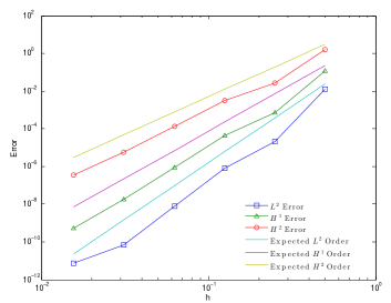
Figure 2. Test 1: orders of convergence in space for the full discretization of (26) with exact solution (94).

Test 2

For this test we take the exact solution to be

$$\psi(t;x,y)=\left[\left(1-\frac{x}{3}\right)\left(1-e^{-20\,x}\right)\sin(\pi y)\right]^{2}\sin(t)$$ (95)

with spatial domain $\Omega=[0,3]\times[0,1]$, which corresponds to Test 6 in [12] with a time-dependent term. The time interval for integration is $[0,0.5]$. A boundary layer will form along the western edge of the problem domain in this example. Note that the observed orders of convergence match the theoretical error estimates developed in Section 4. The results in Table 2 are also plotted in Figure 3.

$k$	$h$	DoFs	$e_{L^{2}}$	$L^{2}$ order	$e_{H^{1}}$	$H^{1}$ order	$e_{H^{2}}$	$H^{2}$ order
$\nicefrac{{1}}{{8192}}$	$\nicefrac{{1}}{{2}}$	$38$	$2.86\times 10^{-2}$	$-$	$5.16\times 10^{-1}$	$-$	$1.82\times 10^{1}$	$-$
$\nicefrac{{1}}{{8192}}$	$\nicefrac{{1}}{{4}}$	$174$	$4.79\times 10^{-3}$	$2.58$	$1.75\times 10^{-1}$	$1.56$	$9.28\times 10^{0}$	$0.973$
$\nicefrac{{1}}{{8192}}$	$\nicefrac{{1}}{{8}}$	$662$	$5.04\times 10^{-4}$	$3.25$	$3.38\times 10^{-2}$	$2.37$	$2.96\times 10^{0}$	$1.65$
$\nicefrac{{1}}{{8192}}$	$\nicefrac{{1}}{{16}}$	$2853$	$1.65\times 10^{-5}$	$4.94$	$2.17\times 10^{-3}$	$3.96$	$3.67\times 10^{-1}$	$3.01$
$\nicefrac{{1}}{{8192}}$	$\nicefrac{{1}}{{32}}$	$11690$	$4.17\times 10^{-7}$	$5.30$	$1.07\times 10^{-4}$	$4.34$	$3.47\times 10^{-2}$	$3.40$
$\nicefrac{{1}}{{8192}}$	$\nicefrac{{1}}{{64}}$	$47958$	$7.28\times 10^{-9}$	$5.84$	$3.70\times 10^{-6}$	$4.86$	$2.37\times 10^{-3}$	$3.87$

Table 2. Test 2: spatial orders of convergence with exact solution (95).

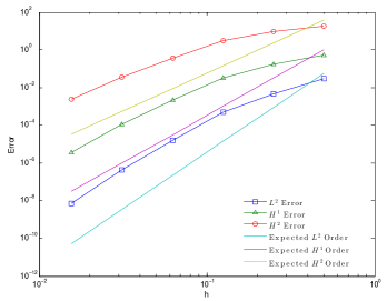
Figure 3. Test 2: orders of convergence in space for the full discretization of (26) with exact solution (95).

6. Conclusions

In this paper we studied the conforming FE semi-discretization of the pure streamfunction form of the QGE. This semi-discretization requires a $C^{1}$ FE, for which we chose the Argyris element. In Section 4 we developed rigorous error estimates for the conforming FE semi-discretization of the QGE. For this analysis only the fact that the semi-discretization is conforming was used. We showed that the orders of convergence are optimal.

Numerical experiments for the QGE (Section 5) with the Argyris element, were also carried out. The code which was developed and verified for the stationary QGE in [12] was then modified to deal with time-dependence. We applied an implicit Euler scheme and verified numerically the theoretical spatial rates of convergence developed for the semi-discretization.

The QGE have many unique challenges for numerical modeling. These challenges include (but are not limited to) unstable solutions, resulting from internal layers and western boundary layers, and high computational cost for large domains, such as the North Atlantic. To address these issues we plan to extend these studies in several directions to include stabilization methods. We are also interested in incorporating empirical wind-stress data, which will require parameter estimation techniques.

References

- [1] A. Adcroft and D. Marshall, How slippery are piecewise-constant coastlines in numerical ocean models?, Tellus, Ser. A and Ser. B-Dyn. Meteorol. Oceanogr., 50 (1998,), pp. 95–108.
- [2] D. Braess, Finite elements: Theory, fast solvers, and applications in solid mechanics, Cambridge University Press, 2001.
- [3] M. E. Cayco and R. A. Nicolaides, Finite element technique for optimal pressure recovery from stream function formulation of viscous flows, Math. of Comp., 46 (1986).
- [4] P. G. Ciarlet, The finite element method for elliptic problems, North-Holland, 1978.
- [5] B. Cushman-Roisin, Introduction to geophysical fluid dynamics, Prentice Hall, Englewood Cliffs, New Jersey, 1994.
- [6] B. Cushman-Roisin and J. M. Beckers, Introduction to geophysical fluid dynamics: Physical and numerical aspects, International Geophysics, Elsevier Science & Technology, 2011.
- [7] H. E. Dijkstra, Nonlinear physical oceanography: A dynamical systems approach to the large scale ocean circulation and el Nino, vol. 28, Springer Verlag, 2005.
- [8] F. Dupont, D. N. Straub, and C. A. Lin, Influence of a step-like coastline on the basin scale vorticity budget of mid-latitude gyre models, Tellus, Ser. A-Dyn Meteorol. Oceanogr., 55 (2003), pp. 255–272.
- [9] L. C. Evans, Partial Differential Equations, vol. 19, American Mathematical Society, Providence, 2010.
- [10] F. Fairag, A two-level finite-element discretization of the stream function form of the Navier-Stokes equations, Comp. Math. Applic., 36 (1998), pp. 117–127.
- [11] E. L. Foster, Finite Elements for the quasi-geostrophic equations of the ocean, PhD thesis, Virginia Polytechnic Institute and State University, 2013.
- [12] E. L. Foster, T. Iliescu, and Z. Wang, A finite element discretization of the streamfunction formulation of the stationary quasi-geostrophic equations of the ocean, Comp. Meth. Appl. Mech. and Eng., 261-262 (2013), pp. 105–117.
- [13] R. J. Greatbatch and B. T. Nadiga, Four-gyre circulation in a barotropic model with double-gyre wind forcing, J. Phys. Oceanogr., 30 (2000), pp. 1461–1471.
- [14] M. D. Gunzburger, Finite element methods for viscous incompressible flows, Computer Science and Scientific Computing, Academic Press Inc, 1989. A Guide to Theory, Practice, and Algorithms.
- [15] C. Johnson, Numerical solution of partial differential equations by the finite element method, vol. 32, Cambridge University Press, New York, 1987.
- [16] W. J. Layton, Introduction to the numerical analysis of incompressible viscous flows, vol. 6, Society for Industrial and Applied Mathematics (SIAM), 2008.
- [17] A. J. Majda and X. Wang, Non-linear dynamics and statistical theories for basic geophysical flows, Cambridge University Press, 2006.
- [18] J. Pedlosky, Geophysical fluid dynamics, Springer, second ed., 1992.
- [19] O. San, A. E. Staples, and T. Iliescu, Approximate deconvolution large eddy simulation of a barotropic ocean circulation model, Ocean Model., 40 (2011), pp. 120–132.
- [20] G. K. Vallis, Atmosphere and ocean fluid dynamics: Fundamentals and large-scale circulation, Cambridge University Press, 2006.
- [21] J. Wang and G. K. Vallis, Emergence of Fofonoff states in inviscid and viscous ocean circulation models, J. Mar. Res., 52 (1994), pp. 83–127.
- [22] Q. Wang, S. Danilov, and J. Schröter, Finite element ocean circulation model based on triangular prismatic elements, with application in studying the effect of topography representation, J. of Geophys. Res., 113 (2008).