Kahler: An Implementation of Discrete Exterior Calculus on Hermitian Manifolds

Abstract

This paper details the techniques and algorithms implemented in Kahler, a Python library that implements discrete exterior calculus on arbitrary Hermitian manifolds. Borrowing techniques and ideas first implemented in PyDEC, Kahler provides a uniquely general framework for computation using discrete exterior calculus. Manifolds can have arbitrary dimension, topology, bilinear Hermitian metrics, and embedding dimension. Kahler comes equipped with tools for generating triangular meshes in arbitrary dimensions with arbitrary topology. Kahler can also generate discrete sharp operators and implement de Rham maps. Computationally intensive tasks are automatically parallelized over the number of cores detected. The program itself is written in Cython–a superset of the Python language that is translated to C and compiled for extra speed. Kahler is applied to several example problems: normal modes of a vibrating membrane, electromagnetic resonance in a cavity, the quantum harmonic oscillator, and the Dirac-Kahler equation. Convergence is demonstrated on random meshes.

1 Introduction

The ideas and techniques used in Kahler are based on those pioneered by Bell and Hirani in PyDEC [2]. This section will briefly review the core concepts of discrete exterior calculus. Please refer to [3] for a more detailed overview of discrete exterior calculus, [2] for its implementation, and [1] for its continuous counterpart.

1.1 The Discrete Exterior Derivative

Each $p$-simplex, $\sigma^{p}$, is composed of $p+1$ vertices

$$\sigma^{p}=\left[v_{0},\dots,v_{p}\right]$$ (1.1)

In practice, only the indices of these vertices are stored in the simplices. The boundary of a $p$-simplex is defined as the formal sum of its $p-1$ dimensional faces [3]

$$\partial\sigma^{p}=\underset{i}{\sum}\left(-1\right)^{i}\left[v_{0},\dots,\hat{v_{i}}\dots,v_{p}\right]$$ (1.2)

The discrete exterior derivative is defined as the transpose of the boundary operator [3]

$$d=\partial^{T}$$ (1.3)

1.2 The Dual Mesh and the Hodge Star

The discrete Hodge star maps $p$-simplices, $\sigma^{p}=\left[v_{0},\dots,v_{p}\right]$ to their circumcentric duals [3]

$$\star\sigma^{p}=\underset{\sigma^{p+1}\prec\cdots\prec\sigma^{N}}{\sum}s\left(\sigma^{p},\dots,\sigma^{N}\right)\left[c\left(\sigma^{N}\right),\dots,c\left(\sigma^{p}\right)\right]$$ (1.4)

, where $c\left(\sigma\right)$ is the circumcenter of $\sigma$, $\sigma\prec\sigma^{\prime}$ means $\sigma$ is a face of $\sigma^{\prime}$. $s$ is $1$ when the orientation of $\left[c\left(\sigma^{N}\right),\dots,c\left(\sigma^{p}\right)\right]$ matches the orientation of $\left[\sigma^{N}\backslash\sigma^{N-1},\dots,\sigma^{p+1}\backslash\sigma^{p},c\left(\sigma^{p}\right)\right]$ and is $-1$ otherwise. The discrete Hodge star is then defined as the following diagonal matrix [3, 2]

$$\star_{ij}=\delta_{ij}\frac{\left|\star\sigma_{i}\right|}{\left|\sigma_{j}\right|}$$ (1.5)

where $\left|\sigma_{j}\right|$ is the primal volume of the $j^{\mathrm{th}}$ simplex and $\left|\star\sigma_{i}\right|$ is the volume of the dual cell of the $j^{\mathrm{th}}$ simplex. The codifferential is then defined as [3]

$$\delta_{p}=\left(-1\right)^{p}\star_{p-1}^{-1}d_{p-1}^{T}\star_{p}$$ (1.6)

2 Software Overview

2.1 Mesh Generation

For the purposes of this paper, mesh generation refers to converting a topological manifold to a set of $N$-simplices. Mesh generation is therefore separate from embedding the points that form these simplices in some subset of $\mathbb{C}^{M}$ with $M\geq N$. Kahler comes with tools that accomplish each of these tasks separately. This section is concerned with mesh generation.

2.1.1 Generating Simplicial Meshes in Arbitrary Dimensions

Kahler comes with two types of triangular mesh generators–one for asymmetric meshes and one for symmetric meshes as shown below.

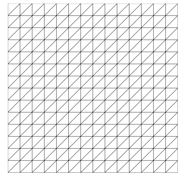
(a)

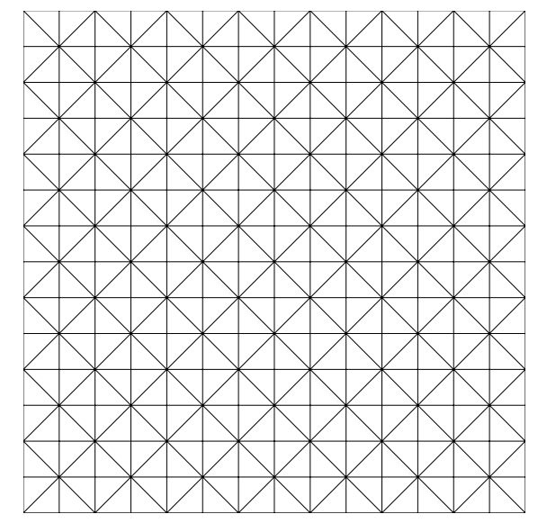
(b)

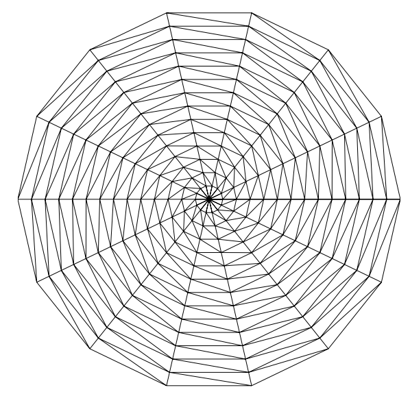
(c)

(d)

Figure 2.1: Asymmetric 2D mesh (top left), symmetric 2D mesh (top right), asymmetric polar mesh (bottom left), symmetric polar mesh (bottom right).

Similar meshes can be generated for tori, spheres, etc. Meshes start as an $M_{1}\times M_{2}\times\dots\times M_{N}$ grid of points created using the grid_indices() function. Grid indices are stored as dictionaries that map each index on the grid (grid index) to the corresponding index of the vertex (vertex index). Simplices are generated by connecting points to neighboring points. Simplices are stored as lists of vertex indices in the form of Numpy arrays. Asymmetric grids connect each point on the grid with a grid index of $\left[n_{1},\dots,n_{i},\dots n_{N}\right]$ to the point with grid index $\left[n_{1},\dots,n_{i}+1,\dots n_{N}\right]$. Symmetric grids connect every other point on the grid with a grid index of $\left[n_{1},\dots,n_{i},\dots n_{N}\right]$ to point with grid indices $\left[n_{1},\dots,n_{i}\pm 1,\dots n_{N}\right]$. Let $\vec{n}_{k}$ be the grid index of the $k^{\mathrm{th}}$ vertex in the simplex. Simplices are generated by constructing a series grid indices such that $\vec{n}_{k+1}-\vec{n}_{k}$ is a unit vector orthogonal to the plane formed by $\left[\vec{n}_{0},\dots,\vec{n}_{k}\right]$. In practice, only the vectors, $\vec{n}_{k}-\vec{n}_{0}$, are calculated. These vectors are added to each grid index and the original grid index dictionary is used to look up the corresponding vertex index–if it exists.

2.1.2 Customizing Topology

Once a list of simplices is created, arbitrary topologies can be created by joining one or more vertices together. For example, a torus is formed by joining vertices at opposite ends of the grid in question. This processes is hereby referred to as stitching. Stitches are stored as a dictionary that maps vertex indices to the corresponding vertex indices they are joined to. Kahler comes equipped with a function, pbc_stitches(), that will create the stitches necessary for periodic boundary conditions in one or more directions given a set of grid indices.

2.1.3 Singular Hodge Stars

The type of mesh discussed in this section creates right $N$-simplices. This means that the circumcenter of any $p$-simplex lies on its $p-1$ dimensional hypotenuse. The leads to dual cells with zero volume, which means that the inverse of the discrete Hodge star operator cannot be defined on those cells. This problem was remedied by adding a small but nonzero real number to each entry of the metric at each point. It is worth noting that this problem does not occure when calculating the Laplace-Beltrami operator for $0$-forms because the only dual volumes that need to be inverted are those of the $0$-simplices. These are generally nonzero even for right simplices.

2.2 The de Rham Map

A de Rham map is a mapping from a continuous differential form to a discrete one. Given a continuous $p$-form, $\alpha$, a de Rham map, $R$, is defined as follows

$$R:\alpha\Rightarrow\left(\sigma\rightarrow\int_{\sigma}\alpha\right)$$ (2.1)

where $\sigma$ is a $p$-simplex. When $\alpha$ is a continuous tensor field, the de Rham map is simply a zeroth order polynomial interpolation of $\alpha$ over the simplicial complex in question. Kahler uses a generalized trapezoidal rule to compute de Rham maps. Points are sampled evenly throughout the interior of each $N$-simplex. The interior of each $\left(N-k\right)$-face is given a weight of $1/2^{k}$.

2.3 Computing Circumcenters

Circumcenters are computed by solving a matrix equation. Given a (locally) flat Hermitian metric, $h$, a circumcenter can be defined as the linear combination of vertices, $c^{k}=\alpha^{I}v_{I}^{k}$, such that $\overline{\left(c^{j}-v_{I}^{j}\right)}h_{jk}\left(c^{k}-v_{I}^{k}\right)=\overline{\left(c^{j}-v_{0}^{j}\right)}h_{jk}\left(c^{k}-v_{0}^{k}\right)$ for each $1\leq I\leq p$, for a given $p$-simplex. Simplifying yields

$$2\Re\left(\overline{v}_{J}^{j}h_{jk}\left(v_{I}^{k}-v_{0}^{k}\right)\right)\alpha^{J}=\overline{v}_{I}^{j}h_{jk}v_{I}^{k}-\overline{v}_{0}^{j}h_{jk}v_{0}^{k}$$ (2.2)

This, combined with the constraint that $\sum\alpha^{I}=1$, uniquely determines the circumcenter.

2.4 Orienting Dual Volumes

Let the circumcenter of a $p$-simplex, $\sigma^{p}$ be $c\left(\sigma^{p}\right)$. A dual simplex of $\sigma^{p}$ is a simplex formed by $\left[c\left(\sigma^{N}\right),\dots,c\left(\sigma^{p}\right)\right]$ where $\sigma^{p}\prec\cdots\prec\sigma^{N}$. Let $V_{I}=c\left(\sigma^{p+I}\right)-c\left(\sigma^{p}\right)$ for $1\leq I\leq N$ and $\sigma^{p}\prec\cdots\prec\sigma^{p+I}\prec\cdots\prec\sigma^{N}$. Furthermore, let $U_{I}=\sigma^{p+I}\backslash\sigma^{p+I-1}-c\left(\sigma^{p}\right)$. Then the sign associated with a dual simplex, $\left[c\left(\sigma^{N}\right),\dots,c\left(\sigma^{p}\right)\right]$, is given by

$$\mathrm{sgn}\left(\Re\left(\det\left(\overline{V}^{i}h_{ij}U^{j}\right)\right)\right)$$ (2.3)

The metric, $h$, is the metric associated with $\sigma^{N}$.

2.5 Computing Barycentric Differentials

Barycentric differentials, $X$, are computed in a similar manner to the technique Bell and Hirani used for PyDEC. In Euclidean space [2]

$$X^{T}=\left(VV^{T}\right)^{-1}V$$ (2.4)

with $V_{I}^{i}=v_{I}^{i}-v_{0}^{i}$ for $I\in\left\{1,\dots,N\right\}$. This determines $N$ of the $N+1$ barycentric differentials. The last is determined from the constraint $\sum X^{I}=0$. In a space endowed with a Hermitian metric, $h$, this is easily modified accordingly.

$$X^{\dagger}=\left(V^{i}h_{ij}V^{\dagger j}\right)^{-1}V^{k}h_{kl}$$ (2.5)

2.6 The Discrete Sharp Operator

The discrete sharp operator maps discrete $p$-forms to antisymmetric tensors located at the barycenters of each $N$-simplex. Kahler wedges barycentric differentials to form antisymmetric tensors. The wedged differentials associated with each $p$-face of each $N$-simplex are averaged to give the tensor associated with the given $N$-simplex.

$$\alpha^{\sharp}\left(\sigma^{N}\right)=\frac{1}{A}\underset{i_{k},j=0}{\overset{N}{\sum}}\alpha\left(\left[\sigma_{i_{1}}^{N},\dots,\sigma_{i_{p}}^{N}\right]\right)\left(-1\right)^{j}d\lambda_{i_{1}}\wedge\dots\wedge\hat{d\lambda_{i_{j}}}\wedge\dots\wedge d\lambda_{i_{p}}$$ (2.6)

where $\sigma^{N}$ is an $N$-simplex, $\sigma_{i}^{N}$ is the $i^{\mathrm{th}}$ vertex of $\sigma^{N}$ such that $\left[\sigma_{i_{1}}^{N},\dots,\sigma_{i_{p}}^{N}\right]$ forms a $p$-simplex. $d\lambda_{i}$ is the $i^{\mathrm{th}}$ barycentric differential at $\sigma^{N}$. $A$ is the total number of terms in the sum, given by $A={n+1\choose p+1}{p+1\choose p}=\frac{\left(n+1\right)!}{p!\left(n+1-p\right)!}$. In practice, the discrete sharp operator is stored as a compressed matrix for speed and memory efficiency. When it is dotted with a $p$-form, it gives a flattened list of antisymmetric tensors. That is, the result is a one dimensional array that can be reshaped into a list of the desired antisymmetric tensors.

3 Examples

3.1 Normal Modes of a Vibrating Membrane

A vibrating membrane can be modeled as a scalar field, $\phi$, that satisfies the condition $-\delta d\phi=\lambda\phi$. When the membrane is held taught at the boundary, it obeys the Dirichlet condition $\phi=0$ at the boundary. When the membrane is allowed to vibrate freely at the boundary (as is the case for a Chladni plate), $\delta\phi=0$ at the boundary. Operating $\delta$ on both sides of the original eigenvalue equation and making use of $\delta^{2}=0$ yields $-\delta\delta d\phi=0=\delta\lambda\phi$. So this condition is automatically satisfied by solving the eigenvalue problem with the usual Laplace-Beltrami operator.

In each case, a $20\times 20$ grid was used over the interval $\left[0,\pi\right]\times\left[0,\pi\right]$. For visualization, the discrete $0$-forms were sharpened and interpolated over a fine grid.

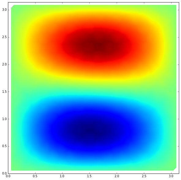
(a)

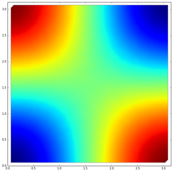
(b)

Figure 3.1: The third normal mode of a drum with Dirichlet boundary conditions (left) and Neumann boundary conditions (right).

Analytic	Numerical	%Error
2	1.99	0.426
5	4.95	1.03
5	4.95	0.914
8	7.91	1.11
10	9.80	2.05
10	9.80	2.05
13	12.8	1.95
13	12.8	1.82
17	16.4	3.59
17	16.4	3.58

Table 3.1: The First 10 eigenfrequencies of a drum with Dirichlet boundary conditions.

Analytic	Numerical	%Error
1	0.99	0.587
1	1.00	0.266
2	1.99	0.427
4	3.96	1.11
4	3.96	1.11
5	4.95	1.09
5	4.96	0.851
8	7.91	1.11
9	8.80	2.25
9	8.80	2.21

Table 3.2: The first 10 eigenfrequencies mode of a square drum with Neumann boundary conditions.

3.2 Electromagnetic Resonance in a Cavity

Electromagnetic waves in a cavity can be written in terms of the electric field, $\vec{E}$, or the magnetizing field, $\vec{H}$ [4]. The governing equations are the same for both, but the boundary conditions are different. The electric field obeys the Dirichlet condition that at the boundary, the component of $\vec{E}$ parallel to the boundary is zero. Let $E=\vec{E}^{\flat}$ and $H=\vec{H}^{\flat}$. When read in terms of differential forms, $E=0$ at the boundary. At the boundary, the $\vec{H}$ field is zero perpendicular to the boundary. When read in terms of differential forms, $\delta H=0$ at the boundary. Since $\delta dH=\lambda H$, operating with the codifferential on both sides and making use of $\delta^{2}=0$ yields $\delta\delta dH=0=\delta\lambda H$. So this condition is automatically satisfied by solving the eigenvalue problem with the usual Laplace-Beltrami operator.

In each case, a $20\times 20$ grid was used over the interval $\left[0,\pi\right]\times\left[0,\pi\right]$. For visualization, the discrete $1$-forms were sharpened and interpolated over a fine grid.

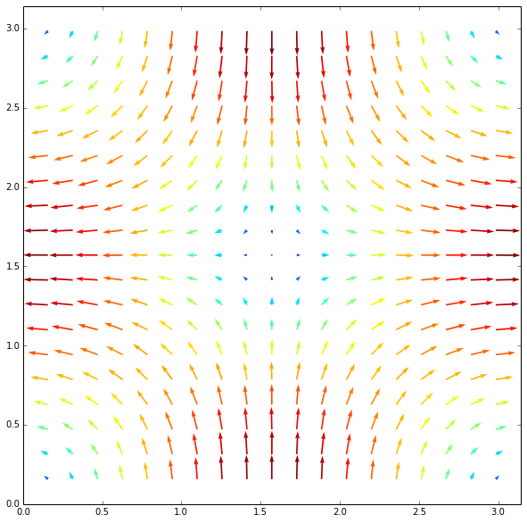
(a)

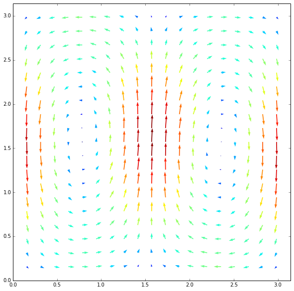
(b)

Figure 3.2: The third normal mode of electric field (left) and magnetic field (right) in a resonant cavity.

Analytic	Numerical	%Error
1	0.996	0.386
1	1.00	0.080
2	2.00	0.233
4	3.96	1.06
4	3.97	0.763
5	4.96	0.869
5	4.97	0.685
8	7.93	0.913
9	8.80	2.19
9	8.83	1.89

Table 3.3: The first 10 eigenfrequencies of an electric field in a resonant cavity.

Analytic	Numerical	%Error
2	2.00	0.233
5	4.96	0.868
5	4.97	0.687
8	7.93	0.913
10	9.80	1.98
10	9.83	1.74
13	12.8	1.75
13	12.8	1.64
17	16.4	3.53
17	16.4	3.27

Table 3.4: The first 10 eigenfrequencies of a of magnetic field in a resonant cavity.

3.3 The Quantum Harmonic Oscillator

An $M\times\dots\times M$ asymmetric Cartesian grid was used to solve the quantum harmonic oscillator problem [6].

$$\frac{1}{2}\nabla^{2}\psi+\frac{1}{2}x^{2}\psi=E\psi$$ (3.1)

A de Rham map was used to map the potential to the barycenters of the $N$-simplices. Call this representation of the potential $V^{\sharp}$. A least squares fit was used to derive the $0$-form representation of the potential, $V$ (effectively inverting the sharp operator for $0$-forms).

One Dimension

A $20$ point grid on the interval $\left[-\pi,\pi\right]$ was used for the one dimensional harmonic oscillator.

Analytic	Numerical	%Error
0.5	0.483	3.37
1.5	1.47	1.80
2.5	2.47	1.35
3.5	3.49	0.164
4.5	4.60	2.19
5.5	5.81	5.64
6.5	7.13	9.73
7.5	8.55	14.1
8.5	10.0	17.8
9.5	11.5	21.3

Table 3.5: The first 10 eigenfrequencies of a one dimensional quantum harmonic oscillator.

Two Dimensions

A $20\times 20$ point grid on the interval $\left[-\pi,\pi\right]\times\left[-\pi,\pi\right]$ was used for the two dimensional harmonic oscillator.

Analytic	Numerical	%Error
1	0.97	2.76
2	1.96	1.89
2	1.96	1.89
3	2.95	1.60
3	2.96	1.48
3	2.96	1.481
4	3.95	1.37
4	3.95	1.365
4	3.98	0.407
4	3.98	0.407

Table 3.6: The first 10 eigenfrequencies of a two dimensional quantum harmonic oscillator.

Three Dimensions

A $20\times 20\times 20$ point grid on the interval $\left[-\pi,\pi\right]\times\left[-\pi,\pi\right]\times\left[-\pi,\pi\right]$ was used for the three dimensional harmonic oscillator.

Analytic	Numerical	%Error
1.5	1.46	2.45
2.5	2.45	1.88
2.5	2.45	1.88
2.5	2.45	1.88
3.5	3.44	1.63
3.5	3.44	1.63
3.5	3.44	1.63
3.5	3.45	1.53
3.5	3.45	1.53
3.5	3.45	1.53

Table 3.7: The first 10 eigenfrequencies of a three dimensional quantum harmonic oscillator.

3.4 The Dirac-Kahler Equation

The Dirac-Kahler operator, $d+\delta$, operates on a formal sum of differential forms of different dimension [5]. A $20\times 20$ point grid on the interval $\left[0,\pi\right]\times\left[0,\pi\right]$ was used for the two dimensional Dirac-Kahler equation with a Euclidean metric. Dirichlet boundary conditions were applied to each of the three $p$-forms.

Analytic	Numerical	%Error
1	0.997	0.272
1	0.999	0.104
1.41	1.41	0.189
2	1.99	0.554
2	1.99	0.503
2.24	2.22	0.523
2.24	2.23	0.400
2.28	2.81	0.530
3	2.97	1.13
3	2.97	1.07

Table 3.8: The first 10 eigenvalues of the two dimensional Dirac-Kahler operator with a Euclidean metric.

3.5 Random Meshes

Some care must be taken when generating random meshes. Points cannot be too close or the resulting simplices will have zero volume. Furthermore, if an $N$ dimensional rectangular domain is to be covered randomly, all $p$ dimensional planes must also contain at least one point. The first requirement was satisfied by resampling points until all points were no closer than a cutoff distance, $R$. The second requirement can be satisfied by breaking up the point sampling into sampling at all corners, then all lines, two dimensional faces, etc. All the while, points are resampled until none are closer than $R$ to each other and all previously sampled points. In practice, $R=\frac{1}{2}\frac{1}{M^{1/N}}$, where $M$ is the number of points on the mesh. Finally, the resulting points are Delaunay triangulated. Kahler comes with a function, random_mesh(), that can create arbitrary dimensional random meshes with periodicity in an any number and combination of directions. For testing purposes, a two dimensional mesh was generated for different numbers of points

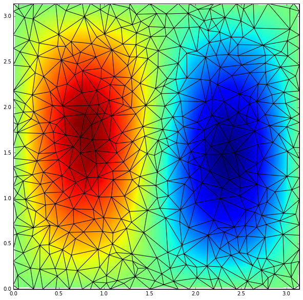
(a)

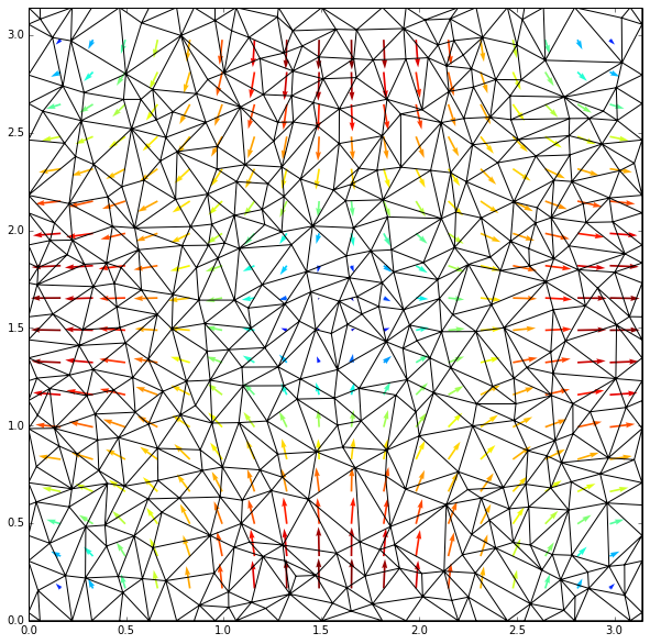
(b)

Figure 3.3: The third normal mode of vibrating drum with Dirichlet boundary conditions (left) and electric field (right) in a resonant cavity.

Analytic	Numerical	%Error
2	1.99	0.391
5	4.95	1.04
5	4.97	0.598
8	7.86	1.76
10	9.78	2.16
10	9.85	1.48
13	12.6	3.29
13	12.7	2.44
17	16.3	3.83
17	16.4	3.41

Table 3.9: The first 10 eigenfrequencies of a vibrating drum with Dirichlet boundary conditions.

Analytic	Numerical	%Error
1	0.99	0.245
1	1.00	0.178
2	1.99	0.466
4	3.96	0.778
4	3.96	0.518
5	4.95	1.37
5	4.96	0.858
8	7.91	1.19
9	8.80	1.48
9	8.80	0.989

Table 3.10: The first 10 eigenfrequencies of an electric field in a resonant cavity.

3.6 Convergence

Convergence was analyzed for square membrane with Dirichlet boundary conditions on a random mesh. The average percent error of the first 10 eigenfrequencies of this membrane was computed for increasing numbers of vertices. The results were repeated five times and averaged.

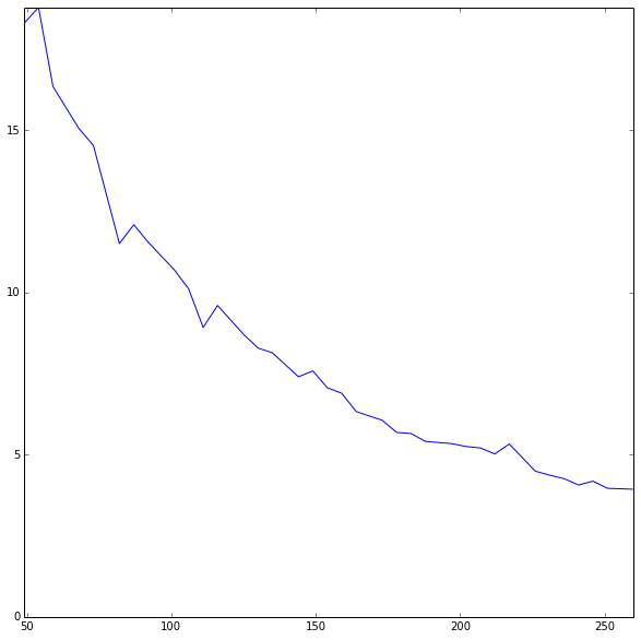
Figure 3.4: The mean of percent errors of the first 10 eigenfrequencies of a square membrane with Dirichlet boundary conditions vs the number of points on a random mesh.

References

- [1] R Abraham. Manifolds, Tensor Analysis, and Applications. Number March 2007. 1988.
- [2] Nathan Bell and AN Hirani. PyDEC : Software and Algorithms for Discretization of Exterior Calculus. ACM Transactions on Mathematical Software (TOMS), pages 1–39, 2012.
- [3] AN Hirani. Discrete exterior calculus. pages 1–53, 2005.
- [4] J D Jackson. Classical electrodynamics. Wiley, 1975.
- [5] V. M. Red’kov. Dirac-Kahler equation in curved space-time, relation between spinor and tensor formulations. page 20, September 2011.
- [6] R Shankar. Principles of quantum mechanics. 1994.