Quantum theory of the Bianchi II model

Abstract

We describe the quantum evolution of the vacuum Bianchi II universe in terms of the transition amplitude between two asymptotic quantum Kasner-like states. For large values of the momentum variable the classical and quantum calculations give similar results. The difference occurs for small values of this variable due to the Heisenberg uncertainty principle. Our results can be used, to some extent, as a building block of the quantum evolution of the vacuum Bianchi IX universe.

I Introduction

In cosmology, almost all known general relativity (GR) models of the Universe predict the existence of cosmological singularities with blowing up gravitational and matter field invariants. These singularities indicate the breakdown of classical theory at extreme physical conditions. The existence of the cosmological singularities in solutions to GR signals incompleteness of the classical theory. It is expected that a consistent theory of quantum gravity should resolve the classical singularities.

The Belinskii-Khalatnikov-Lifshitz (BKL) scenario BKL22 ; BKL33 is thought to be a generic solution to the Einstein equations near spacelike singularity. It has been proved that the isotropy of spacetime is dynamically unstable in the evolution towards the singularity (see, e.g. BKL22 ; Bogo ). Therefore, it seems that the commonly used Friedmann-Robertson-Walker (FRW) model cannot be used to model the very early Universe. The prototype for the BKL scenario is the vacuum Bianchi IX model BKL22 . The building blocks of this model are the vacuum Bianchi I and II models BKL22 ; Reiterer:2010cz . We expect that obtaining quantum versions of the latter models may be helpful in the quantization of the former one. The quantum Bianchi IX model may enable finding the nonsingular quantum BKL theory, which could be used as a realistic model of the very early Universe.

The quantization of the Bianchi I, II, and IX models with the aim of resolving the classical singularity problem has already been proposed within the loop quantization approach Ashtekar:2009vc ; Ashtekar:2009um ; WilsonEwing:2010rh . Our investigations of the quantum Bianchi I model, based on a modification of the latter method, can be found in DzP ; MPDz ; Malkiewicz:2011sr . The goal of the present article is quite different. Namely, we treat the Bianchi II as a model of a single transition between two consecutive Kasner’s epochs of the Bianchi IX dynamics only. It is not expected to be valid at the cosmological singularity. The quantization of some anisotropic cosmological models has been explored before (see, e.g., TCh ; JEL ), but mostly within the Dirac approach. Our procedure involves a reduction of the dynamical constraint at the classical level, followed by quantization of true Hamiltonian.

In Sec. II we first present the Misner-like canonical formulation of our homogeneous models. In this approach, the Universe is interpreted to be a “particle” with its mass depending on time and position in space cwm1 ; cwm2 . Next, we find dynamical interrelations between both classical Bianchi models. The quantum level is presented in Sec. III. We solve the Schrödinger equation for the Bianchi II model. The solution is interpreted in terms of the “scattering” of the Kasner universe against the potential wall of the Bianchi II universe. The asymptotic form of the solution enables determination of the scattering amplitude. In the last section we suggest that our results can be used, to some extent, as a building block of the evolution of the Bianchi IX model.

II Classical dynamics

We assume spacetime admitting a foliation $\mathcal{M}\mapsto\Sigma\times\mathbb{R}$, where $\Sigma$ is spacelike. The line element of the spatially homogenous, diagonal Bianchi models reads

$$\mathrm{d}s^{2}=-N(t)^{2}\mathrm{d}t^{2}+\sum_{i}q_{i}(t){\omega^{i}}\otimes{\omega^{i}}\,,$$ (1)

where $\omega^{i}$ are 1-forms on $\Sigma$ invariant with respect to the action of a simply transitive group of motions on the leaf and subject to

$$\mathrm{d}\omega^{i}=\frac{1}{2}C^{i}_{jk}\omega^{j}\wedge\omega^{k}\,,$$ (2)

where $C^{i}_{jk}$ are structure constants of the corresponding Lie algebra. In the case of the Bianchi I model one has $C^{i}_{jk}=0$ for any $i,j,k$. The Bianchi II model is specified by the only nonvanishing $C^{1}_{23}=-C^{1}_{32}=n_{1}\neq 0$. One can choose $n_{1}>0$, and its value is usually fixed by the condition $n_{1}=1$. In what follows we keep $n_{1}$ as a parameter. A solution to (2) reads

$$\omega^{1}=dx-n_{1}zdy,~{}~{}\omega^{2}=dy,~{}~{}\omega^{3}=dz,$$ (3)

where $x$, $y$ and $z$ are coordinates on $\Sigma$.

We recall that in canonical relativity there are the so-called diffeomorphism constraints, which are first class and generate canonical transformations, whose action geometrically corresponds to spatial diffeomorphisms in space-time. Those diffeomorphisms are viewed as coordinate transformations and, as such, are unphysical. The gauge-fixing procedure may be applied to extract the physical degrees of freedom HT . The diffeomorphism constraints, however, are absent in our model because of the spatial homogeneity, which allowed us to fix the metric in the form of Eq. (1). Nevertheless, there are still some restricted (homogeneous) transformations of $\omega^{i}$’s so the gauge is not fixed completely and we need to fix it further.

Let $\tilde{\omega}^{1}$, $\tilde{\omega}^{2}$ and $\tilde{\omega}^{3}$ be another solution of (2). Then, because the old and the new solutions are invariant with respect to the action of the same homogeneity group, they must be related by a linear transformation $L^{i}_{~{}j}$ such that

$$\tilde{\omega}^{i}=L^{i}_{~{}j}\omega^{j},~{}~{}~{}(L^{i^{\prime}}_{~{}i})^{-1}C^{i}_{jk}L^{j}_{~{}j^{\prime}}L^{k}_{~{}k^{\prime}}=C^{i^{\prime}}_{j^{\prime}k^{\prime}}.$$ (4)

This implies in particular that $d\tilde{\omega}^{2}=0=d\tilde{\omega}^{3}$. Thus, $L^{2}_{~{}1}=0=L^{3}_{~{}1}$, and

$$\tilde{\omega}^{2}=L^{2}_{~{}2}\omega^{2}+L^{2}_{~{}3}\omega^{3},~{}~{}~{}\tilde{\omega}^{3}=L^{3}_{~{}2}\omega^{2}+L^{3}_{~{}3}\omega^{3},$$ (5)

We set $\Lambda:=L^{2}_{~{}2}L^{3}_{~{}3}-L^{2}_{~{}3}L^{3}_{~{}2}\neq 0$. From it easily follows that

$$d\tilde{\omega}^{1}=\tilde{\omega}^{2}\wedge\tilde{\omega}^{3}=\Lambda{\omega}^{2}\wedge{\omega}^{3}=\Lambda d\omega^{1}~{}~{}\Rightarrow\tilde{\omega}^{1}=\Lambda{\omega}^{1}+L^{1}_{~{}2}\omega^{2}+L^{1}_{~{}3}\omega^{3}.$$ (6)

Thus, at the level of coordinates, the possible transformation (up to a constant shift) is the following

$$\tilde{x}=\Lambda x,~{}~{}\tilde{y}=L^{2}_{~{}2}y+L^{2}_{~{}3}z,~{}\tilde{z}=L^{3}_{~{}2}y+L^{3}_{~{}3}z.$$ (7)

However, when combined with the requirement that $L^{i}_{~{}j}$ preserves the form of the metric (1), that is

$$\sum_{i}q_{i}(t){\omega^{i}}\otimes{\omega^{i}}=\sum_{i}\tilde{q}_{i}(t){\tilde{\omega}^{i}}\otimes{\tilde{\omega}^{i}}$$ (8)

we find that $L^{2}_{~{}3}=0=L^{3}_{~{}2}$. Now, we demand that $x$ and $y$ be coordinates on a compact manifold, say $\mathbb{T}^{2}$, such that $\int_{\mathbb{S}}dx=\int_{\mathbb{S}}dy=1$, while $z\in\mathbb{R}$. This fixes the 1-forms completely and restricts the allowed coordinate transformations as follows:

$$\tilde{x}=x+x_{0},~{}~{}\tilde{y}=y+y_{0},~{}\tilde{z}=z+z_{0},$$ (9)

Thus, the variables $q_{i}$ are now physical.

We assume a fiducial cell which is the Cartesian product of the whole $\mathbb{T}^{2}$ and any compact subset $\sigma_{z}\subset\mathbb{R}$. The following holds:

$$\int_{\mathbb{T}^{2}\times\sigma_{\tilde{z}}}d\tilde{x}\wedge d\tilde{y}\wedge d\tilde{z}=\int_{\mathbb{T}^{2}\times\sigma_{z}}dx\wedge dy\wedge dz$$ (10)

so even if the variable $z$ may be chosen only up to a shift, the volume of the patch is uniquely defined. We believe that having a well-defined volume of the fiducial cell is essential for having physically meaningful variables in the case of spatially homogeneous and noncompact universes.

Due to the homogeneity of the space, the action of the vacuum Bianchi I and II models takes the general form

$$S=\frac{1}{\kappa}\int_{\mathcal{V}\subset\Sigma}\,\eta\,\int NL(q_{i},\frac{\dot{q}_{i}}{N})\,dt=\frac{\Delta}{\kappa}\int N\,dt\,L(q_{i},\frac{\dot{q}_{i}}{N})\;,$$ (11)

where (i) $N$ is the lapse function, $L$ is the Lagrangian function of $(q_{i},\dot{q}_{i})$ and $\kappa=8\pi G$, (ii) $\eta$ is the 3-form $\eta=\omega_{1}\wedge\omega_{2}\wedge\omega_{3}$. $\mathcal{V}$ denotes a finite patch in $\Sigma$, over which the integration is performed. $\Delta=\int_{\mathcal{V}\subset\Sigma}\eta$ will be the fiducial volume in $\Sigma$.

Therefore the models only depend on the effective gravitational constant $\tilde{\kappa}=\kappa/\Delta$. The Hamiltonians read Bogo

$$H=\frac{1}{\tilde{\kappa}}\frac{N}{\sqrt{q_{1}q_{2}q_{3}}}\bigg{(}-q_{1}^{2}p_{1}^{2}-q_{2}^{2}p_{2}^{2}-q_{3}^{2}p_{3}^{2}+2\big{(}q_{1}p_{1}q_{2}p_{2}+q_{1}p_{1}q_{3}p_{3}+q_{2}p_{2}q_{3}p_{3}\big{)}-\frac{1}{4}n_{1}^{2}q_{1}^{2}\bigg{)}$$ (12)

where $p_{k}$ denotes the conjugate momentum variable to $q_{k}$, according to the Poisson bracket $\{q_{i},p_{j}\}=\tilde{\kappa}\,\delta_{ij}$. Also, $n_{1}=0$ and $n_{1}\neq 0$ correspond to the Bianchi I and Bianchi II models, respectively. Note that the dimension of $\tilde{\kappa}$ reads $[\tilde{\kappa}]=action^{-1}length^{-1}$, and assuming the $q_{i}$ variables to be dimensionless, the dimensions of $p_{i}$ and $n_{1}$ are $[p_{i}]=[n_{1}]=length^{-1}$.

Both systems have the dynamical constraint $H=0$. The case of vanishing of the physical volume of the patch, $\,V:=\Delta\cdot\sqrt{q_{1}q_{2}q_{3}}=0\,$, defines the condition for the appearance of the cosmological singularity Bogo . Our paper does not address the singularity problem so the expression (12) is well defined. Our considerations concern the evolution towards the singularity excluding the singularity itself. We study possible quantum effects before physical quantities reach their critical values, at which the big bounce is expected to take place. The classical model, Bianchi II, is assumed to be valid only as a model of a single transition between two successive Kasner’s universes, i.e., a patch of the evolution towards the singularity, and is not meant to be a model of the classical dynamics near the singularity. This is the reason for our placing the singularity at infinity and emphasizing the scattering picture at the quantum level. As the result, our findings are limited to a single event of the quantum evolution: the quantum transition between two Kasner’s epochs.

It is not difficult to relate the canonical approaches developed independently by Bogoyavlensky, presented in his textbook Bogo , and by Misner cwm1 ; cwm2 ; RS . The latter one has been commonly used for about four decades. The former is a comprehensive analysis of the classical dynamics of all homogeneous models carried out within one formalism.

For further analysis we introduce Misner’s like three canonical pairs $(\beta_{0},\pi_{0},\beta_{\pm},\pi_{\pm})$ as follows

$$\beta_{0}:=\ln{(q_{1}\sqrt{q_{2}q_{3}})},~{}~{}~{}\beta_{+}:=\ln q_{1},~{}~{}~{}\beta_{-}:=\ln{\sqrt{q_{2}/q_{3}}}$$ (13)

$$\pi_{0}:=q_{2}p_{2}+q_{3}p_{3},~{}~{}~{}\pi_{+}:=q_{1}p_{1}-q_{2}p_{2}-q_{3}p_{3},~{}~{}~{}\pi_{-}:=q_{2}p_{2}-q_{3}p_{3}$$ (14)

One easily verifies that $\{\beta_{i},\pi_{j}\}=\tilde{\kappa}\,\delta_{ij}$. The Hamiltonian (12) in these new variables has the form

$$H=Ne^{-(\beta_{0}-\frac{1}{2}\beta_{+})}\Big{(}\pi_{0}^{2}-\pi_{+}^{2}-\pi_{-}^{2}-\frac{n_{1}^{2}}{4}e^{2\beta_{+}}\Big{)}.$$ (15)

We note that $\pi_{0}$ is a dynamical constant and that the sign of $\pi_{0}$ corresponds to the direction of evolution. We will use this fact to define the true Hamiltonian of the system(s).

II.1 True Hamiltonian

The canonical 2-form $\omega$ that can be ascribed to the six-dimensional kinematical phase space of our system reads

$$\tilde{\kappa}\cdot\omega=\mathrm{d}\pi_{+}\wedge\mathrm{d}\beta_{+}+\mathrm{d}\pi_{-}\wedge\mathrm{d}\beta_{-}+\mathrm{d}\pi_{0}\wedge\mathrm{d}\beta_{0}.$$ (16)

We restrict $\pi_{0}>0$ and introduce the new canonical pair

$$\beta_{0}^{\prime}=-\frac{\beta_{0}}{2\pi_{0}},~{}~{}\pi_{0}^{\prime}=-\pi_{0}^{2}$$ (17)

Reduction of the form (16) to constraint surface $H=0$ leads to

$$\tilde{\kappa}\cdot\omega|_{H=0}=\mathrm{d}\pi_{+}\wedge\mathrm{d}\beta_{+}+\mathrm{d}\pi_{-}\wedge\mathrm{d}\beta_{-}-\mathrm{d}h\wedge\mathrm{d}\beta_{0}^{\prime},$$ (18)

where

$$h=\pi_{+}^{2}+\pi_{-}^{2}+\frac{n_{1}^{2}}{4}e^{2\beta_{+}}$$ (19)

is the true Hamiltonian in the reduced formulation. Thus, as one may verify that the following is satisfied:

$$\frac{\mathrm{d}\beta_{\pm}}{\mathrm{d}\beta_{0}^{\prime}}=\frac{\partial h}{\partial\pi_{\pm}},~{}~{}~{}~{}\frac{\mathrm{d}\pi_{\pm}}{\mathrm{d}\beta_{0}^{\prime}}=-\frac{\partial h}{\partial\beta_{\pm}}.$$ (20)

Therefore, we have the Hamiltonian system defined in the physical phase space with $h$ being the generator of motion and $\beta_{0}^{\prime}$ playing the role of time. Note that the direction of evolution is set by the growth of $\beta_{0}^{\prime}$, which corresponds to the contraction of universe. Furthermore, by the virtue of Eq. (20), the classical dynamics is invariant with respect to the choice of the fiducial cell $\mathcal{V}$ in $\Sigma$.

II.2 Bianchi I as the asymptotic past/future of Bianchi II

In what follows we find dynamical relation between the two Bianchi models. This has already been done (see, e.g. Bogo ), to some extent, but within different parametrization of phase space and in different context. Here, we use Misner’s like variables, which are convenient in our quantization procedure. This way we obtain the consistency between classical and quantum levels.

Equations (20) read explicitly

$$\dot{\beta}_{+}=2\pi_{+},~{}~{}~{}\dot{\beta}_{-}=2\pi_{-},$$ (21)

$$\dot{\pi}_{+}=-\frac{n_{1}^{2}}{2}e^{2\beta_{+}},~{}~{}~{}\dot{\pi}_{-}=0.$$ (22)

The system (21)-(22) integrates easily for the Bianchi II case ($n_{1}\neq 0$) to the form

$$\beta_{+}=\ln{\left[\operatorname{sech}{\left(a_{1}\beta_{0}^{\prime}+a_{2}\right)}\right]}+\ln\frac{a_{1}}{n_{1}},~{}~{}~{}\beta_{-}=a_{3}\beta_{0}^{\prime}+a_{4},$$ (23)

$$\pi_{+}=-\frac{a_{1}}{2}\tanh\left(a_{1}\beta_{0}^{\prime}+a_{2}\right),~{}~{}~{}\pi_{-}=\frac{a_{3}}{2},$$ (24)

where $a_{1},a_{2},a_{3},a_{4}$ are real constants, $a_{1}>0$. It is clear that the dimension of $a_{1}$ and $a_{3}$ is an action (the inverse of the dimension of $\beta_{0}^{\prime}$). The remaining constants are dimensionless. Asymptotically, as $\beta_{0}^{\prime}\rightarrow\pm\infty$, we obtain $\beta_{+}\rightarrow-\infty$ and $\pi_{+}\rightarrow\mp\frac{a_{1}}{2}$. Another way of obtaining this result is realizing that (21)-(22) imply

$$\ddot{\beta}_{+}=-(n_{1}e^{\beta_{+}})^{2}<0,~{}~{}~{}\beta_{0}^{\prime}\in\mathbb{R},$$ (25)

which means that the graph of $\beta_{+}$ is globally concave. Consequently, $\beta_{+}\rightarrow-\infty$, as $\beta_{0}^{\prime}\rightarrow\pm\infty$, which is the key in showing the asymptotic equivalence of the two Bianchi models.

In the case of the Bianchi I model ($n_{1}=0$), Eqs. (20) read explicitly

$$\dot{\beta}_{+}=2\pi_{+},~{}~{}~{}\dot{\beta}_{-}=2\pi_{-},$$ (26)

$$\dot{\pi}_{+}=0,~{}~{}~{}\dot{\pi}_{-}=0,$$ (27)

and have the obvious solution

$$\beta_{+}=b_{1}\beta_{0}^{\prime}+b_{2},~{}~{}~{}\beta_{-}=b_{3}\beta_{0}^{\prime}+b_{4},$$ (28)

$$\pi_{+}=\frac{b_{1}}{2},~{}~{}~{}\pi_{-}=\frac{b_{3}}{2},$$ (29)

where $b_{1},b_{2},b_{3},b_{4}$ are real constants. We note that the Bianchi II solution (23-(24) for large $\pm\beta_{0}^{\prime}$ coincides with the Bianchi I solutions (28-(29) with

$$b_{1}=\mp a_{1},~{}~{}b_{2}=\ln\frac{a_{1}}{n_{1}}\mp a_{2},~{}~{}b_{3}=a_{3},~{}~{}b_{4}=a_{4}\,.$$ (30)

Therefore, we have explicitly shown that asymptotically, as time goes to $\pm\infty$, the solutions of the two Bianchi models coincide.

II.3 An energy-dependent wall approximation for Bianchi-II

Using Eqs. (23) and (24) and introducing the definition $\pi_{+}^{\infty}=a_{1}/2>0$ for the asymptotic value of $\pi_{+}$ at $\beta_{0}^{\prime}\to-\infty$, we see that the trajectory (qualitatively) looks like a reflection on an infinite wall. The position of the wall can be obtained from the turning point of the trajectory $\dot{\beta_{+}}=2\pi_{+}=0$. We deduce from (24) that $\beta_{0}^{\prime}=-a_{2}/a_{1}=-2a_{2}/\pi_{+}^{\infty}$, and the corresponding value $\beta_{+}^{(C)}$ of $\beta_{+}$, due to (23), reads

$$\beta_{+}^{(C)}=\ln\frac{a_{1}}{n_{1}}=\ln\frac{2\pi_{+}^{\infty}}{n_{1}}\,.$$ (31)

Thus, the main features of the trajectories can be grasped via introducing an infinite wall approximation with the position $\beta_{+}^{(C)}$ of the wall being $\pi_{+}^{\infty}$ dependent. As will be seen later, the quantum version of the model completely modifies the position $\beta_{+}^{(C)}$ of the wall for small values of $\pi_{+}^{\infty}$.

III Quantum dynamics

In what follows we apply the canonical quantization method. The variables of the physical phase space satisfy

$$\{\beta_{+},\pi_{+}\}=\tilde{\kappa}=\{\beta_{-},\pi_{-}\},$$ (32)

with vanishing other Poisson bracket relations (for simplicity we use here the same notation for the Poisson bracket as in the preceding section). To quantize the algebra (32) we apply the Schrödinger representation

$$\beta_{\pm}\rightarrow\hat{\beta}_{\pm}f(\beta_{+},\beta_{-}):=\beta_{\pm}f(\beta_{+},\beta_{-}),~{}~{}~{}\pi_{\pm}\rightarrow\hat{\pi}_{\pm}f(\beta_{+},\beta_{-}):=-i\hbar_{b}\frac{\partial}{\partial\beta_{\pm}}f(\beta_{+},\beta_{-}),$$ (33)

where $f\in\mathcal{H}:=L^{2}(\mathbb{R}^{2},d\beta_{+}d\beta_{-})$ and $\hbar_{b}=\tilde{\kappa}\hbar$ corresponds to the action constant relevant in our case. In the following calculations we set $\hbar_{b}=1$ to simplify expressions.

The quantum operator $\hat{h}$ corresponding to the classical Hamiltonian $h$ of Eq. (19) reads

$$\hat{h}=\hat{\pi}_{+}^{2}+\hat{\pi}_{-}^{2}+\frac{n_{1}^{2}}{4}e^{2\hat{\beta}_{+}}.$$ (34)

Since the Hamiltonian $\hat{h}$ is time independent, the stationary solution to the Schrödinger equation

$$i\frac{\partial}{\partial\beta_{0}^{\prime}}\Psi=\hat{h}\;\Psi$$ (35)

can be written in the form $\Psi_{E}(\beta_{0}^{\prime},\beta_{-},\beta_{+})=e^{-iE\beta_{0}^{\prime}}\psi_{E}(\beta_{-},\beta_{+})$, with $E>0$, where

$$\hat{h}\psi_{E}=E\psi_{E}.$$ (36)

Therefore, the problem reduces to the problem of solving the eigen equation (36).

III.1 The generalized eigenvectors of Hamiltonian $\hat{h}$

We have

$$\hat{h}=\hat{h}_{-}+\hat{h}_{+},$$ (37)

where

$$\hat{h}_{-}=-\frac{\partial^{2}}{\partial\beta^{2}_{-}},~{}~{}~{}\hat{h}_{+}=-\frac{\partial^{2}}{\partial\beta^{2}_{+}}+\frac{n_{1}^{2}}{4}e^{2\beta_{+}}.$$ (38)

Since we have $[\hat{h},\hat{h}_{-}]=0=[\hat{h},\hat{h}_{+}]$, the solution to (36) can be presented in the form

$$\psi_{E}(\beta_{-},\beta_{+})=\phi_{\pi_{-}^{\infty}}(\beta_{-})\,\phi_{\pi_{+}^{\infty}}(\beta_{+}),$$ (39)

where

$$\hat{\pi}_{-}\phi_{\pi_{-}^{\infty}}=\pi_{-}^{\infty}\phi_{\pi_{-}^{\infty}},\,\,\pi_{-}^{\infty}\in\mathbb{R},\;\;\text{and}\;\;\phi_{\pi_{-}^{\infty}}(\beta_{-})=e^{i\pi_{-}^{\infty}\,\beta_{-}}\,,$$ (40)

$$\hat{h}_{+}\phi_{\pi_{+}^{\infty}}=e_{+}\phi_{\pi_{+}^{\infty}},\,\,e_{+}\geq 0,\,\,\text{and}\,\,\pi_{+}^{\infty}=\sqrt{e_{+}}>0\,,$$ (41)

$$E=(\pi_{-}^{\infty})^{2}+(\pi_{+}^{\infty})^{2}\,,$$ (42)

and where $\phi_{\pi_{+}^{\infty}}$, due to (38), is the solution to the eigen equation

$$\big{(}-\frac{\mathrm{d}^{2}}{\mathrm{d}\beta^{2}_{+}}+\frac{n_{1}^{2}}{4}e^{2\beta_{+}}\big{)}\;\phi_{\pi_{+}^{\infty}}(\beta_{+})=e_{+}\;\phi_{\pi_{+}^{\infty}}(\beta_{+})\,.$$ (43)

Equation (43) has the following unique physical solution (no divergence for $\beta_{+}\to+\infty$):

$$\phi_{\pi_{+}^{\infty}}(\beta_{+})=A_{\pi_{+}^{\infty}}K_{i\pi_{+}^{\infty}}\left(\frac{n_{1}}{2}e^{\beta_{+}}\right)\,,$$ (44)

where $K_{\nu}(x)$ are modified Bessel functions, and $A_{\pi_{+}^{\infty}}$ is a normalization factor that can be chosen to give a suitable behavior of $\phi_{\pi_{+}^{\infty}}$. The complete eigenstate of $\hat{h}$ reads

$$\psi_{E}(\beta_{-},\beta_{+})=A_{\pi_{+}^{\infty}}e^{i\pi_{-}^{\infty}\,\beta_{-}}K_{i\pi_{+}^{\infty}}\left(\frac{n_{1}}{2}e^{\beta_{+}}\right)\,.$$ (45)

Using the asymptotic behavior

$$\beta_{+}\to-\infty,\,\,K_{i\pi_{+}^{\infty}}(\beta_{+})\simeq\frac{1}{2}\left(\left(\frac{n_{1}}{4}\right)^{i\pi_{+}^{\infty}}\Gamma(-i\pi_{+}^{\infty})e^{i\pi_{+}^{\infty}\beta_{+}}+\left(\frac{n_{1}}{4}\right)^{-i\pi_{+}^{\infty}}\Gamma(i\pi_{+}^{\infty})e^{-i\pi_{+}^{\infty}\beta_{+}}\right)\,,$$ (46)

and choosing $A_{\pi_{+}^{\infty}}:=2(n_{1}/4)^{-i\pi_{+}^{\infty}}/\Gamma(-i\pi_{+}^{\infty})$, we obtain for $\beta_{+}\to-\infty$ the following asymptotic expression

$$\phi_{\pi_{+}^{\infty}}(\beta_{+})\simeq e^{i\pi_{+}^{\infty}\beta_{+}}+R(\pi_{+}^{\infty})e^{-i\pi_{+}^{\infty}\beta_{+}}\quad\text{with}\quad R(\pi_{+}^{\infty})=\frac{\Gamma(i\pi_{+}^{\infty})}{\Gamma(-i\pi_{+}^{\infty})}\left(\frac{n_{1}}{4}\right)^{-2i\pi_{+}^{\infty}}\,.$$ (47)

It corresponds to a normalized incoming wave $e^{i\pi_{+}^{\infty}\beta_{+}}$ (incoming since $\pi_{+}^{\infty}>0$), and one can verify that $|R(\pi_{+}^{\infty})|=1$. We interpret $R(\pi_{+}^{\infty})$ to be the “reflection” coefficient, i.e., the scattering amplitude. Thus, the “$S$ matrix” transforms the asymptotic free states as follows:

$$S|\pi_{-}^{\infty},\pi_{+}^{\infty}\rangle=R(\pi_{+}^{\infty})\,|\pi_{-}^{\infty},-\pi_{+}^{\infty}\rangle\,,$$ (48)

where in Dirac’s notation we have $\langle\beta_{-},\beta_{+}|\pi_{-}^{\infty},\pi_{+}^{\infty}\rangle=e^{i\pi_{-}^{\infty}\,\beta_{-}}e^{i\pi_{+}^{\infty}\,\beta_{+}}$. We recover the classical feature $\pi_{+}^{\infty}\to-\pi_{+}^{\infty}$ of the trajectories previously studied .
Let us define the function $\delta(\pi_{+}^{\infty})$ as

$$R(\pi_{+}^{\infty})=-\exp{i\delta(\pi_{+}^{\infty})}\,.$$ (49)

It is the “phase shift”, where we put aside in $R$ the factor $-1$ to represent the reflection coefficient of an infinite wall situated at $\beta_{+}=0$. In fact, due to the periodicity $x\to e^{ix}$, Eq. (49) does not define $\delta(\pi_{+}^{\infty})$ uniquely. For example, if we choose $\delta(\pi_{+}^{\infty})=-i\ln(-R(\pi_{+}^{\infty}))$, the phase shift $\delta(\pi_{+}^{\infty})$ has discontinuities at $\delta(\pi_{+}^{\infty})=\pm\pi$. It is possible to obtain a continuous function using the expression of the derivative $\delta^{\prime}(\pi_{+}^{\infty})$:

$$\delta^{\prime}(\pi_{+}^{\infty})=-i\frac{R^{\prime}(\pi_{+}^{\infty})}{R(\pi_{+}^{\infty})}\,,$$ (50)

and setting

$$\delta(\pi_{+}^{\infty})=\delta(0)-i\int_{0}^{\pi_{+}^{\infty}}\frac{R^{\prime}(x)}{R(x)}\mathrm{d}x\,.$$ (51)

It is easy to see that $\lim_{\pi_{+}^{\infty}\to 0}R(\pi_{+}^{\infty})=-1$, therefore $\delta(0)=0$, then

$$\delta(\pi_{+}^{\infty})=-i\int_{0}^{\pi_{+}^{\infty}}\frac{R^{\prime}(x)}{R(x)}\mathrm{d}x\,.$$ (52)

Figure 1 presents the plot of $\delta(\pi_{+}^{\infty})$ illustrating this case.

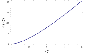
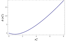
Figure 1: (color online) Plot of the phase shift $\delta(\pi_{+})$ of Eq. (52) for $n_{1}=1$ (left) and for $n_{1}=4$ (right). Changing the value of $n_{1}$ introduces a linear additive term.

III.2 Quantum energy-dependent wall approximation

The reflection coefficient for an infinite wall situated at $\beta_{+}=a$, denoted by $R_{wall}(\pi_{+}^{\infty})$, is given by

$$R_{wall}(\pi_{+}^{\infty})=-e^{2ia\,\pi_{+}^{\infty}}\,.$$ (53)

Therefore, we can interpret the phase shift of Eq. (52) as being the one of a $\pi_{+}^{\infty}$-dependent infinite wall situated at $\beta_{+}=\beta_{+}^{(Q)}$ with

$$\beta_{+}^{(Q)}=\frac{1}{2\pi_{+}^{\infty}}\delta(\pi_{+}^{\infty})=-\frac{i}{2\pi_{+}^{\infty}}\int_{0}^{\pi_{+}^{\infty}}\frac{R^{\prime}(x)}{R(x)}\mathrm{d}x\,.$$ (54)

Now, from $\beta_{+}^{(C)}$ of Eq. (31) obtained at classical level, and $\beta_{+}^{(Q)}$ of Eq. (54) obtained from quantum calculations, we obtain two different possible approximations in terms of infinite walls. We will show in what follows that these approximations give completely different behavior for small values of $\pi_{+}^{\infty}$.

III.3 The behavior of $\delta(\pi_{+}^{\infty})$

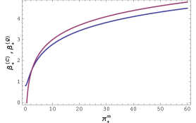
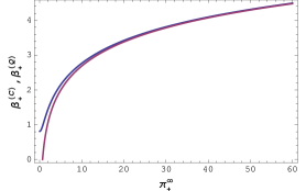
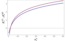
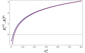
Figure 2: (color online) Plots of $\beta_{+}^{(C)}$ (red curve) and $\beta_{+}^{(Q)}$ (blue curves) for $n_{1}=1$ (top) and for $n_{1}=4$ (bottom). Changing the value of $n_{1}$ introduces the same shift on $\beta_{+}^{(C)}$ and $\beta_{+}^{(Q)}$. The left plots are without any correction; on the right, $\beta_{+}^{(C)}$ has been shifted with $\delta\beta_{\infty}=\ln 2/e$.

III.3.1 The case of large $\pi_{+}^{\infty}$

For large values of $\pi_{+}^{\infty}$ we obtain

$$\beta_{+}^{(Q)}=\ln\frac{4\pi_{+}^{\infty}}{e\,n_{1}}+O(1/\pi_{+}^{\infty})\,.$$ (55)

Therefore the dominant classical and quantum expressions are equivalent

$$\beta_{+}^{(Q)}\sim\ln\pi_{+}^{\infty}\sim\beta_{+}^{(C)}\,.$$ (56)

But there remains a small difference, since $\lim_{\pi_{+}^{\infty}\to\infty}(\beta_{+}^{(Q)}-\beta_{+}^{(C)})=\delta\beta_{\infty}=\ln 2/e$. This is shown in Fig. 2. This shift $\delta\beta_{\infty}$ is a methodological bias that does not contain any physical meaning. Actually we chose some “reasonable” definitions of the locations $\beta_{+}^{(C)}$ and $\beta_{+}^{(Q)}$ of the classical and quantum walls. Therefore, it is not surprising that we find finally some small numerical difference. In the remainder we introduce the modified classical location $\tilde{\beta}_{+}^{(C)}=\beta_{+}^{(C)}+\delta\beta_{\infty}$, corresponding to the nonvanishing asymptotic part of $\beta_{+}^{(Q)}$. We conclude that for large values of $\pi_{+}^{\infty}$, classical and quantum calculations give similar results.

III.3.2 The case of small $\pi_{+}^{\infty}$

Making the power series of $\delta(\pi_{+}^{\infty})$ defined in Eq. (52), near $\pi_{+}^{\infty}=0$, we obtain

$$\delta(\pi_{+}^{\infty})=-2(\gamma+\ln(n_{1}/4))\pi_{+}^{\infty}+O((\pi_{+}^{\infty})^{3})\,,$$ (57)

where $\gamma\simeq 0.5772$ is the Euler-Mascheroni constant. Therefore we obtain from Eq. (54)

$$\beta_{+}^{(Q)}=-(\gamma+\ln(n_{1}/4))+O((\pi_{+}^{\infty})^{2})\,,$$ (58)

while from Eq. (31), $\tilde{\beta}_{+}^{(C)}=\ln(4\pi_{+}^{\infty}/e\,n_{1})$ and then $\tilde{\beta}_{+}^{(C)}\to-\infty$ when $\pi_{+}^{\infty}\to 0$ (see Fig. 3).
Furthermore, we find $\beta_{+}^{(Q)}\simeq-(\gamma+\ln(n_{1}/4))$ up to the second order. Therefore, an infinite wall located at a fixed position $\beta_{+}^{0}=-(\gamma+\ln(n_{1}/4))$ is a very good approximation (at the quantum level), for small values of $\pi_{+}^{\infty}$. This is a pure quantum result that does not possess any classical counterpart. But if we transfer this picture in the classical domain (to obtain a semiclassical description), this means that for small values of $\pi_{+}^{\infty}$, the accessible $\beta_{+}$ domain is defined by $\beta_{+}\leq\beta_{+}^{0}$, which corresponds in the old variable $q_{1}=e^{\beta_{+}}$ to the constraint

$$q_{1}\leq\frac{4\hbar\,\tilde{\kappa}\,e^{-\gamma}}{n_{1}}\,.$$ (59)

To restore the $\hbar_{b}$ dependence, we only have to change $\pi_{+}^{\infty}\to\pi_{+}^{\infty}/\hbar_{b}$ and $n_{1}\to n_{1}/\hbar_{b}$ in the expressions of $R$, $\delta$, and $\beta_{+}^{(Q)}$. Therefore, the classical limit $\hbar_{b}\to 0$ corresponds to the previous analysis $\pi_{+}^{\infty}\to\infty$, and we recover the asymptotic equality between classical and quantum prescriptions. The special value $\beta_{+}^{0}$ reads $\beta_{+}^{0}=-(\gamma+\ln(n_{1}/4\hbar_{b}))$; then, when $\hbar_{b}\to 0$, $\beta_{+}^{0}\to-\infty$ and we recover the classical result $\lim_{\pi_{+}^{\infty}\to 0}\tilde{\beta}_{+}^{(C)}=-\infty$.

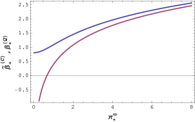
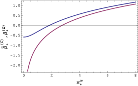
Figure 3: (color online) Plots of $\tilde{\beta}_{+}^{(C)}$ (red curve) and $\beta_{+}^{(Q)}$ (blue curve) for $n_{1}=1$ (left) and for $n_{1}=4$ (right) and small values of $\pi_{+}^{\infty}$.

IV Summary and outlook

We have shown explicitly the asymptotic equivalence of classical Bianchi I and II models: as time goes to $\pm\infty$, the solutions to the dynamics of the two models coincide. This circumstance was used to consider the quantum dynamics of the Bianchi II model in terms of scattering process. However, the interpretation of the Hamiltonian (34) as that of a particle with mass dependent on its position in space is quite formal. The cosmological interpretation is that the Kasner universe approaching the singularity undergoes a rapid external push to its scale factors due to the intrinsic curvature of the Bianchi II model.

The results presented, for small and large values of $\pi_{+}^{\infty}$, exhibit the main common features and differences between classical and quantum formulations. As expected, differences become important when the nonlocality due to quantum mechanics cannot be neglected, i.e. when the uncertainty $\Delta\beta_{+}\sim 1/\pi_{+}^{\infty}$ is very large. The Bianchi II model is important because it bridges the two Kasner universes. We found that the quantization of the Bianchi II dynamics leads to a limited departure from the classical picture.

Roughly speaking, the classical evolution of the Bianchi IX model BKL22 towards the cosmological singularity can be considered to be a sequence of transitions from one Kasner epoch to another one via the vacuum Bianchi II type evolution. This sequence can be divided into eras which differ from one another by oscillations of distances along different pairs of generalized Kasner’s axes BKL22 ; Reiterer:2010cz . We are aware that the classical picture needs not extend to the quantum level. We expect that the quantum dynamics of the Bianchi II model presented in this paper may be used, to some extent, as a building block for quantum evolution of the Bianchi IX model to be examined in the near future. Such procedure would consist in finding the suitable way of sewing together two consecutive quantum Bianchi II models.

One the important question remainsto be answered: How can we deal with the classical singularity of the Bianchi II model at the quantum level? As far as we are aware, this problem has not been addressed satisfactorily yet. Some kernels of the dynamical constraints of the Bianchi class A models have been found, but the Hilbert spaces based on them have not been constructed TCh ; JEL . We plan to address this issue elsewhere.

References

(1) V. A. Belinskii, I. M. Khalatnikov, and E. M. Lifshitz,
Adv. Phys. 19, 525(1970).
(2) V. A. Belinskii, I. M. Khalatnikov, and E. M. Lifshitz, Adv. Phys. 31, 639 (1982).
(3)
M. Reiterer and E. Trubowitz,
arXiv:1005.4908; R. Galimova, arXiv:1403.2767.
(4) C. W. Misner,
Phys. Rev. 186, 1319 (1969).
(5) C. W. Misner, in Magic Without
Magic: John Archibald Wheeler, edited by J. R. Klauder (W.H.
Freeman and Company, San Francisco, 1972), p. 441.
(6) O. I. Bogoyavlensky, Methods in the Qualitative Theory
of Dynamical Systems in Astrophysics and Gas Dynamics
(Springer-Verlag, Berlin, 1985).
(7)
A. Ashtekar and E. Wilson-Ewing,
Phys. Rev. D 79, 083535 (2009).
(8)
A. Ashtekar and E. Wilson-Ewing,
Phys. Rev. D 80, 123532 (2009).
(9)
E. Wilson-Ewing,
Phys. Rev. D 82, 043508 (2010).
(10) M. P. Ryan, Jr., and L. C. Sheply, Homogeneous Relativistic
Cosmologies (Princeton University Press, Princeton, NJ, 1975).
(11)
P. Dzierzak and W. Piechocki,
Phys. Rev. D 80, 124033 (2009).
(12)
P. Malkiewicz, W. Piechocki and P. Dzierzak,
Classical Quantum Gravity 28, 085020 (2011).
(13)
P. Malkiewicz,
Classical Quantum Gravity 29, 075008 (2012).
(14) T. Christodoulakis, G. Kofinas, E. Korfiatis, and A. Paschos,
Phys. Lett. B 390, 55 ( 1997).
(15) J. E. Lidsey,
Phys. Lett. B 352, 207 ( 1995).
(16) M. Henneaux and C. Teitelboim, Quantization of Gauge
Systems (Princeton University Press, Princeton, NJ, 1992).