Distributed bargaining in dyadic-exchange networks

Abstract

This paper considers dyadic-exchange networks in which individual agents autonomously form coalitions of size two and agree on how to split a transferable utility. Valid results for this game include stable (if agents have no unilateral incentive to deviate), balanced (if matched agents obtain similar benefits from collaborating), or Nash (both stable and balanced) outcomes. We design provably-correct continuous-time algorithms to find each of these classes of outcomes in a distributed way. Our algorithmic design to find Nash bargaining solutions builds on the other two algorithms by having the dynamics for finding stable outcomes feeding into the one for finding balanced ones. Our technical approach to establish convergence and robustness combines notions and tools from optimization, graph theory, nonsmooth analysis, and Lyapunov stability theory and provides a useful framework for further extensions. We illustrate our results in a wireless communication scenario where single-antenna devices have the possibility of working as 2-antenna virtual devices to improve channel capacity.

I Introduction

Networked systems, characterized by distributed interactions among multiple components and across several layers, are pervasive in modern engineering problems and also model various biological, economic, and sociological processes. Our motivation in this work is driven by resource-constrained networks where collaboration between subsystems gives rise to a more efficient use of the resources. To this end, we view each subsystem as a player in a coalitional game where neighboring players seek to form a match (i.e., a coalition of size two) and split the corresponding transferable utility between the matched agents. Our aim is to synthesize distributed bargaining mechanisms that agents can employ to decide with whom to collaborate with and how to allocate the utility. Our interest in distributed strategies is motivated by the inherent limitations posed by the network structure, privacy concerns, and scalability and robustness considerations for implementation.

Literature review. Examples of networked systems where performance benefits arise from agents cooperating with each other towards the achievement of a common goal are by now pervasive, see e.g. [1, 2, 3] and references therein. Of particular relevance to this paper are scenarios where individual agents have the ability to carry out their objectives satisfactorily by themselves, but performance can be improved by collaborating with others. Examples are also numerous and include resource allocation in communication networks [4, 5, 6], formation creation in networks of UAVs [7], network security [8], mobile robot coordination [9], large-scale data processing [10], and applications in sociology [11] and economics [12]. Bargaining problems of the type considered here are posed on dyadic-exchange networks, so called because agents can match with at most one other agent [13]. Bipartite matching and assignment problems [14] are special cases of the dyadic-exchange network. Nash bargaining outcomes are an extension to multi-player games of the classical two-player Nash bargaining solution [15]. The works [16, 17] develop centralized methods for finding such outcomes. In terms of distributed implementations, the work [18] provides a discrete-time dynamics that, given a matching, converges to balanced allocations and [19] provides a discrete-time dynamics that converges to Nash outcomes (without considering dynamics separately for stable or balanced outcomes). With respect to these works, an important novelty of the present manuscript is the dynamics and control perspective on this class of problems, which allows us to develop a principled technical approach to the study of asymptotic convergence and robustness. Another area of connection with the literature is the body of research on distributed algorithms for solving linear programs [20, 21], including the authors’ previous work [22]. Our algorithmic design to find stable outcomes builds on the distributed algorithm proposed in [22] because of its mild requirements for guaranteeing convergence and its robustness properties against disturbances.

Statement of contributions. We consider dyadic-exchange networks where individual agents bargain with one another about whom to match with and how to allocate the transferable utility associated to a matching. For this scenario, the type of outcomes we are interested in are Nash bargaining solutions, which combine the notion of stability and fairness. A stable outcome is one where none of the agents benefit by unilaterally deviating from their match. A balanced outcome is one where matched agents benefit equally from the match, where benefit is defined as the next-best allocation that an agent could achieve by a unilateral deviation. The main contribution of the paper is the design of provably-correct distributed continuous-time dynamics that find each of these classes of outcomes. The problem of finding stable outcomes is combinatorial in the number of edges in the network. Nevertheless, we build on the correspondence between the existence of stable outcomes and the solutions of a linear programming relaxation for the maximum weight matching problem on the graph to synthesize a distributed algorithm that determines stable outcomes. Regarding balanced outcomes, we note how finding them requires each pair of matched agents to solve a system of coupled nonlinear equations. Based on this observation, we define local (with respect to $2$-hop information) error functions that measure how far matched agents’ allocations are from being balanced. Our proposed distributed algorithm has then agents adjust their allocations based on their balancing errors. Finally, we interconnect the two aforementioned dynamics to synthesize a distributed algorithm that finds Nash bargaining solutions. We show how the ‘stable outcome’ part of the dynamics allows agents to guess in a distributed way with whom to match and that this prediction becomes correct in finite time. Based on this prediction, the ‘balanced outcome’ part of the dynamics asymptotically converges to a Nash outcome. As a byproduct of the systems and control perspective adopted here, we also assess the robustness properties of the proposed distributed algorithm against small perturbations. Our technical approach combines notions and tools from distributed linear programming, graph theory, nonsmooth analysis, and Lyapunov stability techniques. We conclude by applying our results to a wireless communication scenario in which multiple devices send data to a base station according to a time division multiple access protocol. Devices may share their transmission time slots in order to gain an improved channel capacity. Simulation results show how agents find a Nash outcome in a distributed way, yielding fair capacity improvements for each matched device and a network-wide capacity improvement of around $16\%$.

Organization. Section II introduces notation and background material used throughout the paper. Section III introduces the problem of designing distributed algorithms to find stable, balanced, and Nash outcomes. Sections IV, V, and VI provide, respectively, our algorithmic solutions for each of these classes of outcomes. Section VII presents simulations results and finally Section VIII gathers our conclusions and ideas for future work.

II Preliminaries

This section introduces basic preliminaries on notation, nonsmooth analysis, set-valued dynamical systems, and distributed linear programming.

II-A Notation

We denote the set of real and nonnegative real numbers by $\mathbb{R}$ and $\mathbb{R}_{\geq 0}$, respectively. For a set $X\subseteq\mathbb{R}^{n}$, its intersection with the nonnegative orthant is denoted $X_{+}:=X\cap\mathbb{R}_{\geq 0}^{n}$. This notation is applied analogously to vectors and scalars. For $x\in\mathbb{R}^{n}$, we use $x\geq 0$ (resp. $x>0$) to mean that all components of $x$ are nonnegative (resp. positive). We let $\bar{S}$ denote the closure of the set $S$. Given sets $S_{1}$ and $S_{2}$, $S_{1}\setminus S_{2}$ denotes the complement of $S_{2}$ in $S_{1}$. A set $S\subseteq{}^{n}$ is convex if it fully contains the segment connecting any two points in $S$. The set $\mathbb{B}(x,\delta)\subseteq\mathbb{R}^{n}$ is the open ball centered at $x\in\mathbb{R}^{n}$ with radius $\delta>0$. We use the shorthand notation $S+\mathbb{B}(0,\delta)$ to denote the union $\cup_{x\in S}\mathbb{B}(x,\delta)$. Given a matrix $A\in{}^{n\times m}$, we let $A_{i}$ denote the $i^{\operatorname{th}}$ row of $A$ and $a_{i,j}$ its $(i,j)$ element.

II-B Nonsmooth analysis

Here we review some basic notions from nonsmooth analysis following [23]. A function $f:\mathbb{R}^{n}\rightarrow\mathbb{R}$ is locally Lipschitz at $x\in\mathbb{R}^{n}$ if there exist $\delta_{x}>0$ and $L_{x}\geq 0$ such that $\|f(y_{1})-f(y_{2})\|\leq L_{x}\|y_{1}-y_{2}\|$ for $y_{1},y_{2}\in\mathbb{B}(x,\delta_{x})$. We refer to $f$ simply as locally Lipschitz if $f$ is locally Lipschitz at all $x\in\mathbb{R}^{n}$. A locally Lipschitz function is differentiable almost everywhere. Letting $\Omega_{f}\subseteq\mathbb{R}^{n}$ be the set of points where the locally Lipschitz function $f$ is not differentiable, the generalized gradient of $f$ at $x\in\mathbb{R}^{n}$ is

$$\partial f(x)=\operatorname{co}\Big{\{}\lim_{i\rightarrow\infty}\nabla f(x_{i}):x_{i}\rightarrow x,x_{i}\notin S\cup\Omega_{f}\Big{\}},$$

where $\operatorname{co}\{\cdot\}$ denotes the convex hull and $S\subseteq\mathbb{R}^{n}$ is any set with zero Lebesgue measure. We use $\partial_{x}g(x,y)$ and $\partial_{x}g(x,y)$ to denote the generalized gradient of the maps $x\mapsto g(x,y)$ and $y\mapsto g(x,y)$, respectively.

A set-valued map $F:\mathbb{R}^{n}\rightrightarrows\mathbb{R}^{n}$ maps elements in $\mathbb{R}^{n}$ to subsets of $\mathbb{R}^{n}$. A set-valued map $F$ is locally bounded if for every $x\in\mathbb{R}^{n}$ there exists an $\epsilon>0$ such that $F(\mathbb{B}(x,\epsilon))$ is bounded. A set-valued map $F$ is upper semi-continuous if for all $x\in\mathbb{R}^{n}$ and $\epsilon\geq 0$, there exists $\delta_{x}\geq 0$ such that $F(y)\subseteq F(x)+\mathbb{B}(0,\epsilon)$ for all $y\in\mathbb{B}(x,\delta_{x})$. Given a locally Lipschitz function $f:\mathbb{R}^{n}\rightarrow\mathbb{R}$, the generalized gradient map $x\mapsto\partial f(x)$ is a locally bounded and upper semi-continuous set-valued map. Moreover, $\partial f(x)$ is nonempty, convex, and compact for all $x\in\mathbb{R}^{n}$.

II-C Set-valued dynamical systems

We present here basic notions on set-valued dynamical systems following the exposition of [24]. A time-invariant set-valued dynamical system is represented by the differential inclusion

$$\dot{x}\in F(x),$$ (1)

where $F:X\subseteq\mathbb{R}^{n}\rightrightarrows\mathbb{R}^{n}$ is a set-valued map. If $F$ is locally bounded, upper semi-continuous and takes nonempty, convex, and compact values, then, from any initial condition, there exists an absolutely continuous curve $x:\mathbb{R}_{\geq 0}\rightarrow X$ (called trajectory or solution) satisfying (1) almost everywhere. The set of equilibria of $F$ is $\{x\in X:0\in F(x)\}$. A set $\mathcal{M}$ is weakly positively invariant with respect to $F$ if, for any $x_{0}\in\mathcal{M}$, $\mathcal{M}$ contains at least one maximal solution (that is, one that cannot be extended forward in time) of $\dot{x}\in F(x)$ with initial condition $x_{0}$. The set-valued Lie derivative of a locally Lipschitz function $V:\mathbb{R}^{n}\rightarrow\mathbb{R}$ along $F$ at $x\in\mathbb{R}^{n}$ is defined as

$$\mathcal{L}_{F}V(x)=\{a\in\mathbb{R}:\exists v\in F(x)\text{ s.t. }v^{T}\zeta=a\;\forall\zeta\in\partial V(x)\}.$$

One can show that, if $\mathcal{L}_{F}V(x)\subseteq(-\infty,0]$ for all $x\in\mathbb{R}^{n}$, then $V$ is non-increasing along the trajectories of (1).

The following result helps establish the asymptotic convergence properties of (1).

Theorem II.1

(Set-valued LaSalle Invariance Principle). Assume $V:\mathbb{R}^{n}\rightarrow\mathbb{R}$ is differentiable, the trajectories of (1) are bounded, and $F$ is locally bounded, upper semi-continuous and takes nonempty, convex, and compact values. If $\mathcal{L}_{F}V(x)\subseteq(-\infty,0]$ for all $x\in X$, then any trajectory $t\mapsto x(t)$ of (1) starting in $X$ converges to the largest weakly positively invariant set $\mathcal{M}$ contained in $\overline{\{x\in X:0\in\mathcal{L}_{F}V(x)\}}$.

Set-valued dynamical systems are a helpful tool in understanding the solutions of a differential equation

$$\dot{x}=f(x),$$ (2)

when $f:\mathbb{R}^{n}\rightarrow\mathbb{R}^{n}$ is discontinuous. Formally, let $S_{f}$ denote the set of points where $f$ is discontinuous. Define the Filippov set-valued map $\mathcal{F}[f]:\mathbb{R}^{n}\rightrightarrows\mathbb{R}^{n}$ by

$$\mathcal{F}[f](x):=\overline{\operatorname{co}}\big{\{}\lim_{i\rightarrow\infty}f(x_{i}):x_{i}\rightarrow x,\;x_{i}\notin S_{f}\big{\}},$$ (3)

where $\overline{\operatorname{co}}\{\cdot\}$ denotes the closed convex hull. If $f$ is measurable and locally bounded, then $\mathcal{F}[f]$ is locally bounded, upper semi-continuous and takes nonempty, convex, and compact values. In such case, a solution $t\mapsto x(t)$ of (2) in the Filippov sense is a solution to $\dot{x}\in\mathcal{F}[f](x)$.

II-D Distributed linear programming

Our review here of distributed linear programming follows closely the exposition in [25, 22]. A standard form linear program is given by

$$\min\{c^{T}x:Ax=b,\;x\geq 0\},$$ (4)

where $c\in\mathbb{R}^{n},A^{n\times m}$, and $b\in\mathbb{R}^{m}$. Its dual is

$$\max\{-b^{T}z:A^{T}z\geq c\}.$$ (5)

The point $(x^{*},z^{*})\in\mathbb{R}^{n}\times\mathbb{R}^{m}$ satisfies the KKT conditions for (4) if

$$Ax^{*}=b,\quad x^{*}\geq 0,\quad A^{T}z^{*}\geq c,\;\text{ and }\;(A^{T}z^{*}+c)^{T}x^{*}=0.$$

When (4) has a finite optimal value, $x^{*}$ (resp. $z^{*}$) is a solution to (4) (resp. the dual (5)) if and only if $(x^{*},z^{*})$ satisfies the KKT conditions for (4).

We have proposed in [22] the following continuous-time dynamics to solve the linear program (4),

$$\dot{x}_{i} =\begin{cases}f_{i}(x,z),\hskip 48.36967pt\text{if $x_{i}>0$,}\\ \max\{0,f_{i}(x,z)\},\quad\text{if $x_{i}=0$,}\end{cases}$$ (6a)

$$\dot{z} =Ax-b,$$ (6b)

where the nominal flow function, $f:{}^{n}\times\mathbb{R}^{m}\rightarrow\mathbb{R}^{n}$, is defined by

$$f=-c-A^{T}(Ax-b+z).$$ (7)

The convergence properties of this dynamics are captured in the following result.

Theorem II.2

(Convergence to a solution of a linear program). Let $t\rightarrow(x(t),z(t))$ be a trajectory of (6) starting from an initial point in $\mathbb{R}^{n}_{\geq 0}\times\mathbb{R}^{m}$. Then, if (4) has a finite optimal value, the following limit exists

$$\lim_{t\rightarrow\infty}(x(t),z(t))=(x^{*},z^{*}),$$

where $x^{*}$ (resp. $z^{*}$) is a solution to (4) (resp. the dual of (4)).

In addition to the asymptotic convergence of (7) stated in Theorem II.2, here we mention two additional important properties of this dynamics: it is robust to disturbances (specifically, integral input-to-state stable) and amenable to distributed implementation. We elaborate on the latter next, as it is relevant for the main developments of the paper. Suppose that each component of $x\in\mathbb{R}^{n}$ corresponds to the state of an independent decision maker or agent. In order for agent $i\in\{1,\dots,n\}$ to be able to implement its corresponding dynamics in (6a), it needs access to the following data and states:

1. $c_{i}\in\mathbb{R}$,

2. every $b_{\ell}\in\mathbb{R}$ for which $a_{\ell,i}\not=0$,

3. the non-zero elements of every row of $A$ for which the $i^{\text{th}}$ component, $a_{\ell,i}$, is non-zero,

4. the states of every agent $j\in\{1,\dots,n\}$ where $a_{\ell,i}\not=0$ and $a_{\ell,j}\not=0$ for some $\ell\in\{1,\dots,m\}$, and

5. every $z_{\ell}$ for which $a_{\ell,i}\not=0$.

The agents $j$ for which $a_{\ell,i}\not=0$ and $a_{\ell,j}\not=0$ for some $\ell\in\{1,\dots,m\}$ (as in (iv) above) are called neighbors of $i$, denoted $\mathcal{N}(i)$. Also, the states $z_{\ell}$ are auxiliary states whose dynamics can, based on locally available data and states, be implemented by any agent $i$ for which $a_{\ell,i}\not=0$.

III Problem statement

The main objective of the paper is the design of provably correct distributed dynamics that solve the network bargaining game. This section provides a formal description of the problem. We begin by presenting the model for the group of agents and then recall various important notions of outcome for the network bargaining game.

Let $\mathcal{G}=(\mathcal{V},\mathcal{E},W)$ be an undirected weighted graph where $\mathcal{V}=\{1,\dots,n\}$ is a set of vertices, $\mathcal{E}\subseteq\mathcal{V}\times\mathcal{V}$ is a set of edges, and $W\in\mathbb{R}_{\geq 0}^{|\mathcal{E}|}$ is a vector of edge weights indexed by edges in $\mathcal{G}$. In an exchange network, vertices correspond to agents (or players) and edges connect agents who have the ability to negotiate with each other. The set of agents that $i$ can negotiate with are its neighbors and is denoted by $\mathcal{N}(i):=\{j:(i,j)\in\mathcal{E}\}$. Edge weights represent a transferable utility that agents may, should they come to an agreement, divide between them. Here, we assume that the network is a dyadic-exchange network, meaning that agents can pair with at most one other agent. Agents are selfish and seek to maximize the amount they receive. However if two agents $i$ and $j$ cannot come to an agreement, they forfeit the entire amount $w_{i,j}$. We consider bargaining outcomes of the following form.

Definition III.1

(Outcomes). A matching $M\subseteq\mathcal{E}$ is a subset of edges without common vertices. An outcome is a pair $(M,\alpha)$, where $M\subseteq\mathcal{E}$ is a matching and $\alpha\in\mathbb{R}^{n}$ is an allocation to each agent such that $\alpha_{i}+\alpha_{j}=w_{i,j}$ if $(i,j)\in M$ and $\alpha_{k}=0$ if agent $k$ is not part of any edge in $M$. $\bullet$

In any given outcome $(M,\alpha)$, an agent may decide to unilaterally deviate by matching with another neighbor. As an example, suppose that $(i,j)\in M$ and agent $k$ is a neighbor of $i$. If $\alpha_{i}+\alpha_{k}<w_{i,k}$, then there is an incentive for $i$ to deviate because it could receive an increased allocation of $\hat{\alpha}_{i}=w_{i,k}-\alpha_{k}>\alpha_{i}$. Such a deviation is unilateral because $k$’s allocation stays constant. Conversely, if $\alpha_{i}+\alpha_{k}\geq w_{i,k}$, then $i$ does not have an incentive to deviate by matching with $k$. This discussion motivates the notion of a stable outcome, in which no agent benefits from a unilateral deviation.

Definition III.2

(Stable outcome). An outcome $(M,\alpha^{s})$ is stable if $\alpha^{s}\geq 0$ and

$$\alpha^{s}_{i}+\alpha^{s}_{j}\geq w_{i,j},\quad\forall(i,j)\in\mathcal{E}. \bullet$$

Given an arbitrary matching $M$, it is not always possible to find allocations $\alpha^{s}$ such that $(M,\alpha^{s})$ is a stable outcome. Thus, finding stable outcomes requires to find an appropriate matching as well, making the problem combinatorial in the number of possible matchings.

Stable outcomes are not necessarily fair between matched agents, and this motivates the notion of balanced outcomes. As an example, again assume that the outcome $(M,\alpha^{b})$ is given and that $(i,j)\in M$. The best allocation that $i$ could expect to receive by matching with a neighbor other than $j$ is

$$\texttt{ba}_{{i}\setminus{j}}(\alpha^{b})=\max_{k\in\mathcal{N}(i)\setminus j}\{w_{i,k}-\alpha^{b}_{k}\}_{+}.$$

Moreover, the set (possibly empty) of best neighbors with whom $i$ could receive this allocation is

$$\texttt{bn}_{{i}\setminus{j}}(\alpha^{b})=\operatorname{argmax}_{k\in\mathcal{N}(i)\setminus j}\{w_{i,k}-\alpha^{b}_{k}\}_{+}.$$

Then, if agent $i$ were to unilaterally deviate from the outcome and match instead with $k\in\texttt{bn}_{{i}\setminus{j}}$, the resulting benefit of this deviation would be

$$\texttt{ba}_{{i}\setminus{j}}(\alpha^{b})-\alpha^{b}_{i}.$$

When the benefit of a deviation is the same for both $i$ and $j$, we call the outcome balanced.

Definition III.3

(Balanced outcome). An outcome $(M,\alpha^{b})$ is balanced if for all $(i,j)\in M$,

$$\texttt{ba}_{{i}\setminus{j}}(\alpha^{b})-\alpha^{b}_{i}=\texttt{ba}_{{j}\setminus{i}}(\alpha^{b})-\alpha^{b}_{j}. \bullet$$

From its definition, it is easy to see that the main challenge in finding balanced outcomes is the fact that the allocations must satisfy a system of nonlinear (in fact, piecewise linear) equations, coupled between agents. Of course, outcomes that are both stable and balanced are desirable and what we seek in this paper. Such outcomes are called Nash.

Definition III.4

(Nash outcome). An outcome $(M,\alpha^{N})$ is Nash if it is stable and balanced. $\bullet$

Figure 1 shows an example of each outcome, highlighting their various attributes.

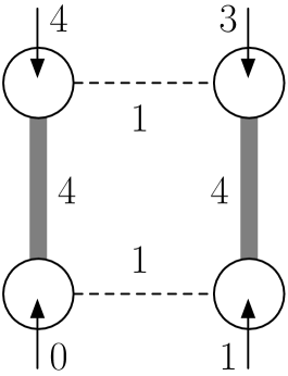
(a) Stable

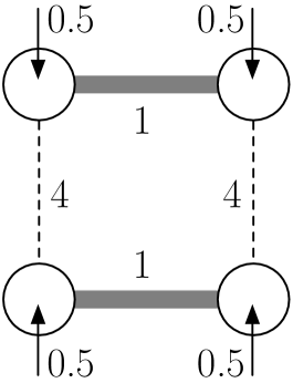
(b) Balanced

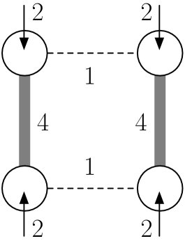
(c) Nash

Figure 1: For each outcome, matched agents are connected with thicker grey edges, dotted edges connect agents who decided not to match, and allocations are indicated by arrows. In the stable outcome, the $0$ allocation is unfair to that node since its partner receives the whole edge weight. In the balanced outcome, agents can receive higher allocations by deviating from their matches. Nash outcomes do not exhibit either of these shortcomings.

The problem we aim to solve is to develop distributed dynamics that converge to each of the class of outcomes defined above: stable, balanced, and Nash. We refer to a dynamics as $1$-hop distributed, or simply distributed, over $\mathcal{G}$ if its implementation requires each agent $i\in\{1,\dots,n\}$ only knowing (i) the states of $1$-hop neighboring agents and (ii) the utilities $w_{i,j}$ for each $j\in\mathcal{N}(i)$. Likewise, we refer to a dynamics as $2$-hop distributed over $\mathcal{G}$ if its implementation requires each agent $i\in\{1,\dots,n\}$ only knowing (i) the states of $1$- and $2$-hop neighboring agents and (ii) the utilities $w_{i,j}$ and $w_{j,k}$ for each $j\in\mathcal{N}(i)$ and $k\in\mathcal{N}(j)$. As agents’ allocations evolve in the dynamics that follow, the quantity $w_{i,j}-\alpha_{i}(t)$ has the interpretation of “$i$’s offer to $j$ at time $t$”, thus motivating the terminology bargaining in exchange networks.

IV Distributed dynamics to find stable outcomes

In this section, we propose a distributed dynamics to find stable outcomes in network bargaining. Our strategy to achieve this builds on a reformulation of the problem of finding a stable outcome in terms of finding the solutions to a linear program.

IV-A Stable outcomes as solutions of linear program

Here we relate the existence of stable outcomes to the solutions of a linear programming relaxation for the maximum weight matching problem. This reformulation allows us later to synthesize a distributed dynamics to find stable outcomes. Our discussion here follows [16], but because that reference does not present formal proofs of the results we need, we include them here for completeness.

We begin by recalling the formulation of the maximum weight matching problem on $\mathcal{G}$. Essentially, this corresponds to a matching in which the sum of the edge weights in the matching is maximal. Formally, for every $(i,j)\in\mathcal{E}$ we use variables $m_{i,j}\in\{0,1\}$ to indicate whether $(i,j)$ is in the maximum weight matching (i.e., $m_{i,j}=1$) or not ($m_{i,j}=0$). Then, the solutions of the following integer program can be used to deduce a maximum weight matching,

$$\max \quad\text{\footnotesize$\sum$}_{(i,j)\in\mathcal{E}}w_{i,j}m_{i,j}$$ (8a)

s.t. $$\quad\text{\footnotesize$\sum$}_{j\in\mathcal{N}(i)}m_{i,j}\leq 1,\quad\forall i\in\mathcal{V},$$ (8b)

$$\quad m_{i,j}\in\{0,1\},\quad\forall(i,j)\in\mathcal{E}.$$ (8c)

The constraints (8b) ensure that each agent is matched to at most one other agent. If $m^{*}\in\{0,1\}^{|\mathcal{E}|}$ is a solution (indexed by edges in $\mathcal{G}$) to the above optimization problem, then a maximum weight matching is well-defined by the relationship $(i,j)\in M\Leftrightarrow m^{*}_{i,j}=1$. Since (8) is combinatorial in the number of edges in the graph due to constraint (8c), we are interested in studying its linear programming relaxation,

$$\max \quad\text{\footnotesize$\sum$}_{(i,j)\in\mathcal{E}}w_{i,j}m_{i,j}$$

s.t. $$\quad\text{\footnotesize$\sum$}_{j\in\mathcal{N}(i)}m_{i,j}\leq 1,\quad\forall i\in\mathcal{V},$$ (9)

$$\quad m_{i,j}\geq 0,\quad\forall(i,j)\in\mathcal{E},$$

and its associated dual

$$\min \quad\text{\footnotesize$\sum$}_{i\in\mathcal{V}}\alpha^{s}_{i}$$

s.t. $$\quad\alpha^{s}_{i}+\alpha^{s}_{j}\geq w_{i,j},\quad\forall(i,j)\in\mathcal{E},$$ (10)

$$\quad\alpha^{s}_{i}\geq 0,\quad\forall i\in\mathcal{V}.$$

Arguing with the KKT conditions for the relaxation (IV-A), the following result states that when a stable outcome $(M,\alpha^{s})$ exists, the matching $M$ is a maximum weight matching on $\mathcal{G}$.

Lemma IV.1

(Maximum weight matchings and stable outcomes [16]). Suppose that a stable outcome $(M,\alpha^{s})$ exists for a given graph $\mathcal{G}$. Then $M$ is a maximum weight matching.

Proof.

Our proof method is to encode the matching $M$ using the indicator variables $m\in\{0,1\}^{|\mathcal{E}|}$ and then show that $m$ is a solution of the maximum weight matching problem (8). To begin, for all $(i,j)\in\mathcal{E}$, let $m_{i,j}=1$ if $(i,j)\in M$ and zero otherwise. Use $m$ to denote the vector of $m_{i,j}$, indexed by edges in $\mathcal{G}$. Then $m$ is feasible for the relaxation (IV-A). By definition of outcome, cf. Definition III.1, it holds that $m_{i,j}(\alpha^{s}_{i}+\alpha^{s}_{j}-w_{i,j})=0$ for all $(i,j)\in\mathcal{E}$ and $\alpha^{s}_{i}(1-\sum_{j\in\mathcal{N}(i)}m_{i,j})=0$ for all $i\in\mathcal{V}$. In other words, complementary slackness is satisfied. Also, note that $\alpha^{s}$ is feasible for the dual (IV-A). This means that $(m,\alpha^{s})$ satisfy the KKT conditions for (IV-A) and so $m$ is a solution of (IV-A). Since $m$ is integral, it is also a solution of (8) implying that $M$ is a maximum weight matching. This completes the proof. ∎

Building on this result, we show next that the existence of stable outcomes is directly related to the existence of integral solutions of the linear programming relaxation (IV-A).

Lemma IV.2

(Existence of stable outcomes [16]). A stable outcome exists for the graph $\mathcal{G}$ if and only if (IV-A) admits an integral solution. Moreover, if $\mathcal{G}$ admits a stable outcome and $m^{*}\in\{0,1\}^{|\mathcal{E}|}$ is a solution to (IV-A), then $(M,\alpha^{s,*})$ is a stable outcome where the matching $M$ is well-defined by the implication

$$(i,j)\in M\Leftrightarrow m^{*}_{i,j}=1,$$ (11)

and $\alpha^{s,*}$ is a solution to (IV-A).

Proof.

The proof of Lemma IV.1 revealed that, if a stable outcome exists, (IV-A) admits an integral solution. Let us prove the other direction. By assumption, (IV-A) yields an integral solution $m^{*}\in\{0,1\}^{|\mathcal{E}|}$ and let $\alpha^{s,*}$ be a solution to the dual (IV-A). We induce the following matching: $(i,j)\in M$ if $m^{*}_{i,j}=1$ and $(i,j)\notin M$ otherwise. By complementary slackness, $m^{*}_{i,j}(\alpha^{s,*}_{i}+\alpha^{s,*}_{j}-w_{i,j})=0$ for all $(i,j)\in\mathcal{E}$ and $\alpha^{s,*}_{i}(1-\sum_{j\in\mathcal{N}(i)}m^{*}_{i,j})=0$ for all $i\in\mathcal{V}$. Then, it must be that $m^{*}_{i,j}=1$ implies that $\alpha^{s,*}_{i}+\alpha^{s,*}_{j}=w_{i,j}$ and $\alpha^{s,*}_{i}=0$ if $i$ is not part of any matching. Thus, $(M,\alpha^{s,*})$ is a valid outcome. Next, $\alpha^{s,*}$ must be feasible for (IV-A), which reveals that it is a stable allocation. Therefore, $(M,\alpha^{s,*})$ is a stable outcome. This completes the proof. ∎

IV-B Stable outcomes via distributed linear programming

Since we are interested in finding stable outcomes, from here on we make the standing assumption that one exists and that the maximum weight matching is unique. Besides its technical implications, requiring uniqueness has a practical motivation and is a standard assumption in exchange network bargaining. For example, if an agent has two equally good alternatives, it is unclear with whom it will choose to match with. It turns out that the set of graphs for which a unique maximum weight matching exists is open and dense in the set of graphs that admit a stable outcome, further justifying the assumption of uniqueness of the maximum weight matching.

Given the result in Lemma IV.2 above, finding a stable outcome is a matter of solving the relaxed maximum weight matching problem, where the matching is induced from the solution of (IV-A) and the allocation is a solution to (IV-A). Our next step is to put (IV-A) in standard form by introducing slack variables $s_{i,j}$ for each $(i,j)\in\mathcal{E}$,

$$\min \quad\text{\footnotesize$\sum$}_{i\in\mathcal{V}}\alpha^{s}_{i}$$

s.t. $$\quad\alpha^{s}_{i}+\alpha^{s}_{j}-s_{i,j}=w_{i,j},\quad\forall(i,j)\in\mathcal{E},$$

$$\quad\alpha^{s}_{i}\geq 0\quad\forall i\in\mathcal{V},$$

$$\quad s_{i,j}\geq 0\quad\forall(i,j)\in\mathcal{E}.$$

We use the notation $s$ to represent the vector of slacks indexed by edges in $\mathcal{G}$. In the dynamics that follow, the variables $s$ and $m$ will be states. Thus, as a convention, we assume that each $s_{i,j}$ and $m_{i,j}$ are states of agent $\min\{i,j\}$. This means that the state of agent $i\in\mathcal{V}$ is

$$(\alpha^{s}_{i},\{s_{i,j}\}_{j\in\mathcal{N}^{+}(i)},\{m_{i,j} \}_{j\in\mathcal{N}^{+}(i)})$$

$$\in\mathbb{R}_{\geq 0}\times\mathbb{R}_{\geq 0}^{|\mathcal{N}^{+}(i)|}\times\mathbb{R}^{|\mathcal{N}^{+}(i)|},$$

where, for convenience, we denote by $\mathcal{N}^{+}(i):=\{j\in\mathcal{N}(i):i<j\}$ the set of neighbors of $i$ whose identity is greater than $i$.

Next, using the dynamics (6) of Section II-D to solve the linear program above results in the following dynamics for agent $i\in\{1,\dots,n\}$,

$$\dot{\alpha}^{s}_{i}=\left\{\begin{aligned} &f^{\alpha}_{i}(\alpha^{s},s,m),&&\quad\alpha^{s}_{i}>0,\\ &\max\{0,f^{\alpha}_{i}(\alpha^{s},s,m)\},&&\quad\alpha^{s}_{i}=0,\end{aligned}\right.$$ (13a)

and, for each $$j\in\mathcal{N}^{+}(i)$$

$$\dot{s}_{i,j} =\left\{\begin{aligned} &f^{s}_{i,j}(\alpha^{s},s,m),&&\quad s_{i,j}>0,\\ &\max\{0,f^{s}_{i,j}(\alpha^{s},s,m)\},&&\quad s_{i,j}=0,\end{aligned}\right.$$ (13b)

$$\dot{m}_{i,j} =\alpha^{s}_{i}+\alpha^{s}_{j}-s_{i,j}-w_{i,j},$$ (13c)

where

$$f^{\alpha}_{i}(\alpha^{s},s,m):=-1\!-\!\sum_{j\in\mathcal{N}(i)}\bigg{[}m_{i,j}+\alpha^{s}_{i}+\alpha^{s}_{j}-s_{i,j}-w_{i,j}\bigg{]},$$

and

$$f^{s}_{i,j}(\alpha^{s},s,m):=-m_{i,j}-\alpha^{s}_{i}-\alpha^{s}_{j}+s_{i,j}+w_{i,j},$$

are derived from (7). The next result reveals how this dynamics can be used as a distributed algorithm to find stable outcomes.

Proposition IV.3

(Convergence to stable outcomes). Given a graph $\mathcal{G}$, let $t\rightarrow(\alpha^{s}(t),s(t),m(t))$ be a trajectory of (13) starting from an initial point in $\mathbb{R}^{n}_{\geq 0}\times\mathbb{R}_{\geq 0}^{|\mathcal{E}|}\times\mathbb{R}^{|\mathcal{E}|}$. Then the following limit exists

$$\lim_{t\rightarrow\infty}(\alpha^{s}(t),s(t),m(t))=(\alpha^{*},s^{*},m^{*}),$$

where $(\alpha^{s,*},s^{*})$ (resp. $m^{*}$) is a solution to (IV-A) (resp. (IV-A)). Moreover, if a stable outcome exists, a maximum weight matching $M$ is well-defined by the implication

$$(i,j)\in M\quad\Leftrightarrow\quad m^{*}_{i,j}=1,$$

and $(M,\alpha^{s,*})$ is a stable outcome. Finally, the dynamics (13) is distributed over $\mathcal{G}$.

The proof of the above results follows directly from Theorem II.2, Lemma IV.2, and the assumptions made on the information available to each agent.

V Distributed dynamics to find balanced outcomes

In this section, we introduce distributed dynamics that converge to balanced outcomes. Our starting point is the availability of a matching $M$ to the network, i.e., each agent already knows if it is matched and who its partner is. Hence, the dynamics focuses on negotiating the allocations to find a balanced one. We drop this assumption later when considering Nash outcomes.

Our algorithm design is based on the observation that the condition $\alpha^{b}_{i}+\alpha^{b}_{j}=w_{i,j}$ for $(i,j)\in M$ that defines an allowable allocation for an outcome and the balance condition in Definition III.3 for two matched agents can be equivalently stated as

$$0\! =\!\alpha^{b}_{i}\!-\!\frac{1}{2}(w_{i,j}\!+\texttt{ba}_{{i}\setminus{j}}(\alpha^{b})\!-\texttt{ba}_{{j}\setminus{i}}(\alpha^{b}))=:e^{b}_{i}(\alpha^{b}),$$ (14a)

$$0\! =\!\alpha^{b}_{j}\!-\!\frac{1}{2}(w_{i,j}\!-\texttt{ba}_{{i}\setminus{j}}(\alpha^{b})\!+\texttt{ba}_{{j}\setminus{i}}(\alpha^{b}))=:e^{b}_{j}(\alpha^{b}).$$ (14b)

We refer to $e^{b}_{i},e^{b}_{j}:\mathbb{R}^{n}\rightarrow\mathbb{R}$ as the errors with respect to satisfying the balance condition of $i$ and $j$, respectively. For an unmatched agent $k$, we define $e^{b}_{k}=\alpha^{b}_{k}$. We refer to $e^{b}(\alpha^{b})\in\mathbb{R}^{n}$ as the vector of balancing errors for a given allocation. Based on the observation above, we propose the following distributed dynamics whereby agents adjust their allocations proportionally to their balancing errors,

$$\dot{\alpha}^{b} =-e^{b}(\alpha^{b}).$$ (15)

An important fact to note is that the equilibria of the above dynamics are, by construction, allocations in a balanced outcome. Also, note that (15) is continuous and requires agents to know $2$-hop information, because for its pair of matched agents $(i,j)\in M$, agent $i$ updates its own allocation (and hence its offer to $j$) based on $\texttt{ba}_{{j}\setminus{i}}$.

The following result establishes the boundedness of the balancing errors under (15) and is useful later in establishing the asymptotic convergence of this dynamics to an allocation in a balanced outcome with matching $M$.

$$\mathcal{L}_{\mathcal{F}[F]}V(\xi)=\{a\in\mathbb{R}:\text{there exists }v\in\mathcal{F}[F](\xi,\omega)\text{ s.t. }a=\zeta^{T}v\text{ for all }\zeta\in\partial V(\xi)\}$$

$$\;=\bigg{\{}a\in\mathbb{R}:\text{for each }i\in\mathcal{V}\text{ there exists }\lambda^{i}\in\mathbb{R}^{n}_{\geq 0}\text{ with }\sum_{\tau\in\texttt{bn}_{{i}\setminus{j}}(\omega)}\lambda^{i}_{\tau}=1\text{ if }\texttt{bn}_{{i}\setminus{j}}(\omega)\not=\emptyset\text{ and }\mu^{i}\in\mathbb{R}^{n}_{\geq 0}\text{ with }\sum_{\kappa\in\texttt{bn}_{{j}\setminus{i}}(\omega)}\mu^{i}_{\kappa}=1\text{ if }$$

$$\hskip 22.76219pt\texttt{bn}_{{j}\setminus{i}}(\omega)\not=\emptyset\text{ s.t. }a\!=\!\bigg{(}\sum_{i\in\mathcal{V}}h_{i}\bigg{[}\!-\!\xi_{i}-\tfrac{1}{2}\sum_{\tau\in\texttt{bn}_{{i}\setminus{j}}(\omega)}\lambda^{i}_{\tau}\xi_{\tau}+\tfrac{1}{2}\sum_{\kappa\in\texttt{bn}_{{j}\setminus{i}}(\omega)}\mu^{i}_{\kappa}\xi_{\kappa}\bigg{]}\bigg{)}^{T}\!\!\bigg{(}\sum_{i\in\mathbbm{M}(\xi)}\eta_{i}h_{i}\xi_{i}\bigg{)}\text{ for all }\eta\in\mathbb{R}^{n}_{\geq 0}\text{ with}\sum_{i\in\mathbbm{M}(\xi)}\eta_{i}=1\bigg{\}}$$

$$\;=\bigg{\{}a\in\mathbb{R}:\text{for each }i\in\mathbbm{M}(\xi)\text{ there exists }\lambda^{i}\in\mathbb{R}^{n}_{\geq 0}\text{ with }\sum_{\tau\in\texttt{bn}_{{i}\setminus{j}}(\omega)}\lambda^{i}_{\tau}=1\text{ if }\texttt{bn}_{{i}\setminus{j}}(\omega)\not=\emptyset\text{ and }\mu^{i}\in\mathbb{R}^{n}_{\geq 0}\text{ with }\sum_{\kappa\in\texttt{bn}_{{j}\setminus{i}}(\omega)}\mu^{i}_{\kappa}=1\text{ if }$$

$$\hskip 22.76219pt\texttt{bn}_{{j}\setminus{i}}(\omega)\not=\emptyset\text{ s.t. }a=\sum_{i\in\mathbbm{M}(\xi)}\eta_{i}\bigg{(}-\xi_{i}^{2}-\tfrac{1}{2}\sum_{\tau\in\texttt{bn}_{{i}\setminus{j}}(\omega)}\lambda^{i}_{\tau}\xi_{i}\xi_{\tau}+\tfrac{1}{2}\sum_{\kappa\in\texttt{bn}_{{j}\setminus{i}}(\omega)}\mu^{i}_{\kappa}\xi_{i}\xi_{\kappa}\bigg{)}\text{ for all }\eta\in\mathbb{R}^{n}_{\geq 0}\text{ with}\sum_{i\in\mathbbm{M}(\xi)}\eta_{i}=1\bigg{\}}.$$ (17)

Proposition V.1

(Balancing errors are bounded). Given a matching $M$, let $t\mapsto\alpha^{b}(t)$ be a trajectory of (15) starting from any point in $\mathbb{R}^{n}$. Then

$$t\mapsto V(e^{b}(\alpha^{b}(t))):=\tfrac{1}{2}\max_{i\in\mathcal{V}}(e^{b}_{i}(\alpha^{b}(t)))^{2}$$

is non-increasing. Thus, $t\mapsto e^{b}(\alpha^{b}(t))$ lies in a bounded set.

Proof.

Our proof strategy is to compute, for each $i\in\mathcal{V}$, the Lie derivative of $e^{b}_{i}$ along the trajectories of (15). Based on these Lie derivatives, we introduce a new dynamics whose trajectories contain $t\mapsto e^{b}(\alpha^{b}(t))$ and establish the result reasoning with it.

Since $e^{b}_{i}$ is locally Lipschitz, it is differentiable almost everywhere. Let $\Omega_{i}\subseteq\mathbb{R}^{n}$ be the set, of measure zero, of allocations for which $e^{b}_{i}$ is not differentiable. If $i$ is matched, say $(i,j)\in M$, then $\Omega_{i}$ is precisely the set of allocations where at least one of the next best neighbor sets $\texttt{bn}_{{i}\setminus{j}}(\alpha^{b})$ or $\texttt{bn}_{{j}\setminus{i}}(\alpha^{b})$ have more than one element. If $i$ is unmatched, then $\Omega_{i}=\emptyset$. Then, whenever $\alpha^{b}\in\mathbb{R}^{n}\setminus\Omega_{i}$, it is easy to see that for every $i\in\mathcal{V}$,

$$\mathcal{L}_{-e^{b}}e^{b}_{i}(\alpha^{b})=\begin{cases}-e^{b}_{i}(\alpha^{b}),&\text{if $i$ is unmatched or }\\ &\text{if }\texttt{bn}_{{i}\setminus{j}}(\alpha^{b})=\emptyset\\ &\text{and }\texttt{bn}_{{j}\setminus{i}}(\alpha^{b})=\emptyset\\ -e^{b}_{i}(\alpha^{b})+\tfrac{1}{2}e^{b}_{\tau}(\alpha^{b}),&\text{if }\texttt{bn}_{{i}\setminus{j}}(\alpha^{b})=\tau\\ &\text{and }\texttt{bn}_{{j}\setminus{i}}(\alpha^{b})=\emptyset\\ -e^{b}_{i}(\alpha^{b})-\tfrac{1}{2}e^{b}_{\kappa}(\alpha^{b}),&\text{if }\texttt{bn}_{{i}\setminus{j}}(\alpha^{b})=\emptyset\\ &\text{and }\texttt{bn}_{{j}\setminus{i}}(\alpha^{b})=\kappa\\ -e^{b}_{i}(\alpha^{b})+\tfrac{1}{2}e^{b}_{\tau}(\alpha^{b})&-\;\tfrac{1}{2}e^{b}_{\kappa}(\alpha^{b}),\\ &\text{if }\texttt{bn}_{{i}\setminus{j}}(\alpha^{b})=\tau\\ &\text{and }\texttt{bn}_{{j}\setminus{i}}(\alpha^{b})=\kappa.\end{cases}$$

This observation motivates our study of the dynamics

$$\dot{\xi}_{i}=\begin{cases}-\xi_{i},&\text{if $i$ is unmatched or }\\ &\text{if }\texttt{bn}_{{i}\setminus{j}}(\omega)=\emptyset\\ &\text{and }\texttt{bn}_{{j}\setminus{i}}(\omega)=\emptyset\\ -\xi_{i}+\tfrac{1}{2}\xi_{\tau},&\text{if }\texttt{bn}_{{i}\setminus{j}}(\omega)=\tau\\ &\text{and }\texttt{bn}_{{j}\setminus{i}}(\omega)=\emptyset\\ -\xi_{i}-\tfrac{1}{2}\xi_{\kappa},&\text{if }\texttt{bn}_{{i}\setminus{j}}(\omega)=\emptyset\\ &\text{and }\texttt{bn}_{{j}\setminus{i}}(\omega)=\kappa\\ -\xi_{i}+\tfrac{1}{2}\xi_{\tau}-\tfrac{1}{2}\xi_{\kappa},&\text{if }\texttt{bn}_{{i}\setminus{j}}(\omega)=\tau\\ &\text{and }\texttt{bn}_{{j}\setminus{i}}(\omega)=\kappa.\end{cases}$$ (16a)

$$\dot{\omega}_{i}=-\xi_{i}$$ (16b)

for every $i\in\mathcal{V}$, defined on $\mathbb{R}^{n}\times(\mathbb{R}^{n}\setminus\Omega)$, where $\Omega:=\cup_{i\in\mathcal{V}}\Omega_{i}$. For convenience, we use the shorthand notation $F=(F^{1},F^{2}):\mathbb{R}^{n}\times(\mathbb{R}^{n}\setminus\Omega)\rightarrow\mathbb{R}^{n}\times\mathbb{R}^{n}$ to refer to (16). Note that $F$ is piecewise continuous (because $F^{1}$ is piecewise continuous, while $F^{2}$ is continuous). Therefore, we understand its trajectories in the sense of Filippov. Using (3), we compute the Filippov set-valued map, defined on $\mathbb{R}^{n}\times\mathbb{R}^{n}$, for any matched $i$ and $(\xi,\omega)\in\mathbb{R}^{n}\times\mathbb{R}^{n}$, as

$$\mathcal{F}[F^{1}_{i}]( \xi,\omega)=\Big{\{}-\xi_{i}-\tfrac{1}{2}\sum_{\tau\in\texttt{bn}_{{i}\setminus{j}}(\omega)}\lambda^{i}_{\tau}\xi_{\tau}+\tfrac{1}{2}\sum_{\kappa\in\texttt{bn}_{{j}\setminus{i}}(\omega)}\mu^{i}_{\kappa}\xi_{\kappa}:$$

$$\quad\lambda^{i}\in\mathbb{R}^{n}_{\geq 0}\text{ is s.t. }\sum_{\tau\in\texttt{bn}_{{i}\setminus{j}}(\omega)}\lambda^{i}_{\tau}=1\text{ if }\texttt{bn}_{{i}\setminus{j}}(\omega)\not=\emptyset$$

$$\quad\text{and }\mu^{i}\in\mathbb{R}^{n}_{\geq 0}\text{ is s.t. }\sum_{\kappa\in\texttt{bn}_{{j}\setminus{i}}(\omega)}\mu^{i}_{\kappa}=1\text{ if }\texttt{bn}_{{j}\setminus{i}}(\omega)\not=\emptyset\Big{\}}.$$

Here, we make the convention that the empty sum is zero. If $i$ is unmatched, then $\mathcal{F}[F^{1}_{i}](\xi,\omega)=\{-\xi_{i}\}$. Furthermore, $\mathcal{F}[F^{2}_{i}]=\{-\xi_{i}\}$ for all $i\in\mathcal{V}$. Based on the discussion so far, we know that $t\mapsto(e^{b}(\alpha^{b}(t)),\alpha^{b}(t))$ is a Filippov trajectory of (16) with initial condition $(e^{b}(\alpha^{b}(0)),\alpha^{b}(0))\in\mathbb{R}^{n}\times\mathbb{R}^{n}$. Thus, to prove the result, it is sufficient to establish the monotonicity of

$$V(\xi)=\max_{i\in\mathcal{V}}\frac{1}{2}\xi_{i}^{2},$$

along (16). For notational purposes, we denote

$$\mathbbm{M}(\xi):=\operatorname{argmax}_{i\in\mathcal{V}}\frac{1}{2}\xi_{i}^{2}.$$

The generalized gradient of $V$ is

$$\partial V(\xi)=\Big{\{}\sum_{i\in\mathbbm{M}(\xi)}\eta_{i}h_{i}\xi_{i}:\eta\in\mathbb{R}^{n}_{\geq 0}\text{ s.t. }\sum_{i\in\mathbbm{M}(\xi)}\eta_{i}=1\Big{\}},$$

where $h_{i}\in\mathbb{R}^{n}$ is the unit vector with $1$ in its $i^{\operatorname{th}}$ component and $0$ elsewhere. Then, the set-valued Lie derivative of $V$ along $\mathcal{F}[F]$ is given in (V). To upper bound the element in $\mathcal{L}_{\mathcal{F}[F]}V(\xi)$, note that

$$-\tfrac{1}{2}\sum_{\tau\in\texttt{bn}_{{i}\setminus{j}}(\omega)}\lambda^{i}_{\tau}\xi_{i}\xi_{\tau}\leq\tfrac{1}{4}\sum_{\tau\in\texttt{bn}_{{i}\setminus{j}}(\omega)}\lambda^{i}_{\tau}(\xi_{i}^{2}+\xi_{\tau}^{2}),$$

where we have used the inequality $ab\leq\tfrac{1}{2}a^{2}+\tfrac{1}{2}b^{2}$ for $a,b\in\mathbb{R}$. For $\sum_{\tau\in\texttt{bn}_{{i}\setminus{j}}(\omega)}\lambda^{i}_{\tau}=1$ and $i\in\mathbbm{M}(\xi)$ (that is $\xi_{i}^{2}\geq\xi_{\tau}^{2}$ for all $\tau\in\texttt{bn}_{{i}\setminus{j}}(\omega)$), we can further refine the bound as,

$$\tfrac{1}{2}\sum_{\tau\in\texttt{bn}_{{i}\setminus{j}}(\omega)}\lambda^{i}_{\tau}\xi_{i}\xi_{\tau}\leq\tfrac{1}{2}\xi_{i}^{2},$$

The analogous bound

$$\tfrac{1}{2}\sum_{\kappa\in\texttt{bn}_{{j}\setminus{i}}(\omega)}\mu^{i}_{\kappa}\xi_{i}\xi_{\kappa}\leq\tfrac{1}{2}\xi_{i}^{2},$$

can be derived similarly if $\sum_{\kappa\in\texttt{bn}_{{j}\setminus{i}}(\omega)}\mu^{i}_{\kappa}=1$ and $i\in\mathbbm{M}(\xi)$. Using these bounds in the Lie derivative (V) and noting that $\sum_{i\in\mathbbm{M}(\xi)}\eta_{i}=1$, it is straightforward to see that for any element $a\in\mathcal{L}_{\mathcal{F}[F]}V(\xi)$ it holds that $a\leq 0$. It follows that $t\mapsto V(\xi(t))$ and thus $t\mapsto V(e^{b}(\alpha^{b}(t)))$ is non-increasing and $t\mapsto e^{b}(\alpha^{b}(t))$ lies in the bounded set $V^{-1}(e^{b}(\alpha^{b}(0)))$, which completes the proof. ∎

The next result establishes the local stability of the balanced allocations associated with a given matching and plays a key role later in establishing the global asymptotic pointwise convergence of the dynamics (15).

Proposition V.2

(Local stability of each balanced allocation). Given a matching $M\subseteq\mathcal{E}$, let $\mathcal{B}_{M}=\{\alpha^{b,*}\in\mathbb{R}^{n}\;|\;(M,\alpha^{b,*})\text{ is a balanced outcome}\}$. Then every allocation in $\mathcal{B}_{M}$ is locally stable under the dynamics (15).

Proof.

Take an arbitrary balanced allocation $\alpha^{b,*}\in\mathcal{B}_{M}$ and consider the change of coordinates $\tilde{\alpha}^{b}=\alpha^{b}-\alpha^{b,*}$. Then

$$\dot{\tilde{\alpha}}^{b} =-e^{b}(\tilde{\alpha}^{b}+\alpha^{b,*}).$$

For brevity, denote this dynamics $\tilde{F}:\mathbb{R}^{n}\rightarrow\mathbb{R}^{n}$. We compute the Lie derivative of

$$V(\tilde{\alpha}^{b})=\frac{1}{2}\max_{i\in\mathcal{V}}(\tilde{\alpha}^{b}_{i})^{2},$$

along $\tilde{F}$. The derivation is very similar the one used in the proof of Proposition V.1,

$$\mathcal{L}_{\tilde{F}}V(\tilde{\alpha}^{b})=\bigg{\{}a\in\mathbb{R} :a=-\sum_{i\in\mathbbm{M}(\tilde{\alpha}^{b})}\lambda_{i}\tilde{\alpha}^{b}_{i}e_{i}^{b}(\tilde{\alpha}^{b}+\tilde{\alpha}^{b,*}),$$

$$\quad\text{for all $\lambda\in\mathbb{R}^{n}_{\geq 0}$ s.t. $\sum_{i\in\mathbbm{M}(\tilde{\alpha}^{b})}\lambda_{i}=1$}\bigg{\}},$$

where

$$\mathbbm{M}(\tilde{\alpha}^{b}):=\frac{1}{2}\operatorname{argmax}_{i\in\mathcal{V}}(\tilde{\alpha}^{b}_{i})^{2}.$$

Consider one of the specific summands $-\tilde{\alpha}^{b}_{i}e_{i}^{b}(\tilde{\alpha}^{b}+\alpha^{b,*})$ for some $i\in\mathbbm{M}(\tilde{\alpha}^{b})$. For $(i,j)\in M$, take $\tau\in\texttt{bn}_{{i}\setminus{j}}(\tilde{\alpha}^{b}+\alpha^{b,*})$ and $\kappa\in\texttt{bn}_{{j}\setminus{i}}(\tilde{\alpha}^{b}+\alpha^{b,*})$ so that we can write,

$$-\tilde{\alpha}^{b}_{i}e_{i}^{b}(\tilde{\alpha}^{b}+\tilde{\alpha}^{b,*}) =-\tilde{\alpha}^{b}_{i}(\tilde{\alpha}^{b}_{i}+\alpha^{b,*}_{i}-\tfrac{1}{2}(w_{i,j}+w_{i,\tau}-\tilde{\alpha}^{b}_{\tau}$$

$$\hskip 34.1433pt-\alpha^{b,*}_{\tau}-w_{j,\kappa}+\tilde{\alpha}^{b}_{\kappa}+\alpha^{b,*}_{\kappa})).$$

Now, according to Lemma .1, there exists $\epsilon>0$ such that, for all $(k,l)\in\mathcal{E}$, we have

$$\texttt{bn}_{{k}\setminus{l}}(\tilde{\alpha}^{b}+\alpha^{b,*}) =\texttt{bn}_{{k}\setminus{l}}(\alpha^{b})\subseteq\texttt{bn}_{{k}\setminus{l}}(\alpha^{b,*}),$$

for all $\alpha^{b}$ such that $\|\tilde{\alpha}^{b}\|=\|\alpha^{b}-\alpha^{b,*}\|<\epsilon$. Therefore, for such allocations, we have $\tau\in\texttt{bn}_{{i}\setminus{j}}(\alpha^{b,*})$ and $\kappa\in\texttt{bn}_{{j}\setminus{i}}(\alpha^{b,*})$, and hence

$$- \tilde{\alpha}^{b}_{i}e_{i}^{b}(\tilde{\alpha}^{b}+\tilde{\alpha}^{b,*})$$

$$=-\tilde{\alpha}^{b}_{i}(\tilde{\alpha}^{b}_{i}+\tfrac{1}{2}\tilde{\alpha}^{b}_{\tau}-\tfrac{1}{2}\tilde{\alpha}^{b}_{\kappa}+e^{b}_{i}(\alpha^{b,*}))$$

$$=-(\tilde{\alpha}^{b}_{i})^{2}-\tfrac{1}{2}\tilde{\alpha}^{b}_{i}\tilde{\alpha}^{b}_{\tau}+\tfrac{1}{2}\tilde{\alpha}^{b}_{i}\tilde{\alpha}^{b}_{\kappa}$$

$$\leq-(\tilde{\alpha}^{b}_{i})^{2}+\tfrac{1}{4}(\tilde{\alpha}^{b}_{i})^{2}+\tfrac{1}{4}(\tilde{\alpha}^{b}_{\tau})^{2}+\tfrac{1}{4}(\tilde{\alpha}^{b}_{i})^{2}+\tfrac{1}{4}(\tilde{\alpha}^{b}_{\kappa})^{2}\leq 0,$$

where we have used the fact that $\alpha^{b,*}\in\mathcal{B}_{M}$ in the second equality, the inequality $ab\leq\tfrac{1}{2}a^{2}+\tfrac{1}{2}b^{2}$ for $a,b\in\mathbb{R}$ in the first inequality and the fact that $i\in\mathbbm{M}(\tilde{\alpha}^{b})$ in the last inequality. Thus $a\leq 0$ for each $a\in\mathcal{L}_{\tilde{F}}\tilde{V}(\tilde{\alpha}^{b})$ when $\|\tilde{\alpha}^{b}\|\leq\epsilon$, which means that $\tilde{\alpha}^{b}=0$ is locally stable. In the original coordinates, $\alpha^{b}=\alpha^{b,*}$ is locally stable. Since $\alpha^{b,*}$ is arbitrary, we deduce that every allocation in $\mathcal{B}_{M}$ is locally stable. ∎

The boundedness of the balancing errors together with the local stability of the balanced allocations under the dynamics allow us to employ the LaSalle Invariance Principle, cf. Theorem II.1 in the proof of the next result and establish the pointwise convergence of the dynamics to an allocation in a balanced outcome with matching $M$.

Proposition V.3

(Convergence to a balanced outcome). Given a matching $M$, let $t\rightarrow\alpha^{b}(t)$ be a trajectory of (13) starting from an initial point in $\mathbb{R}^{n}$. Then $t\mapsto(M,\alpha^{b}(t))$ converges to a balanced outcome. Moreover, the dynamics (15) is distributed with respect to $2$-hop neighborhoods over $\mathcal{G}$.

Proof.

Note that, for each pair of matched agents $(i,j)\in M$, the sum $\dot{\alpha}^{b}_{i}+\dot{\alpha}^{b}_{j}=w_{i,j}-(\alpha^{b}_{i}+\alpha^{b}_{j})$, implying that $\alpha^{b}_{i}(t)+\alpha^{b}_{j}(t)\rightarrow w_{i,j}$ exponentially fast. For each unmatched agent $k$, one has that $\dot{\alpha}^{b}_{k}=-\alpha^{b}_{k}$, implying that $\alpha^{b}_{i}(t)\rightarrow 0$ exponentially fast. Therefore, it follows that $t\mapsto(M,\alpha^{b}(t))$ converges to the set of (valid) outcomes. It remains to further show that it converges to the set of balanced outcomes. Following the approach employed in the proof of Proposition V.1, we argue with the trajectories of (16), which we showed contain the trajectory $t\mapsto e^{b}(\alpha^{b}(t))$. For matched agents $(i,j)\in M$,

$$\dot{\xi}_{i}+\dot{\xi}_{j}=-(\xi_{i}+\xi_{j}),$$ (18)

under the dynamics (16). Interestingly, this dynamics is independent of $\omega$. Thus, using the Lyapunov function

$$\widetilde{V}(\xi)=\tfrac{1}{2}\sum_{(i,j)\in M}(\xi_{i}+\xi_{j})^{2}+\tfrac{1}{2}\sum_{\begin{subarray}{c}\{i\in\mathcal{V}:\\ \text{$i$ is unmatched}\}\end{subarray}}(\xi_{i})^{2},$$

it is trivial to see that

$$\mathcal{L}_{\mathcal{F}[F]}\widetilde{V}(\xi)=-\sum_{(i,j)\in M}(\xi_{i}+\xi_{j})^{2}-\sum_{\begin{subarray}{c}\{i\in\mathcal{V}:\\ \text{$i$ is unmatched}\}\end{subarray}}(\xi_{i})^{2},$$

which, again, is independent of $\omega$. By the boundedness of $t\mapsto\xi(t)$ established in Proposition V.1, and using $\widetilde{V}$, we are now able to apply the LaSalle Invariance Principle, cf. Theorem II.1, which asserts that the trajectory $t\mapsto\xi(t)$ converges to the largest weakly positively invariant set $\mathcal{M}$ contained in

$$L: =\{\xi\in\mathbb{R}^{n}:\mathcal{L}_{\mathcal{F}[F]}\widetilde{V}(\xi)=0\}$$

$$=\{\xi\in\mathbb{R}^{n}:\xi_{i}=-\xi_{j},\;\forall(i,j)\in M,$$

$$\hskip 61.17342pt\text{and }\xi_{i}=0\text{ if $i$ is unmatched}\}.$$

Incidentally, this set is closed already which is why we omit the closure operator. We next show, using the fact that $t\mapsto V(\xi(t))$ is non-increasing (cf. Proposition V.1) and the weak invariance of $\mathcal{M}$, that in fact $\mathcal{M}=\{0\}$. Take a point $\xi\in\mathcal{M}\subseteq L$ and take an $i\in\mathbbm{M}(\xi)$. If $i$ is unmatched, then $\xi_{i}=0$ already and the proof would be complete. So, assume $(i,j)\in M$ for some $j\in\mathcal{V}$. Then, $\xi_{j}=-\xi_{i}$ and it also holds that $\dot{\xi}_{i}=-\dot{\xi}_{j}$ (see e.g., (18)). In fact, it must be that $\dot{\xi}_{i}=\dot{\xi}_{j}=0$, otherwise one of $\xi_{i}$ or $\xi_{j}$ would be increasing, which would contradict $t\mapsto V(\xi(t))$ being non-increasing. If $\texttt{bn}_{{i}\setminus{j}}(\omega)=\texttt{bn}_{{j}\setminus{i}}(\omega)=\emptyset$ then $0=\dot{\xi}_{i}=-\xi_{i}=\xi_{j}$, which would complete the proof. Suppose then that $\tau=\texttt{bn}_{{i}\setminus{j}}(\omega)$ and $\texttt{bn}_{{j}\setminus{i}}(\omega)=\emptyset$. Then $0=\dot{\xi}_{i}=-\xi_{i}+\tfrac{1}{2}\xi_{\tau}$, which contradicts $i\in\mathbbm{M}(\xi)$ (unless of course $\xi_{i}=0$, which would complete the proof). A similar argument holds if $\texttt{bn}_{{i}\setminus{j}}(\omega)=\emptyset$ and $\texttt{bn}_{{j}\setminus{i}}(\omega)=\kappa$. The final case is if $\texttt{bn}_{{i}\setminus{j}}(\omega)=\tau$ and $\texttt{bn}_{{j}\setminus{i}}(\omega)=\kappa$. In this case, $0=\dot{\xi}_{i}=-\xi_{i}+\tfrac{1}{2}\xi_{\tau}-\tfrac{1}{2}\xi_{\kappa}$. So as not to contradict $i\in\mathbbm{M}(\xi)$, it must be that $\xi_{i}=-\xi_{\tau}=\xi_{\kappa}$, which means that $\tau,\kappa\in\mathbbm{M}(\xi)$ as well. Therefore, using the same argument we used for $i$, it must be that $0=\dot{\xi}_{\tau}=\dot{\xi}_{\kappa}$. Assume without loss of generality that $\xi_{\tau}$ is strictly negative (if it were zero the proof would be complete and if it were positive we could argue instead with $\xi_{\kappa}$). This means that $\xi_{\tau}$ grows larger at a constant rate since $\dot{\omega}_{\tau}=-\xi_{\tau}$. At some time, it would happen that $\omega_{\tau}>w_{i,\tau}$, which would make $\texttt{bn}_{{i}\setminus{j}}(\omega)=\emptyset$. This corresponds to a case we previously considered where we showed that, so as not to contradict the monotonicity of $t\mapsto V(\xi(t))$ it must be that $\xi_{i}=0$. In summary, $\mathcal{M}=\{0\}\subset\mathbb{R}^{n}$, so $\xi(t)\rightarrow 0$. By construction of the dynamics (16) it follows that $e^{b}(\alpha^{b}(t))\rightarrow 0$ which means, by construction of $e^{b}$, that $(M,\alpha^{b}(t))$ converges to the set of balanced outcomes. This, along with the local stability of each balanced allocation (cf. Proposition V.2) is sufficient to ensure pointwise convergence to a balanced outcome [26, Proposition 2.2]. Finally, it is clear from (15) that the dynamics is distributed with respect to 2-hop neighborhoods, which completes the proof. ∎

VI Distributed dynamics to find Nash outcomes

In this section, we combine the previous developments to propose distributed dynamics that converge to Nash outcomes. The design of this dynamics is inspired by the following result from [18] revealing that balanced outcomes associated with maximum weight matchings are stable.

Proposition VI.1

(Balanced implies stable). Let $M$ be a maximum weight matching on $\mathcal{G}$ and suppose that $\mathcal{G}$ admits a stable outcome. Then, a balanced outcome of the form $(M,\alpha^{b})$ is also stable, and thus Nash.

In a nutshell, our proposed dynamics combine the fact that (i) the distributed dynamics (13) of Section IV allow agents to determine a maximum weight matching and (ii) given such a maximum weight matching, the distributed dynamics (15) of Section V converge to balanced outcomes. The combination of these facts with Proposition VI.1 yields the desired convergence to Nash outcomes.

When putting the two dynamics together, however, one should note that the convergence of (13) is asymptotic, and hence agents implement (15) before the final stable matching is realized. To do this, we have agents guess with whom (if any) they will be matched in the final Nash outcome. An agent $i$ guesses that it will match with $j\in\mathcal{N}(i)$ if the current value of the matching state $m_{i,j}(t)$ coming from the dynamics (13) is closest to $1$ as compared to all other neighbors in $\mathcal{N}(i)\setminus j$. As we show later, this guess becomes correct in finite time. Formally, agent $i$ predicts its partner by computing

$$\mathcal{P}_{i}(m)\!=\!\{j\in\mathcal{N}(i)\!:\!|m_{i,j}-1|\!<\!|m_{i,k}-1|,\forall k\in\mathcal{N}(i)\!\setminus\!j\}.$$

Clearly, $\mathcal{P}_{i}(m)$ is at most a singleton and can be computed by $i$ using local information. If $\mathcal{P}_{i}(m)=\{j\}$, we use the slight abuse of notation and write $\mathcal{P}_{i}(m)=j$.

With the above discussion in mind, we next propose the following distributed strategy: each agent $i\in\mathcal{V}$ implements its corresponding dynamics in (13) to find a stable outcome but only begins balancing its allocation if, for some $j\in\mathcal{N}(i)$, agents $i$ and $j$ identify each other as partners. Formally, this dynamics is represented by, for each $i\in\mathcal{V}$,

$$\dot{\alpha}^{s}_{i} =\left\{\begin{aligned} &f^{\alpha}_{i}(\alpha^{s},s,m),&&\;\alpha^{s}_{i}>0,\\ &\max\{0,f^{\alpha}_{i}(\alpha^{s},s,m)\},&&\;\alpha^{s}_{i}=0,\end{aligned}\right.$$ (19a)

$$\dot{\alpha}^{b}_{i} =\left\{\begin{aligned} &-e^{b}_{i}(\alpha^{b}),&&\;\;\text{if for some }j\in\mathcal{N}(i),\\ &&&\;\;\mathcal{P}_{i}(m)=j\text{ and }\mathcal{P}_{j}(m)=i,\\ &-\alpha^{b}_{i},&&\;\;\text{otherwise,}\end{aligned}\right.$$ (19b)

and, for each $$j\in\mathcal{N}^{+}(i)$$,

$$\dot{s}_{i,j} =\left\{\begin{aligned} &f^{s}_{i,j}(\alpha^{s},s,m),&&\;s_{i,j}>0,\\ &\max\{0,f^{s}_{i,j}(\alpha^{s},s,m)\},&&\;s_{i,j}=0,\end{aligned}\right.$$ (19c)

$$\dot{m}_{i,j} =\alpha^{s}_{i}+\alpha^{s}_{j}-s_{i,j}-w_{i,j}.$$ (19d)

The state of agent $i\in\mathcal{V}$ is then

$$(\alpha^{s}_{i},\alpha^{b}_{i},\{s_{i,j} \}_{j\in\mathcal{N}^{+}(i)},\{m_{i,j}\}_{j\in\mathcal{N}^{+}(i)})$$

$$\in\mathbb{R}_{\geq 0}\times\mathbb{R}\times\mathbb{R}^{|\mathcal{N}^{+}(i)|}_{\geq 0}\times\mathbb{R}^{|\mathcal{N}^{+}(i)|}.$$

For convenience, we denote the dynamics (19) by

$$F^{\operatorname{Nash}}\!:\!\mathbb{R}^{n}_{\geq 0}\!\times\!\mathbb{R}^{n}\!\times\!\mathbb{R}^{|\mathcal{E}|}_{\geq 0}\!\times\!\mathbb{R}^{|\mathcal{E}|}\rightarrow\mathbb{R}^{n}_{\geq 0}\!\times\mathbb{R}^{n}\!\times\!\mathbb{R}^{|\mathcal{E}|}_{\geq 0}\!\times\!\mathbb{R}^{|\mathcal{E}|}.$$

The dynamics (19) can be viewed as a cascade system, with the states $m$ feeding into the balancing dynamics (19b). The next result establishes the asymptotic convergence of this cascade system.

Theorem VI.2

(Asymptotic convergence to Nash outcomes). Let $t\rightarrow(\alpha^{s}(t),\alpha^{b}(t),s(t),m(t))$ be a trajectory of (19) starting from an initial point in $\mathbb{R}^{n}_{\geq 0}\times\mathbb{R}^{n}\times\mathbb{R}_{\geq 0}^{|\mathcal{E}|}\times\mathbb{R}^{|\mathcal{E}|}$. Then, if there exists a stable outcome, for some $T>0$ the maximum weight matching $M$ is well-defined by the implication

$$(i,j)\in M\quad\Leftrightarrow\quad\mathcal{P}_{i}(m(t))=j\text{ and }\mathcal{P}_{j}(m(t))=i.$$

for all $t\geq T$. Furthermore, $t\mapsto(M,\alpha^{b}(t))$ converges to a Nash outcome. Moreover, (19) is distributed with respect to $2$-hop neighborhoods over $\mathcal{G}$.

Proof.

Let $m^{*}\in\mathbb{R}^{|\mathcal{E}|}$ be the unique integral solution of (IV-A). The asymptotic convergence properties of (13), cf. Proposition IV.3, guarantee that, for every $\epsilon>0$, there exists $T>0$ such that, for all $t\geq T$,

$$\epsilon>\begin{cases}|m_{i,j}(t)-1|,\quad&\text{if $m^{*}_{i,j}=1$,}\\ |m_{i,j}(t)|,\quad&\text{if $m_{i,j}^{*}=0$.}\end{cases}$$

Thus, taking $\epsilon<\tfrac{1}{2}$, it is straightforward to see that the matching induced by the implication

$$(i,j)\in M\quad\Leftrightarrow\quad\mathcal{P}_{i}(m(t))=j\text{ and }\mathcal{P}_{j}(m(t))=i,$$

is well-defined, a maximum weight matching, and constant for all $t\geq T$. Then, considering only $t\geq T$ and applying Propositions V.3 and VI.1, we deduce that $t\mapsto(M,\alpha^{b}(t))$ converges to a Nash outcome. The fact that (19) is distributed with respect to $2$-hop neighborhoods follows from its definition, which completes the proof. ∎

Finally, we comment on the robustness properties of the Nash bargaining dynamics (19) against perturbations such as communication noise, measurement error, modeling uncertainties, or disturbances. A central motivation for using the linear programming dynamics (6), and continuous-time dynamics in general, is that there exist various established robustness characterizations for them. In particular, using previously established results from [22], it holds that (19) is a ‘well-posed’ dynamics, as defined in [27]. As a straightforward consequence of [27, Theorem 7.21], the Nash bargaining dynamics is robust to small perturbations, as we state next.

Corollary VI.3

(Robustness to small perturbations). Given a graph $\mathcal{G}$, assume there exists a stable outcome and let $t\rightarrow(\alpha^{s}(t),\alpha^{b}(t),s(t),m(t))$ be a trajectory, starting from an initial point in $\mathbb{R}^{n}_{\geq 0}\times\mathbb{R}^{n}\times\mathbb{R}_{\geq 0}^{|\mathcal{E}|}\times\mathbb{R}^{|\mathcal{E}|}$, of the perturbed dynamics

$$(\dot{\alpha}^{s},\dot{\alpha}^{b},\dot{s},\dot{m})=F^{\operatorname{Nash}}(\alpha^{s}\!+\!d_{1},\alpha^{b}\!+\!d_{2},s\!+\!d_{3},m\!+\!d_{4})\!+\!d_{5}$$

where $d_{1},d_{2}:\mathbb{R}_{\geq 0}\mapsto\mathbb{R}^{n}$, $d_{3},d_{4}:\mathbb{R}_{\geq 0}\mapsto\mathbb{R}^{|\mathcal{E}|}$, and $d_{5}:\mathbb{R}_{\geq 0}\mapsto\mathbb{R}^{2n+2|\mathcal{E}|}$ are disturbances. Then, for every $\epsilon>0$, there exist $\delta,T>0$ such that, for $\max_{i}\|d_{i}\|_{\infty}<\delta$, the maximum weight matching $M$ is well-defined by the implication

$$(i,j)\in M\quad\Leftrightarrow\quad\mathcal{P}_{i}(m(t))=j\text{ and }\mathcal{P}_{j}(m(t))=i,$$

for all $t\geq T$, and $t\mapsto(M,\alpha^{b}(t))$ converges to an $\epsilon$-neighborhood of the set of Nash outcomes of $\mathcal{G}$.

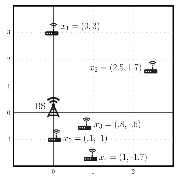
Figure 2: Spatial distribution of devices $\{1,\dots,5\}$ and the base station (BS).

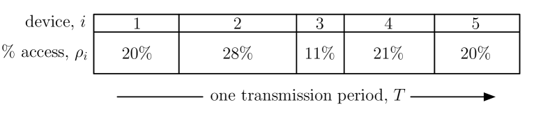
Figure 3: TDMA transmission time allocations for each device.

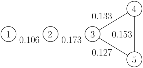
Figure 4: The bargaining graph resulting from the position and TDMA transmission time allocations for each device. Here, we have taken $P_{\max}=3$.

VII Application to multi-user wireless communication

In this section, we provide some simulation results of our proposed Nash bargaining dynamics as applied to a multi-user wireless communication scenario. The scenario we describe here is a simplified version of the one found in [28], and we direct the reader to that reference for a more detailed discussion on the model. We assume that there are $n=5$ single antenna devices distributed spatially in an environment that send data to a fixed base station. We denote the position of device $i\in\{1,\dots,5\}$ as $x_{i}\in\mathbb{R}^{2}$ and we assume without loss of generality that the base station is located at the origin. Figure 2 illustrates the position of the devices. An individual device’s transmission is managed using a time division multiple access (TDMA) protocol. That is, each device $i$ is assigned a certain percentage $\rho_{i}$ of a transmission period of length $T$ in which it is allowed to transmit as specified in Figure 3. We use a commonly used model for the capacity $c_{i}>0$ of the communication channel from device $i$ to the base station, which is a function of their relative distance,

$$c_{i}=\log(1+|x_{i}|^{-1}).$$

In the above, we have taken various physical parameters (such as transmit power constraints, path loss constants, and others) to be $1$ for the sake of presentation. Since $i$ only transmits for $\rho_{i}$ percent of each transmission period, the effective capacity of the channel from device $i$ to base station is $\rho_{i}c_{i}$. It is well-known in wireless communication [29] that multiple antenna devices can improve the channel capacity. Thus, devices $i$ and $j$ may decide to share their data and transmit a multiplexed data signal in both $i$ and $j$’s allocated time slots. In essence, $i$ and $j$ would behave as a single virtual $2$-antenna device. The resulting channel capacity is given by

$$c_{i,j}=\log(1+|x_{i}|^{-1}+|x_{j}|^{-1}),$$

(a) Device allocations

(b) Matching states

Figure 5: Evolution of each device’s allocation and the matching states in dynamics (19). At various times (i.e., $t\approx 4$ and $9$), certain devices change who they identify as partners in the matching which explains the kinks in the trajectories at those times. This occurs because of the evolution of the matching states in (b) and devices cannot correctly deduce the stable matching until $t\approx 9$. The final convergence of the matching states to $\{0,1\}^{|\mathcal{E}|}$ (which we do not show for the sake of presentation) takes much longer than devices need to accurately identify a Nash outcome.

which is greater than both $c_{i}$ and $c_{j}$. However, there is a cost to agent $i$ and $j$ cooperating in this way because their data must be transmitted to each other. We assume that the device-to-device transmissions do not interfere with the device-to-base station transmissions. The power needed to transmit between $i$ and $j$ is given by

$$P_{i,j}=|x_{i}-x_{j}|.$$

If this power is larger than some $P_{\max}>0$, then $i$ and $j$ will not share their data. We can model this scenario via a graph $\mathcal{G}=(\mathcal{V},\mathcal{E},W)$, where $\mathcal{V}=\{1,\dots,5\}$ are the devices, edges correspond to whether or not $i$ and $j$ are willing, based on the power requirements, to share their data

$$(i,j)\in\mathcal{E}\Leftrightarrow P_{i,j}\leq P_{\max},$$

and the edge weights represent the increase in effective channel capacity should devices cooperate,

$$w_{i,j}=(\rho_{i}+\rho_{j})c_{i,j}-\rho_{i}c_{i}-\rho_{j}c_{j},\quad\forall(i,j)\in\mathcal{E}.$$

Figure 4 shows this graph, using the data for the scenario we consider. It is interesting to note that, besides channel capacity and power constraints, one could incorporate other factors into the edge weight definition. For example, if privacy is a concern in the network, then devices may be less likely to share their data with untrustworthy devices which can be modeled by a smaller edge weight.

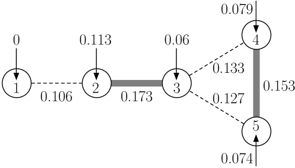
Figure 6: Nash outcome that is distributedly computed by devices. Device matchings are shown by thicker grey edges and allocations to each device are indicated with arrows

TABLE I: Improvements in capacity due to collaboration

	Effective channel	Increase in effective	%
Device	capacity without	channel capacity	improve-
	collaboration, $c_{i}$	in Nash outcome, $\alpha^{b}_{i}$	ment
1	0.288	0	0
2	0.288	0.113	39.2
3	0.693	0.06	8.7
4	0.693	0.079	11.4
5	0.406	0.074	18.2
{1,…,5}	0.441	0.070	15.8

A matching $M$ in the context of this setting corresponds to disjoint pairs of devices that decide to share their data and transmission time slots in order to achieve a higher effective channel capacity. An allocation corresponds to how the resulting improved bit rate is divided between matched devices. For example, if $i$ is allocated an amount of $\alpha^{b}_{i}$, then $i$ and $j$ will transmit their data such that $i$’s data reaches the base station at a rate of $c_{i}+\alpha^{b}_{i}$. The percent improvement in bit rate for $i$ is then given by ${\alpha^{b}_{i}}/{c_{i}}$. Devices use the dynamics (19) to find, in a distributed way, a Nash outcome for this problem. Figure 5 reveals the resulting state trajectories and Figure 6 displays the final Nash outcome. The percent improvements resulting from collaboration for each device are collected in Table I. The last row in this table show that the network-wide improvement is $15.8\%$. Before bargaining, devices $1$ and $2$ have the lowest individual channel capacities and would thus greatly benefit from collaboration. However, due to power constraints, device $1$ can only match with device $2$, who in turn prefers to match with device $3$. This explains why, in the end, device $1$ is left unmatched. Figure 7 illustrates how convergence is still achieved when noise is present in the devices’ dynamics, as forecasted by Corollary VI.3.

Figure 7: When the devices’ dynamics are subjected to noise (normally distributed with zero mean and standard deviation $0.01$), the stable matchings are still correctly deduced and devices’ allocations converge to a neighborhood of the allocations in the Nash outcome.

VIII Conclusions and future work

We have considered bargaining in dyadic-exchange networks, where individual agents decide with whom (if any) to match and agree on an allocation of a common good. For such scenarios, valid notions of outcomes include stable, balanced, and Nash. We have designed provably correct distributed dynamics that asymptotically converge to each of these classes of outcomes. Our technical approach combines graph- and game-theoretic notions with techniques from set-valued dynamics, stability theory, and distributed linear programming. We have illustrated the performance of the proposed coordination algorithm in a wireless communication scenario, where we showed how agent collaborations can, in a fair way, improve both individual and network-wide performance. Future work will include considering other solution concepts on dyadic-exchange networks and applying our techniques to multi-exchange networks (i.e., allowing coalitions of more than two). In addition, we would like to study the rate of convergence and establish more quantifiable robustness properties of balancing dynamics; in particular, the effects of time delays, adversarial agents, and dynamically changing system data. Finally, we wish to apply our dynamics to other coordination tasks and implement them on a multi-agent testbed.

The following result is used in the proof of Proposition V.2 to establish the local stability of each balanced allocation under the dynamics (15).

Lemma .1

(Upper-semicontinuity of the next-best-neighbor sets map). Let $\alpha^{b,*}\in\mathbb{R}^{n}$. Then there exists $\epsilon>0$ such that, for all $(i,j)\in\mathcal{E}$ and all $\|\alpha^{b}-\alpha^{b,*}\|<\epsilon$, the following inclusion holds

$$\texttt{bn}_{{i}\setminus{j}}(\alpha^{b})\subseteq\texttt{bn}_{{i}\setminus{j}}(\alpha^{b,*}).$$

Proof.

Note that, since the number of edges is finite, it is enough to prove that such $\epsilon$ exists for each edge $(i,j)\in\mathcal{E}$ (because then one takes the minimum over all of them). Therefore, let $(i,j)\in\mathcal{E}$ and, arguing by contradiction, assume that for every $\epsilon>0$, there exists $\alpha^{b}$ with $\|\alpha^{b}-\alpha^{b,*}\|<\epsilon$ such that $\texttt{bn}_{{i}\setminus{j}}(\alpha^{b})\not\subseteq\texttt{bn}_{{i}\setminus{j}}(\alpha^{b,*})$. Equivalently, suppose that $\{\alpha^{b,k}\}_{k=1}^{\infty}$ is a sequence converging to $\alpha^{b,*}$ such that, for every $k$, there exists a $\tau^{k}\in\texttt{bn}_{{i}\setminus{j}}(\alpha^{b,k})\setminus\texttt{bn}_{{i}\setminus{j}}(\alpha^{b,*})$. By definition of the next-best-neighbor set, it must be that

$$w_{i,\tau^{k}}-\alpha^{b,k}_{\tau^{k}}\geq w_{i,\tau}-\alpha^{b,k}_{\tau},$$

for all $\tau\in\mathcal{N}(i)\setminus j$. Since $\mathcal{N}(i)\setminus j$ has a finite number of elements, there must be some $\hat{\tau}\in\mathcal{N}(i)$ such that $\tau^{k}=\hat{\tau}$ infinitely often. Therefore, let $\{k_{\ell}\}_{\ell=1}^{\infty}$ be a subsequence such that $\tau^{k_{\ell}}=\hat{\tau}$ for all $\ell$. Then

$$w_{i,\hat{\tau}}-\alpha^{b,k_{\ell}}_{\hat{\tau}}\geq w_{i,\tau}-\alpha^{b,k_{\ell}}_{\tau},$$

for all $\tau\in\mathcal{N}(i)\setminus j$. Taking now the limit as $\ell\rightarrow\infty$,

$$w_{i,\hat{\tau}}-\alpha^{b,*}_{\hat{\tau}}\geq w_{i,\tau}-\alpha^{b,*}_{\tau},$$

for all $\tau\in\mathcal{N}(i)\setminus j$, which contradicts $\hat{\tau}\notin\texttt{bn}_{{i}\setminus{j}}(\alpha^{b,*})$. ∎

References

- [1] W. Ren and R. W. Beard, Distributed Consensus in Multi-vehicle Cooperative Control. Communications and Control Engineering, Springer, 2008.
- [2] F. Bullo, J. Cortés, and S. Martínez, Distributed Control of Robotic Networks. Applied Mathematics Series, Princeton University Press, 2009. Electronically available at http://coordinationbook.info.
- [3] M. Mesbahi and M. Egerstedt, Graph Theoretic Methods in Multiagent Networks. Applied Mathematics Series, Princeton University Press, 2010.
- [4] W. Saad, Z. Han, Z. Debbah, M. Hjørungnes, and T. Başar, “Coalitional game theory for communication networks: A tutorial,” IEEE Signal Processing Magazine, Special Issue on Game Theory, vol. 26, no. 5, pp. 77–97, 2009.
- [5] S. H. Ali, K. Lee, and V. C. M. Leung, “Dynamic resource allocation in OFDMA wireless metropolitan area networks,” IEEE Wireless Communications, vol. 14, pp. 6–13, Feb. 2007.
- [6] Z. Zhaoyang, S. Jing, C. Hsiao-Hwa, M. Guizani, and Q. Peiliang, “A cooperation strategy based on Nash bargaining solution in cooperative relay networks,” IEEE Transactions on Vehicular Technology, vol. 57, pp. 2570–2577, July 2008.
- [7] D. Richert and J. Cortés, “Optimal leader allocation in UAV formation pairs ensuring cooperation,” Automatica, vol. 49, no. 11, pp. 3189–3198, 2013.
- [8] V. Preciado, M. Zargham, C. Enyioha, A. Jadbabaie, and G. Pappas, “Optimal resource allocation for network protection: A geometric programming approach,” IEEE Transactions on Control of Network Systems, vol. 1, pp. 99–108, Mar. 2014.
- [9] M. S. Stankovic, K. H. Johansson, and D. M. Stipanovic, “Distributed seeking of Nash equilibria with applications to mobile sensor networks,” IEEE Transactions on Automatic Control, vol. 57, no. 4, pp. 904–919, 2012.
- [10] C. J. Romanowski, R. Nagi, and M. Sudit, “Data mining in an engineering design environment: OR applications from graph matching,” Computers and Operations Research, vol. 33, pp. 3150–3160, Nov. 2006.
- [11] T. Chakraborty, S. Judd, M. Kearns, and J. Tan, “A behavioral study of bargaining in social networks,” in ACM Conference on Electronic Commerce, pp. 243–252, June 2010.
- [12] A. E. Roth, “The evolution of the labor market for medical interns and residents: A case study in game theory,” Journal of Political Economy, vol. 92, pp. 991–1016, Dec. 1984.
- [13] K. S. Cook and R. M. Emerson, “Power, equity and commitment in exchange networks,” American Sociological Review, vol. 43, pp. 721–739, Oct. 1978.
- [14] D. P. Bertsekas, Network Optimization: Continuous and Discrete Models. Athena Scientific, 1998.
- [15] J. Nash, “The bargaining problem,” Econometrica, vol. 8, no. 2, pp. 155–162, 1950.
- [16] J. Kleinberg and E. Tardos, “Balanced outcomes in social exchange networks,” in Proceedings of the Annual ACM Symposium on Theory of Computing, (Victoria, Canada), pp. 295–304, May 2008.
- [17] M. Bateni, M. Hajiaghayi, N. Immorlica, and H. Mahini, “The cooperative game theory foundations of network bargaining games,” in International Colloquium on Automata, Languages and Programming, (Bordeaux, France), pp. 67–78, July 2010.
- [18] Y. Azar, B. Birnbaum, L. Celis, N. Devanur, and Y. Peres, “Convergence of local dynamics to balanced outcomes,” 2009. Available at http://arxiv.org/abs/0907.4356.
- [19] M. Bayati, C. Borgs, J. Chayes, Y. Kanoria, and A. Montanari, “Bargaining dynamics in exchange networks,” Journal of Economic Theory, 2014. To appear.
- [20] D. P. Bertsekas and J. N. Tsitsiklis, Parallel and Distributed Computation: Numerical Methods. Athena Scientific, 1997.
- [21] M. Burger, G. Notarstefano, F. Bullo, and F. Allgower, “A distributed simplex algorithm for degenerate linear programs and multi-agent assignment,” Automatica, vol. 48, no. 9, pp. 2298–2304, 2012.
- [22] D. Richert and J. Cortés, “Robust distributed linear programming,” IEEE Transactions on Automatic Control, 2013. Submitted. Available at http://carmenere.ucsd.edu/jorge.
- [23] F. H. Clarke, Optimization and Nonsmooth Analysis. Canadian Mathematical Society Series of Monographs and Advanced Texts, Wiley, 1983.
- [24] J. Cortés, “Discontinuous dynamical systems - a tutorial on solutions, nonsmooth analysis, and stability,” IEEE Control Systems Magazine, vol. 28, no. 3, pp. 36–73, 2008.
- [25] S. Boyd and L. Vandenberghe, Convex Optimization. Cambridge University Press, 2004.
- [26] Q. Hui and W. M. Haddad, “Semistability of switched dynamical systems, Part 1: Linear systems theory having a continuum of equilibria,” Nonlinear Analysis: Hybrid Systems, vol. 3, no. 3, pp. 343–353, 2009.
- [27] R. Goebel, R. G. Sanfelice, and A. R. Teel, “Hybrid dynamical systems,” IEEE Control Systems Magazine, vol. 29, no. 2, pp. 28–93, 2009.
- [28] W. Saad, Z. Han, M. Debbah, and A. Hjørungnes, “A distributed coalition formation framework for fair user cooperation in wireless networks,” IEEE Transactions on Wireless Communications, vol. 8, no. 9, pp. 4580–4593, 2009.
- [29] C. Wang, X. Hong, X. Ge, G. Zhang, and J. Thompson, “Cooperative MIMO channel models: A survey,” IEEE Communications Magazine, vol. 48, no. 2, pp. 80–87, 2010.