Proton-Neutron Pairing Amplitude as a Generator Coordinate for Double-Beta Decay

Abstract

We treat proton-neutron pairing amplitudes, in addition to the nuclear deformation, as generator coordinates in a calculation of the neutrinoless double-beta decay of ⁷⁶Ge. We work in two oscillator shells, with a Hamiltonian that includes separable terms in the quadrupole, spin-isospin, and pairing (isovector and isoscalar) channels. Our approach allows larger single-particle spaces than the shell model and includes the important physics of the proton-neutron quasiparticle random-phase approximation (QRPA) without instabilities near phase transitions. After comparing the results of a simplified calculation that neglects deformation with those of the QRPA, we present a more realistic calculation with both deformation and proton-neutron pairing amplitudes as generator coordinates. The future should see proton-neutron coordinates used together with energy-density functionals.

Neutrinoless double-beta ($0\nu\beta\beta$) decay can occur only if neutrinos are Majorana particles. That fact has motivated many expensive and complicated experiments to search for the process. If it is observed, the decay can also reveal an overall neutrino mass scale, $m_{\nu}\equiv\sum_{i}U_{ei}m_{i}^{2}$ (where $i$ labels the mass eigenstates, and $U$ is the neutrino mixing matrix Avignone III et al. (2008)), but only if we know the value of unobservable nuclear matrix elements that play a role in the decay. The entanglement of nuclear and neutrino physics has led nuclear-structure theorists to attempt to calculate the nuclear matrix elements. At present, various nuclear models agree to within factors of about three. More accurate calculations will increase the importance of both existing limits and any actual observation.

The method most often applied to double-beta decay is the proton-neutron (pn) quasiparticle random phase approximation (QRPA). QRPA calculations were the first to suggest that pn pairing quenches double-beta matrix elements Vogel and Zirnbauer (1986); Engel et al. (1988). That result was surprising because evidence for such pairing in spectra and electromagnetic transitions or moments is hard to come by, particularly when the number of neutrons $N$ is significantly larger than the number of protons $Z$, as it is in most nuclei that undergo double-beta decay. At the mean-field level, pn pairing never develops in those nuclei. But the QRPA uncovered pairing fluctuations that have significant effects on both single- and double-beta decay.

Despite this success, the QRPA is not fully realistic because it is built on small oscillations around a single mean field. That means that 1) it is not really suited for complicated but important double-beta-decay parents/daughters such as ⁷⁶Ge and ¹³⁰Xe, in which a single mean field provides a poor representation of the ground state, and 2) its predictions for the effects of pn pairing fluctuations, which are not small, cannot be fully trusted. To treat the physics more reliably, one needs a method in which collective pn pairing fluctuations are allowed to be large. One framework for large-amplitude modes is the generator-coordinate method (GCM) Ring and Schuck (2004); Bender et al. (2003), a variational procedure that works by mixing many mean-field wave functions with varying amounts of collectivity. To treat large-amplitude quadrupole vibrations, for example, it produces a “collective wave function” that superposes Slater determinants (or generalizations) with different amounts of quadrupole deformation in an optimal way. In our work the pn pairing amplitude (defined below) will play the role of collective deformation.

In fact, a sophisticated version of the GCM, in conjunction with energy-density functional theory, has already been applied to double-beta decay Rodríguez and Martínez-Pinedo (2010); Rodríguez and Martinez-Pinedo (2011); Vaquero et al. (2013). The collective coordinates include only axial quadrupole deformation and particle-number fluctuation (from like-particle pairing), however, and so the calculations omit the suppression caused by pn pairing. Not surprisingly, the GCM results tend to be larger than those of e.g. the shell model, which includes pn pairing. If the pn pairing amplitude could be added as another coordinate in these GCM calculations, the matrix elements would probably shrink. No one has ever treated pn pairing as a GCM degree of freedom, however. Because pn pairing is less strongly collective than its like-particle counterpart, doing so requires a careful extension of mean-field methods and the GCM itself. In this paper we undertake that project and report a first application to the $0\nu\beta\beta$ decay of ⁷⁶Ge.

We begin with the matrix elements we wish to calculate. In the closure approximation (which is good to about 10% Pantis and Vergados (1990)), we can write the nuclear $0\nu\beta\beta$ matrix element in terms of the initial and final ground states and a two-body transition operator. If we neglect the “tensor term,” the effect of which is at most 10% Kortelainen and Suhonen (2007); Menéndez et al. (2009), and two-nucleon currents Menéndez et al. (2011) (the effects of which are still uncertain) we can write the matrix element as

$$M^{0\nu} \equiv\bra{F}\hat{M}_{0\nu}\ket{I}=\frac{2R}{\pi g_{A}^{2}}\int_{0}^{\infty}\!\!\!q\,dq$$ (1)

$$\times\bra{F}\sum_{a,b}\frac{j_{0}(qr_{ab})\left[h_{\rm F}(q)+h_{\rm GT}(q)\vec{\sigma}_{a}\cdot\vec{\sigma}_{b}\right]}{q+\overline{E}-(E_{I}+E_{F})/2}\tau^{+}_{a}\tau^{+}_{b}\ket{I}\,,$$

where $\ket{I}$ and $\ket{F}$ are the ground states of the initial and final nuclei, $r_{ab}$ is the distance between nucleons $a$ and $b$, $j_{0}$ is the usual spherical Bessel function, and $R$ is the nuclear radius, inserted by convention to make the matrix element dimensionless. The form factors $h_{\rm F}(q)$ and $h_{\rm GT}(q)$ contain the vector and axial vector coupling constants, forbidden corrections to the weak current, nucleon form factors, and the “Argonne” short-range correlation function Šimkovic et al. (2009). See, e.g., Ref. Šimkovic et al. (2008) for details; note that we absorb the inverse square of the axial-vector coupling constant into our definition of $h_{F}$.

To compute the matrix element in Eq. (1) we need good representations of the initial and final ground states $\ket{I}$ and $\ket{F}$. In this first application to $A=76$ nuclei, we construct the states in a Hilbert space consisting of 36 particles moving freely in the oscillator $fp$ and $sdg$ shells. Our Hamiltonian has the form

$$H =h_{0}-\sum_{\mu=-1}^{1}g^{T=1}_{\mu}\ S^{\dagger}_{\mu}S_{\mu}-\frac{\chi}{2}\sum_{K=-2}^{2}Q^{\dagger}_{2K}Q_{2K}$$

$$-g^{T=0}\sum_{\nu=-1}^{1}P^{\dagger}_{\nu}P_{\nu}+g_{ph}\sum_{\mu,\nu=-1}^{1}F^{\mu{\dagger}}_{\nu}F^{\mu}_{\nu}\,,$$ (2)

where $h_{0}$ contains spherical single particle energies, $Q_{2K}$ are the components of a quadrupole operator defined in Ref. Baranger and Kumar (1968), and

$$S^{\dagger}_{\mu} = \frac{1}{\sqrt{2}}\sum_{l}\hat{l}[c^{\dagger}_{l}c^{\dagger}_{l}]^{001}_{00\mu}\,,\quad P^{\dagger}_{\mu}=\frac{1}{\sqrt{2}}\sum_{l}\hat{l}[c^{\dagger}_{l}c^{\dagger}_{l}]^{010}_{0\mu 0}\,,$$

$$F^{\mu}_{\nu} = \frac{1}{2}\sum_{i}\sigma^{\mu}_{i}\tau^{\nu}_{i}=\sum_{l}\hat{l}[c^{\dagger}_{l}\bar{c}_{l}]^{011}_{0\mu\nu}\,.$$ (3)

In this last equation, $c^{\dagger}_{l}$ is a creation operator, $l$ labels single-particle multiplets with good orbital angular momentum, $\hat{l}\equiv\sqrt{2l+1}$, $S^{\dagger}_{\mu}$ creates a correlated isovector pair with orbital angular momentum $L=0$ and spin $S=0$ (and with $\mu$ labeling the isospin component $T_{z}$), $P^{\dagger}_{\mu}$ creates an isoscalar pn pair with $L=0$ and $S=1$ ($S_{z}=\mu$), and the $F^{\mu}_{\nu}$ are the components of the Gamow-Teller operator. Although the Hamiltonian is not fully realistic, it combines and extends both the $SO(8)$ model Engel et al. (1997); Dussel et al. (1986) and the pairing-plus-quadrupole model Baranger and Kumar (1968); Kisslinger and Sorensen (1963), and contains the most important (collective) parts of shell-model interaction Dufour and Zuker (1996). We discuss the values of the couplings in Eq. (Proton-Neutron Pairing Amplitude as a Generator Coordinate for Double-Beta Decay) shortly.

A direct diagonalization in a space this large is not possible, even with our simple Hamiltonian, and we have already discussed the drawbacks of the QRPA. We therefore turn to the GCM, which has been reviewed in many places (see, e.g., Ref. Ring and Schuck (2004)) and is useful in very-large-scale shell-model problems. The procedure is variational, with an ansatz for the ground state of the form

$$\ket{\Psi}=\sum_{a_{1}a_{2}\ldots a_{n}}f(a_{1},a_{2},\ldots,a_{n})\mathcal{P}\ket{a_{1},a_{2},\ldots,a_{n}}\,.$$ (4)

Here the kets $\ket{a_{1},a_{2},\ldots,a_{n}}$ are mean-field states — Slater determinants or, in our case, quasiparticle vacua — with $n$ expectation values $a_{i}$ specified, $\mathcal{P}$ is an operator that projects onto states with well-defined values for angular momentum and neutron and proton particle numbers, and $f$ is a weight function. The starting point, if we want to include the effects of pn pairing, is a Hartree-Fock-Bogoliubov (HFB) code that mixes neutrons and protons in the quasiparticles, i.e. (schematically):

$$\alpha^{\dagger}\sim u_{p}c^{\dagger}_{p}+v_{p}c_{p}+u_{n}c^{\dagger}_{n}+v_{n}c_{n}\,.$$ (5)

The actual equations contain sums over single particle states as well, so that each of the $u$’s and $v$’s above are replaced by matrices as described, e.g., in Ref. Goodman (1979).

We use the generalized HFB (neglecting the Fock terms in this step) without any symmetry restriction to construct a set of quasiparticle vacua that are constrained to have a particular deformation $\beta$ (defined here as 0.438 fm² MeV^-1 $\chi\braket{Q_{20}}$) and isoscalar-pairing amplitude $\phi=\braket{P_{0}+P_{0}^{\dagger}}/2$ (these are the $a_{i}$ in Eq. (4)), that is, we solve the HFB equations for the Hamiltonian with linear constraints

$$H^{\prime}=H-\lambda_{Z}N_{Z}-\lambda_{N}N_{N}-\lambda_{Q}Q_{20}-\frac{\lambda_{P}}{2}\left(P_{0}+P_{0}^{\dagger}\right)\,,$$ (6)

where the $N_{Z}$ and $N_{N}$ are the proton and neutron number operators — they are part of the usual HFB minimization — and the other $\lambda$’s are Lagrange multipliers to fix the deformation and isoscalar pairing amplitude. (When computing the Fermi part of the $0\nu\beta\beta$ matrix element we substitute the isovector pn operators $(S_{0}-S^{\dagger}_{0})/2i$ for $(P_{0}+P_{0}^{\dagger})/2$ in Eq. (6).) As already noted, without the last multiplier the isoscalar pairing amplitude vanishes unless the strength $g^{T=0}$ of the corresponding interaction is larger than some critical value. For realistic Hamiltonians that is never the case, hence the need to generate amplitudes by force, as it were.

Having obtained a set of HFB vacua with varying amounts of axially symmetric deformation and pn pairing, we project the vacua onto states with the correct number of neutrons and protons and with angular momentum zero. We then solve the Hill-Wheeler equation Ring and Schuck (2004), which amounts to diagonalizing $H$ in the space spanned by our nonorthogonal projected vacua, to determine the weight function $f$ in Eq. (4).

Table 1: Neutron and proton canonical single-particle energies (in MeV) taken from spherical HFB with SkO^′.

	76Ge (n)	76Ge (p)	76Se (n)	76Se (p)
p1/2	-10.31	-6.80	-11.21	-5.06
p3/2	-12.69	-9.56	-13.72	-7.81
f5/2	-9.94	-7.47	-11.08	-5.61
f7/2	-17.63	-15.90	-18.87	-13.95
s1/2	-0.49	6.27	-0.90	7.05
d3/2	1.49	7.94	1.17	8.77
d5/2	-2.60	2.64	-3.26	3.65
g7/2	3.23	6.43	2.24	8.08
g9/2	-8.09	-6.31	-9.31	-4.46

To carry out a fairly realistic calculation, we need appropriate values for the couplings in the Hamiltonian of Eq. (Proton-Neutron Pairing Amplitude as a Generator Coordinate for Double-Beta Decay). We determine them by trying to reproduce the results of calculations with two different Skyrme interactions (SkO^′ Reinhard et al. (1999) and SkM* Bartel et al. (1982)) in ⁷⁶Ge and neighboring nuclei. We first do Skyrme-HFB calculations Stoitsov et al. (2013) in ⁷⁶Ge to determine appropriate volume pairing constants. We then take single-particle energies for each nucleus, which we show for SkO^′ in Table 1, from the results of constrained HFB calculations for ⁷⁶Ge and ⁷⁶Se, which we temporarily force to be spherical. Next we adjust the like-particle part of our isovector pairing interaction ($g_{1}^{T=1}$ and $g_{-1}^{T=1}$) to get the same pairing gaps as the original Skyrme calculations. The resulting occupation numbers are close to the spherical Skyrme-HFB numbers (and, as is typical for such calculations, relatively different from the measured occupations of Refs. Schiffer et al. (2008); Kay et al. (2009)). The Coulomb interaction is not included explicitly in our Hamiltonian, but its effects are present in single-particle energies and the fit isovector pairing interaction.

Next, we fix our quadrupole interaction so that it reproduces the prolate deformation of Skyrme-HFB calculations, now with axial deformation allowed, in ⁷⁶Ge and ⁷⁶Se. The top panel of Fig. 1 compares the diagonal part of the Hamiltonian kernel $\bra{\beta,\phi=0}H\ket{\beta,\phi=0}$ as a function of $\beta$ (we refer this function as a potential energy surface) in the Skyrme HFB and in our model. The lowest minima are prolate in both nuclei. In ⁷⁶Se the surfaces have oblate minima around $\beta=-0.2$ as well, but in general the surfaces are quite flat. (We discuss the bottom part of the figure later.)

Turning to the particle-hole spin-isospin interaction, we take $g_{ph}$ from a deformed Skyrme-QRPA calculation Mustonen et al. (2014), with the relevant piece of the time-odd functional adjusted as in Ref. Bender et al. (2002) to put the Gamow-Teller resonance in ⁷⁶Ge at the correct energy. The resulting values of $g_{ph}$, extracted as in Ref. Sarriguren et al. (1998), are $1.9\times\bar{g}^{T=1}$ for SkO^′ and $0.9\times\bar{g}^{T=1}$ for SkM*, where $\bar{g}^{T=1}$ is the average of the two like-particle pairing strengths. To fix the pn part of our $T=1$ pairing interaction, we adjust $g_{0}^{T=1}$ to make two-neutrino Fermi decay vanish (in the closure approximation); this last step approximates isospin restoration Šimkovic et al. (2013). We find $g_{0}^{T=1}=$ $1.05\times\bar{g}^{T=1}$ for SkO^′ and $0.98\times\bar{g}^{T=1}$, for SkM*.

Figure 1: (Color online.) Upper panels: Potential energy surfaces for SkO^′ (dotted line) and our corresponding model interaction (solid line) at $\phi=0$ with no spin-isospin or isoscalar pairing interactions (together denoted by “pn” in the lower panels) as functions of $\beta$ for ⁷⁶Ge (left) and ⁷⁶Se (right). Lower panels: Potential energy surface from the model without projection and pn at $\phi=0$ (solid red line, same line as in upper figure), with projection but still without pn at $\phi=0$ (dotted blue line), and with both projection and pn at $\phi=3$ (dashed black line). Energy is measured from the unprojected value at $\beta=0$.

That then leaves just the crucial isoscalar pairing strength, $g^{T=0}$. There is no consensus about how best to determine that parameter. We do so by fitting the measured total $\beta^{+}$ strength $B({\rm GT}+)$ from ⁷⁶Se as well as possible. Two separate charge-exchange experiments Helmer et al. (1997); Grewe et al. (2008) have tried to extract $B({\rm GT}+)$. Neither isolates the quantity perfectly but both are consistent with the assumption that $B({\rm GT}+)\approx 1$, and we adopt that value. It is not obvious how much the experimental strength is quenched by states outside the model space, so we always do two fits, one (unquenched) as just described and one (quenched) in which we scale our calculated strength by $(1/1.27)^{2}=0.62$.

Of course, the value we extract for $g^{T=0}$ will depend on our choice of generator coordinates as well as assumptions about quenching. Before turning to the full calculation outlined above we discuss a simpler and more transparent case, in which the quadrupole force is turned off and the isoscalar pairing amplitude (or isovector pn pairing amplitude when we calculate the Fermi matrix element) is the sole coordinate. Though the isoscalar pairs create a spin vector that always breaks rotational symmetry and forces us to do angular-momentum projection, the absence of a quadrupole force makes both the initial and final nuclear densities nearly spherical. The main advantage of spatial spherical symmetry is that we can compare the results with those of the spherical QRPA, for which we developed a code.

With a single generator coordinate and the interaction we extract from SkO^′ (minus the quadrupole part), there is no value of $g^{T=0}$ for which $B({\rm GT}+)$ from ⁷⁶Se is as small as 1, much less 0.62; we therefore let $g^{T=0}=1.47\times\bar{g}^{T=1}$, the value for which $B({\rm GT}+)$ is the smallest. With the interaction we extract from SkM*, whether we quench our strength or not, there are two values of $g^{T=0}$ that produce the correct $\beta^{+}$ strength — 0.82 and 1.56 (unquenched) or 0.33 and 1.77 (quenched), all in units of $\bar{g}^{T=1}$ — and we choose the larger value in each case. With all parameters finally determined, we can calculate the $0\nu\beta\beta$ matrix element; Table 2 displays the results at various stages of approximation.

In our QRPA calculation, we adjust $g^{T=0}$ (commonly called $g_{pp}$ when divided by $\bar{g}^{T=1}$) in exactly the same way. The values we obtain are only slightly different. The last column of Table 2 contains the QRPA $0\nu\beta\beta$ matrix elements. They are fairly close to those of the GCM calculation, but much more sensitive to $g^{T=0}$.

Table 2: The $0\nu\beta\beta$ matrix element $M^{0\nu}$ for the decay of ⁷⁶Ge in a simplified calculation that neglects deformation, at various levels of approximation. The first column contains the source of the couplings in Eq. (Proton-Neutron Pairing Amplitude as a Generator Coordinate for Double-Beta Decay), the second the matrix element when the spin-isospin and isoscalar pairing interactions are absent, the third the matrix element with only isoscalar pairing missing, the fourth the full GCM result, and the last the result of the QRPA with the same Hamiltonian (except for a slightly modified $g^{T=0}$). The matrix elements in parentheses are obtained by quenching our $B({\rm GT}+)$.

Skyrme	no $g_{ph},g^{T=0}$	no $g^{T=0}$	full	QRPA
SkO′	14.0	9.5	5.4 (5.4)	5.6 (5.0)
SkM*	11.8	9.4	4.1 (2.8)	3.5 (2.5)

To clarify this last statement, we show the GCM and QRPA matrix elements as functions of $g^{T=0}/\bar{g}^{T=1}$ in Fig. 2. The QRPA curves lie slightly above their GCM counterparts until $g^{T=0}/\bar{g}^{T=1}$ reaches a critical value slightly larger than 1.5; at that point a mean-field phase transition from an isovector pair condensate to an isoscalar condensate causes the famous QRPA “collapse.” The collapse is spurious, as the GCM results show. Its presence in mean-field theory makes the QRPA unreliable near the critical point. It is actually a bit of a coincidence that the QRPA matrix elements in the table are as close as they are to those of the GCM; a small change in $g^{T=0}$ would affect them substantially (though because it also alters $B({\rm GT}+)$ a lot, fitting to $B({\rm GT}+)=0.62$ rather than 1.0 does not have a huge effect on the $0\nu\beta\beta$ matrix element). The GCM result is not only better behaved near the critical point but also, we believe, quite accurate. In the $SO(8)$ model used to test many-body methods in $\beta\beta$ decay many times, the GCM result is nearly exact for all $g^{T=0}$. That is not the case for extensions of the QRPA that attempt to ameliorate its shortcomings Toivanen and Suhonen (1995); Rodin and Faessler (2002), though some of those work better around the phase transition than others.

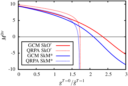
Figure 2: (Color online.) Dependence of the GCM (solid) and QRPA (dashed) $0\nu\beta\beta$ matrix elements on the strength $g^{T=0}$ of the isoscalar pairing interaction. The red (upper) and blue (lower) lines of each type correspond to the interaction parameters extracted from SkO^′ and SkM*. The divergence in the QRPA near $g^{T=0}/\bar{g}^{T=1}=1.5$ is discussed in the text.

To show why the GCM behaves well, we display in the bottom right part of Fig. 3 the quantity $\mathcal{N}_{\phi_{I}}\mathcal{N}_{\phi_{F}}\bra{\phi_{F}}\mathcal{P}_{F}\hat{M}_{0\nu}\mathcal{P}_{I}\ket{\phi_{I}}$, where $\ket{\phi_{I}}$ is a quasiparticle vacuum in ⁷⁶Ge constrained to have isoscalar pairing amplitude $\phi_{I}$, $\phi_{F}$ is an analogous state in ⁷⁶Se, $\mathcal{P}_{I}$, $\mathcal{P}_{F}$ project onto states with angular momentum zero and the appropriate values of $Z$ and $N$, and $\mathcal{N}_{\phi_{I}},\mathcal{N}_{\phi_{F}}$ normalize the projected states. This quantity is the contribution to the $0\nu\beta\beta$ matrix element from states with particular values of the initial and final isoscalar pairing amplitudes. The contribution is positive around zero condensation in the two nuclei and negative when the final pairing amplitude is large. Thus the GCM states must contain components with significant pn pairing when $g^{T=0}$ is near its fit value. The appearance of this plot is different from those in which the matrix element is plotted versus initial and final deformation Rodríguez and Martínez-Pinedo (2010); Rodríguez and Martinez-Pinedo (2011); Vaquero et al. (2013). Here the matrix element is small or negative even if the initial and final pairing amplitudes have the same value, as long as that value is large. The behavior reflects the qualitatively different effects of isovector and isoscalar pairs on the matrix element Engel et al. (1988), effects that have no analog in the realm of deformation.

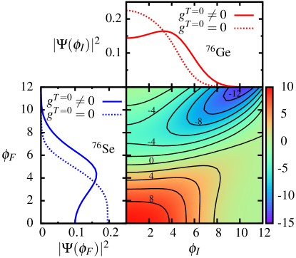
Figure 3: (Color online.) Bottom right: $\mathcal{N}_{\phi_{I}}\mathcal{N}_{\phi_{F}}\bra{\phi_{F}}\mathcal{P}_{F}\hat{M}_{0\nu}\mathcal{P}_{I}\ket{\phi_{I}}$ for projected quasiparticle vacua with different values of the initial and final isoscalar pairing amplitudes $\phi_{I}$ and $\phi_{F}$, from the SkO^′-based interaction (see text). Top and bottom left: Square of collective wave functions in ⁷⁶Ge and ⁷⁶Se.

The weight function $f$ in the GCM ansatz multiplies non-orthogonal states and so is not really a “collective ground-state wave function.” The object that does play that role for is a member of an orthogonalized set defined, e.g., in Refs. Ring and Schuck (2004) and Rodríguez and Martinez-Pinedo (2011). The top and left parts of Fig. 3 show the square of this collective wave function for ⁷⁶Ge and ⁷⁶Se, with $g^{T=0}$ set both to zero and the fit value. It is clear in both nuclei, but particularly in ⁷⁶Se, that the isoscalar pairing interaction pushes the wave function into regions of large $\phi$, where the matrix element in the bottom right panel is significantly reduced. It is also clear that for $g^{T=0}\neq 0$ the collective wave functions are far from the Gaussians that one would obtain in the harmonic (QRPA) approximation. Isoscalar pairing really is, and must be treated as, a large-amplitude mode.

We turn finally to the more realistic calculation that includes both deformation and the pn pairing amplitude as generator coordinates. We fit the couplings in $H$ just as described earlier; the strength of the quadrupole interaction no longer vanishes and some of the other parameters change slightly: $g_{0}^{T=1}=0.90$ for the interaction based on SkO^′ and 0.79 for that based on SkM*, and $g^{T=0}=1.75$ for SkO^′ and 1.51 for SkM*, in units of $\bar{g}^{T=1}$. The calculated $B({\rm GT}+)$ in both cases is larger than the experimental data with or without quenching, which therefore does not alter the value of $g^{T=0}$.

First we analyze the influence of the number and angular-momentum projection on energy. The bottom part of Fig. 1 shows the projected potential energy surfaces $\bra{\beta,\phi}\mathcal{P}H\mathcal{P}\ket{\beta,\phi}$ for two values of $\phi$, along with the unprojected surface from the top part of the panel. Projecting at $\phi=0$ without including pn interactions, the figure shows, lowers the energy by several MeV. The correlation energy from the angular momentum projection is large in the deformed regions, and projection causes both the oblate and prolate configurations that are low lying before projection to become clear minima.

With the pn interactions included, we present the surface at $\phi=3$, where the collective wave function peaks, rather than at $\phi=0$. The curve is shifted up by the repulsive spin-isospin interaction and downward by the isoscalar pairing, so that the final location depends on the relative sizes of $g_{ph}$ and $g^{T=0}$. The SkO^′-based interaction has a particularly large $g_{ph}$ and so the final curve is higher than the initial unprojected curve without the pn terms. The curves flatten and in ⁷⁶Se the oblate minimum becomes the lowest.

Table 3: GCM ground state energies, in MeV, with both deformation and isoscalar pairing as generator coordinates. The energies are measured from the energy of the state with $\beta=0$, $\phi=0$, $g_{ph}=g^{T=0}=0$ and no projection.

	SkO′		SkM*
	76Ge	76Se	76Ge	76Se
no $g_{ph},g^{T=0}$	-6.0	-8.1	-5.5	-7.1
no $g^{T=0}$	+10.5	+6.6	+2.1	-0.9
full	-0.9	-6.9	-7.7	-12.4

Table 3 shows the GCM correlation energies themselves with successively more pn interaction included. The spin-isospin term in the Hamiltonian increases the energies by about 15 MeV for the SkO^′-based interaction, which again, is quite strong in that channel, and 8 MeV for the SkM*-based interaction. The isoscalar pairing interaction then decreases the energy by 10–13 MeV, depending on the nucleus and interaction.

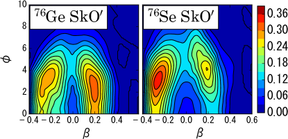
Figure 4: (Color online.) Square of the collective wave functions in the calculation that includes deformation, in ⁷⁶Ge (left) and ⁷⁶Se (right), for the SkO^′-based interaction.

Finally, Fig. 4 shows the squares of the collective wave functions in $\beta$ and $\phi$. These wave functions closely mirror the projected potential energy surfaces. As in the example without deformation, the peaks are at nonzero isoscalar-pairing amplitude. Regarding deformation, the largest peak is in the prolate region for ⁷⁶Ge and in the oblate region for ⁷⁶Se. Though that is also the case in the calculations of Refs. Rodríguez and Martínez-Pinedo (2010); Rodríguez and Martinez-Pinedo (2011); Vaquero et al. (2013), our wave functions are still quite different from the ones in those papers, and our matrix element is less suppressed. The full result of our calculation is $M^{0\nu}=4.7$, with both the SkO^′- and SkM*-based interactions. The number breaks down into 3.4 from the Gamow-Teller operator and 1.2 from the Fermi operator for SkO^′, and 3.7 from the Gamow-Teller operator and 1.0 from the Fermi operator for SkM*.

In summary, the ease with which the GCM works in a large model space, even with several coordinates, means that it can include physics that is beyond the shell model. And because it mixes mean fields and has no issues with phase transitions, it offers a more comprehensive and accurate treatment of correlations than does the QRPA. One direction for future research in the pn GCM is a more complete effective interaction in multi-shell model spaces; another, perhaps more important, is an implementation together with Skyrme and Gogny energy-density functionals or with their successors. The combination of projection and GCM with density-functional theory poses a few conceptual problems (see, e.g., Ref. Bender et al. (2011)) but recent progress suggests that they will be resolved before too long. The inclusion of pn degrees of freedom as generator coordinates should soon improve the quality of density-functional-based double-beta matrix elements.

We gratefully acknowledge useful discussions with T. R. Rodríguez. This work was supported by the U.S. Department of Energy through Contract No. DE-FG02-97ER41019, and JUSTIPEN (Japan-U.S. Theory Institute for Physics with Exotic Nuclei) under Grant No. DE-FG02-06ER41407 (U. Tennessee). We used computational resources at the National Institute for Computational Sciences (http://www.nics.tennessee.edu/).

References

- Avignone III et al. (2008) F. T. Avignone III, S. R. Elliott, and J. Engel, Rev. Mod. Phys. 80, 481 (2008).
- Vogel and Zirnbauer (1986) P. Vogel and M. R. Zirnbauer, Phys. Rev. Lett. 57, 3148 (1986).
- Engel et al. (1988) J. Engel, P. Vogel, and M. R. Zirnbauer, Phys. Rev. C 37, 731 (1988).
- Ring and Schuck (2004) P. Ring and P. Schuck, The Nuclear Many-Body Problem, Texts and Monographs in Physics (Springer, 2004).
- Bender et al. (2003) M. Bender, P.-H. Heenen, and P.-G. Reinhard, Rev. Mod. Phys. 75, 121 (2003).
- Rodríguez and Martínez-Pinedo (2010) T. R. Rodríguez and G. Martínez-Pinedo, Phys. Rev. Lett. 105, 252503 (2010).
- Rodríguez and Martinez-Pinedo (2011) T. R. Rodríguez and G. Martinez-Pinedo, Prog. Part. Nucl. Phys. 66, 436 (2011).
- Vaquero et al. (2013) N. L. Vaquero, T. R. Rodríguez, and J. L. Egido, Phys. Rev. Lett. 111, 142501 (2013).
- Pantis and Vergados (1990) G. Pantis and J. Vergados, Phys. Lett. B 242, 1 (1990).
- Kortelainen and Suhonen (2007) M. Kortelainen and J. Suhonen, Phys. Rev. C 75, 051303(R) (2007).
- Menéndez et al. (2009) J. Menéndez, A. Poves, E. Caurier, and F. Nowacki, Nucl. Phys. A 818, 139 (2009).
- Menéndez et al. (2011) J. Menéndez, D. Gazit, and A. Schwenk, Phys. Rev. Lett. 107, 062501 (2011).
- Šimkovic et al. (2009) F. Šimkovic, A. Faessler, H. Müther, V. Rodin, and M. Stauf, Phys. Rev. C 79, 055501 (2009).
- Šimkovic et al. (2008) F. Šimkovic, A. Faessler, V. Rodin, P. Vogel, and J. Engel, Phys. Rev. C 77, 045503 (2008).
- Baranger and Kumar (1968) M. Baranger and K. Kumar, Nucl. Phys. A 110, 490 (1968).
- Engel et al. (1997) J. Engel, S. Pittel, M. Stoitsov, P. Vogel, and J. Dukelsky, Phys. Rev. C 55, 1781 (1997).
- Dussel et al. (1986) G. Dussel, E. Maqueda, R. Perazzo, and J. Evans, Nucl. Phys. A 460, 164 (1986).
- Kisslinger and Sorensen (1963) L. S. Kisslinger and R. A. Sorensen, Rev. Mod. Phys. 35, 853 (1963).
- Dufour and Zuker (1996) M. Dufour and A. P. Zuker, Phys. Rev. C 54, 1641 (1996).
- Goodman (1979) A. L. Goodman, Advances in Nuclear Physics, edited by J. V. Negele and E. Vogt, Vol. 11 (Plenum Press, New York, 1979) p. 263.
- Reinhard et al. (1999) P.-G. Reinhard, D. J. Dean, W. Nazarewicz, J. Dobaczewski, J. A. Maruhn, and M. R. Strayer, Phys. Rev. C 60, 014316 (1999).
- Bartel et al. (1982) J. Bartel, P. Quentin, M. Brack, C. Guet, and H.-B. Håkansson, Nucl. Phys. A 386, 79 (1982).
- Stoitsov et al. (2013) M. Stoitsov, N. Schunck, M. Kortelainen, N. Michel, H. Nam, E. Olsen, J. Sarich, and S. Wild, Comput. Phys. Commun. 184, 1592 (2013).
- Schiffer et al. (2008) J. P. Schiffer, S. J. Freeman, J. A. Clark, C. Deibel, C. R. Fitzpatrick, S. Gros, A. Heinz, D. Hirata, C. L. Jiang, B. P. Kay, A. Parikh, P. D. Parker, K. E. Rehm, A. C. C. Villari, V. Werner, and C. Wrede, Phys. Rev. Lett. 100, 112501 (2008).
- Kay et al. (2009) B. P. Kay, J. P. Schiffer, S. J. Freeman, T. Adachi, J. A. Clark, C. M. Deibel, H. Fujita, Y. Fujita, P. Grabmayr, K. Hatanaka, D. Ishikawa, H. Matsubara, Y. Meada, H. Okamura, K. E. Rehm, Y. Sakemi, Y. Shimizu, H. Shimoda, K. Suda, Y. Tameshige, A. Tamii, and C. Wrede, Phys. Rev. C 79, 021301 (R) (2009).
- Mustonen et al. (2014) M. T. Mustonen, T. Shafer, Z. Zenginerler, and J. Engel, Phys. Rev. C 90, 024308 (2014).
- Bender et al. (2002) M. Bender, J. Dobaczewski, J. Engel, and W. Nazarewicz, Phys. Rev. C 65, 054322 (2002).
- Sarriguren et al. (1998) P. Sarriguren, E. M. de Guerra, A. Escuderos, and A. C. Carrizo, Nucl. Phys. A 635, 55 (1998).
- Šimkovic et al. (2013) F. Šimkovic, V. Rodin, A. Faessler, and P. Vogel, Phys. Rev. C 87, 045501 (2013).
- Helmer et al. (1997) R. L. Helmer, M. A. Punyasena, R. Abegg, W. P. Alford, A. Celler, S. El-Kateb, J. Engel, D. Frekers, R. S. Henderson, K. P. Jackson, S. Long, C. A. Miller, W. C. Olsen, B. M. Spicer, A. Trudel, and M. C. Vetterli, Phys. Rev. C 55, 2802 (1997).
- Grewe et al. (2008) E.-W. Grewe, C. Bäumer, H. Dohmann, D. Frekers, M. N. Harakeh, S. Hollstein, H. Johansson, L. Popescu, S. Rakers, D. Savran, H. Simon, J. H. Thies, A. M. van den Berg, H. J. Wörtche, and A. Zilges, Phys. Rev. C 78, 044301 (2008).
- Toivanen and Suhonen (1995) J. Toivanen and J. Suhonen, Phys. Rev. Lett. 75, 410 (1995).
- Rodin and Faessler (2002) V. Rodin and A. Faessler, Phys. Rev. C 66, 051303 (2002).
- Bender et al. (2011) M. Bender, T. Duguet, P.-H. Heenen, and D. Lacroix, Int. J. Mod. Phys. E 20, 259 (2011).