The Maslov index in symplectic Banach spaces

Abstract.

We consider a curve of Fredholm pair!of Lagrangian subspaces!curveFredholm pairs of Lagrangian subspacesLagrangian subspaces in a fixed Symplectic form!weak Banach space!with varying weak symplectic structureBanach space with continuously varying weak symplectic structures. Assuming vanishing index, we obtain intrinsically a continuously varying splitting of the total Banach space into pairs of symplectic subspaces. Using such decompositions we define the Maslov index of the curve by symplectic reduction to the classical finite-dimensional case. We prove the transitivity of repeated symplectic reductions and obtain the invariance of the Maslov index under Symplectic reduction symplectic reduction, while recovering all the standard properties of the Maslov index.

As an application, we consider curves of elliptic operators which have varying Principal symbolprincipal symbol, varying Domain!maximalmaximal domain and are Elliptic differential operators!of not-Dirac typenot necessarily of Dirac type. For this class of operator curves, we derive a desuspension spectral flow formula for varying well-posed boundary conditions on manifolds with boundary and obtain the splitting of the spectral flow on Partitioned manifoldpartitioned manifolds.

Preface

The purpose of this Memoir is to establish a universal relationship between incidence geometries in finite and infinite dimensions. In finite dimensions, counting incidences is nicely represented by the Maslov index. It counts the dimensions of the intersections of a pair of curves of Lagrangian subspaces in a symplectic finite-dimensional vector space. The concept of the Maslov index is non-trivial: in finite dimensions, the Maslov index of a loop of pairs of Lagrangians does not necessarily vanish. In infinite dimensions, counting incidences is nicely represented by the spectral flow. It counts the number of intersections of the spectral lines of a curve of self-adjoint Fredholm operators with the zero line. In finite dimensions, the spectral flow is trivial: it vanishes for all loops of Hermitian matrices.

Over the last two decades there have been various, and in their way successful attempts to generalize the concept of the Maslov index to curves of Fredholm pairs of Lagrangian subspaces in strongly symplectic Hilbert space, to establish the correspondence between Lagrangian subspaces and self-adjoint extensions of closed symmetric operators, and to prove spectral flow formulae in special cases, namely for curves of Dirac type operators and other curves of closed symmetric operators with bounded symmetric perturbation and subjected to curves of self-adjoint Fredholm extensions (i.e., well-posed boundary conditions). While these approaches vary quite substantially, they all neglect the essentially finite-dimensional character of the Maslov index, and, consequently, break down when one deals with operator families of varying maximal domain. Quite simply, there is no directly calculable Maslov index when the symplectic structures are weak (i.e., the symplectic forms are not necessarily generated by anti-involutions $J$) and vary in an uncontrolled way.

In this Memoir we show a way out of this dilemma. We develop the classical method of symplectic reduction to yield an intrinsic reduction to finite dimension, induced by a given curve of Fredholm pairs of Lagrangians in a fixed Banach space with varying symplectic forms. From that reduction, we obtain an intrinsic definition of the Maslov index in symplectic Banach bundles over a closed interval. This Maslov index is calculable and yields a general spectral flow formula. In our application for elliptic systems, say of order one on a manifold $M$ with boundary $\Sigma$, our fixed Banach space (actually a Hilbert space) is the Sobolev space $H^{1/2}(\Sigma;E|_{\Sigma})$ of the traces at the boundary of the $H^{1}(M;E)$ sections of a Hermitian vector bundle $E$ over the whole manifold. For $H^{1/2}(\Sigma;E|_{\Sigma})$, we have a family of continuously varying weak symplectic structures induced by the principal symbol of the underlying curve of elliptic operators, taken over the boundary in normal direction. That yields a symplectic Banach bundle which is the main subject of our investigation.

Whence, the message of this Memoir is: The Maslov index belongs to finite dimensions. Its most elaborate and most general definitions can be reduced to the finite-dimensional case in a natural way. The key for that - and for its identification with the spectral flow - is the concept of Banach bundles with weak symplectic structures and intrinsic symplectic reduction. From a technical point of view, that is the main achievement of our work.

Bernhelm Booß-Bavnbek
Chaofeng Zhu

Introduction

Upcoming and continuing interest in the Maslov index

Since the legendary work of Maslov, V.P.V.P. Maslov [66] in the mid 1960s and the supplementary explanations by Arnol’d, V.IV. Arnol’d [3], there has been a continuing interest in the Maslov indexMaslov index for Continuously varying!Fredholm pairs of Lagrangian subspacescurves of pairs of Lagrangians in symplectic space. As explained by Maslov and Arnol’d, the interest arises from the study of Dynamical systemsdynamical systems in classical mechanics and related problems in Morse theoryMorse theory. This same index occurs as well in certain asymptotic formulae for solutions of the Schrödinger equations. For a systematic review of the basic vector analysis and geometry and for the physics background, we refer to Arnol’d, V.IArnol’d [4] and de Gosson, M.M. de Gosson [40].

The Morse theory!Morse index theoremMorse index theorem expresses the Morse index of a geodesic by the Maslov index. Later, Yoshida, T.T. Yoshida [103] and Nicolaescu, L.L. Nicolaescu [76, 77] expanded the view by embracing also spectral problems for Elliptic differential operators!Dirac type operatorsDirac type operators on Partitioned manifoldpartitioned manifolds and thereby stimulating some quite new research in that direction. For a short review, we refer to our Section 4.1 below.

Weak symplectic forms on Banach manifolds

Early in the 1970s, Chernoff, P.R.Marsden, J.E.P. Chernoff, J. Marsden [35] and Weinstein, A.A. Weinstein [99] called attention to the practical and theoretical importance of Banach manifold!symplectic forms on itsymplectic forms on Banach manifolds. See Swanson, R.C.R.C. Swanson [92, 93, 94] for an elaboration of the achievements of that period regarding Banach space!linear symplectic structures on itlinear symplectic structures on Banach spaces. It seems, however, that rigorous and operational definitions of the Maslov index of Continuously varying!Fredholm pairs of Lagrangian subspacescurves of Lagrangian subspaces!in spaces of infinite dimensionLagrangian subspaces in spaces of infinite dimension was not obtained until 25 years later. Our Booß–Bavnbek, B.Zhu, C.[25, Section 3.2] gives an account and compares the various definitions.

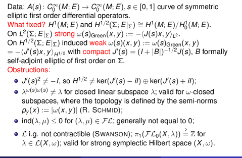
Figure 0.1. Why going weak and what obstructions to circumvent?

Swanson, R.C.Schmid, R.J@$J$ operator associated to symplectic formOperator!associated to symplectic formSymplectic form!associated almost complex generating operatorObstructions to straight forward generalization!generator $J$ non-invertible Obstructions to straight forward generalization!no symplectic splitting Obstructions to straight forward generalization!double annihilator not the identity on closed subspaces Obstructions to straight forward generalization!non-vanishing index of Fredholm pair of Lagrangian subspaces Obstructions to straight forward generalization!${\mathcal{L}}$ not contractibleObstructions to straight forward generalization!fundamental group of Fredholm Lagrangian Grassmannian unknownObstructions to straight forward generalization!no meaningful Maslov cycleFredholm Lagrangian Grassmannian

At the same place we emphasized a couple of rather serious obstructions (see Figure 0.1) to applying these concepts to arbitrary systems of Elliptic differential operators!of non-Dirac typeelliptic differential equations of non-Dirac type: Firstly, some of the key section spaces for studying Boundary value problemsboundary value problems (the Sobolev spaces!with weak symplectic formsSobolev space H@$H^{1/2}(\Sigma;E\mid_{\Sigma})$ weak symplectic Sobolev space$H^{1/2}(\Sigma;E|_{\Sigma})$ containing the traces over the boundary $\Sigma=\partial M$ of sections over the whole manifold M@$M,M(s)$ smooth compact manifold!with boundary $\Sigma,\Sigma(s)$$M$) are not carrying a Symplectic form!strongstrong symplectic structure, but are naturally equipped with a Symplectic form!weakweak structure not admitting the rule J@$J$ operator associated to symplectic formOperator!associated to symplectic formSymplectic form!associated almost complex generating operator $J^{2}=-I$. Secondly, in Booß–Bavnbek, B.Zhu, C.[25] our definition of the Maslov index in weak symplectic spaces requires a Symplectic splittingsymplectic splitting which does not always exist, is not canonical, and therefore, in general, not obtainable in a continuous way for continuously varying symplectic structures. Recall that a symplectic splitting of a symplectic Banach space $(X,\omega)$ is a decomposition $X=X^{-}\oplus X^{+}$ with $-i\omega$ negative, respectively, positive definite on $X^{\mp}$ and vanishing on $X^{-}\times X^{+}$. Thirdly, a priori, a Symplectic reduction!finite-dimensionalsymplectic reduction to finite dimensions is not obtainable for weak symplectic structures in the setting of [25].

An additional incitement to investigate weak symplectic structures comes from a stunning observation of Witten, E.E. Witten (explained by Atiyah, M.F.M.F. Atiyah in [5] in a heuristic way). He considered a weak presymplectic form on the loop space M@$\operatorname{Map}(S^{1},M)$ loop spaceGeodesic!loop space of a manifold$\operatorname{Map}(S^{1},M)$ of a finite-dimensional closed orientable Riemannian manifold $M$ and noticed that a (future) thorough understanding of the infinite-dimensional symplectic geometry of that loop space “should lead rather directly to the Index!Atiyah-Singer Index Theorem!via infinite-dimensional symplectic geometryindex theorem for Dirac operators” (l.c., p. 43). Of course, restricting ourselves to the linear case, i.e., to the geometry of Lagrangian subspaces instead of Lagrangian manifoldLagrangian manifolds, we can only marginally contribute to that program in this Memoir.

Symplectic reduction

Symplectic reduction!history, origin and meaning In their influential paper [65, p. 121], Marsden, J.E.Weinstein, A.J. Marsden and A. Weinstein describe the purpose of symplectic reduction in the following way:

“… when we have a Symplectic geometry!symplectic manifoldsymplectic manifold on which a group acts symplectically, we can reduce this Symplectic reduction!reduced phase spacephase space to another symplectic manifold in which, roughly speaking, the symmetries are divided out.”

and

“When one has a Hamiltonian systemHamiltonian system on the phase space which is invariant under the group, there is a Hamiltonian system canonically induced on the reduced phase space.”

The basic ideas go back to the work of Hamel, G.G. Hamel [54, 55] and Carathéodory, C.C. Carathéodory [33] in Dynamical systemsdynamical systems at the beginning of the last century, see also Souriau, J.-M.J.-M. Souriau [91]. For Symplectic reduction!in low-dimensional geometrysymplectic reduction in low-dimensional geometry see the monographs by Donaldson, S.K.Kronheimer, P.B.S.K. Donaldson and P.B. Kronheimer, and by McDuff, D.Salamon, D.D. McDuff and D. Salamon [42, 68].

Our aim is less intricate, but not at all trivial: Following Nicolaescu, L.L. Nicolaescu [77] and Booß–Bavnbek, B.Furutani, K.K. Furutani [18] (joint work with the first author) we are interested in the finite-dimensional reduction of Fredholm pair!of Lagrangian subspacesFredholm pairs of Lagrangian linear subspaces in infinite-dimensional Banach space. The Symplectic reduction!general proceduregeneral procedure is well understood, see also Kirk, P.Lesch, M.P. Kirk and M. Lesch in [60, Section 6.3]: let $W\subset X$ be a closed Co-isotropic subspacesco-isotropic subspace of a symplectic Banach space X@$(X,\omega)$ symplectic vector or Banach space$(X,\omega)$. Then W@$W/W^{\omega}$ reduced symplectic space$W/W^{\omega}$ inherits a symplectic form from $\omega$ such that

$${R@R_{W}(\lambda)symplecticreductionofisotropic\lambda alongco-isotropicW}R_{W}(\lambda)\ :=\ \frac{(\lambda+W^{\omega})\cap W}{W^{\omega}}\ \subset\ \frac{W}{W^{\omega}}\text{ isotropic for $\lambda$ isotropic}.$$

Here $W^{\omega}$ denotes the annihilator of $W$ with respect to the symplectic form $\omega$ (see Definition 1.2.1c).

In general, however, the reduced space $R_{W}(\lambda)$ does not need to be Lagrangian in $W/W^{\omega}$ even for Lagrangian $\lambda$ unless we have $W^{\omega}\subset\lambda\subset W$ (see Proposition 1.4.8). In Nicolaescu, L.Booß–Bavnbek, B.Furutani, K.[77, 18] a closer analysis of the Symplectic reduction!reduction mapreduction map $R_{W}$ is given within the setting of strong symplectic structures; with emphasis on the topology of the space of Fredholm pairs of Lagrangians; and for fixed $W$. Now we drop the restriction to strong symplectic forms; our goal is to define the Maslov index for Continuously varying!Fredholm pairs of Lagrangian subspacescontinuous Fredholm pair!of Lagrangian subspaces!curvecurves $s\to(\lambda(s),\mu(s))$ of Fredholm pairs of Lagrangians with respect to continuously varying symplectic forms $\omega(s)$; and, at least locally (for $s\in(t-\varepsilon,t+\varepsilon)$ around $t\in[0,1]$), we let the pair $(\lambda(t),\mu(t))$ induce the reference space $W(t)$ for the Symplectic reductionsymplectic reduction and the pair $(\lambda(s),\mu(s))$ induce the reduction map $R^{(s)}_{W(t)}$ in a natural way. The key to finding the reference spaces $W(t)$ and defining a suitable reduction map $R_{W(t)}$ is our Proposition 1.3.3. It is on decompositions of symplectic Banach spaces, naturally induced by a given Fredholm pair of Lagrangians of vanishing index. It might be, as well, of independent interest. The assumption of vanishing index is always satisfied for Fredholm pairs of Lagrangian subspaces in strong symplectic Hilbert spaces, and by additional global analysis arguments in our applications as well.

Thus for each path $\{(\lambda(s),\mu(s))\}_{s\in[0,1]}$ of Fredholm pairs of Lagrangian subspaces of vanishing index, we receive a finite-dimensional symplectic reduction intrinsically, i.e., without any other assumption. The reduction transforms the given path into a path of pairs of Lagrangians in finite-dimensional symplectic space. The main part of the Memoir is then to prove the invariance under symplectic reduction and the independence of choices made. That permits us a conservative view in this Memoir. Instead of defining the Maslov index in infinite dimensions via spectral theory of unitary generators of the Lagrangians as we did in Booß–Bavnbek, B.Long, Y.Zhu, C.[25], we elaborate the concept of the Maslov index!in finite dimensionsMaslov index in finite dimensions and reduce the infinite-dimensional case to the finite-dimensional case, i.e., we take the symplectic reduction as our beginning for re-defining the Maslov index instead of deploring its missing.

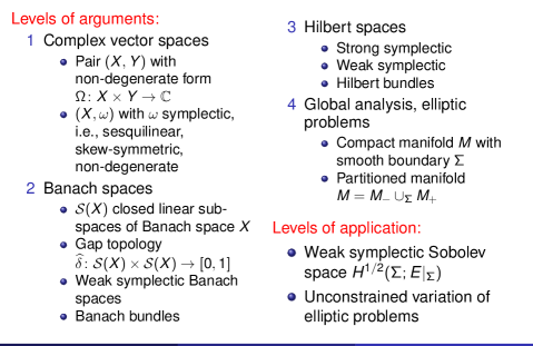
Figure 0.2. Natural levels of treatment

Levels of treatment

Structure of presentation

This Memoir is divided into four chapters and one appendix. The first three chapters present a rigorous definition of the Maslov index in Banach bundles by symplectic reduction. In Chapter 1, we fix the notation and establish our key technical device, namely the mentioned Banach space!natural decompositionnatural decomposition of a symplectic Banach space into two symplectic spaces, induced by a pair of co-isotropic subspaces with finite codimension of their sum and finite dimension of the intersection of their annihilators. We introduce the Symplectic reductionsymplectic reduction of arbitrary linear subspaces via a fixed co-isotropic subspace $W$ and prove the transitivity of the symplectic reduction when replacing $W$ by a larger co-isotropic subspace $W^{\prime}$. For Fredholm pairs of Lagrangian subspaces of vanishing Fredholm pair!indexindex, that yields an identification of the two naturally defined symplectic reductions. In Chapter 2, we recall and elaborate the Maslov index!in finite dimensionsMaslov index!in strong symplectic Hilbert spaceMaslov index in strong symplectic Hilbert space, particularly in finite dimensions, to prove the invariance of our definition of the Maslov index under different symplectic reductions. In Chapter 3, we investigate the symplectic reduction to finite dimensions for a given path of Fredholm pairs of Lagrangian subspaces in fixed Banach space!with varying weak symplectic structureBanach space with varying symplectic structures and define the Maslov index in the general case via Symplectic reduction!finite-dimensionalfinite-dimensional symplectic reduction. In Section 3.3, we show that the Maslov index is invariant under symplectic reduction in the general case. For a first review of the entangled levels of treatment see Figure 0.2.

Chapter 4 is devoted to an application in Global analysisglobal analysis. We summarize the predecessor formulae, we prove a wide generalization of the Yoshida-Nicolaescu’s TheoremYoshida-Nicolaescu spectral flow formula, namely the identity Spectral flowMaslov index!spectral flow formulaMaslov index=spectral flow, both in general terms of Banach bundleBanach bundles and for Elliptic differential operators!on smooth manifolds with boundaryelliptic differential operators of arbitrary positive order on smooth manifolds with boundary. That involves weak symplectic Hilbert spaces like the Sobolev space $H^{1/2}$ over the boundary. Applying substantially more advanced results we derive a corresponding spectral flow formula in all Sobolev spacesSobolev spaces $H^{\sigma}$ for $\sigma\geq 0$, so in particular in the familiar strong symplectic $L^{2}$.

In the Appendix A on Banach space!closed subspaceclosed subspaces in Banach spaces, we address the Banach space!continuity of operationscontinuity of operations of linear subspaces. In Gap topologygap topology, we prove some sharp estimates which might be of independent interest. E.g., they yield the following basic convergence result for sums and intersections of permutations in the space ${\mathcal{S}}(X)$ of closed linear subspaces in a Banach space $X$ in Proposition A.3.13 (Neubauer, G.[73, Lemma 1.5 (1), (2)]): Let $(M^{\prime}_{j})_{j=1,2.\dots}$ be a sequence in ${\mathcal{S}}(X)$ converging to $M\in{\mathcal{S}}(X)$ in the gap topology, shortly zz@$\to$ converging to$M^{\prime}\to M$, let similarly $N^{\prime}\to N$ and $M+N$ be closed. Then $M^{\prime}\cap N^{\prime}\to M\cap N$ iff $M^{\prime}+N^{\prime}\to M+N$. For each of the three technical main results of the Appendix, some applications are given to the Global analysis!of elliptic problems on manifolds with boundaryglobal analysis of elliptic problems on manifolds with boundary.

Relation to our previous results

With this Memoir we conclude a series of our mutually related previous approaches to Symplectic geometrysymplectic geometry, Dynamical systemsdynamical systems, and Global analysisglobal analysis; in chronological order Booß–Bavnbek, B.Chen, G.Furutani, K.Otsuki, N.Lesch, M.Phillips, J.Long, Y.Zhu, C.[17, 18, 108, 105, 106, 19, 20, 107, 24, 21, 15, 25].

The model for our various approaches was developed in joint work with K. Furutani and N. Otsuki in [17, 18, 19]. Roughly speaking, there we deal with a strong symplectic Hilbert space $(X,\langle\cdot,\cdot\rangle,\omega)$, so that $\omega(x,y)=\langle Jx,y\rangle$ with $J^{*}=-J\mbox{\ \rm and }J^{2}=-I$, possibly after continuous deformation of the inner product $\langle\cdot,\cdot\rangle$. Then the space Lagrangian GrassmannianL@${\mathcal{L}}(X,\omega)$ Lagrangian Grassmannian${\mathcal{L}}(X,\omega)$ of all Lagrangian subspaces is contractible and, for fixed $\lambda\in{\mathcal{L}}(X,\omega)$, the fundamental group of the Fredholm Lagrangian Grassmannian FL@${\mathcal{F}}{\mathcal{L}}(X,\omega)$ Fredholm Lagrangian GrassmannianFredholm Lagrangian Grassmannian ${\mathcal{F}}{\mathcal{L}}(X,\omega,\lambda)$ of all Fredholm pairs $(\lambda,\mu)$ with $\mu\in{\mathcal{L}}(X,\omega)$ is cyclic, see Booß–Bavnbek, B.Furutani, K.[18, Section 4] for an elementary proof. By the induced Symplectic splittingsymplectic splitting $X=X^{+}\oplus X^{-}$ with $X^{\pm}:=\ker(J\mp iI)$ we obtain

1. g@$\operatorname{graph}(A)$ graph of operator $A$

2. $\forall\lambda\in{\mathcal{L}}(X,\omega)\ \exists U\colon X^{+}\to X^{-}$ unitary with $\lambda=\operatorname{graph}(U)$;

3. $(\lambda,\mu)\in{\mathcal{F}}{\mathcal{L}}(X,\omega)\iff UV^{-1}-I_{X^{-}}\in{\mathcal{F}}(X)$; and

4. $\operatorname{Mas}\{\lambda(s),\mu(s)\}_{s\in[0,1]}:=-\operatorname{sf}_{(0,\infty)}\bigl{\{}U_{s}V_{s}^{-1}\bigr{\}}_{s\in[0,1]}$ well defined.

Mas@$\operatorname{Mas}(\lambda(s),\mu(s))_{s\in[0,1]}$ Maslov indexsfl@$\operatorname{sf}_{\ell}$ spectral flow through gauge curve $\ell$Here F@${\mathcal{F}}(X)$ space of bounded Fredholm operators on $X$${\mathcal{F}}(X)$ denotes the space of bounded Fredholm operators on $X$ and FL@${\mathcal{F}}{\mathcal{L}}(X,\omega)$ Fredholm Lagrangian Grassmannian${\mathcal{F}}{\mathcal{L}}(X,\omega)$ the set of Fredholm pairs of Lagrangian subspaces of $(X,\omega)$ (see Definition 1.2.7).

This setting is suitable for the following application in operator theory: Let $\mathcal{H}$ be a complex separable Hilbert spaceHilbert space and $A$ a Closed symmetric operatorclosed symmetric operator. We extend slightly the frame of the Birman, M.S.Krein, M.G.Vishik, M.I.Birman-Kreĭn-Vishik theoryBirman-Kreĭn-Vishik theory of Extension!self-adjointself-adjoint extensions of semi-bounded operators (see the review [1] by Alonso, A.Simon, B.A. Alonso and B. Simon). Consider the space β@$\beta(A)$ space of abstract boundary values$\beta(A):=\operatorname{dom}(A^{*})/\operatorname{dom}(A)$ of Abstract boundary valuesabstract boundary values. It becomes a Hilbert space!strong symplecticstrong symplectic Hilbert space with

$$\omega(\gamma(x),\gamma(y))\ :=\ \langle x,A^{*}y\rangle-\langle A^{*}x,y\rangle,$$

and the projection γ@$\gamma$ abstract trace map$\gamma\colon\operatorname{dom}(A^{*})\to\beta(A)$, $x\mapsto[x]:=x+\operatorname{dom}(A)$. The inner product $\langle\gamma(x),\gamma(y)\rangle$ is induced by the graph inner product $\langle x,y\rangle_{{\mathcal{G}}}:=\langle x,y\rangle+\langle A^{*}x,A^{*}y\rangle$ that makes $\operatorname{dom}(A^{*})$ and, consequently, $\beta(A)$ to Hilbert spaces. Introduce the Cauchy data space!abstract (or reduced)abstract Cauchy data space CD@$\operatorname{CD}(A)$ abstract Cauchy data space$\operatorname{CD}(A):=\left(\ker(A^{*})+\operatorname{dom}(A)\right)/\operatorname{dom}(A)=\{\gamma(x)\mid x\in\ker A^{*}\}$. From Neumann, von, J.von Neumann’s von Neumann programfamous [74] we obtain the correspondence

$${Lagrangiansubspaces!andself-adjointextensions}{AD@A_{D}extension(realization)ofoperatorAwithdomainD}A_{D}\text{ self-adjoint extension $\ \iff\ [D]\subset\beta(A)$ Lagrangian},$$

for $\operatorname{dom}(A)\subset D\subset\operatorname{dom}(A^{*})$. Now let $A_{D}$ be a Extension!self-adjoint Fredholmself-adjoint Fredholm extension, $\{C(s)\}_{s\in[0,1]}$ a $C^{0}$ Continuously varying!bounded self-adjoint operatorscurve in Bs@$\mathcal{B}^{\operatorname{sa}}(\mathcal{H})$ space of bounded self-adjoint operators$\mathcal{B}^{\operatorname{sa}}(\mathcal{H})$, the space of bounded self-adjoint operators, and assume Weak inner Unique Continuation Property (wiUCP)weak inner Unique Continuation Property (UCP), i.e., $\ker(A^{*}+C(s)+\varepsilon)\cap\operatorname{dom}(A)=\{0\}$ for small positive $\varepsilon$. Then, Booß–Bavnbek, B.Furutani, K.[17] shows that

1. $\{\operatorname{CD}(A+C(s)),\gamma(D)\}_{s\in[0,1]}$ is a continuous curve of Fredholm pairs of Lagrangians in the gap topology, and

2. $\operatorname{sf}\{(A+C(s))_{D}\}_{s\in[0,1]}=-\operatorname{Mas}\{\operatorname{CD}(A+C(s)),\gamma(D)\}_{s\in[0,1]}$.

On one side, the approach of Booß–Bavnbek, B.Furutani, K.[17] has considerable strength: It is ideally suited both to Hamiltonian systemHamiltonian systems of ordinary differential equations of first order over an interval $[0,T]$ with varying lower order coefficients, and to Continuously varying!Dirac type operatorscurves of Dirac type operators!curves ofDirac type operators on a Riemannian partitioned manifold or manifold $M$ with boundary $\Sigma$ with fixed Clifford multiplication and Clifford module (and so fixed principal symbol), but symmetric bounded perturbation due to varying affine connection (background field). Hence it explains Nicolaescu, L.Yoshida-Nicolaescu’s TheoremNicolaescu’s Theorem (see below Section 4.1) in purely functional analysis terms and elucidates the decisive role of weak inner UCP. For such curves of Dirac type operators, the $\beta$-space remains fixed and can be described as a subspace of the distribution space $H^{-1/2}(\Sigma)$ with “half” component in $H^{1/2}(\Sigma)$. As shown in Booß–Bavnbek, B.Furutani, K.[18], the Maslov index constructed in this way is invariant under finite-dimensional symplectic reduction. Moreover, the approach admits varying boundary conditions and varying symplectic forms, as shown in Booß–Bavnbek, B.Lesch, M.Phillips, J.Zhu, C.[20, 24] and can be generalized to a Spectral flow!spectral flow formulaspectral flow formula in the common $L^{2}(\Sigma)$ as shown in Furutani, K.Otsuki, N.[19].

Unfortunately, that approach has severe limitations since it excludes Varying maximal domainvarying maximal domain: there is no $\beta$-space when variation of the highest order coefficients is admitted for the Continuously varying!elliptic differential operatorscurve of elliptic differential operators.

The natural alternative (here for first order operators) is to work with the Hilbert space H@$H^{1/2}(\Sigma;E\mid_{\Sigma})$ weak symplectic Sobolev space

$$H^{1/2}(\Sigma;E|_{\Sigma})\ \cong\ H^{1}(M;E)/H^{1}_{0}(M;E)$$

which remains fixed as long as we keep our underlying Hermitian vector bundle $E\to M$ fixed. So, let $A(s)\colon C^{\infty}_{0}(M;E)\to C^{\infty}_{0}(M;E),\/s\in[0,1]$ be a Continuously varying!elliptic differential operatorsElliptic differential operators!symmetric!curvecurve of symmetric elliptic first order differential operators. Green’s form for $A(s)$ induces on $L^{2}(\Sigma;E|_{\Sigma})$ a strong symplectic form $\omega(s)_{\operatorname{Green}}(x,y):=-\langle J(s)x,y\rangle_{L^{2}}$. On H@$H^{1/2}(\Sigma;E\mid_{\Sigma})$ weak symplectic Sobolev space$H^{1/2}(\Sigma;E|_{\Sigma})$ the induced symplectic form ωs@$\omega(s)_{\operatorname{Green}}$ by Green’s form induced symplectic form$\omega(s)(x,y):=\omega(s)_{\operatorname{Green}}(x,y)=-\langle J^{\prime}(s)x,y\rangle_{H^{1/2}}$ is weak. To see that, we choose a formally self-adjoint elliptic operator $B$ of first order on $\Sigma$ to generate the metric on H@$H^{1/2}(\Sigma;E\mid_{\Sigma})$ weak symplectic Sobolev space$H^{1/2}$ according to Gårding’s InequalityGårding’s Theorem. Then we find $J^{\prime}(s)=(I+|B|)^{-1/2}J(s)$, which is a compact operator and so not invertible. This we emphasized already in our Booß–Bavnbek, B.Long, Y.Zhu, C.[23] where we raised the following questions:

Q1:

How to define $\operatorname{Mas}(\lambda(s),\mu(s))_{s\in[0,1]}$ for curves of Fredholm pairs of Lagrangian subspaces?

Q2:

How to calculate?

Q3:

What for?

Q4:

Dispensable? Non-trivial example?

Questions Q3 and Q4 are addressed below in Chapter 4 (see also our Booß–Bavnbek, B.Zhu, C.[23]). There we point to the necessity to work with the weak symplectic Hilbert space $H^{1/2}(\Sigma)$. Such work is indispensable when we are looking for Spectral flow!spectral flow formulaspectral flow formulae for Partitioned manifoldpartitioned manifolds with curves of Continuously varying!elliptic differential operatorsElliptic differential operators!of not-Dirac typeelliptic operators which are not of Dirac type.

To answer questions Q1 and Q2, we recall the following list of obstructions and open problems, partly from Booß–Bavnbek, B.Zhu, C.[23] (see also Figures 0.1, 0.3). For simplicity, we specify for Hilbert spaces instead of Banach spaces:

Let $(X,\omega)$ be a fixed complex Hilbert space with weak symplectic form $\omega(x,y)=\langle Jx,y\rangle$, and $(X(s),\omega(s)),s\in[0,1]$ a Continuously varying!symplectic formsContinuously varying!Hilbert inner productscurve of weak symplectic Hilbert spaces, parametrized over the interval $[0,1]$ (other parameter spaces could be dealt with). Then in general we have in difference to strong symplectic forms:

1. Symplectic splittingAnnihilator!double Obstructions to straight forward generalization!generator $J$ non-invertible

2. $J^{2}\neq-I$; Obstructions to straight forward generalization!no symplectic splitting

3. so, in general $X\neq X^{-}\oplus X^{+}$ with $X^{\pm}:=\ker(J\mp iI)$; more generally, our Example 2.1.2 shows that there exist strong symplectic Banach spaces that do not admit any symplectic splitting; Obstructions to straight forward generalization!symplectic splitting not continuously varying even when existing

4. in general, for continuously varying $\omega(s)$ it does not hold that $X^{\mp}(s)$ is continuously varying; Obstructions to straight forward generalization!double annihilator not the identity on closed subspaces

5. as shown in our Example 1.2.3, we have $\lambda^{\omega\omega}\supsetneqq\lambda$ for some closed linear subspaces $\lambda$; according to our Lemma 1.1.4, the double annihilator, however, is the identity for $\omega$-closed subspaces, where the topology is defined by the semi-norms $p_{y}(x):=|\omega(x,y)|$ (based on Schmid, R.R. Schmid, [86]); Obstructions to straight forward generalization!non-vanishing index of Fredholm pair of Lagrangian subspaces

6. by Corollary 1.2.9 we have $\operatorname{index}(\lambda,\mu)\leq 0$ for $(\lambda,\mu)\in{\mathcal{F}}{\mathcal{L}}(X)$; our Example 1.2.11 shows that there exist Fredholm pairs of Lagrangian subspaces with truly negative index; hence, in particular, the concept of the Maslov cycle M@${\mathcal{M}}(X,\omega,\lambda_{0})$ Maslov cycleSymplectic geometry!Maslov cycle${\mathcal{M}}(X,\omega,\lambda_{0}):={\mathcal{F}}{\mathcal{L}}(X,\lambda_{0})\setminus{\mathcal{F}}{\mathcal{L}}^{0}(X,\lambda_{0})$ of a fixed Lagrangian subspace $\lambda_{0}$ (comprising all Lagrangians that form a Fredholm pair with $\lambda_{0}$ but do not intersect $\lambda_{0}$ transversally) is invalidated: Obstructions to straight forward generalization!no meaningful Maslov cyclewe can no longer conclude complementarity of $\mu$ and $\lambda_{0}$ from $\mu\cap\lambda_{0}=\{0\}$; Obstructions to straight forward generalization!${\mathcal{L}}$ not contractible

7. in general, the space ${\mathcal{L}}(X,\omega)$ is Counterexamples!${\mathcal{L}}$ not contractible not contractible and even not connected according to Swanson’s arguments for counterexamples Swanson, R.C.[94, Remarks after Theorem 3.6], based on Douady, A.A. Douady, [43]; Obstructions to straight forward generalization!fundamental group of Fredholm Lagrangian Grassmannian unknownFredholm Lagrangian Grassmannian

8. π@$\pi_{1}({\mathcal{F}}{\mathcal{L}}(\lambda,\cdot))$ fundamental group of Fredholm Lagrangian Grassmannian $\pi_{1}({\mathcal{F}}{\mathcal{L}}_{0}(X,\lambda))\stackrel{{\scriptstyle?}}{{=}}{\mathbb{Z}}$ for $\lambda\in{\mathcal{L}}(X,\omega)$; valid for strong symplectic Hilbert space $(X,\omega)$.

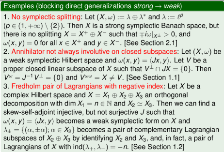
Figure 0.3. Three counterexamples

Limited value of our previous pilot study

Anyway, our previous Booß–Bavnbek, B.Zhu, C.[25] deals with a continuous family of Continuously varying!weak symplectic formsweak symplectic forms $\omega(s)$ on a curve of Continuously varying!Banach spacesBanach spaces $X(s)$, $s\in[0,1]$. It gives a definition of the Maslov indexMaslov index for a path $(\lambda(s),\mu(s))_{s\in[0,1]}$ of Fredholm pairs of Lagrangian subspaces of index $0$ under the assumption of a Continuously varying!symplectic splittingscontinuously varying symplectic splitting $X=X^{+}(s)\oplus X^{-}(s)$. The definition is inspired by the careful distinctions of planar intersections in Long, Y.Zhu, C.[108, 105, 106, 107]. Then it is shown that all nice properties of the Maslov index are preserved for this general case. However, that approach has four serious Obstructions to straight forward generalizationdrawbacks which render this definition incalculable:

1. Symplectic splittingAnnihilator!double

2. In Section 2.1, our Example 2.1.2 provides a strong symplectic Banach space that does not admit a symplectic splitting.

3. Even when a single Symplectic splitting!continuously varyingsymplectic splitting is guaranteed, there is no way to establish such splitting for families in a continuous way (see also our obstruction III above).

4. The Maslov index, as defined in [25] becomes independent of the choice of the splitting only for strong symplectic forms.

5. That construction admits finite-dimensional Symplectic reductionsymplectic reduction only for strong symplectic forms.

To us, our Booß–Bavnbek, B.Zhu, C.[25] is a highly valuable pilot study, but the preceding limitations explain why in this Memoir we begin again from scratch. For that purpose, an encouraging result was obtained in Booß–Bavnbek, B.Zhu, C.[21] combined with Chen, G.[15]: the continuous variation of the Calderón projectionCalderón projection in $L^{2}(\Sigma)$ for a Continuously varying!elliptic differential operatorscurve of elliptic differential operators of first order. We shall use this result in our Section 4.5.

Acknowledgements

We thank Prof. K. Furutani (Tokyo), Prof. M. Lesch (Bonn), and Prof. R. Nest (Copenhagen) for inspiring discussions about this subject. Last but not least, we would like to thank the referees of this paper for their critical reading and very helpful comments and suggestions. The second author was partially supported by NSFC (No.11221091 and No. 11471169), LPMC of MOE of China.

Part I Maslov index in symplectic Banach spaces

Chapter 1 General theory of symplectic analysis in Banach spaces

We fix the notation and establish our key technical device in Proposition 1.3.3 and Corollary 1.3.4, namely a natural decomposition of a fixed symplectic vector space into two symplectic subspaces induced by a single Fredholm pair of Lagrangians of index $0$. Reversing the order of the Fredholm pair, we obtain an alternative symplectic reduction. We establish the transitivity of symplectic reductions in Lemma 1.4.3 and Corollary 1.4.4. In Proposition 1.4.10, we show that the two natural symplectic reductions coincide by establishing Lemma 1.4.6. As we shall see later in Section 3, that yields the symplectic reduction to finite dimensions for a given path of Fredholm pairs of Lagrangian subspaces of index 0 in a fixed Banach space with varying symplectic structures and the invariance of the Maslov index under different symplectic reductions.

Our assumption of vanishing index is trivially satisfied in strong symplectic Hilbert space. More interestingly and inspired by and partly reformulating previous work by Schmid, R.R. Schmid, Bambusi, D.and D. Bambusi [86, 9], we obtain in Lemma 1.1.4 a delicate condition for making the annihilator an involution. In Corollary 1.2.9 we show that the index of a Fredholm pair of Lagrangian subspaces can not be positive. In Corollary 1.2.12 we derive a necessary and sufficient condition for its vanishing for weak symplectic forms and in the concrete set-up of our global analysis applications in Section 4. In order to emphasize the intricacies of weak symplectic analysis, it seems worthwhile to clarify in Lemma 1.1.4 a potentially misleading formulation in Schmid, R.[86, Lemma 7.1], and in Remark 1.2.2, to isolate an unrepairable error in Bambusi, D.[9, First claim of Lemma 3.2, pp.3387-3388], namely the wrong claim that the double annihilator is the identity on all closed subspaces of reflexive weak symplectic Banach spaces.

To settle some of the ambiguities around weak symplectic forms once and for all, we provide two counterexamples in Examples 1.2.3 and 1.2.11. The first gives a closed subspace where the double annihilator is not itself. The second gives a Fredholm pair of Lagrangians with negative index.

1.1. Dual pairs and double annihilators

Our point of departure is recognizing the difficulties of dealing with both varying and weak symplectic structures, as explained in our Booß–Bavnbek, B.Zhu, C.[25]. As shown there, a direct way to define the Maslov index in that context requires a Continuously varying!symplectic splittingscontinuously varying symplectic splitting. As mentioned in the Introduction, neither the existence nor a continuous variation of such a splitting is guaranteed. Consequently, that definition is not very helpful for calculations in applications.

To establish an intrinsic alternative, we shall postpone the use of the symplectic structures to later sections and do as much as possible in the rather neutral category of linear algebra. A first taste of the use of purely algebraic arguments of linear algebra for settling open questions of symplectic geometry is the making of a kind of Annihilator!pair annihilator of linear algebraannihilator. For the true annihilator concept of symplectic geometry see below Definition 1.2.1.c.

Already here we can explain the need for technical innovations when dealing with weak symplectic structures instead of hard ones. To give a simple example, let us consider a complex symplectic Hilbert space $(X,\langle,\rangle,\omega)$ with $w(x,y)=\langle Jx,y\rangle$ for all $x,y\in X$ where $J\colon X\to X$ is a bounded, injective and skew-self-adjoint operator (for details see below Section 1.2). Then we get at once $\lambda^{\omega}=(J\lambda)^{\bot}$ and $\lambda^{\omega\omega}\supset\overline{\lambda}$ for all linear subspaces $\lambda\subset X$. We denote the orthogonal complement by the common orthogonality exponent $\bot$ and the symplectic annihilator by the exponent $\omega$. Now, if we are in the strong symplectic case, we have $J$ surjective and $J^{2}=-I$, possibly after a slight deformation of the inner product. In that case, we have immediately

$$\lambda^{\omega\omega}=\bigl{(}J\left((J\lambda)^{\bot}\right)\bigr{)}^{\bot}=(\lambda^{\bot})^{\bot}=\overline{\lambda}.$$

Hence the double annihilator is the identity on the set of closed subspaces in strong symplectic Hilbert space, like in the familiar case of finite-dimensional symplectic analysis. Moreover, from that it follows directly that the index of a Fredholm pair of Lagrangians (see Definition 1.2.7 and Corollaries 1.2.9 and 1.2.12) vanishes in strong symplectic Hilbert space.

The preceding chain of arguments breaks down for the double annihilator in weak symplectic analysis, and we are left with two basic technical problems:

1. when do we have precisely $\lambda^{\omega\omega}=\overline{\lambda}$, and consequently,

2. when are we guaranteed the vanishing of the index of a Fredholm pair of Lagrangian subspaces?

As mentioned above, we are not the first who try to determine the precise conditions for the annihilator of an annihilator not to become larger than the closure of the original space. We are indebted to the previous work by Schmid, R.R. Schmid [86, Arguments of the proof of Lemma 7.1] and Bambusi, D.D. Bambusi [9, Arguments around Lemmata 2.7 and 3.2]. They suggested to apply a wider setting and address the Annihilator!pair annihilator of linear algebrapair-annihilator concept of linear algebra. We shall follow - and modify - some of their arguments and claims.

Definition 1.1.1.

Let $X$, $Y$ be two complex vector spaces. Denote by ${\mathbb{R}}$, ${\mathbb{C}}$ and ${\mathbb{Z}}$ the sets of real numbers, complex numbers and integers, respectively. Let $h\colon{\mathbb{C}}\to{\mathbb{C}}$ be a ${\mathbb{R}}$-linear isomorphism. Let Ω@$\Omega:X\times Y\to{\mathbb{C}}$ generalized ${\mathbb{R}}$-linear form on pair of complex vector spaces$\Omega\colon X\times Y\to{\mathbb{C}}$ be a ${\mathbb{R}}$-linear map with $\Omega(ax,by)=ah(b)\Omega(ax,by)$ for all $a,b\in{\mathbb{C}}$ and $(x,y)\in X\times Y$.
(a) For each of the subspaces $\lambda\subset X$ and $\mu\subset Y$, we define the right and left annihilators of $\lambda$ and $\mu$ as real linear subspaces of $X$ and $Y$ by

(1.1) $${\lambda@$\lambda^{\Omega,r},\mu^{\Omega,l}$rightandleftannihilatorsofsubspacesincomponentsofapairofcomplexvectorspaceswithgeneralizedbilinearform}{Annihilator!leftandright}\lambda^{\Omega,r}\ : =\ \{y\in Y;\Omega(x,y)=0,\forall x\in\lambda\},$$

(1.2) $$\mu^{\Omega,l}\ : =\ \{x\in X;\Omega(x,y)=0,\forall y\in\mu\}.$$

(b) The form $\Omega$ is said to be non-degenerate in $X$ (in $Y$) if $X^{\Omega,r}=\{0\}$ ($Y^{\Omega,l}=\{0\}$). The form $\Omega$ is said to be just non-degenerate if $X^{\Omega,r}=\{0\}$ and $Y^{\Omega,l}=\{0\}$. In that case one says that $X,Y$ form an algebraic ${\mathbb{R}}$-dual pair (see also Pedersen, G.K.Pedersen [78, 2.3.8]).
(c) We have the reduced formΩa@$\tilde{\Omega}$ induced non-degenerate reduced form for pairs of vector spaces

$$\widetilde{\Omega}\colon X/Y^{\Omega,l}\times Y/X^{\Omega,r}\longrightarrow{\mathbb{C}}$$

defined by $\widetilde{\Omega}(x+Y^{\Omega,l},y+X^{\Omega,r}):=\Omega(x,y)$ for each $(x,y)\in X\times Y$.
(d) The Ωb@$\Omega^{b}$ annihilator mapAnnihilator!annihilator mapannihilator map $\Omega^{b}\colon Y\to\operatorname{Hom}(X,{\mathbb{C}})$ is the ${\mathbb{R}}$-linear map defined by $\Omega^{b}(y)(x):=\Omega(x,y)$ for all $x\in X$.

Note​​ .

By definition, the reduced form $\widetilde{\Omega}$ is always non-degenerate, since

$$(X /Y^{\Omega,l})^{\widetilde{\Omega},r}$$

$$=\ \{y+X^{\Omega,r}\,;\,\widetilde{\Omega}\left(x+Y^{\Omega,l},y+X^{\Omega,r}\right)=\Omega(x,y)=0\,\,\forall x\in X\}$$

$$=\ X^{\Omega,r}\ =\ \{0\}\quad\text{ in $Y/X^{\Omega,r}$,}$$

making the form $\widetilde{\Omega}$ non-degenerate in $X/Y^{\Omega,l}$. Similarly, we obtain $\left(Y/X^{\Omega,r}\right)^{\widetilde{\Omega},l}=Y^{\Omega,l}$, making the form $\widetilde{\Omega}$ non-degenerate in $Y/X^{\Omega,r}$.

We list a few immediate consequences. First of all, we have $\ker_{{\mathbb{R}}}\Omega^{b}=X^{\Omega,r}$, as real vector spaces. Then we have $\lambda+Y^{\Omega,l}\subset(\lambda^{\Omega,r})^{\Omega,l}$, and $\lambda_{1}^{\Omega,r}\supset\lambda_{2}^{\Omega,r}$ if $\lambda_{1}\subset\lambda_{2}\subset X$. From that we get $\lambda^{\Omega,r}\supset((\lambda^{\Omega,r})^{\Omega,l})^{\Omega,r}\supset\lambda^{\Omega,r}$, hence

(1.3) $$\lambda^{\Omega,r}=((\lambda^{\Omega,r})^{\Omega,l})^{\Omega,r}.$$

The following lemma generalizes our Booß–Bavnbek, B.Zhu, C.[25, Lemma 5, Corollary 1]. We shall use it below in the proof of Lemma 1.2.8 to establish the general result that the index of Fredholm pairs of Lagrangians in symplectic Banach space always is non-positive. The results also hold for the bilinear forms on vector spaces over a field.

Lemma 1.1.2.

(a) If $\dim X/Y^{\Omega,l}<+\infty$, we have

$$\dim Y/X^{\Omega,r}\ =\ \dim X/Y^{\Omega,l}.$$

(b) Let $\lambda\subset\mu\subset X$ be two linear subspaces. If $\dim\mu/((\lambda^{\Omega,r})^{\Omega,l}\cap\mu)<+\infty$, we have

$$\dim\lambda^{\Omega,r}/\mu^{\Omega,r}\ =\mu/((\lambda^{\Omega,r})^{\Omega,l}\cap\mu)\leq\ \dim\mu/(\lambda+Y^{\Omega,l}\cap\mu).$$

The equality holds if and only if $(\lambda^{\Omega,r})^{\Omega,l}\cap\mu=\lambda+Y^{\Omega,l}\cap\mu$.

(c) Let $\lambda\subset X$ be a linear subspace. If $\dim(\lambda+Y^{\Omega,l})/Y^{\Omega,l}<+\infty$, we have

$$\dim(\lambda+Y^{\Omega,l})/Y^{\Omega,l}\ =\ \dim Y/\lambda^{\Omega,r}\ \mbox{\ \rm and }\ \lambda+Y^{\Omega,l}\ =\ (\lambda^{\Omega,r})^{\Omega,l}.$$

Proof.

(a) If $\dim X<+\infty$ and $X^{\Omega,r}=\{0\}$, $\Omega^{b}$ is injective. Then we have $2\dim Y=\dim_{{\mathbb{R}}}Y\leq\dim_{{\mathbb{R}}}\operatorname{Hom}(X,{\mathbb{C}})=2\dim X$. So we have $\dim Y\leq\dim X$.

If $\Omega$ is non-degenerate, we have $\dim X\leq\dim Y$ and $\dim X=\dim Y$. Applying the argument for $\widetilde{\Omega}$, we have $\dim X/Y^{\Omega,l}=\dim Y/X^{\Omega,r}$.
(b) Let $f=\Omega|_{\mu\times\lambda^{\Omega,r}}$. Then we have

$$(\mu)^{f,r}\ =\ \mu^{\Omega,r}\cap\lambda^{\Omega,r}=\mu^{\Omega,r}\text{ and }(\lambda^{\Omega,r})^{f,l}\ =\ (\lambda^{\Omega,r})^{\Omega,l}\cap\mu.$$

Note that $(\lambda^{\Omega,r})^{\Omega,l}\cap\mu\supset\lambda+Y^{\Omega,l}\cap\mu$. By (a), we get our results.
(c) Note that $(Y^{\Omega,l})^{\Omega,r}=Y$ and $(\lambda+Y^{\Omega,l})^{\Omega,r}=\lambda^{\Omega,r}\cap Y=\lambda^{\Omega,r}$. By (b) we have

$$\dim(\lambda+Y^{\Omega,l})/Y^{\Omega,l}\ =\ \dim Y/\lambda^{\Omega,r}\ \geq\ \dim(\lambda^{\Omega,r})^{\Omega,l}/Y^{\Omega,l}.$$

Since $\lambda+Y^{\Omega,l}\subset(\lambda^{\Omega,r})^{\Omega,l}$, we have $\lambda+Y^{\Omega,l}=(\lambda^{\Omega,r})^{\Omega,l}$. ∎

Assume that $\Omega$ is non-degenerate in $Y$. Then the F@${\mathcal{F}}$ family of semi-norms on first factor of paired vector spaces py@$p_{y}(\cdot)$ family of semi-norms family of semi-norms ${\mathcal{F}}:=\{p_{y}(x):=|\Omega(x,y)|,\,x\in X\}_{y\in Y}$ is separating, i.e., for $x\neq x^{\prime}$ in $X$, there is a $y\in Y$ such that $p_{y}(x-x^{\prime})\neq 0$. We shall denote the topology on $X$ induced by the family ${\mathcal{F}}$ by TT@${\mathcal{T}}_{\Omega}$ weak topology induced by pairing $\Omega$ ($\Omega$-topology) ${\mathcal{T}}_{\Omega}$ and call it the weak topology induced by $\Omega$ or shortly the $\Omega$-topology. By Pedersen, G.K.—bind[78, 1.5.3 and 3.4.2] $(X,{\mathcal{T}}_{\Omega})$ becomes a Hausdorff separated, locally convex, topological vector space. The following two lemmata are proved implicitly by Schmid, R.[86, Arguments of the proof of Lemma 7.1]. Clearly, we have

Lemma 1.1.3.

Assume that $\Omega$ is non-degenerate in $Y$. Then the real linear map $\Omega^{b}$ maps $Y$ onto $(X,{\mathcal{T}}_{\Omega})^{*}$.

Then the Hahn-Banach Extension TheoremHahn-Banach Theorem yields

Lemma 1.1.4 (R. Schmid, 1987).

Schmid’s Lemma Assume that $\Omega$ is non-degenerate in $Y$ and $\lambda$ is a closed linear subspace of $(X,{\mathcal{T}}_{\Omega})$. Then we have

(1.4) $${Annihilator!doubleannihilatoroflinearalgebra}\lambda=(\lambda^{\Omega,r})^{\Omega,l}.$$

For later use it is worth noting the following extension of Schmid’s Lemma which is the weak and corrected version of [9, Lemma 3.2].

Lemma 1.1.5.

Schmid’s Lemma Assume that $X,Y,\Omega$ as above and $\Omega$ non-degenerate in $Y$ and bounded in $X$. Assume that $X$ is a reflexive Banach space. Then $\Omega^{b}(Y)$ is dense in $X^{*}$ and we have

(1.5) $$\lambda=(\lambda^{\Omega,r})^{\Omega,l}\quad\text{for any linear and ${\mathcal{T}}_{\Omega}$-closed subspace $\lambda\subset X$}.$$

1.2. Basic symplectic concepts

Before defining the Maslov index in symplectic Banach space by symplectic reduction to the finite-dimensional case, we recall the basic concepts and properties of symplectic functional analysis.

Definition 1.2.1.

Let $X$ be a complex vector space.
(a) A mapping

$${\omega@\omega:X\times X\longrightarrow{\mathbb{C}}symplecticform}{Symplecticform!weak}\omega\colon X\times X\longrightarrow{\mathbb{C}}$$

is called a symplectic form on $X$, if it is sesquilinear, skew-symmetric, and non-degenerate, i.e.,

1. $\omega(x,y)$ is linear in $x$ and conjugate linear in $y$;

2. $\omega(y,x)\ =\ -\overline{\omega(x,y)}$;

3. $X^{\omega}\ :=\ \{x\in X;\omega(x,y)\ =\ 0\text{ for all $y\in X$}\}\ =\ \{0\}$.

Then we call $(X,\omega)$ a symplectic vector space.Symplectic structures!symplectic vector space
(b) Let $X$ be a complex Banach space and $(X,\omega)$ a symplectic vector space. $(X,\omega)$ is called (weak) symplectic Banach space, if $\omega$ is bounded, i.e., $|\omega(x,y)|\leq C\|x\|\|y\|$ for all $x,y\in X$.Symplectic structures!symplectic Banach space
(c) The annihilator of a subspace ${\lambda}$ of $X$ is defined by

$${Annihilator}{\lambda}^{\omega}\ :=\ \{y\in X;\omega(x,y)\ =\ 0\quad\text{ for all $x\in{\lambda}$}\}.$$

(d) A subspace ${\lambda}$ is called Symplectic subspacessymplectic, Isotropic subspaces isotropic, Co-isotropic subspacesco-isotropic, or Lagrangian subspacesLagrangian if

$$\lambda\cap{\lambda}^{\omega}\ =\ \{0\}\,,\quad{\lambda}\,\subset\,{\lambda}^{\omega}\,,\quad{\lambda}\,\supset\,{\lambda}^{\omega}\,,\quad{\lambda}\,\ =\ \,{\lambda}^{\omega}\,,$$

respectively.
(e) Lagrangian GrassmannianThe Lagrangian Grassmannian L@${\mathcal{L}}(X,\omega)$ Lagrangian Grassmannian${\mathcal{L}}(X,\omega)$ consists of all Lagrangian subspaces of $(X,\omega)$. We write ${\mathcal{L}}(X):={\mathcal{L}}(X,\omega)$ if there is no confusion.

Remark 1.2.2.

(a) Let $(X,\omega)$ be a complex weak symplectic Banach space. By definition (see below), the form $\omega\colon X\times X\to{\mathbb{C}}$ is non-degenerate. Then we have Topologies on symplectic Banach spaces (norm, weak, $\omega$-weak)three topologies on $X$: the norm-topology, the canonical weak topology induced from the family $X^{*}$ of continuous functionals on $X$, and the $\omega$-induced weak topology ${\mathcal{T}}_{\omega}$. The weak topology is weaker than the norm topology; and the $\omega$-induced topology is weaker than the weak topology. So, a closed subset $V\subset X$ is not necessarily weakly closed or closed in $(X,{\mathcal{T}}_{\omega})$: the set $V$ can have more accumulation points in the weak topology and even more in the $\omega$-induced weak topology than in the norm topology. A standard example is the unit sphere that is not weakly closed in infinite dimensions (see, e.g., Brezis, H.H. Brezis [27, Example 1, p. 59]. Fortunately, by [27, Theorem 3.7] every norm-closed linear subspace is weakly closed. Hence it is natural (but erroneous) to suppose that the difference between the three topologies does not necessarily confine severely the applicability of Schmid’s Lemma, namely to linear subspaces.

(b) It seems that Bambusi, D.D. Bambusi in [9, Lemmata 2.7,3.2] supposed erroneously that in reflexive Banach space all norm-closed subspaces are not only weakly closed but also $\omega$-weakly closed. Rightly, in spaces where that is valid, Schmid’s Lemma is applicable (or can be reproved independently).

(c) Recall that a Banach space $X$ is reflexive if the isometry

$$\iota\colon X\longrightarrow X^{**},\text{ given by $\iota(x)(\varphi):=\varphi(x)$ for $x\in X,\ \varphi\in X^{*}$}$$

is surjective, i.e., its range is the whole bidual space $X^{**}$. Typical examples of reflexive spaces are all Hilbert spaces and the $L^{p}$-spaces for $1<p<\infty$, but not $L^{1}$.

(d) Unfortunately, in general the claim of [9, Lemma 3.2] (the validity of the idempotence of the double annihilator for closed linear subspaces in complex reflexive symplectic Banach space) is not correct. Obstructions to straight forward generalization!double annihilator not the identity on closed subspacesIf it was correct, then, e.g., in (automatically reflexive) weak symplectic Hilbert space $(X,\langle\cdot,\cdot\rangle,\omega)$, the double annihilator $\lambda^{\omega\omega}$ of every closed subspace $\lambda$ should coincide with $\lambda$. However, here is a counterexample: Let $\left(X,\langle\cdot,\cdot\rangle\right)$ be a complex Hilbert space and $J\colon X\to X$ a bounded injective skew-self-adjoint operator. Then $\omega\colon X\times X\to{\mathbb{C}}$ defined by $\omega(x,y):=\langle Jx,y\rangle$ is a symplectic form on $X$. So $\operatorname{im}J$ is dense in $X$. For $V\subset X$ closed subspace, denote by $V^{\perp}$ the orthogonal complement of $V$ with respect to the inner product on $X$, and by λ2@$\lambda^{\omega}$ symplectic complement (annihilator) of subspace $\lambda$$V^{\omega}$ the symplectic complement (i.e., the annihilator) of $V$. Then we have

(1.6) $$V^{\omega}\ =\ (JV)^{\perp}\ =\ J^{-1}\left(V^{\perp}\right).$$

Now assume that $\operatorname{im}J\neq X$ (like in the weak symplectic Sobolev space $X:=H^{1/2}(\Sigma;E|_{\Sigma})$, as explained in the Introduction). Let $x\in X\setminus\operatorname{im}J$ and set $V:=\left(\operatorname{span}\{x\}\right)^{\perp}$. Then we have $J^{-1}\left(V^{\perp}\right)=\{0\}$, hence $V^{\omega}=\{0\}$ and $V^{\omega\omega}=X\neq V$. That contradicts the first part of Equation (13) in [9, Lemma 3.2].

(e) The preceding example contradicts [9, Equation (11)], as well: For any closed subspace $V\subset X$ we have $J\left((JV)^{\perp}\right)\subset V^{\perp}$. Then Bambusi’s Equation (11) is equivalent to

$$\overline{J\left((JV)^{\perp}\right)}\ =\ V^{\perp}.$$

For our concrete example $V:=\left(\operatorname{span}\{x\}\right)^{\perp}$, however, we obtain

$$J\left((JV)^{\perp}\right)\cap V^{\perp}=\{0\}\ \mbox{\ \rm and }\ V^{\perp}=\operatorname{span}\{x\}.$$

Thus [9, Equation (11)] is incorrect.

(f) For any Lagrangian subspace $\lambda$ in a complex symplectic Banach space $(X,\omega)$ we have $\lambda^{\omega\omega}=\lambda$ by definition. That follows also directly from the identity (1.3), and, alternatively, from Schmid’s Lemma, since a Lagrangian subspace is always $\omega$-closed.

The counterexample of the preceding Remarks d and e can be generalized in the following form.

Example 1.2.3 (Closed subspaces different from their double annihilators).

Obstructions to straight forward generalization!double annihilator not the identity on closed subspacesCounterexamples!double annihilator not the identity on closed subspaces Symplectic structures!symplectic Hilbert space Let $(X,\omega)$ be a Hilbert space!weak symplecticweak symplectic Hilbert space and $\omega(x,y)=\langle Jx,y\rangle$. Let $V$ be a proper closed linear subspace of $X$ such that $V^{\bot}\cap JX=\{0\}$. Then $V^{\omega}=J^{-1}V^{\bot}=\{0\}$ and $V^{\omega\omega}=X\supsetneqq V$.

Remark 1.2.4.

(a) By definition, each one-dimensional subspace in real symplectic space is isotropic, and there always exists a Lagrangian subspace in finite-dimensional real symplectic Banach space, namely the maximal isotropic subspace. However, there are complex symplectic Hilbert spaces Counterexamples!no Lagrangian subspacewithout any Lagrangian subspace. That is, in particular, the case if $\dim X^{+}\neq\dim X^{-}$ in ${\mathbb{N}}\cup\{\infty\}$ for a single (and hence for all) symplectic splittings. More generally, we refer to A. Weinstein’s TheoremWeinstein’s Theorem Weinstein, A.[99](see also Swanson, R.C.R.C. Swanson, [94, Theorem 2.1 and Corollary]) that relates the existence of complemented Lagrangian subspaces to the generalized Darboux, J.G.Darboux propertyDarboux property, recalled below at the end of Subsection 4.2.2.

(b) As in the finite-dimensional case, the basic geometric concept in infinite-dimensional symplectic analysis is the Lagrangian subspace, i.e., a linear subspace which is isotropic and co-isotropic at the same time. Contrary to the finite-dimensional case, however, the common definition of a Lagrangian as a maximal isotropic space or an isotropic space of half dimension becomes inappropriate.

(c) In symplectic Banach spaces, the annihilator ${\lambda}^{\omega}$ is closed for any linear subspace $\lambda$, and we have the trivial inclusion

(1.7) $${Annihilator!doubleannihilatorinsymplecticBanachspaces}{\lambda}^{\omega\omega}\supset\overline{\lambda}.$$

In particular, all Lagrangian subspaces are closed, and trivially, as emphasized in Remark 1.2.2.f, we have an equality in the preceding (1.7).

If $X$ is a complex Banach space, each symplectic form $\omega$ induces a uniquely defined mapping $J\colon X\to X^{\operatorname{ad}}$ such thatJ@$J$ operator associated to symplectic form

(1.8) $$\omega(x,y)\ =\ (Jx,y)\quad\text{ for all $x,y\in X$},$$

where we set $(Jx,y):=(Jx)(y)$. The induced mapping $J$ is a bounded, injective mapping $J\colon X\to X^{\operatorname{ad}}$ where X@$X^{\operatorname{ad}}$ space of all continuous complex-conjugate functionals on $X$$X^{\operatorname{ad}}$ denotes the (topological) dual space of continuous complex-conjugate linear functionals on $X$.

Definition 1.2.5.

Let $(X,\omega)$ be a symplectic Banach space. If $J$ is also surjective (hence with bounded inverse), the pair $(X,\omega)$ is called a strong symplectic Banach space.Symplectic form!strong

Lemma 1.2.6.

Let $(X,\omega)$ be a strong symplectic Banach space, and $\lambda\subset X$ be a linear subspace. Then we have $\lambda^{\omega\omega}=\overline{\lambda}$.

Proof.

Since $(X,\omega)$ be a strong symplectic Banach space, $J$ is surjective. So the weak topology of $X$ is the same as the $\omega$-induced weak topology. By [57, Problem III.1.34], $\overline{\lambda}$ is weakly closed. So it is also $\omega$-closed. By Lemma 1.1.4, we have $\lambda^{\omega\omega}=\overline{\lambda}$. ∎

We have taken the distinction between weak and strong symplectic structures from P. Chernoff and J. Marsden Chernoff, P.R.Marsden, J.E.[35, Section 1.2, pp. 4-5]. If $X$ is a Hilbert space with symplectic form $\omega$, we identify $X$ and $X^{*}$. Then the induced mapping $J$ defined by $\omega(x,y)=\langle Jx,y\rangle$ is a bounded, skew-self-adjoint operator (i.e., $J^{*}=-J$) on $X$ with $\ker J=\{0\}$. As in the strong symplectic case, we then have that $\lambda\subset X$ is Lagrangian if and only if $\lambda^{\perp}=J\lambda$ . As explained above, in Hilbert space, a main difference between weak and strong is that we can assume $J^{2}=-I$ in the strong case (see Booß–Bavnbek, B.Zhu, C.[25, Lemma 1] for the required smooth deformation of the inner product), but not in the weak case. The importance of such an anti-involution is well-known from symplectic analysis in finite dimensions and exploited in strong symplectic Hilbert spaces, but, in general, it is lacking in weak symplectic analysis.

We recall the key concept to symplectic analysis in infinite dimensions:

Definition 1.2.7.

The space of Fredholm pairs of Lagrangian subspaces of a symplectic vector space $(X,\omega)$ is defined byFL@${\mathcal{F}}{\mathcal{L}}(X,\omega)$ Fredholm Lagrangian GrassmannianFredholm Lagrangian Grassmannian!of symplectic vector space

(1.9) $${\mathcal{F}}{\mathcal{L}}(X)\ :=\ \{(\lambda,\mu)\in{\mathcal{L}}(X)\times{\mathcal{L}}(X);\dim(\lambda\cap\mu)<+\infty\text{ and}\\ \dim X/(\lambda+\mu)<+\infty\}$$

with index@$\operatorname{index}(\lambda,\mu)$ index of Fredholm pairFredholm pair!index Index!of Fredholm pair

(1.10) $$\operatorname{index}(\lambda,\mu)\ :=\ \dim(\lambda\cap\mu)-\dim X/(\lambda+\mu).$$

For $k\in{\mathbb{Z}}$ we defineFLk@${\mathcal{F}}{\mathcal{L}}_{k}(X),{\mathcal{F}}{\mathcal{L}}(X,\mu),{\mathcal{F}}{\mathcal{L}}_{k}(X,\mu),{\mathcal{F}}{\mathcal{L}}_{0}^{k}(X,\mu)$ subspaces of the Fredholm Lagrangian Grassmannian

(1.11) $${\mathcal{F}}{\mathcal{L}}_{k}(X)\ :=\ \{(\lambda,\mu)\in{\mathcal{F}}{\mathcal{L}}(X);\operatorname{index}(\lambda,\mu)=k\}.$$

For $k\in{\mathbb{Z}}$ and $\mu\in{\mathcal{L}}(X)$ we define

(1.12) $${\mathcal{F}}{\mathcal{L}}(X,\mu): =\ \{\lambda\in{\mathcal{L}}(X);(\lambda,\mu)\in{\mathcal{F}}{\mathcal{L}}(X)\},$$

(1.13) $${\mathcal{F}}{\mathcal{L}}_{k}(X,\mu): =\ \{\lambda\in{\mathcal{L}}(X);(\lambda,\mu)\in{\mathcal{F}}{\mathcal{L}}_{k}(X)\},$$

(1.14) $${\mathcal{F}}{\mathcal{L}}_{0}^{k}(X,\mu): =\ \{\lambda\in{\mathcal{F}}{\mathcal{L}}_{0}(X,\mu);\dim(\lambda\cap\mu)=k\}.$$

What do we know about the index of Fredholm pairs of Lagrangian subspaces in the weak symplectic case? Here we give another proof for the fact (proved before in our [25, Proposition 1]) that Fredholm pairs of Lagrangian subspaces in symplectic vector spaces never can have positive index.

Lemma 1.2.8.

Let $(X,\omega)$ be a symplectic vector space and $\lambda_{1},\ldots,\lambda_{k}$ linear subspaces of $X$. Assume that $\dim X/(\sum_{j=1}^{k}\lambda_{j})<+\infty$. Then the following holds.
(a) We have

(1.15) $$\dim(\bigcap_{j=1}^{k}\lambda_{j}^{\omega})\leq\dim X/(\sum_{j=1}^{k}\lambda_{j}).$$

The equality holds if and only if $\sum_{j=1}^{k}\lambda_{j}=(\sum_{j=1}^{k}\lambda_{j})^{\omega\omega}$.
(b) If $\lambda_{j}$ is isotropic for each $j$, we have

(1.16) $$\dim(\bigcap_{j=1}^{k}\lambda_{j})\leq\dim X/(\sum_{j=1}^{k}\lambda_{j}).$$

The equality holds if and only if $\bigcap_{j=1}^{k}\lambda_{j}=\bigcap_{j=1}^{k}\lambda_{j}^{\omega}$ and $\sum_{j=1}^{k}\lambda_{j}=(\sum_{j=1}^{k}\lambda_{j})^{\omega\omega}$.

Proof.

(a) Since $\bigcap_{j=1}^{k}\lambda_{j}^{\omega}=(\sum_{j=1}^{k}\lambda_{j})^{\omega}$, our result follows from Lemma 1.1.2.b.
(b) By (a) and $\bigcap_{j=1}^{k}\lambda_{j}\subset\bigcap_{j=1}^{k}\lambda_{j}^{\omega}$. ∎

Corollary 1.2.9 (Fredholm index never positive).

a) Let $X$ be a complex vector space with symplectic form $\omega$. Then each Fredholm pair $(\lambda,\mu)$ of Lagrangian subspaces of $(X,\omega)$ has negative index or is of index $0$.

b) If $(X,\omega)$ is a strong symplectic Banach space, then we have

(1.17) $${Annihilator!doubleannihilatorinsymplecticBanachspaces}{Index!ofFredholmpair!vanishingforLgrangiansubspacesinstrongsymplecticBanachspace}V^{\omega\omega}\ =\ V\quad\text{ for each closed subspace $V\subset X$, and}$$

(1.18) $$\operatorname{index}(\lambda,\mu)\ =\ 0\quad\text{ for each $(\lambda,\mu)\in{\mathcal{F}}{\mathcal{L}}(X,\omega)$}.$$

Proof.

(a) is immediate from the Lemma. To derive (b) from the Lemma, we shall summarize a couple of Symplectic structures!symplectic Banach space!elementary identitieselementary concepts and identities about symplectic Banach spaces:

For (1.17) we recall from (1.8) that any symplectic form $\omega$ on a complex Banach space $X$ induces a uniquely defined bounded, injective mapping $J\colon X\to X^{\operatorname{ad}}$ such that $\omega(x,y)=(Jx)(y)$ for all $x,y\in X$. Here X@$X^{\operatorname{ad}}$ space of all continuous complex-conjugate functionals on $X$$X^{\operatorname{ad}}$ denotes the space B@${\mathcal{B}}^{\operatorname{ad}}(X,Y)$ space of all continuous linear-complex-conjugate operators from $X$ to $Y$${\mathcal{B}}^{\operatorname{ad}}(X,{\mathbb{C}})$ of all continuous complex-conjugate functionals on $X$. For linear subspaces $W\subset X$ and $Z\subset X^{\operatorname{ad}}$, we set λ_bot@$\lambda^{\bot}$ dual complement of subspace $\lambda$$W^{\bot}:=\{e\in X^{\operatorname{ad}};e(x)=0\text{ for all }x\in W\}$ and $Z^{\bot}:=\{x\in X;e(x)=0\text{ for all }e\in Z\}$, as usual. By the Hahn-Banach Extension TheoremHahn-Banach extension theorem, we have

(1.19) $$W^{\bot\bot}\ =\ \overline{W}\ \mbox{\ \rm and }\ Z^{\bot\bot}\ =\ \overline{Z}.$$

Moreover, we have the following elementary identities

(1.20) $$W^{\omega}\ =\ (JW)^{\perp}\ =\ J^{-1}\left(W^{\perp}\right).$$

They correspond exactly to the identities of (1.6), given there only for $X$ symplectic Hilbert space.

Recall that we call $\omega$ strong, if $J$ is surjective, i.e., an isomorphism. That we assume now. Then we have

(1.21) $$V^{\omega\omega}\ \stackrel{{\scriptstyle i}}{{=}}\ J^{-1}(V^{\omega\bot})\ \stackrel{{\scriptstyle ii}}{{=}}\ J^{-1}((JV)^{\bot\bot})\ \stackrel{{\scriptstyle iii}}{{=}}\ J^{-1}(JV)\ \stackrel{{\scriptstyle iv}}{{=}}\ V.$$

The identities (i) and (ii) follow from (1.20) and are valid also in the weak case, while we for identity (iii) need that $J$ is bounded and surjective, hence $JV$ is closed by the Open Mapping TheoremOpen Mapping Theorem. Identity (iv) is a trivial consequence of the injectivity of $J$ and so valid also in the weak case. That proves (1.21). In particular, we have $(\lambda+\mu)^{\omega\omega}=\lambda+\mu$ and so by (b) of the Lemma $\dim(\lambda\cap\mu)=\dim X/(\lambda+\mu)$. In general, i.e., for weak symplectic form, we have $\dim(\lambda\cap\mu)=\dim X/(\lambda^{\omega}+\mu^{\omega})$ which does not suffice to prove the vanishing of the index. ∎

Remark 1.2.10.

(a) The Corollary has a wider validity. Let $(\lambda,\mu)$ be a Fredholm pair of isotropic subspaces. Then we have by Lemma 1.2.8.b $\operatorname{index}(\lambda,\mu)\leq 0$. If $\operatorname{index}(\lambda,\mu)=0$, $\lambda$ and $\mu$ are Lagrangians (see Booß–Bavnbek, B.Zhu, C.[25, Corollary 1 and Proposition 1]).
(b) To obtain $\operatorname{index}(\lambda,\mu)=0$ from Lemma 1.2.8.b for strong symplectic Banach spaces, it was crucial that we have

$$(\lambda+\mu)^{\omega\omega}=\lambda+\mu\ \mbox{\ \rm and }\ \lambda=\lambda^{\omega}\ \mbox{\ \rm and }\ \mu=\mu^{\omega}.$$

For Lagrangian subspaces the last two equations are satisfied by definition, and the first is our (1.17), valid for strong symplectic $\omega$. More generally, by Lemma 1.1.4, the first equation is satisfied if the space $\lambda+\mu$ is $\omega$-closed, i.e., closed in the weak topology ${\mathcal{T}}_{\omega}$ (see above). In a symplectic Banach space $(X,\omega)$ all Lagrangian subspaces are norm-closed, weakly closed and $\omega$-weakly closed at the same time, as emphasized in Remark 1.2.2. Since $\lambda$, $\mu$ are norm-closed and $\dim X/(\lambda+\mu)<+\infty$, $\lambda+\mu$ is norm-closed by Booß–Bavnbek, B.Furutani, K.[18, Remark A.1] and Kato, T.[58, Problem 4.4.7]. However, that does not suffice to prove that $\lambda+\mu$ is $\omega$-closed, see Remark 1.2.4.c.
(c) Our (1.18) is well known for strong symplectic Hilbert spaces (follow, e.g., the arguments of Booß–Bavnbek, B.Furutani, K.[17, Corollary 3.7]). Below, in Example 1.2.11 we give a Fredholm pair of Lagrangian subspaces in a weak symplectic Hilbert space with negative index. Hence, we can not take the vanishing of the index for granted for weak symplectic forms, neither in Hilbert spaces - contrary to the well established vanishing of the index of closed (not necessarily bounded) self-adjoint Fredholm operators in Hilbert space (Bleecker, D.Booß–Bavnbek, B.[12, p. 43]). That may appear a bit strange: Below in Section 4.2, we shall consider closed operators as special instances of Closed linear relationclosed linear relations. Then, e.g., a closed self-adjoint Fredholm operator $A$ in a Hilbert space $(X,\langle\cdot,\cdot\rangle)$ is a self-adjoint Fredholm relation, i.e., the pair $(\operatorname{graph}A,X\times\{0\})$ is a Fredholm pair of Lagrangian subspaces of the Hilbert space $X\times X$ with the canonical strong symplectic structure

(1.22) $${\omega_{c}an@\omega_{\operatorname{can}}canonicalstrongsymplecticformonX\times X^{*}}{Symplecticform!canonicalandstrongonX\times X^{*}}\omega_{\operatorname{can}}\colon(X\times X)\times(X\times X)\longrightarrow{\mathbb{C}},\quad(x_{1},y_{1},x_{2},y_{2})\mapsto\langle x_{1},y_{2}\rangle-\langle x_{2},y_{1}\rangle.$$

That yields an alternative, namely symplectic proof of the vanishing of the index of a closed self-adjoint Fredholm operator in Hilbert space, since $\operatorname{index}A=\operatorname{index}(\operatorname{graph}A,X\times\{0\})$ by (4.6) and $(\operatorname{graph}A,X\times\{0\})$ a Fredholm pair of Lagrangian subspaces of $(X\times X,\omega_{\operatorname{can}})$. The preceding arguments generalize immediately for any Fredholm operator!closed self-adjointIndex!of closed self-adjoint Fredholm operator closed self-adjoint Fredholm operator $A\colon X\to X^{*}$ with $\operatorname{dom}A\subset X$ and $X$ reflexive complex Banach space. We only need to reformulate the canonical strong symplectic form in (1.22) on the Banach space $X\times X^{*}$, replacing $X\times X$ by $X\times X^{*}$ and $\langle x,y\rangle$ by $y(x)$. That yields a strong symplectic form if and only if $X$ is reflexive. For examples of self-adjoint Fredholm operators in “non-Hilbertable” Banach space!non-HilbertableBanach spaces we refer to self-adjoint extensions of the Laplacian in $L^{p}$-spaces appearing with convex Hamiltonian system!self-adjoint extensions of the LaplacianHamiltonian systems in Ekeland, I.I. Ekeland [45, p. 108]. Later in Section 4.2.2, for our applications we shall introduce a new (and weak) concept of a Fredholm operator $A\colon X\to Y$ in Banach spaces $X,Y$ that is “self-adjoint” relative to a weak symplectic structure on $X\times Y$ induced by a non-degenerate sesquilinear form $\Omega\colon X\times Y\to{\mathbb{C}}$. A priori, we can not exclude Counterexamples!non-vanishing index for self-adjoint Fredholm operators in Banach spaces with non-degenerate sesquilinear forms.
(d) In view of our Example 1.2.11, we shall need special assumptions below in Chapter 4 to exclude intractable complications with index calculations for arbitrary Fredholm relations and “self-adjoint” Fredholm operators (e.g., see the assumptions of Proposition 4.3.1, Assumption 4.3.3 (iv), and Assumption 4.4.1 (iv)).
(e) In our applications, we shall deal only with Fredholm pairs of Lagrangians where the vanishing of the index is granted by arguments of global analysis or simply because the underlying form is strong symplectic.

Here is an example which shows that the index of a Fredholm pair of Lagrangian subspaces in weak symplectic Banach space need not vanish.

Example 1.2.11 (Fredholm pairs of Lagrangians with negative index).

Obstructions to straight forward generalization!non-vanishing index of Fredholm pair of Lagrangian subspacesHilbert space!weak symplectic Counterexamples!non-vanishing index of Fredholm pair of Lagrangian subspaces Let $X$ be a complex Hilbert space and $X=X_{1}\oplus X_{2}\oplus X_{3}$ an orthogonal decomposition with $\dim X_{1}=n\in{\mathbb{N}}$ and $X_{2}\simeq X_{3}$. Then we can find a bounded skew-self-adjoint injective, but not surjective $J\colon X\to X$ such that $\omega(x,y)=\langle Jx,y\rangle$ becomes a weak symplectic form on $X$. Let $J$ be of the form

$$J=i\left(\begin{array}[]{ccc}A_{11}&A_{12}&\bar{k}A_{12}\\ A_{21}&A_{22}&0\\ kA_{21}&0&-A_{22}\end{array}\right),$$

where $k\in{\mathbb{C}},k\neq\pm 1$, $\operatorname{im}A_{21}\cap\operatorname{im}A_{22}=\{0\}$ and $\ker A_{21}=\ker A_{22}=\{0\}$.

Set $V=X_{2}\oplus X_{3}$. We identify the vectors in $X_{2}$ and $X_{3}$. Then the pair $(\lambda_{+},\lambda_{-})$ with $\lambda_{\pm}:=\{(\alpha,\pm\alpha);\alpha\in X_{2}\}$ becomes a Fredholm pair of Lagrangian subspaces of $(V,\omega|_{V})$ with $\lambda_{+}\cap\lambda_{-}=\{0\}$ and

$$V\ =\ \lambda_{+}\oplus\lambda_{-}.$$

We claim that $J^{-1}(X_{1}\oplus\lambda_{\pm})\subset V$. In fact, let $(x_{1},x_{2},x_{3})\in J^{-1}(X_{1}\oplus\lambda_{\pm})$. Then there is an $\alpha\in X_{2}$ such that $A_{21}x_{1}+A_{22}x_{2}=\alpha$ and $kA_{21}x_{1}-A_{22}x_{3}=\pm\alpha$. So $(1\mp k)A_{21}x_{1}+A_{22}(x_{2}\pm x_{3})=0$. Since $\operatorname{im}A_{21}\cap\operatorname{im}A_{22}=0$ and $\ker A_{21}=0$, we have $x_{1}=0$.

Note that $\lambda_{\pm}^{\bot}=X_{1}\oplus\lambda_{\mp}$ and $\lambda_{\pm}^{\omega}\cap V=\lambda^{\pm}$. Then we have $\lambda_{\pm}^{\omega}=J^{-1}(X_{1}\oplus\lambda_{\mp})\subset V$ and $\lambda_{\pm}^{\omega}=\lambda_{\pm}^{\omega}\cap V=\lambda^{\pm}$. So $\lambda_{\pm}$ are Lagrangian subspaces of $(X,\omega)$. Then, by definition of $J$ they form a Fredholm pair of Lagrangians of $X$ with $\operatorname{index}(\lambda_{+},\lambda_{-})=-n$.

Corollary 1.2.12.

Let $(X,\omega)$ be a symplectic vector space and $\lambda,\mu$ two linear subspaces. Assume that

$$\dim X/(\lambda+\mu)<+\infty\text{ and }\dim X/(\lambda^{\omega}+\mu^{\omega})<+\infty.$$

Then the following holds.
(a) $(\lambda,\mu)$ and $(\lambda^{\omega},\mu^{\omega})$ are Fredholm pairs, and we have

(1.24) $$\operatorname{index}(\lambda,\mu)\ +\ \operatorname{index}(\lambda^{\omega},\mu^{\omega})\ \leq\ 0.$$

(b) The equality holds in (1.24) if and only if $\lambda+\mu=(\lambda+\mu)^{\omega\omega}$, $\lambda^{\omega}+\mu^{\omega}=(\lambda^{\omega}+\mu^{\omega})^{\omega\omega}$, and $\lambda\cap\mu=\lambda^{\omega\omega}\cap\mu^{\omega\omega}$.

Proof.

(a) By Lemma 1.2.8, we have

(1.25) $$\dim(\lambda^{\omega}\cap\mu^{\omega})\leq\dim X/(\lambda+\mu)<+\infty,$$

(1.26) $$\dim(\lambda\cap\mu)\leq\dim(\lambda^{\omega\omega}\cap\mu^{\omega\omega})\leq\dim X/(\lambda^{\omega}+\mu^{\omega})<+\infty.$$

Then $(\lambda,\mu)$ and $(\lambda^{\omega},\mu^{\omega})$ are Fredholm pairs, and we have

$$\operatorname{index}(\lambda,\mu)+\operatorname{index}(\lambda^{\omega},\mu^{\omega})\ =\ \dim(\lambda\cap\mu)-\dim X/(\lambda+\mu)$$

$$\qquad+\dim(\lambda^{\omega}\cap\mu^{\omega})-\dim X/(\lambda^{\omega}+\mu^{\omega})$$

$$=\ \dim(\lambda\cap\mu)-\dim X/(\lambda^{\omega}+\mu^{\omega})$$

$$\qquad+\dim(\lambda^{\omega}\cap\mu^{\omega})-\dim X/(\lambda+\mu)\leq 0.$$

(b) By the proof of (a), the equality in (1.24) holds if and only if $\dim(\lambda^{\omega}\cap\mu^{\omega})=\dim X/(\lambda+\mu)$ and $\dim(\lambda\cap\mu)=\dim(\lambda^{\omega\omega}\cap\mu^{\omega\omega})=\dim X/(\lambda^{\omega}+\mu^{\omega})$. Since $\lambda\cap\mu\subset\lambda^{\omega\omega}\cap\mu^{\omega\omega}$, by Lemma 1.2.8, the equality in (1.24) holds if and only if $\lambda+\mu=(\lambda+\mu)^{\omega\omega}$, $\lambda^{\omega}+\mu^{\omega}=(\lambda^{\omega}+\mu^{\omega})^{\omega\omega}$, and $\lambda\cap\mu=\lambda^{\omega\omega}\cap\mu^{\omega\omega}$. ∎

1.3. Natural decomposition of $X$ induced by a Fredholm pair of Lagrangian subspaces with vanishing index

The following lemmata are the key to the definition of the Maslov index in symplectic Banach spaces by symplectic reduction to the finite-dimensional case. For technical reasons, in this section, Fredholm pairs of Lagrangians are always assumed to be of index $0$.

We begin with some general facts.

Lemma 1.3.1.

Let $(X,\omega)$ be a symplectic vector space and $X_{0},X_{1}$ two linear subspaces with $X=X_{0}+X_{1}$. Assume that $X_{0}\subset X_{1}^{\omega}$. Then we have $X_{0}=X_{1}^{\omega}$, $X_{1}=X_{0}^{\omega}$, $X=X_{0}\oplus X_{1}$, and $X_{0},X_{1}$ are symplectic.

Proof.

Since $X_{0}\subset X_{1}^{\omega}$, we have $X_{1}\subset X_{1}^{\omega\omega}\subset X_{0}^{\omega}$. Since $X=X_{0}+X_{1}$, there holds

$$X_{1}\cap X_{1}^{\omega}\subset X_{0}^{\omega}\cap X_{1}^{\omega}=(X_{0}+X_{1})^{\omega}=\{0\}.$$

So $X_{1}$ is symplectic, and we have $X_{1}^{\omega}=X_{1}^{\omega}\cap(X_{0}+X_{1})=X_{0}+X_{1}^{\omega}\cap X_{1}=X_{0}$ and $X_{1}\cap X_{0}=X_{1}\cap X_{1}^{\omega}=\{0\}$. Hence we have $X=X_{0}\oplus X_{1}$. Since $X_{1}\subset X_{0}^{\omega}$ and $X=X_{0}+X_{1}$, we have $X_{1}=X_{0}^{\omega}$ and $X_{0}$ is symplectic. ∎

Lemma 1.3.2.

Let $(X,\omega)$ be a symplectic vector space and $\lambda,V$ two linear subspaces. Assume that $\dim V<+\infty$. Then we have

(1.27) $$\dim\lambda/(\lambda\cap V^{\omega})\leq\dim V.$$

The equality holds if and only if $\lambda+V^{\omega}=X$. In this case we have $\lambda^{\omega}\cap V=\{0\}$.

Proof.

By Booß–Bavnbek, B.Zhu, C.[25, Corollary 1], we have $\dim X/V^{\omega}=\dim V$. Hence we have

$$\dim\lambda/(\lambda\cap V^{\omega})=\dim(\lambda+V^{\omega})/V^{\omega}\leq\dim X/V^{\omega}=\dim V.$$

The equality holds if and only if $\lambda+V^{\omega}=X$. In this case we have $\lambda^{\omega}\cap V=(\lambda+V^{\omega})^{\omega}=\{0\}$. ∎

Now we turn to our key observation.Natural decomposition of a symplectic vector space Symplectic reduction!decomposition induced by a pair of co-isotropic subspaces

Proposition 1.3.3.

Let $(X,\omega)$ be a symplectic vector space. Let $(\lambda,\mu)$ be a pair of co-isotropic subspaces with $\dim\lambda_{0}=\dim X/(\lambda+\mu)<+\infty$, where $\lambda_{0}=\lambda^{\omega}\cap\mu^{\omega}$. Let $V$ be a linear subspace of $X$ with $X=V\oplus(\lambda+\mu)$. Let $\lambda_{1}=V^{\omega}\cap\lambda$ and $\mu_{1}=V^{\omega}\cap\mu$. Let $X_{0}=\lambda_{0}+V$ and $X_{1}=\lambda_{1}+\mu_{1}$. Then the following holds.
(a) $V^{\omega}\oplus\lambda_{0}=X$.
(b) $X_{0}=\lambda_{0}\oplus V$, $\lambda=\lambda_{0}\oplus\lambda_{1}$ and $\mu=\lambda_{0}\oplus\mu_{1}$. $X_{1}=\lambda_{1}\oplus\mu_{1}$ if $\lambda$ and $\mu$ are Lagrangian subspaces of $X$.
(c) $\lambda_{1}=\lambda\cap X_{1}$, $\mu_{1}=\mu\cap X_{1}$ and $\lambda+\mu=\lambda_{0}+X_{1}$.
(d) $X_{1}=X_{0}^{\omega}=V^{\omega}\cap(\lambda+\mu)$, $X_{0}=X_{1}^{\omega}$, $X=X_{0}\oplus X_{1}$, and $X_{0}$ and $X_{1}$ are symplectic.
(e) The subspace $\lambda_{0}$ is a Lagrangian subspace of $X_{0}$. $\lambda_{1},\mu_{1}$ are Lagrangian subspaces of $X_{1}$ if $\lambda$ and $\mu$ are Lagrangian subspaces of $X$.

Proof.

(a) Since $X=V\oplus(\lambda+\mu)$, we have $V\cap\lambda_{0}=\{0\}$ and $V^{\omega}\cap\lambda_{0}=\{0\}$. By Booß–Bavnbek, B.Zhu, C.[25, Corollary 1], we have $\dim X/V^{\omega}=\dim V=\dim\lambda_{0}$. So we have $X=V^{\omega}\oplus\lambda_{0}$.
(b) Note that

$$\dim\lambda_{0}\ \leq\ \dim\lambda/(V^{\omega}\cap\lambda)\ =\ \dim(V^{\omega}+\lambda)/V^{\omega}$$

$$\leq\ \dim X/V^{\omega}\ \leq\ \dim V\ =\ \dim\lambda_{0}.$$

We have $\lambda_{1}\cap\mu_{1}=V^{\omega}\cap\lambda\cap\mu=V^{\omega}\cap\lambda_{0}=\{0\}$ if $\lambda$ and $\mu$ are Lagrangian subspaces of $X$. So (b) holds.
(c) Since $X_{1}=\lambda_{1}+\mu_{1}\subset V^{\omega}$, we have $\lambda\cap X_{1}\subset\lambda_{1}\subset\lambda\cap X_{1}$. So $\lambda_{1}=\lambda\cap X_{1}$ holds. Similarly we have $\mu_{1}=\mu\cap X_{1}$. By (b) we have

$$\lambda+\mu=\lambda_{0}+\lambda_{1}+\lambda_{0}+\mu_{1}=\lambda_{0}+\lambda_{1}+\mu_{1}=\lambda_{0}+X_{1}.$$

(d) Since $X=X_{0}+X_{1}$, our claim follows from Lemma 1.3.1 and the fact

$$X_{0}^{\omega}=V^{\omega}\cap\lambda_{0}^{\omega}\supset V^{\omega}\cap(\lambda+\mu)\supset X_{1}.$$

(e) By definition, $\lambda_{0}$ is isotropic. Moreover, $\dim\lambda_{0}=\frac{1}{2}\dim X_{0}$. So $\lambda_{0}$ is Lagrangian in $X_{0}$.

Now assume that $\lambda$ and $\mu$ are Lagrangian subspaces of $X$. Note that $\lambda_{1}$ and $\mu_{1}$ are isotropic. Since $X_{1}=\lambda_{1}\oplus\mu_{1}$, by Booß–Bavnbek, B.Zhu, C.[25, Lemma 4], $\lambda_{1}$ and $\mu_{1}$ are Lagrangian subspaces of $X_{1}$. ∎

Corollary 1.3.4.

Let $(X,\omega)$ be a symplectic vector space. Let $(\lambda,\mu)$ be a Fredholm pair of Lagrangian subspaces of index $0$. Then there exists a Lagrangian subspace $\widetilde{\mu}\subset X$ such that $X=\lambda\oplus\widetilde{\mu}$ and $\dim\mu/(\mu\cap\widetilde{\mu})=\dim\widetilde{\mu}/(\mu\cap\widetilde{\mu})=\dim(\lambda\cap\mu)$.

Proof.

By Proposition 1.3.3, $X_{0}$ is symplectic and $\lambda_{0}$ is a Lagrangian subspace of $X_{0}$. Choose a Lagrangian $\widetilde{V}$ of $X_{0}$ with $X_{0}=\lambda_{0}\oplus\widetilde{V}$. Then set $\widetilde{\mu}:=\widetilde{V}\oplus\mu_{1}$. ∎

Lemma 1.3.5.

Let $(X,\omega)$ be a symplectic vector space and $\lambda$ an isotropic subspace of $X$. Assume that $\dim\lambda=n<+\infty$. Then there exists a $2n$ dimensional symplectic subspace $X_{0}$ such that $\lambda$ is a Lagrangian subspace of $X_{0}$, $X_{0}=X_{0}^{\omega\omega}$ and $X=X_{0}\oplus X_{0}^{\omega}$.

Proof.

Since $\dim\lambda=n<+\infty$, by Booß–Bavnbek, B.Zhu, C.[25, Corollary 1] we have $\lambda^{\omega\omega}=\lambda$ and $\dim X/\lambda^{\omega}=n$. Take an $n$ dimensional linear subspace $V$ of $X$ such that $X=V\oplus\lambda^{\omega}$. Since $\lambda\subset\lambda^{\omega}$, we have

$$\lambda^{\omega}\cap(\lambda+V)=\lambda+\lambda^{\omega}\cap V=\lambda.$$

Since $\dim V=n<+\infty$, by Booß–Bavnbek, B.Zhu, C.[25, Corollary 1] we have $V^{\omega\omega}=V$ and $\dim X/V^{\omega}=n$. Set $X_{0}:=\lambda+V$. Then we have

$$X_{0}\cap X_{0}^{\omega}=(\lambda+V)\cap\lambda^{\omega}\cap V^{\omega}=\lambda\cap V^{\omega}=(\lambda^{\omega}+V)^{\omega}=\{0\}.$$

By Booß–Bavnbek, B.Zhu, C.[25, Corollary 1], $\dim X/X_{0}^{\omega}=\dim X_{0}=2n$ and $X_{0}^{\omega\omega}=X_{0}$. So we have $X=X_{0}\oplus X_{0}^{\omega}$. Since $\dim\lambda=n$ and $\lambda$ is isotropic, $\lambda$ is a Lagrangian subspace of $X_{0}$. ∎

Lemma 1.3.6.

Let $\varepsilon$ be a positive number. Let $(X,\omega(s))$, $s\in(-\varepsilon,\varepsilon)$ be a family of symplectic Banach space with Continuously varying!symplectic formscontinuously varying $\omega(s)$. Let $X_{0}(s)$, $s\in(-\varepsilon,\varepsilon)$ be a Continuously varying!linear subspacescontinuous family of linear subspaces of dimension $2n<+\infty$ such that $(X_{0}(0),\omega(0)|_{X_{0}(0)})$ is symplectic. Let $\lambda(0)$ be a Lagrangian subspace of $(X_{0}(0),\omega(0)|_{X_{0}(0)})$. Then there exist a $\delta\in(0,\varepsilon)$ and a continuous family of linear subspaces $\lambda(s)$, $s\in(-\delta,\delta)$ such that $(X_{0}(s),\omega(s)|_{X_{0}(s)})$ is symplectic and $\lambda(s)$ is a Lagrangian subspace of $(X_{0}(s),\omega(s)|_{X_{0}(s)})$ for each $s\in(-\delta,\delta)$.

Proof.

Since $\dim X_{0}(s)=2n<+\infty$, by the proof of Kato, T.[58, Lemma III.1.40], there exists a closed subspace $X_{1}$ such that $X=X_{0}(0)\oplus X_{1}$. By Proposition A.3.5, there exists a $\delta_{1}\in(0,\varepsilon)$ such that $X=X_{0}(s)\oplus X_{1}$ for each $s\in(-\delta_{1},\delta_{1})$. By Kato, T.[58, Lemma I.4.10], there exist a $\delta_{2}\in(0,\delta_{1})$ and a continuous family $U(s)\in{\mathcal{B}}(X)$, $s\in[0,\delta_{2})$ of such that $U(s)^{-1}\in{\mathcal{B}}(X)$ and $U(s)X_{0}(0)=X_{0}(s)$.

Since $X_{0}(0)$ is symplectic, there exists a $\delta_{3}\in(0,\delta_{2})$ such that the form

$$U(s)^{*}(\omega(s)|_{X_{0}(s)})(x,y):=\omega(s)(U(s)x,U(s)y),\quad x,y\in X_{0}(0)$$

is a symplectic form on $X_{0}(0)$ for each $s\in[0,\delta_{3})$. Then the form $\omega(s)|_{X_{0}(s)}$ is symplectic.

We give $X_{0}(0)$ an inner product $\langle\cdot,\cdot\rangle$. Let $J_{0}(s)\in\operatorname{GL}(X_{0}(0))$ be the operators that define the symplectic structures $U(s)^{*}(\omega(s)|_{X_{0}(s)})$. Then there exists a continuous family $T(s)\in\operatorname{GL}(X_{0}(0))$, $s\in(-\delta,\delta)$ with $\delta\in(0,\delta_{3})$ such that $T(s)^{*}J_{0}(s)T(s)=J_{0}(0)$, where we set $\lambda(s):=U(s)T(s)\lambda(0)$ and our result follows. ∎

1.4. Symplectic reduction of Fredholm pairs

We recall the general definition of symplectic reduction.

Definition 1.4.1.

Let $(X,\omega)$ be a symplectic vector space and $W$ a co-isotropic subspace.
(a) The space $W/W^{\omega}$ is a symplectic vector space with induced symplectic structure

(1.28) $$\widetilde{\omega}(x+W^{\omega},y+W^{\omega})\ :=\ \omega(x,y)\text{ for all $x,y\in W$}.$$

We call W@$W/W^{\omega}$ reduced symplectic space ωtilde@$\tilde{\omega}$ induced form on symplectic reduction $(W/W^{\omega},\widetilde{\omega})$ the symplectic reduction of $X$ via $W$.
(b) Let $\lambda$ be a linear subspace of $X$. Symplectic reductionThe symplectic reduction of $\lambda$ via $W$ is defined by

(1.29) $${R@R_{W}(\lambda)symplecticreductionofisotropic\lambda alongco-isotropicW}{Symplecticreduction!reductionmap}R_{W}(\lambda)=R_{W}^{\omega}(\lambda)\ :=\ \bigl{(}(\lambda+W^{\omega})\cap W\bigr{)}/W^{\omega}\ =\ \bigl{(}\lambda\cap W+W^{\omega}\bigr{)}/W^{\omega}.$$

Clearly, $R_{W}(\lambda)$ is isotropic if $\lambda$ is isotropic. If $W^{\omega}\subset\lambda\subset W$ and $\lambda$ is Lagrangian, $R_{W}(\lambda)$ is Lagrangian. We have the following lemma.

Lemma 1.4.2.

Let $(X,\omega)$ be a symplectic vector space with isotropic subspace $W_{0}$. Let $\lambda\supset W_{0}$ be a linear subspace. Then $\lambda$ is a Lagrangian subspace of $X$ if and only if $W_{0}^{\omega\omega}\subset\lambda\subset W_{0}^{\omega}$ and $R_{W_{0}^{\omega}}(\lambda)$ is a Lagrangian subspace of $W_{0}^{\omega}/W_{0}^{\omega\omega}$.

Proof.

By (1.3) we have $W_{0}^{\omega\omega\omega}=W_{0}^{\omega}$. Since $W_{0}\subset W_{0}^{\omega}$, $W_{0}^{\omega\omega}\subset W_{0}^{\omega}$.

If $\lambda\in{\mathcal{L}}(X)$ and $\lambda\supset W_{0}$, we have $\lambda\subset W_{0}^{\omega}$ and $W_{0}^{\omega\omega}\subset\lambda$. Then we get $R_{W_{0}^{\omega}}(\lambda)=\lambda/W_{0}^{\omega\omega}$ and $(\lambda/W_{0}^{\omega\omega})^{\widetilde{\omega}}=(\lambda^{\omega}\cap W_{0}^{\omega})/W_{0}^{\omega\omega}=\lambda/W_{0}^{\omega\omega}$, i.e., $R_{W_{0}^{\omega}}(\lambda)\in{\mathcal{L}}(W_{0}^{\omega}/W_{0}^{\omega\omega})$.

Assume that $W_{0}^{\omega\omega}\subset\lambda\subset W_{0}^{\omega}$, we have $W_{0}^{\omega\omega}\subset\lambda^{\omega}\subset W_{0}^{\omega}$. If $R_{W_{0}^{\omega}}(\lambda)\in{\mathcal{L}}(W_{0}^{\omega}/W_{0}^{\omega\omega})$, we have

$$\lambda/W_{0}^{\omega\omega}=(\lambda/W_{0}^{\omega\omega})^{\widetilde{\omega}}=(\lambda^{\omega}\cap W_{0}^{\omega})/W_{0}^{\omega\omega}=\lambda^{\omega}/W_{0}^{\omega\omega}.$$

So we get $\lambda=\lambda^{\omega}$, i.e., $\lambda\in{\mathcal{L}}(X)$. ∎

Lemma 1.4.3 (Transitivity of symplectic reduction).

Symplectic reduction!transitivity Let $(X,\omega)$ be a symplectic vector space with two co-isotropic subspaces $W_{1}\subset W_{2}$, hence clearly $W_{1}/W_{2}^{\omega}\subset W_{2}/W_{2}^{\omega}$ with $(W_{1}/W_{2}^{\omega})^{\omega_{2}}=W_{1}^{\omega}/W_{2}^{\omega}$, where $\omega_{2}$ denotes the symplectic form on $W_{2}/W_{2}^{\omega}$ induced by $\omega$. Then the following holds.
(a) Denote by $K_{W_{1},W_{2}}\colon W_{1}/W_{2}^{\omega}\longrightarrow W_{1}/W_{1}^{\omega}$ the map induced by $I_{W_{1}}$, where $I_{W}$ denotes the identity map on a space $W$. Then $K_{W_{1},W_{2}}$ induces a symplectic isomorphism

(1.30) $$\widetilde{K}_{W_{1},W_{2}}\colon(W_{1}/W_{2}^{\omega})/(W_{1}^{\omega}/W_{2}^{\omega})\longrightarrow W_{1}/W_{1}^{\omega},$$

such that the following diagram becomes commutative:

(1.31)

(b) For a linear subspace of $\lambda$ of $X$, we have

(1.32) $$R_{W_{1}/W_{2}^{\omega}}(R_{W_{2}}(\lambda))=\widetilde{K}_{W_{1},W_{2}}^{-1}(R_{W_{1}}(\lambda)).$$

Differently put, the following diagram is commutative:

(1.33)

RW1@$R_{W_{1}/W_{2}^{\omega}}$ inner symplectic reductionSymplectic reduction!inner Here Lin@$\operatorname{Lin}(X)$ set of linear subspaces of the vector space $X$$\operatorname{Lin}(X)$ denotes the set of linear subspaces of the vector space $X$.

Proof.

(a) Since $W_{1}\subset W_{2}$ and they are co-isotropic, we have $W_{2}^{\omega}\subset W_{1}^{\omega}\subset W_{1}\subset W_{2}$. So $K_{W_{1},W_{2}}$ is well-defined. Since $\ker K_{W_{1},W_{2}}=W_{1}^{\omega}/W_{2}^{\omega}$, $\widetilde{K}_{W_{1},W_{2}}$ is a linear isomorphism. By Definition 1.4.1, $\widetilde{K}_{W_{1},W_{2}}$ is a symplectic isomorphism.

(b) Note that

$$R_{W_{2}}(\lambda)\cap(W_{1} /W_{2}^{\omega})+W_{1}^{\omega}/W_{2}^{\omega}=\bigl{(}(\lambda\cap W_{2}+W_{2}^{\omega})\cap W_{1}+W_{1}^{\omega}\bigr{)}/W_{2}^{\omega}$$

$$=(\lambda\cap W_{1}+W_{2}^{\omega}+W_{1}^{\omega})/W_{2}^{\omega}=(\lambda\cap W_{1}+W_{1}^{\omega})/W_{2}^{\omega}.$$

So (1.32) holds. ∎

Corollary 1.4.4.

Let $(X,\omega)$ be a symplectic vector space with a co-isotropic subspace $W$, a Lagrangian subspace $\mu$ and two linear spaces $V,\lambda$. Assume that $\dim W^{\omega}\cap\mu=\dim X/(W+\mu)=\dim V<+\infty$, $X=V\oplus(W+\mu)$ and $W^{\omega}\cap\mu\subset\lambda\subset W+\mu$. Set $X_{0}:=W^{\omega}\cap\mu+V$ and $X_{1}:=V^{\omega}\cap W+V^{\omega}\cap\mu$. Denote by $P_{1}\colon X\to X_{1}$ defined by $X=X_{0}\oplus X_{1}$ (see Proposition 1.3.3). Then the following holds.
(a) $W\cap X_{1}=V^{\omega}\cap W$, $W^{\omega}\cap X_{1}=W^{\omega}\cap V^{\omega}$, $\mu\cap X_{1}=V^{\omega}\cap\mu$, $\lambda=W^{\omega}\cap\mu+\lambda\cap X_{1}$, and $(W\cap X_{1})^{\omega}=W^{\omega}+V=X_{0}+W^{\omega}\cap X_{1}$.
(b) $P_{1}$ induces a symplectic isomorphism

$$\widetilde{P}_{1}\colon(W+\mu)/(W^{\omega}\cap\mu)\longrightarrow X_{1}\ \mbox{\ \rm and }\ \widetilde{P}_{1}(R_{W+\mu}(\lambda))\ =\ \lambda\cap X_{1}.$$

(c) Denote by $R^{X_{1}}_{V^{\omega}\cap W}(\lambda\cap X_{1})$ the symplectic reduction of $\lambda\cap X_{1}$ in $X_{1}$ via $V^{\omega}\cap W$. Define $\widetilde{L}_{W,W+\mu}\colon(W\cap X_{1})/(W^{\omega}\cap X_{1})\to W/W^{\omega}$ by $\widetilde{L}_{W,W+\mu}(x+W^{\omega}\cap X_{1})=x+W^{\omega}$ for all $x\in W\cap X_{1}$. Then the following diagram is commutative

(1.34)

and, in particular, we have

(1.35) $$R^{X_{1}}_{V^{\omega}\cap W}(\lambda\cap X_{1})=\widetilde{L}^{-1}_{W,W+\mu}(R_{W}(\lambda)).$$

Here $\operatorname{Lin}_{W,\mu}(X):=\{\lambda\in\operatorname{Lin}(X);W^{\omega}\cap\mu\subset\lambda\subset W+\mu\}$.
(d) $W$ is complemented (see Remark 1.4.5) in $X$ if and only if $W\cap X_{1}$ is complemented in $X_{1}$. In the case of a Banach space we require all the appeared subspaces to be closed.
(e) $W^{\omega}$ is complemented in $W$ if and only if $W^{\omega}\cap X_{1}$ is complemented in $W\cap X_{1}$. In the case of a Banach space we require all the appeared subspaces to be closed.

Proof.

(a) By Proposition 1.3.3, we have $W\cap X_{1}=V^{\omega}\cap W$, $\mu\cap X_{1}=V^{\omega}\cap\mu$, $W+\mu=W^{\omega}\cap\mu+X_{1}$, and $X=V^{\omega}+W=V^{\omega}+\mu$. Since $W+V=W+X_{0}$ and $X_{1}=X_{0}^{\omega}$, we have

$$W^{\omega}\cap V^{\omega}=(W+V)^{\omega}=(W+X_{0})^{\omega}=W^{\omega}\cap X_{1}.$$

Since $W^{\omega}\cap\mu\subset\lambda\subset W+\mu$, we have

$$\lambda=\lambda\cap(W+\mu)=\lambda\cap(W^{\omega}\cap\mu+X_{1})=W^{\omega}\cap\mu+\lambda\cap X_{1}.$$

Note that $W=W^{\omega}\cap\mu\oplus W\cap X_{1}$. By Lemma 1.1.2.b we have $\dim(W\cap X_{1})^{\omega}/W^{\omega}\leq\dim(W^{\omega}\cap\mu)=\dim V$. Moreover, we have

$$(W\cap X_{1})^{\omega}\supset W^{\omega}+X_{1}^{\omega}=W^{\omega}+X_{0}=W^{\omega}+V.$$

Since $W^{\omega}\cap V=(W+V^{\omega})^{\omega}=\{0\}$, we have

$$(W\cap X_{1})^{\omega}=W^{\omega}+V=X_{0}+W^{\omega}\cap X_{1}.$$

(b) Since $W^{\omega}\cap\mu$ is isotropic and $W+\mu=W^{\omega}\cap\mu\oplus X_{1}$, $P_{1}$ induces a symplectic isomorphism $\widetilde{P}_{1}\colon(W+\mu)/(W^{\omega}\cap\mu)\to X_{1}$. Since $W^{\omega}\cap\mu\subset\lambda\subset W+\mu$, we have $R_{W+\mu}(\lambda)=\lambda/(W^{\omega}\cap\mu)$. So it holds that $\widetilde{P}_{1}(R_{W+\mu}(\lambda))=\lambda\cap X_{1}$.

(c) Let $\widetilde{K}_{W,W+\mu}$ denote the symplectic isomorphism defined by (1.30). Note that $\widetilde{K}_{W,W+\mu}=\widetilde{L}_{W,W+\mu}$ under the symplectic isomorphism $\widetilde{P}_{1}$. So (1.35) follows from (b) and Lemma 1.4.3.

(d) If $W\cap X_{1}$ is complemented in $X_{1}$, there exists a linear subspace $M_{1}$ such that $X_{1}=W\cap X_{1}\oplus M_{1}$. Since $\dim X_{0}<+\infty$, there exists a linear subspace $M_{0}$ such that $X_{0}=W^{\omega}\cap\mu\oplus M_{0}$. Take $M=M_{0}\oplus M_{1}$ and we have $X=W\oplus M$.

Conversely, if $W$ is complemented in $X$, there exists a linear subspace of $M$ such that $X=W\oplus M$. By (a), we have $W=W\cap X_{1}\oplus W^{\omega}\cap\mu$. So we have

$$X_{1}=X_{1}\cap(W\cap X_{1}+W^{\omega}\cap\mu+M)=W\cap X_{1}\oplus X_{1}\cap(W^{\omega}\cap\mu+M).$$

(e) If $W^{\omega}\cap X_{1}$ is complemented in $W\cap X_{1}$, there exists a linear subspace $N_{1}$ such that $W\cap X_{1}=W^{\omega}\cap X_{1}\oplus N_{1}$. Then we have $W=W^{\omega}\cap\mu\oplus W^{\omega}\cap X_{1}\oplus N_{1}=W^{\omega}\oplus N_{1}$.

Conversely, if $W^{\omega}$ is complemented in $W$, there exists a linear subspace of $N$ such that $W=W^{\omega}\oplus N$. By (a), we have

$$W\cap X_{1} =(W\cap X_{1}\oplus W^{\omega}\cap\mu)\cap X_{1}$$

$$=(W^{\omega}\cap X_{1}\oplus N\oplus W^{\omega}\cap\mu)\cap X_{1}$$

$$=(W^{\omega}\cap X_{1})\oplus(N\oplus W^{\omega}\cap\mu)\cap X_{1}.\qed$$

Remark 1.4.5.

A linear subspace $M$ of a vector space $X$ is called Complemented subspace Sc@${\mathcal{S}}^{c}(X)$ set of closed complemented subspaces in Banach space $X$complemented in $X$ if there exists another linear subspace $N$ of $X$ such that $X=M\oplus N$. In Banach space we require $M,N$ to be closed and write $M\in{\mathcal{S}}^{c}(X)$. Note that any linear subspace in a vector space is complemented by Zorn’s LemmaZorn’s lemma. Our Corollary 1.4.4 (d), (e) is not trivial if either $X$ is a Banach space or one does not want to use Zorn’s lemma.

To ensure that Symplectic reduction!invariance of class of pairs of Fredholm Lagrangian subspaces of index 0symplectic reduction does not lead us out of our class of pairs of Fredholm Lagrangian subspaces of index 0, we prove Proposition 1.4.8 further below.

Lemma 1.4.6.

Let $X$ be a vector space and $W_{1}\subset W_{2}$, $\lambda,\mu$ four linear subspaces of $X$. For each linear subspace $V$, set $R(V):=\bigl{(}V\cap W_{2}+W_{1}\bigr{)}/W_{1}$. Assume that $W_{1}\subset\lambda\subset W_{2}$. Then $(\lambda,\mu)$ is a Fredholm pair of subspaces of $X$ if and only if $(R(\lambda),R(\mu))$ is a Fredholm pair of subspaces of $W_{2}/W_{1}$, $\dim(\mu\cap W_{1})<+\infty$ and $\dim X/(W_{2}+\mu)<+\infty$. In this case it holds that

$$\dim(R(\lambda)\cap R(\mu))\ = \ \dim(\lambda\cap\mu)-\dim(\mu\cap W_{1}),$$

$$\dim(W_{2}/W_{1})/(R(\lambda)+R(\mu))\ = \ \dim X/(\lambda+\mu)-\dim X/(W_{2}+\mu),$$

$$\operatorname{index}(R(\lambda),R(\mu))\ = \ \operatorname{index}(\lambda,\mu)$$

$$-\dim(\mu\cap W_{1})+\dim X/(W_{2}+\mu).$$

Proof.

Since $W_{1}\subset\lambda\subset W_{2}$, we have

$$R(\lambda)\cap R(\mu) =(\lambda/W_{1})\cap\bigl{(}((\mu+W_{1})\cap W_{2})/W_{1}\bigr{)}=(\lambda\cap\mu+W_{1})/W_{1}$$

$$\cong(\lambda\cap\mu)/(\lambda\cap\mu\cap W_{1}),$$

and

$$(W_{2}/W_{1}) /(R(\lambda)+R(\mu))\cong\ W_{2}/(\lambda+\mu\cap W_{2})=W_{2}/((\lambda+\mu)\cap W_{2})$$

$$=(W_{2}+\lambda+\mu)/(\lambda+\mu)=(W_{2}+\mu)/(\lambda+\mu)$$

$$\cong(X/(\lambda+\mu))/(X/(W_{2}+\mu)).$$

So our lemma follows. ∎

Now we can prove the basic calculation rule of symplectic reductionSymplectic reduction!basic algebraic calculation rule:

Proposition 1.4.7 (Symplectic quotient rule).

Symplectic reduction!quotient ruleSymplectic quotient rule Let $(X,\omega)$ be a symplectic vector space and $\lambda$, $\mu$, $W$ subspaces. Assume that $\lambda\subset W$, $\mu=\mu^{\omega}$ and

(1.36) $$\operatorname{index}(\lambda,\mu)+\operatorname{index}(\lambda^{\omega},\mu)=0.$$

Then we have $\dim(W^{\omega}\cap\mu)=\dim X/(W+\mu)<+\infty$ and $W+\mu=W^{\omega\omega}+\mu$.

Proof.

Since $\lambda\subset W$, we have $W^{\omega}\subset\lambda^{\omega}$. Since $\mu=\mu^{\omega}$, we have $(W+\mu)^{\omega}=W^{\omega}\cap\mu\subset W+\mu$. Denote by $\widetilde{\omega}$ the symplectic structure on $(W+\mu)/(W^{\omega}\cap\mu)$. Then we have

$$\lambda\cap(W+\mu)=\lambda,\qquad\lambda^{\omega}+W^{\omega}\cap\mu=\lambda^{\omega},$$

$$(\lambda+W^{\omega}\cap\mu)^{\omega}\cap(W+\mu)=\lambda^{\omega}\cap(W+\mu),$$

$$R_{W+\mu}(\lambda)=(\lambda+W^{\omega}\cap\mu)/(W^{\omega}\cap\mu),$$

$$R_{W+\mu}(\lambda^{\omega})=(\lambda^{\omega}\cap(W+\mu))/(W^{\omega}\cap\mu)=(R_{W+\mu}(\lambda))^{\widetilde{\omega}},$$

$$R_{W+\mu}(\mu)=\mu/(W^{\omega}\cap\mu)=(R_{W+\mu}(\mu))^{\widetilde{\omega}}.$$

By Lemma 1.4.6 and (1.36) we have

$$\operatorname{index}(\lambda,\mu) =\operatorname{index}(R_{W+\mu}(\lambda),R_{W+\mu}(\mu))$$

$$\quad+\dim(\lambda\cap W^{\omega}\cap\mu)-\dim X/(W+\mu),$$

$$\operatorname{index}(\lambda^{\omega},\mu) =\operatorname{index}(R_{W+\mu}(\lambda^{\omega}),R_{W+\mu}(\mu))$$

$$\quad+\dim(W^{\omega}\cap\mu)-\dim X/(\lambda^{\omega}+W+\mu).$$

Note that $(\lambda^{\omega}+W+\mu)^{\omega}=\lambda^{\omega\omega}\cap W^{\omega}\cap\mu\supset\lambda\cap W^{\omega}\cap\mu$. By Lemma 1.2.8 and Corollary 1.2.12 we have

$$\operatorname{index}(R_{W+\mu}(\lambda),R_{W+\mu}(\mu))+\operatorname{index}(R_{W+\mu}(\lambda^{\omega}),R_{W+\mu}(\mu))\leq 0,$$

$$\dim(\lambda\cap W^{\omega}\cap\mu)\leq\dim X/(\lambda^{\omega}+W+\mu),$$

$$\dim(W^{\omega}\cap\mu)\leq\dim X/(W+\mu).$$

By (1.36), the above three inequalities take equalities.

By (1.3), we have $W^{\omega\omega\omega}=W^{\omega}$. Apply the above result to $W^{\omega\omega}$, we have $\dim(W^{\omega}\cap\mu)=\dim X/(W^{\omega\omega}+\mu)$. Since $W\subset W^{\omega\omega}$, we have $W+\mu=W^{\omega\omega}+\mu$. ∎

The following proposition is inspired by Booß–Bavnbek, B.Furutani, K.[17, Proposition 3.5]. It gives a natural sufficient condition for preserving the Lagrangian property under symplectic reduction.

Proposition 1.4.8.

Symplectic reduction!invariance of class of pairs of Fredholm Lagrangian subspaces of index 0 Let $(X,\omega)$ be a symplectic vector space with a co-isotropic subspace $W$. Let $(\lambda,\mu)$ be a Fredholm pair of Lagrangian subspaces of $X$ with index $0$. Assume that $W^{\omega}\subset\lambda\subset W$. Then we have $\dim(W^{\omega}\cap\mu)=\dim X/(W+\mu)<+\infty$, $W+\mu=W^{\omega\omega}+\mu$, and $(R_{W}(\lambda),R_{W}(\mu))$ is a Fredholm pair of Lagrangian subspaces of $W/W^{\omega}$ with index $0$.

Proof.

By Proposition 1.4.7 we have $\dim(W^{\omega}\cap\mu)=\dim X/(W+\mu)<+\infty$ and $W+\mu=W^{\omega\omega}+\mu$.

By Lemma 1.4.6, $(R_{W}(\lambda),R_{W}(\mu))$ is a Fredholm pair of subspaces of $W/W^{\omega}$, $\dim(W^{\omega}\cap\mu)<+\infty$, and $\dim X/(W+\mu)<+\infty$. Since $\lambda$ and $\mu$ are Lagrangian subspaces of $X$, $R_{W}(\lambda)$ and $R_{W}(\mu)$ are isotropic subspaces of $W/W^{\omega}$. By Lemma 1.2.8, we have $\dim(W^{\omega}\cap\mu)\leq\dim X/(W+\mu)$ and $\operatorname{index}(R_{W}(\lambda),R_{W}(\mu))\leq 0$. By Lemma 1.4.6, we have $\dim(W^{\omega}\cap\mu)=\dim X/(W+\mu)$ and $\operatorname{index}(R_{W}(\lambda),R_{W}(\mu))=0$. By Booß–Bavnbek, B.Zhu, C.[25, Proposition 1], $R_{W}(\lambda)$ and $R_{W}(\mu)$ are Lagrangian subspaces of $W/W^{\omega}$. ∎

Lemma 1.4.9.

Let $(X,\omega)$ be a symplectic vector space with a finite-dimensional linear subspace $V$. Let $\lambda$ be a Lagrangian subspace of $X$. Assume that $V\cap\lambda=\{0\}$. Then we have $V^{\omega}+\lambda=X$.

Proof.

Set $W:=V+\lambda$. Then $W^{\omega}=V^{\omega}\cap\lambda$. By Lemma 1.3.2, we have $\dim\lambda/W^{\omega}\leq\dim V$. Since $V\cap\lambda=\{0\}$, we have $\dim W/W^{\omega}=\dim V+\dim\lambda/W^{\omega}$.

Since $W^{\omega}\subset\lambda\subset W$, $R_{W}(\lambda)=\lambda/W^{\omega}$ is a Lagrangian subspace of $W/W^{\omega}$. Then we have

$$\dim\lambda/W^{\omega}=\frac{1}{2}\dim W/W^{\omega}=\dim V.$$

By Lemma 1.3.2 we have $V^{\omega}+\lambda=X$. ∎

The following proposition gives us a Symplectic reduction!new understandingnew understanding of the symplectic reduction.Symplectic reduction!invariance of two natural choices

Proposition 1.4.10.

Let $(X,\omega)$ be a symplectic vector space and $\lambda_{0},V$ linear subspaces. Let $\lambda$ and $\mu$ be Lagrangian subspaces. Set $\lambda_{1}:=V^{\omega}\cap\lambda$, $\mu_{1}:=V^{\omega}\cap\mu$, $X_{0}:=\lambda_{0}+V$ and $X_{1}:=\lambda_{1}+\mu_{1}$. Assume that

(1.37) $$X=\lambda_{0}\oplus V\oplus\lambda_{1}\oplus\mu_{1}=\lambda\oplus(V+\mu_{1})=\mu\oplus(V+\lambda_{1}).$$

Denote by P0@$P_{0},P_{0}(s),P_{0}(t,s)$ decomposition projections$P_{0}\colon X\to X_{0}$ the projection defined by $X=X_{0}\oplus X_{1}$. Then the following holds.
(a) There exist $A_{1}\in\operatorname{Hom}(\lambda_{0},V),A_{2}\in\operatorname{Hom}(\lambda_{0},\mu_{1}),B_{1}\in\operatorname{Hom}(\lambda_{0},V)$ and $B_{2}\in\operatorname{Hom}(\lambda_{0},\lambda_{1})$ such that

(1.38) $$\lambda =\{x_{0}+A_{1}x_{0}+x_{1}+A_{2}x_{0};x_{0}\in\lambda_{0},x_{1}\in\lambda_{1}\},$$

(1.39) $$\mu =\{y_{0}+B_{1}y_{0}+B_{2}y_{0}+y_{1};y_{0}\in\lambda_{0},y_{1}\in\mu_{1}\},$$

where Hom@$\operatorname{Hom}(X,Y)$ space of linear maps from $X$ to $Y$$\operatorname{Hom}(X,Y)$ denotes the linear maps from $X$ to $Y$.
(b) The linear maps $P_{0}|_{(V+\lambda)}$ and $P_{0}|_{(V+\mu)}$ induce linear isomorphisms Tl@$T_{l},T_{r}$ reduction isomorphisms$T_{l}\colon(V+\lambda)/\lambda_{1}\to X_{0}$ and $T_{r}\colon(V+\mu)/\mu_{1}\to X_{0}$ respectively, and

(1.40) $$\dim(\lambda\cap\mu)=\dim(P_{0}(\lambda)\cap P_{0}(\mu)).$$

(c) We have

(1.41) $$T_{l}(R_{V+\lambda}(\lambda)) =T_{r}(R_{V+\mu}(\lambda))=P_{0}(\lambda),$$

(1.42) $$T_{l}(R_{V+\lambda}(\mu)) =T_{r}(R_{V+\mu}(\mu))=P_{0}(\mu).$$

(d) Denote by ωl@$\omega_{l},\omega_{r}$ decomposition symplectic structures$\omega_{l}$ the symplectic structure of $X_{0}$ induced by $T_{l}$ from $(V+\lambda)/\lambda_{1}$ and $\omega_{r}$ the symplectic structure of $X_{0}$ induced by $T_{r}$ from $(V+\mu)/\mu_{1}$. Then we have

$$\omega_{l}(x_{0}+v,x_{0}^{\prime}+v^{\prime}) =\omega(x_{0}+v,x_{0}^{\prime}+v^{\prime})-\omega(x_{0}+A_{1}x_{0},x_{0}^{\prime}+A_{1}x_{0}^{\prime})$$

$$=\omega_{r}(x_{0}+v,x_{0}^{\prime}+v^{\prime}) =\omega(x_{0}+v,x_{0}^{\prime}+v^{\prime})-\omega(x_{0}+B_{1}x_{0},x_{0}^{\prime}+B_{1}x_{0}^{\prime})$$

for all $x_{0},x_{0}^{\prime}\in\lambda_{0}$ and $v,v^{\prime}\in V$, where $A_{1}$ and $B_{1}$ are chosen like in (a). If either $\lambda_{0}\subset\lambda_{1}^{\omega}$ or $\lambda_{0}\subset\mu_{1}^{\omega}$, we have $\omega_{l}=\omega_{r}=\omega|_{X_{0}}$.
(e) Assume that $V$ is isotropic. Then the sesquilinear form $Q(x_{0},x_{0}^{\prime}):=\omega(x_{0},(A_{1}-B_{1})x_{0}^{\prime})$ on $\lambda_{0}$ is an Hermitian form. We call the form Q@$Q,Q(s),Q(\lambda,t)$ intersection formIntersection form$Q$ the intersection from of $(\lambda,\mu)$ on $\lambda_{0}$ at $V$. If $\lambda_{0}=\mu$ and $V$ is a Lagrangian subspace $W$ of $X$, we set $Q(\mu,W;\lambda):=Q$ (see Duistermaat, J.J.[44, (2.4)]).
(f) For all $x_{0}\in\lambda\cap\mu$ and $x_{0}^{\prime}\in\lambda\cap\lambda_{0}$, we have $\omega(x_{0},A_{1}x_{0}^{\prime})=0$.
(g) We have $X=V+\lambda+\mu=V^{\omega}+\lambda=V^{\omega}+\mu$.

Proof.

(a) Note that $\lambda_{1}=V^{\omega}\cap\lambda\subset\lambda$ and $\mu_{1}=V^{\omega}\cap\mu\subset\mu$. Our claim follows from the assumptions.
(b) By (a) we have

$$V+\lambda=\{x_{0}+v+x_{1}+A_{2}x_{0};x_{0}\in\lambda_{0},v\in V,x_{1}\in\lambda_{1}\}.$$

So $P_{0}|_{(V+\lambda)}$ induces a linear map $T_{l}\colon(V+\lambda)/\lambda_{l}\to X_{0}$. Clearly, $T_{l}$ is a linear isomorphism. Similarly we get that the map $P_{0}|_{(V+\mu)}$ induces a linear isomorphism $T_{r}\colon(V+\mu)/\mu_{1}\to X_{0}$. The equation (1.40) follows from Lemma 1.4.6.
(c) By (a) and (b) we have $T_{l}(R_{V+\lambda}(\lambda))=P_{0}(\lambda)$. Note that

$$\mu\cap(V+\lambda)=\{x_{0}+B_{1}x_{0}+B_{2}x_{0}+A_{2}x_{0};x_{0}\in\lambda_{0}\}.$$

By (a) and (b) we have $T_{l}(R_{V+\lambda}(\mu))=P_{0}(\mu)$. Similarly we get the result for $T_{r}$.
(d) Since $\lambda_{1}=(V+\lambda)^{\omega}$ and $\mu_{1}=(V+\mu)^{\omega}$, $(V+\lambda)/\lambda_{1}$ and $(V+\mu)/\mu_{1}$ are symplectic vector spaces. Let $x_{0},x_{0}^{\prime}\in\lambda_{0}$ and $v,v^{\prime}\in V$ be vectors in $X$. By (a) and (b), we have

$$\omega_{l}(x_{0}+v,x_{0}^{\prime}+v^{\prime})= \omega(x_{0}+v+A_{2}x_{0},x_{0}^{\prime}+v^{\prime}+A_{2}x_{0}^{\prime})$$

$$= \omega(x_{0}+v,x_{0}^{\prime}+v^{\prime})+\omega(x_{0}+v,A_{2}x_{0}^{\prime})$$

$$+\omega(A_{2}x_{0},x_{0}^{\prime}+v^{\prime})$$

(1.43) $$= \omega(x_{0}+v,x_{0}^{\prime}+v^{\prime})+\omega(x_{0},A_{2}x_{0}^{\prime})+\omega(A_{2}x_{0},x_{0}^{\prime}).$$

So we have $\omega_{l}=\omega|_{X_{0}}$ if $X_{0}=X_{1}^{\omega}$. Note that $A_{1}x_{0},A_{1}x_{0}^{\prime}\in V$. Then we have

$$0 =\omega(x_{0}+A_{1}x_{0}+A_{2}x_{0},x_{0}^{\prime}+A_{1}x_{0}^{\prime}+A_{2}x_{0}^{\prime})$$

$$=\omega(x_{0}+A_{1}x_{0},x_{0}^{\prime}+A_{1}x_{0}^{\prime})+\omega(x_{0},A_{2}x_{0}^{\prime})+\omega(A_{2}x_{0},x_{0}^{\prime}).$$

Thus it holds

$$\omega_{l}(x_{0}+v,x_{0}^{\prime}+v^{\prime})=\omega(x_{0}+v,x_{0}^{\prime}+v^{\prime})-\omega(x_{0}+A_{1}x_{0},x_{0}^{\prime}+A_{1}X_{0}^{\prime}).$$

Similarly we get the expression for $\omega_{r}$. Since $P_{0}(\mu)=T_{l}(R_{V+\lambda}(\mu))$ is isotropic in $(X_{0},\omega_{l})$, we have

$$\omega(x_{0}+B_{1}x_{0},x_{0}^{\prime}+B_{1}X_{0}^{\prime})=\omega(x_{0}+A_{1}x_{0},x_{0}^{\prime}+A_{1}X_{0}^{\prime})$$

for all $x_{0},x_{0}^{\prime}\in\lambda_{0}$ and $v,v^{\prime}\in V$. So we have $\omega_{l}=\omega_{r}$.

If $\lambda_{0}\subset\mu_{1}^{\omega}$, by (1.43) we have $\omega_{l}=\omega_{r}=\omega|_{X_{0}}$. Similarly, we have $\omega_{l}=\omega_{r}=\omega|_{X_{0}}$ if $\lambda_{0}\subset\lambda_{1}^{\omega}$.
(e) By (d).
(f) Since $x_{0}\in\lambda\cap\mu$, $A_{1}x_{0}^{\prime}+A_{2}x_{0}^{\prime}\in\lambda$ and $A_{2}x_{0}^{\prime}\in\mu$, we have

$$0=\omega(x_{0},A_{1}x_{0}^{\prime}+A_{2}x_{0}^{\prime})=\omega(x_{0},A_{1}x_{0}^{\prime}).$$

(g) Since $X=\lambda+V+\mu_{1}\subset\lambda+V+\mu\subset X$, we have $X=V+\lambda+\mu$. Since $\lambda=la^{\omega}$, $\mu=\mu^{\omega}$, $V\cap\lambda=V\cap\mu=\{0\}$ and $\dim V<+\infty$, by Lemma 1.4.9 we have $X=V^{\omega}+\lambda=V^{\omega}+\mu$. ∎

Chapter 2 The Maslov index in strong symplectic Hilbert space

As explained in the Introduction, the goal of this Memoir is to provide a calculable definition of the Maslov index in weak symplectic Banach (or Hilbert) spaces. Later in Chapter 3 we shall achieve that in an intrinsic way, namely by providing a natural symplectic reduction to the finite-dimensional case, based on the novel decomposition and reduction techniques introduced in the preceding Chapter 1. To get through with that plan, we have to bring the - in principle - well understood definition and calculation of the Maslov index!in finite dimensions Maslov index in finite dimensions (or, similarly, in strong symplectic Hilbert space) into a form suitable to receive the symplectic reduction from the weak infinite-dimensional setting. That is what this chapter is about.

2.1. The Maslov index via unitary generators

Maslov index!via unitary generatorsSymplectic structures!symplectic Hilbert space

In Booß–Bavnbek, B. Furutani, K.[17] K. Furutani, jointly with the first author of this Memoir, explained how the Maslov index of a curve of Fredholm pairs of Lagrangian subspaces in strong symplectic Hilbert space can be defined and calculated as the spectral flow of a corresponding curve of unitary operators through a control point on the unit circle of ${\mathbb{C}}$. In this section we give a slight reformulation and simplification, adapted to our application. Moreover, we show why this approach can not be generalized to weak symplectic Banach spaces nor to weak symplectic Hilbert spaces immediately.

Let X@$\mathbb{X}$ Hilbert or Banach bundle$p\colon\mathbb{X}\to[0,1]$ be a Hilbert bundleHilbert bundle with fibers $X(s):=p^{-1}(s)$ for each $s\in[0,1]$. Let $(X(s),\omega(s))$, $s\in[0,1]$ be a family of Hilbert space!strong symplecticstrong symplectic Hilbert spaces with Continuously varying!Hilbert inner productscontinuously varying Hilbert inner product $\langle\cdot,\cdot\rangle_{s}$ and Continuously varying!symplectic formscontinuously varying symplectic form $\omega(s)$. For a rigorous definition of the terms Hilbert bundle and continuous variation we refer to our Appendix A.5. As usual, we assume that we can write $\omega(s)(x,y)=\langle J(s)x,y\rangle_{s}$ with invertible $J(s)\colon X(s)\to X(s)$ and $J(s)^{*}=-J(s)$. The fiber bundle $\mathbb{X}$ is always trivial. So we can actually assume that $X(s)\equiv X$. By Kato, T.[58, Lemma I.4.10] and Lemma A.4.5, the set of closed subspaces is a Hilbert manifoldHilbert manifold and can be identified locally with bounded linear maps from a closed subspace to its orthogonal complement.

Note​​ .

Let $N\subset M\subset X$ be closed linear subspaces. Note that we then have the useful rules $M/N\cong N^{\bot_{M}}=N^{\bot}\cap M$.

Denote by X+@$X^{\mp}(s)$ symplectic splitting $X^{\mp}(s)$ the positive (negative) eigenspace of $iJ(s)$. Together they yield a Symplectic splitting!canonical in strong symplectic Hilbert spacespectral decomposition of $X$. Then the Hermitian form $-i\omega(s)$ is negative definite, respectively, positive definite on the subspaces $X^{\mp}(s)$ and we have a symplectic splitting $X=X^{-}(s)\oplus X^{+}(s)$.

Definition 2.1.1 (Oriented Maslov index in strong symplectic Hilbert space).

Symplectic structures!symplectic Hilbert space Let $\{\lambda(s),\mu(s)\}_{s\in[0,1]}$ be a path of Continuously varying!Fredholm pairs of Lagrangian subspacesFredholm pairs of Lagrangian subspaces of $(X,\omega(s))$. Let Unitary generatorsU@$U,V$ unitary generators$U(s),V(s)\colon X^{-}(s)\to X^{+}(s)$ be generators for $(\lambda(s),\mu(s))$, i.e., $\lambda(s)=\operatorname{graph}(U(s))$ and $\mu(s)=\operatorname{graph}(V(s))$ (see Booß–Bavnbek, B.Zhu, C.[25, Proposition 2]). Then $U(s)V(s)^{-1}$ is a Continuously varying!unitary operatorscontinuous family of unitary operators on continuous families of Hilbert spaces $X^{+}(s)$ with Hilbert space!inner product induced by symplectic form on positive componentHilbert structure $-i\omega(s)|_{X^{+}(s)}$, and $U(s)V(s)^{-1}-I_{X^{+}(s)}$ is a family of Fredholm operatorContinuously varying!Fredholm operators with index $0$Fredholm operators with index $0$. Denote by l@$\ell_{\pm}$ co-oriented gauge curve$\ell_{\pm}$ the curve $(1-\varepsilon,1+\varepsilon)$ with real $\varepsilon\in(0,1)$ and with upward (downward) Co-orientationco-orientation. The Maslov index!in strong symplectic Hilbert spaceoriented Maslov index Mas@$\operatorname{Mas}_{\pm}\{\lambda(s),\mu(s)\}$ oriented Maslov index$\operatorname{Mas}_{\pm}\{\lambda(s),\mu(s)\}$ of the path Continuously varying!Fredholm pairs of Lagrangian subspaces$(\lambda(s),\mu(s))$, $s\in[0,1]$ is defined by

(2.1) $$\operatorname{Mas}\{\lambda(s),\mu(s)\}=\operatorname{Mas}_{+}\{\lambda(s),\mu(s)\} =-\operatorname{sf}_{\ell_{-}}\{U(s)V(s)^{-1}\},$$

(2.2) $$\operatorname{Mas}_{-}\{\lambda(s),\mu(s)\} =\operatorname{sf}_{\ell_{+}}\{U(s)V(s)^{-1}\}.$$

Here we refer to Booß–Bavnbek, B.Zhu, C.[106, Definition 2.1] and [25, Definition 13] for the definition of the Spectral flowspectral flow sfl@$\operatorname{sf}_{\ell}$ spectral flow through gauge curve $\ell$$\operatorname{sf}_{\ell}$.

The following simple example shows that the preceding definition of the Maslov index can not be generalized literally to symplectic Banach spaces or weak symplectic Hilbert spaces. It shows that there exist strong symplectic Banach spaces that do not admit a symplectic splitting in the preceding sense. That may seem to contradict Symplectic splitting!non-existence Zorn’s LemmaZorn’s Lemma. However, in a symplectic Banach space $(X,\omega)$ Zorn’s Lemma can only provide the existence of a maximal subspace $X^{+}$ where the form $-i\omega$ is positive definite. Then $-i\omega$ is negative definite on $X^{-}:=(X^{+})^{\omega}$ and vanishing on $X^{+}\times X^{-}$. However, one can not show that $X=X^{+}\oplus X^{-}$. Denote by $V:=X^{+}\oplus X^{-}$, then $V^{\omega}=\{0\}$. We see from it that $\overline{V}^{{\mathcal{T}}}=X$, where ${\mathcal{T}}$ denotes the locally convex topology defined by $\omega$.

Example 2.1.2 (Symplectic splittings do not always exist).

Obstructions to straight forward generalization!no symplectic splitting Counterexamples!no symplectic splitting Let $(X,\omega):=\lambda\oplus\lambda^{*}$ and $\lambda:=\ell^{p}$ with $p\in(1,+\infty)$ and $p\neq 2$. Then $X$ is a strong symplectic Banach space, but there is no splitting $X=X^{+}\oplus X^{-}$ such that $\mp i\omega|_{X^{\pm}}>0$, and $\omega(x,y)=0$ for all $x\in X^{+}$ and $y\in X^{-}$. Otherwise we could establish an inner product on $X$ that makes $X$ a Hilbert space.

Moreover, even when a symplectic splitting exists, there is no way to establish such splitting for families of symplectic Banach spaces in a continuous way, as emphasized in the Introduction.

2.2. The Maslov index in finite dimensions

Consider the special case $\dim X=2n<+\infty$. Note that the eigenvalues of $U(s)V(s)^{-1}$ are on the unit circle $S^{1}$. Recall that each map in $C\left([0,1],S^{1}\right)$ can be lifted to a map $C\left([0,1],{\mathbb{R}}\right)$. By Kato, T.[58, Theorem II.5.2], there are $n$ continuous functions $\theta_{1},\ldots,\theta_{n}\in C([0,1],{\mathbb{R}})$ such that the eigenvalues of the operator $U(s)V(s)^{-1}$ for each $s\in[0,1]$ (counting algebraic multiplicities) have the form

$${Parametrizationofeigenvaluesonthecircle}e^{i\theta_{j}(s)},\ j=1,\dots,n.$$

Denote by $[a]$ the integer part of $a\in{\mathbb{R}}$. Define

(2.3) $$E(a):=\begin{cases}a,&a\in{\mathbb{Z}}\\ [a]+1,&a\notin{\mathbb{Z}}.\end{cases}$$

In this case, we have

(2.4) $$\operatorname{Mas}_{+}\{\lambda(s),\mu(s);s\in[0,1]\} =\sum_{j=1}^{n}\left(E\bigl{(}\frac{\theta_{j}(1)}{2\pi}\bigr{)}-E\bigl{(}\frac{\theta_{j}(0)}{2\pi}\bigr{)}\right),$$

(2.5) $$\operatorname{Mas}_{-}\{\lambda(s),\mu(s);s\in[0,1]\} =\sum_{j=1}^{n}\left([\frac{\theta_{j}(1)}{2\pi}]-[\frac{\theta_{j}(0)}{2\pi}]\right).$$

By definition, $\operatorname{Mas}_{\pm}\{\lambda(s),\mu(s);s\in[0,1]\}$ is an integer that does not depend on the choices of the arguments $\theta_{j}(s)$. By Booß–Bavnbek, B.Zhu, C.[25, Proposition 6], it does not depend on the particular choice of the paths of the symplectic splittings.

2.3. Properties of the Maslov index in strong symplectic Hilbert space

Symplectic structures!symplectic Hilbert space From the properties of the spectral flow, we get all the basic properties of the Maslov index for strong symplectic Hilbert spaces (see S. E. Cappell, R. Lee, and E. Y. Miller Cappell, S.E.Lee, R.Miller, E.Y.[31, Section 1] for a more comprehensive list). Be aware that the proof of Proposition 2.3.1.d is less trivial (see Zhu, C.[107, Corollary 4.1]).

The properties of the following list will first be used for establishing a rigorous and calculable concept of the Maslov index in weak symplectic Banach space. For the Maslov index defined in that way by symplectic finite-dimensional reduction, we shall later recover the full list of valid properties in Theorem 3.1.5 for the general case.

Proposition 2.3.1 (Basic properties of the Maslov index).

Maslov index!basic properties!in strong symplectic Hilbert spaces Let $p\colon\mathbb{X}\to[0,1]$, $p_{j}\colon\mathbb{X}_{j}\to[0,1]$, $j=1,2$, be Hilbert bundles with continuously varying strong symplectic forms $\omega(s)$ (respectively, $\omega_{j}(s)$) on $X(s):=p^{-1}(s)$ (respectively $X_{j}(s):=p_{j}^{-1}(s)$). Let $(\lambda,\mu),(\lambda_{1},\mu_{1}),(\lambda_{2},\mu_{2})$ be curves of Fredholm pairs of Lagrangians in $\mathbb{X},\mathbb{X}_{1},\mathbb{X}_{2}$. Then we have: Maslov index!basic properties!invariance under homotopies

(a) The Maslov index is invariant under homotopies of curves of Fredholm pairs of Lagrangian subspaces with fixed endpoints. In particular, the Maslov index is invariant under re-parametrization of paths.

Maslov index!basic properties!additivity under catenation (b) The Maslov index is additive under catenation, i.e.,

$$\operatorname{Mas}_{\pm}\{\lambda,\mu\}=\operatorname{Mas}_{\pm}\{\lambda|_{[0,a]},\mu|_{[0,a]}\}+\operatorname{Mas}_{\pm}\{\lambda|_{[a,1]},\mu|_{[a,1]}\}\,,$$

for any $a\in[0,1]$.

Maslov index!basic properties!additivity under direct sum (c) The Maslov index is additive under direct sum, i.e.,

$$\operatorname{Mas}_{\pm}\{\lambda_{1}\oplus\lambda_{2},\mu_{1}\oplus\mu_{2}\}=\operatorname{Mas}_{\pm}\{\lambda_{1},\mu_{1}\}+\operatorname{Mas}_{\pm}\{\lambda_{2},\mu_{2}\}\,,$$

where $\{{\lambda}_{j}(s)\},\{{\mu}_{j}(s)\}$ are paths of Lagrangian subspaces in $(X_{j},\omega_{j}(s))$, $j=1,2$ and $\lambda_{1}\oplus\lambda_{2}$ is a path of subspaces in $(X_{1}\oplus X_{2},\omega_{1}(s)\oplus\omega_{2}(s))$.

Maslov index!basic properties!natural under symplectic action (d) The Maslov index is natural under symplectic action: given a second Hilbert bundle $\mathbb{X}^{\prime}=\{X^{\prime}(s)\}$, a path of symplectic structures $\omega^{\prime}(s)$ on $X^{\prime}(s)$, and a path of bundle isomorphisms $\{L(s)\in{\mathcal{B}}\left(X(s),X^{\prime}(s)\right)\}$ such that Symplectic action$L(s)^{*}(\omega^{\prime}(s))=\omega(s)$, then we have

$$\operatorname{Mas}_{\pm}\{\lambda(s),\mu(s);\omega(s)\}=\operatorname{Mas}_{\pm}\{L(s)\lambda(s),L(s)\mu(s);\omega^{\prime}(s)\}.$$

Maslov index!basic properties!vanishing for constant intersection dimension (e) The Maslov index vanishes, if $\dim(\lambda(s)\cap\mu(s))$ is a constant function on $s\in[0,1]$.

Maslov index!basic properties!flipping (f) Flipping. We have

$$\operatorname{Mas}_{+}\{\lambda(s),\mu(s)\} +\operatorname{Mas}_{+}\{\mu(s),\lambda(s)\}$$

$$=\operatorname{Mas}_{+}\{\lambda(s),\mu(s)\}-\operatorname{Mas}_{-}\{\lambda(s),\mu(s)\}$$

$$=\dim(\lambda(0)\cap\mu(0))-\dim(\lambda(1)\cap\mu(1))\/,$$

and $\operatorname{Mas}_{\pm}\{\lambda(s),\mu(s);\omega(s)\}=\operatorname{Mas}_{\pm}\{\mu(s),\lambda(s);-\omega(s)\}$.

Maslov index!basic properties!local range (g) Local range. There exists an $\varepsilon>0$ such that

$$0\leq\operatorname{Mas}_{+}\{\lambda(s),\mu(s);\omega(s)\}\leq\dim(\lambda(0)\cap\mu(0))-\dim(\lambda(1))\cap\mu(1),$$

if the variation of the curves $\lambda,\mu$ of Lagrangians and the variation of the symplectic forms $\omega(s)$ is sufficiently small, namely if in the notations of Appendix A.2

$$\hat{\delta}(\lambda(s),\lambda(0)),\hat{\delta}(\mu(s),\mu(0)),\|\omega(s)-\omega(0)\|<\varepsilon,\text{ for all $s\in[0,1]$.}$$

Note​​ .

To preserve the preceding basic properties for the weak symplectic case, we have to make the explicit assumption of the vanishing of the index of the relevant Fredholm pairs of Lagrangian subspaces in properties (a) and (g), see Assumption 3.1.2 and Theorem 3.1.5.

We have the following lemma (see Robbin, J.Salamon, D.J. Robbin and D. Salamon, [84, Theorem 2.3, Localization] for the constant symplectic structure case).

Lemma 2.3.2.

Let $(X,\omega(s))$ be a continuous family of $2n$ dimensional symplectic vector spaces with Lagrangian subspaces $\lambda_{0}$, $\mu_{0}$ such that $X=\lambda_{0}\oplus\mu_{0}$. Let $A(s)\in\operatorname{Hom}(\lambda_{0},\mu_{0})$, $s\in[0,1]$ be a path of linear maps such that $\lambda(s)=\operatorname{graph}(A(s))$ is a Lagrangian subspace of $({\mathbb{C}}^{2n},\omega(s))$ for each $s\in[0,1]$. Define Q@$Q,Q(s),Q(\lambda,t)$ intersection formIntersection form$Q(s)(x,y)=\omega(s)(x,A(s)y)$ for all $s\in[0,1]$, $x\in\lambda_{0}$ and $y\in\mu_{0}$. Then $Q(s)$ is an Hermitian form on $\lambda_{0}$ and we have

(2.6) $$\operatorname{Mas}_{+}\{\lambda(s),\lambda_{0};s\in[0,1]\} =m^{+}(Q(1))-m^{+}(Q(0)),$$

(2.7) $$\operatorname{Mas}_{-}\{\lambda(s),\lambda_{0};s\in[0,1]\} =m^{-}(Q(0))-m^{-}(Q(1)),$$

where Morse theory!Morse indexm@$m^{\pm}(Q)$, $m^{0}(Q)$ positive (negative) Morse index and nullity of Hermitian form $Q$$m^{\pm}(Q)$, $m^{0}(Q)$ denote the positive (negative) Morse index and the nullity of $Q$ respectively for an Hermitian form $Q$.

Proof.

Clearly, $\lambda(s)$ is Lagrangian if and only if $Q(s)$ is Hermitian. By choosing a frame, we can assume that $X={\mathbb{C}}^{2n}$, $\lambda_{0}={\mathbb{C}}^{n}\times\{0\}$ and $\mu_{0}=\{0\}\times{\mathbb{C}}^{n}$. Let $J(s)$ be defined by $\omega(s)(x,y)=\langle J(s)x,y\rangle$ for each $s\in[0,1]$. Then we have $J(s)=\left(\begin{array}[]{cc}0&-K(s)^{*}\\ K(s)&0\end{array}\right)$ for some $K(s)\in\operatorname{GL}(n,{\mathbb{C}})$. Set $T(s):=\operatorname{diag}(K(s)^{-1},I_{n})$. Then we have $T(s)^{*}J(s)T(s)=J_{2n}:=\left(\begin{array}[]{cc}0&-I_{n}\\ I_{n}&0\\ \end{array}\right)$. By Proposition 2.3.1.d, we can assume that $J(s)=J_{2n}$. Then we have $X^{\pm}=\{(x,\mp ix);x\in{\mathbb{C}}^{n}\}$. The generator of $\lambda(s)$ is the map $(x,ix)\mapsto(U(s)x,-iU(s)x)$, $x\in{\mathbb{C}}^{n}$. So $U(s)=(I_{n}+iA(s))(I_{n}-iA(s))^{-1}$. We have $U(s)=0$ if $A(s)=0$. Note that $A(s)$ is a continuous family of self-adjoint operators. By the definition of the spectral flow we have

$$\operatorname{Mas}_{+}\{\lambda(s),\lambda_{0}\} =-\operatorname{sf}_{\ell_{-}}\{U(s)\}=-\operatorname{sf}\{-A(s)\}$$

$$=m^{+}(A(1))-m^{+}(A(0))=m^{+}(Q(1))-m^{+}(Q(0)).$$

Similarly we have (2.7). ∎

The following proposition is a slight generalization of Booß–Bavnbek, B.Furutani, K.[18, Theorem 4.2 and Remark 5.1], where it was shown for the first time that the Maslov index is preserved under certain symplectic reductions. It was that result that inspired us to base our new definition of the Maslov index in weak symplectic infinite dimensional spaces on the concept of symplectic reduction. From a technical point of view, the following very general proposition for strong symplectic structures together with its modifications for weak symplectic structures in Section 3.3 is one of the main achievements in this Memoir. Note that the arguments depend on our novel intrinsic decomposition techniques of Section 1.3 in the preceding chapter.

Proposition 2.3.3 (Invariance of symplectic reduction in strong symplectic Hilbert space).

Symplectic structures!symplectic Hilbert space Symplectic reduction!invariance in strong symplectic Hilbert space Let $(X,\omega(s))$, $s\in(-\varepsilon,\varepsilon)$ be a family of strong symplectic Hilbert spaces with continuously varying symplectic form $\omega(s)$, where $\varepsilon>0$. Let $(\lambda(s),\mu(s))$, $s\in(-\varepsilon,\varepsilon)$ be a path of Fredholm pairs of Lagrangian subspaces of $(X,\omega(s))$. Let $V(s)$ be a path of finite-dimensional subspaces of $X$ with $X=V(0)\oplus(\lambda(0)+\mu(0))$. Then there exists a $\delta\in(0,\varepsilon)$ such that

$$X=V(0)+\lambda(s)+\mu(s)=V(s)^{\omega(s)}+\lambda(s)=V(s)^{\omega(s)}+\mu(s)$$

for all $s\in(-\delta,\delta)$, and

$${CalculationoftheMaslovindex}\operatorname{Mas}_{\pm} \{\lambda(s),\mu(s);s\in[s_{1},s_{2}]\}$$

(2.8) $$=\operatorname{Mas}_{\pm}\bigl{\{}R^{\omega(s)}_{V(s)+\lambda(s)}(\lambda(s)),R^{\omega(s)}_{V(s)+\lambda(s)}(\mu(s));s\in[s_{1},s_{2}]\bigr{\}}$$

(2.9) $$=\operatorname{Mas}_{\pm}\bigl{\{}R^{\omega(s)}_{V(s)+\mu(s)}(\lambda(s)),R^{\omega(s)}_{V(s)+\mu(s)}(\mu(s));s\in[s_{1},s_{2}]\bigr{\}}$$

for all $[s_{1},s_{2}]\subset(-\delta,\delta)$.

Proof.

Set $\lambda_{0}(0):=\lambda(0)\cap\mu(0)$, $\lambda_{1}(s):=V(s)^{\omega(s)}\cap\lambda(s)$, $\mu_{1}(s):=V(s)^{\omega(s)}\cap\mu(s)$, $X_{1}(s):=\lambda_{1}(s)+\mu_{1}(s)$, and $X_{0}(s):=X_{1}(s)^{\omega(s)}$. By Proposition 1.3.3 we have

$$X=\lambda_{0}(0)\oplus V(0)\oplus\lambda_{1}(0)\oplus\mu_{1}(0),$$

$X_{0}(0)=\lambda_{0}(0)+V(0)$, $\lambda_{0}(0)\in{\mathcal{L}}(X_{0}(0))$, and $X_{1}(0)=X_{0}(0)^{\omega}$.

By Appendix A.3 and Proposition 1.3.3.g, there exists a $\delta_{1}\in(0,\varepsilon)$ such that

$$X =V(s)+\lambda(s)+\mu(s)=V(s)^{\omega(s)}+\lambda(s)=V(s)^{\omega(s)}+\mu(s)$$

$$=\lambda(s)\oplus(V(s)+\mu_{1}(s))=\mu(s)\oplus(V(s)+\lambda_{1}(s)),$$

$X_{1}(s)=\lambda_{1}(s)\oplus\mu_{1}(s)$, and $X=X_{0}(s)\oplus X_{1}(s)$ for all $s\in(-\delta,\delta)$. Set $X_{0}(s):=X_{1}(s)^{\omega(s)}$. Then we have $V(s)\subset X_{0}(s)$. Since $X_{0}(s)$ is a finitely dimensional symplectic space, by Lemma 1.3.6, there exist a $\delta\in(0,\delta_{1})$ and a path $\lambda_{0}(s)\in{\mathcal{L}}(X_{0}(s))$, $s\in(-\delta,\delta)$ such that $X_{0}(s)=\lambda_{0}(s)\oplus V(s)$.

Denote by $P_{0}(s)\colon X\to X_{0}(s)$ the projection defined by $X=X_{0}(s)\oplus X_{1}(s)$. Denote by $\omega_{l}(s)$ the symplectic form of $X_{0}(s)$ defined by Proposition 1.3.3.d. Since $\lambda_{0}(s)\subset\lambda_{1}(s)^{\omega(s)}$, by Proposition 1.3.3.d we have $\omega_{l}(s)=\omega(s)|_{x_{0}(s)}$. By Proposition 1.3.3.c,d and Proposition 2.3.1.c,d,e, we have

$$\operatorname{Mas}_{\pm} \{\lambda(s),\mu(s);s\in[s_{1},s_{2}]\}$$

$$=\operatorname{Mas}_{\pm}\{P_{0}(s)(\lambda(s)),P_{0}(s)(\mu(s));s\in[s_{1},s_{2}]\}$$

$$\quad+\operatorname{Mas}_{\pm}\{\lambda_{1}(s),\mu_{1}(s);s\in[s_{1},s_{2}]\}$$

$$=\operatorname{Mas}_{\pm}\bigl{\{}T_{l}(R^{\omega(s)}_{V(s)+\lambda(s)}(\lambda(s))),T_{l}(R_{V(s)+\lambda(s)}(\mu(s)));s\in[s_{1},s_{2}]\bigr{\}}$$

$$=\operatorname{Mas}_{\pm}\bigl{\{}R^{\omega(s)}_{V(s)+\lambda(s)}(\lambda(s)),R^{\omega(s)}_{V(s)+\lambda(s)}(\mu(s));s\in[s_{1},s_{2}]\bigr{\}}.$$

Note that by Proposition 1.3.3 and Appendix A.3, the Maslov indices in the above calculations are well-defined. The equality (2.9) follows similarly. ∎

Chapter 3 The Maslov index in Banach bundles over a closed interval

3.1. The Maslov index by symplectic reduction to a finite-dimensional subspace

We need the following simple fact for the definition of the Maslov index.

Lemma 3.1.1.

Let $X$ be a Banach space with continuously varying symplectic structures $\omega(s)$, $s\in[0,1]$. Let $V(s)$, $s\in[0,1]$ be a path of finite-dimensional subspaces of $X$. Then $V(s)^{\omega(s)}$, $s\in[0,1]$ is a $C^{0}$ path.

Proof.

Since the problem is local, we only need to consider $|s-s_{0}|<<1$ for each fixed $s_{0}\in[0,1]$. Note that the symplectic form $\omega(s)$ on $X$ induces a uniquely defined bounded, injective mapping $J(s)\colon X\to X^{\operatorname{ad}}$ such that $\omega(s)(x,y)=(J(s)x)(y)$ for all $x,y\in X$. Then $J(s)$ is continuously varying. By (1.20), we have $V(s)^{\omega(s)}=(J(s)V(s))^{\perp}$. Since $V(s)$, $s\in[0,1]$ is a path of finite-dimensional subspaces of $X$, $J(s)V(s)$ is continuously varying. By Lemma A.4.3, $J(s)V(s)$ is complemented and it is defined by a projection $P(s)$. By Lemma A.4.5 we can make $P(s)$ continuously varying on $s$. Then $P(s)^{*}$ is continuously varying. By Corollary A.4.9, $\operatorname{im}(I-P(s)^{*})=V(s)^{\omega(s)}$ is continuously varying on $s$. Now by Lemma A.4.10, $V(s)^{\omega(s)}$, $s\in[0,1]$ is a $C^{0}$ path. ∎

For this section, we fix some data and notations and make the following assumption:

Assumption 3.1.2.

Let $p\colon\mathbb{X}\to[0,1]$ be a Banach bundle Banach bundle. Denote by $X(s):=p^{-1}(s)$ the fiber of $p$ at $s\in[0,1]$. Let $\{\omega(s)\}_{s\in[0,1]}$ be a continuous family of symplectic structures with $\omega(s)$ acting on $X(s)\times X(s)$. Let $\{(\lambda(s),\mu(s))\}_{s\in[0,1]}$ be a path of Fredholm pairs of Lagrangian subspaces of $(X(s),\omega(s))$ of index $0$.

Here for a fiber bundle $p\colon\mathbb{X}\to[0,1]$, a Path in Banach bundlepath $c(s)$, $s\in[0,1]$ of $\mathbb{X}$ is a continuous map $c\colon[0,1]\to\mathbb{X}$ such that $c(s)\in p^{-1}(s)$ for each $s\in[0,1]$. We refer to Zaidenberg, M.G.Krein, S.G.Kucment, P.A.Pankov, A.A.[104] for the concept of Banach bundles; see also our summary in the Appendix A.5. The fiber bundle $\mathbb{X}$ is always trivial. So we can actually assume that $X(s)\equiv X$. By Kato, T.[58, Lemma I.4.10] and Lemma A.4.5, the set of complemented closed subspaces is a Banach manifoldBanach manifold and can be identified locally with the general linear group B@${\mathcal{B}}^{\times}(X)$ general linear group of bounded invertible operators on $X$${\mathcal{B}}^{\times}(X)$ of bounded invertible operators of $X$.

As shown in Example 1.2.11, the assumption of vanishing index is a restriction for Fredholm pairs of Lagrangian subspaces in weak symplectic structures, even when the fibres are Hilbert spaces.

To define the Maslov index!in symplectic Banach bundles!purely formal definition Maslov index via finite-dimensional symplectic reduction, we begin with a purely formal definition.

We make Assumption 3.1.2 and the following choices and notations.

Choices and Notations 3.1.3.

By the definition of Fredholm pairs, for each $t\in[0,1]$, there exists $V(t)\subset X(t)$ such that $V(t)\oplus(\lambda(t)+\mu(t))=X(t)$. Set $\lambda_{0}(t):=\lambda(t)\cap\mu(t)$ and $X_{0}(t):=\lambda_{0}(t)\oplus V(t)$. Then there exists for each $t$ a $\delta(t)>0$ such that

1. there exists a Banach bundle!local frameLt@$L(t,s)$ local framelocal frame $L(t,s)\colon X(t)\to X(s)$, $s\in(t-\delta(t),t+\delta(t))\cap[0,1]$ of the bundle $\mathbb{X}$,

2. $X(s)=L(t,s)V(t)+\lambda(s)+\mu(s)=(L(t,s)V(t))^{\omega(s)}+\lambda(s)$ for all $s\in(t-\delta(t),t+\delta(t))\cap[0,1]$, and

3. we have

   (3.1) $$X(s) =L(t,s)X_{0}(t)\oplus\lambda_{1}(t,s)\oplus\mu_{1}(t,s)$$

   $$=\lambda(s)\oplus(L(t,s)V(t)+\mu_{1}(t,s))$$

   $$=\mu(s)\oplus(L(t,s)V(t)+\lambda_{1}(t,s))$$

   for all $s\in(t-\delta(t),t+\delta(t))\cap[0,1]$, where $\lambda_{1}(t,s):=(L(t,s)V(t))^{\omega(s)}\cap\lambda(s)$ and $\mu_{1}(t,s):=(L(t,s)V(t))^{\omega(s)}\cap\mu(s)$.

Denote by $X_{1}(t,s):=\lambda_{1}(t,s)+\mu_{1}(t,s)$. Denote by P0@$P_{0},P_{0}(s),P_{0}(t,s)$ decomposition projections $P_{0}(t,s)\colon X(s)\to L(t,s)X_{0}(s)$ the projection defined by $X(s)=L(t,s)X_{0}(t)\oplus X_{1}(t,s)$. Denote by ωl@$\omega_{l},\omega_{r}$ decomposition symplectic structures$\omega_{l}(t,s)=\omega_{r}(t,s)$ the symplectic structure defined by Proposition 1.4.10.d. We have the finite-dimensional vector space $\{(X_{0}(t),L(t,s)^{*}(\omega_{l}(t,s))\}_{s\in[0,1]}$ with continuously varying symplectic structure for fixed $t\in[0,1]$.

Definition 3.1.4 (Maslov index by symplectic reduction).

Maslov index!in symplectic Banach bundles!purely formal definition Mas@$\operatorname{Mas}(\lambda(s),\mu(s))_{s\in[0,1]}$ Maslov index With the notations and choices above, let $0=a_{0}<a_{1}<...<a_{n}=1$ be a partition with $[a_{k},a_{k+1}]\subset(t_{k}-\delta(t_{k}),t_{k}+\delta(t_{k}))$ for some $t_{k}\in[0,1]$, $k=0,\dots n-1$. Define

(3.2) $${Maslovindex!segmental}{Mas@$\operatorname{Mas}_{\pm}\{\lambda(s),\mu(s)\}$orientedMaslovindex}\operatorname{Mas}_{\pm}\bigl{\{}\lambda(s),\mu(s);s\in[0,1]\bigr{\}}\ :=\ \sum_{k=0}^{n-1}\operatorname{Mas}^{\omega_{l}(t_{k},s)}_{\pm}\\ \bigl{\{}L(t_{k},s)^{-1}P_{0}(t_{k},s)(\lambda(s)),L(t_{k},s)^{-1}P_{0}(t_{k},s)(\mu(s));s\in[a_{k},a_{k+1}]\bigr{\}},$$

where $\operatorname{Mas}^{\omega_{l}(t_{k},s)}_{\pm}\{\dots\}$ denotes the oriented Maslov index for the specified Fredholm pair of symplectically reduced Lagrangian subspaces in the finite-dimensional complex vector space $X_{0}(t_{k})$ with continuously varying induced symplectic structures $\omega_{l}(t_{k},s)$. That oriented Maslov index was introduced in Definition 2.1.1. We call $\operatorname{Mas}_{\pm}$ the positive (negative) Maslov index. We call the positive Maslov index $\operatorname{Mas}:=\operatorname{Mas}_{+}$ the Maslov index.

To lift the formal concepts of Definition 3.1.4 to a useful definition of the Maslov index in Banach spaces, we prove the following theorem:

Theorem 3.1.5 (Main Theorem).

Maslov index!in symplectic Banach bundles!independence of choices Maslov index!in symplectic Banach bundles!Main TheoremMaslov index!basic properties!in symplectic Banach bundlesMain Theorem Under Assumption 3.1.2, the mappings $\operatorname{Mas}_{\pm}$ are well-defined (i.e., independent of the choices) and the common properties of the Maslov index (listed in Proposition 2.3.1) are preserved.

Remark 3.1.6.

By the definition of the spectral flow, our definition coincides with that in Definition 2.1.1, and more generally, Booß–Bavnbek, B.Zhu, C.[25, Definition 7] in their special cases. Our definition of the Maslov index generalizes the ideas in Swanson, R.C.Booß–Bavnbek, B.Furutani, K.[18, 92].

We firstly show that Theorem 3.1.5 is true in the Main Theorem!local validity local case. For sufficiently small parameter variation, that follows from the homotopy invariance of the Maslov index. This property was established in Proposition 2.3.1.a for strong symplectic Hilbert spaces, and so for finite dimensions, i.e., it is valid in our case after symplectic reduction. Besides the application of the established homotopy invariance, the point of the following lemma is the intrinsic decomposition introduced in Section 1.3: Roughly speaking, for curves of Fredholm pairs of Lagrangian subspaces of index 0, the technique of intrinsic decomposition permits to extend the choice of a single complementary space $V(s_{0})$ for $\lambda(s_{0})+\mu(s_{0})$ in $X(s_{0})$ to a continuous decomposition of the induced finite-dimensional subspace $X_{0}(s_{0}):=(\lambda(s_{0})\cap\mu(s_{0}))\oplus V(s_{0})$ of $X(s_{0})$. While we can identify all Banach spaces $X(s)$ ($s\in[0,1]$) with one fixed Banach space $X$, we can not identify the subspaces $X_{0}(s)$ ($s\in[0,1]$) with one finite-dimensional subspace $X_{0}\subset X$, in general and even not locally. The reason is that the dimension of the intersection $\lambda(s)\cap\mu(s)$ is upper semi-continuous in any $s_{0}\in[0,1]$, and so must be the codimension of the sum $\lambda(s)+\mu(s)$, having the jumps at the same parameters like the intersection dimension due to the vanishing index.

The following lemma shows how we can get around that difficulty locally, namely assuming (3.3)-(3.4).

Lemma 3.1.7 (Two-parameter Maslov index).

Maslov index!with two parameters We make Assumption 3.1.2 with $X(s)=X$. We assume that there exists a finite-dimensional subspace $V$ of $X$ that is a supplement in $X$ (not necessarily transversal) to all sums $\lambda(s)+\mu(s)$. More precisely, we assume that

(3.3) $$X =X_{0}\oplus\lambda_{1}(s)\oplus\mu_{1}(s)$$

(3.4) $$=\lambda(s)\oplus(V+\mu_{1}(s))=\mu(s)\oplus(V+\lambda_{1}(s))$$

for all $s\in[0,1]$, where $X_{0}:=V\oplus\lambda_{0}$, $\lambda_{0}$ is a finite-dimensional subspace of $X$, $\lambda_{1}(s):=V^{\omega(s)}\cap\lambda(s)$ and $\mu_{1}(s):=V^{\omega(s)}\cap\mu(s)$.

Denote by $X_{1}(s):=\lambda_{1}(s)+\mu_{1}(s)$. Denote by P0@$P_{0},P_{0}(s),P_{0}(t,s)$ decomposition projections $P_{0}(s)\colon X\to X_{0}$ the projection defined by $X=X_{0}\oplus X_{1}(s)$. Denote by ωl@$\omega_{l},\omega_{r}$ decomposition symplectic structures$\omega_{l}(s)=\omega_{r}(s)$ the symplectic structure defined by Proposition 1.4.10.d. By definition of Fredholm pairs, for each $t\in[0,1]$, there exists $V(t)$ such that $V(t)\oplus(\lambda(t)+\mu(t))=X$. Then there exists a $\delta(t)>0$ for each $t\in[0,1]$ such that, for all $[s_{1},s_{2}]\subset(t-\delta(t),t+\delta(t))\cap[0,1]$,
(a) the properties (2) and (3) in Choices and Notations 3.1.3 are satisfied with $L(t,s)=I_{X}$, and
(b) we have the following two-parameter formula:

$$\operatorname{Mas}_{\pm} \bigl{\{}P_{0}(s)(\lambda(s)),P_{0}(s)(\mu(s));\omega_{l}(s);s\in[s_{1},s_{2}]\bigr{\}}$$

(3.5) $$=\operatorname{Mas}_{\pm}\bigl{\{}P_{0}(t,s)(\lambda(s)),P_{0}(t,s)(\mu(s));\omega_{l}(t,s);s\in[s_{1},s_{2}]\bigr{\}},$$

where $P_{0}(t,s)$ and $\omega_{l}(t,s)$ are given by Definition 3.1.4.

Proof.

Let $s\in[0,1]$. By Proposition 1.4.10.g, we have $X=V+\lambda(s)+\mu(s)=V^{\omega(s)}+\lambda(s)=V^{\omega(s)}+\mu(s)$. Set $W_{l}(s):=V+\lambda(s)$. Then we have $W_{l}(s)^{\omega(s)}=\lambda_{1}(s)$. By Proposition 1.4.10.b, we have a linear isomorphism $T_{l}(s)\colon W_{l}(s)/\lambda_{1}(s)\to X_{0}$ induced by $P_{0}$. So $X_{0}$ is symplectic. Denote by $\tilde{\omega}(s)$ the induced symplectic structure on $W_{l}(s)/\lambda_{1}(s)$. By Proposition 1.4.10.d, the symplectic structure on $X_{0}$ induced from $\tilde{\omega}(s)$ by $T_{l}(s)$ is given by $\omega_{l}(s)$.

Let $t\in[0,1]$. Since $X=V+\lambda(t)+\mu(t)$, there exists a linear subspace $V(t)^{\prime}$ of $V$ such that $V(t)^{\prime}\oplus(\lambda(t)+\mu(t))=X$ for each $t\in[0,1]$. Recall that $\lambda_{0}(t)=\lambda(t)\cap\mu(t)$. For $s\in[0,1]$ with small $|s-t|$, we set

$$\lambda_{1}(t,s))^{\prime}:=(V(t)^{\prime})^{\omega(s)}\cap\lambda(s),\quad\mu_{1}(t,s))^{\prime}:=(V(t)^{\prime})^{\omega(s)}\cap\mu(s),$$

$$X_{0}(t)^{\prime}:=V(t)^{\prime}\oplus\lambda_{0}(t),\quad X_{1}(t,s)^{\prime}:=\lambda_{1}(t,s))^{\prime}\oplus\mu_{1}(t,s))^{\prime}.$$

Denote by $P_{0}(t,s)^{\prime}$ the projection onto $X_{0}(t)^{\prime}$ defined by

(3.6) $$X=X_{0}(t)^{\prime}\oplus X_{1}(t,s).$$

We denote by $\omega_{l}(t,s)^{\prime}$ the symplectic structure on $X_{0}(t)$ defined by (3.6) and Proposition 1.4.10.d.

Set

$$\tilde{W}(t,s)\ : =\ R^{\omega(s)}_{V+\lambda(s)}(V(t)^{\prime}+\lambda(s))\ =\ \frac{V(t)^{\prime}+\lambda(s)}{\lambda_{1}(s)},$$

$$\tilde{V}(t,s)\ : =\ R^{\omega(s)}_{V+\lambda(s)}(V(t)^{\prime})\ =\ \frac{V(t)^{\prime}+\lambda_{1}(s)}{\lambda_{1}(s)},$$

$$\tilde{\lambda}(s)\ : =\ R^{\omega(s)}_{V+\lambda(s)}(\lambda(s))\ =\ \frac{\lambda(s)}{\lambda_{1}(s)},$$

$$\tilde{\mu}(s)\ : =\ R^{\omega(s)}_{V+\lambda(s)}(\mu(s))\ =\ \frac{\mu(s)\cap(V+\lambda(s))+\lambda_{1}(s)}{\lambda_{1}(s)}.$$

Since $V(t)^{\prime}\subset V$, by Lemma A.1.1 we have

$$\tilde{V}(t,t) +\tilde{\lambda}(t)+\tilde{\mu}(t)\ =\ \frac{V(t)^{\prime}+\lambda(t)+\mu(t)\cap(V+\lambda(t))}{\lambda_{1}(t)}$$

$$=\ \frac{(V(t)^{\prime}+\lambda(t)+\mu(t))\cap(V+\lambda(t))}{\lambda_{1}(t)}$$

$$=\ \frac{X\cap(V+\lambda(t))}{\lambda_{1}(t)}\ =\ \frac{V+\lambda(t)}{\lambda_{1}(t)}.$$

By Proposition 1.4.10, Lemma 1.4.3 and Proposition 2.3.3, there exists a $\delta_{1}(t)>0$ for each $t$ such that, for $[s_{1},s_{2}]\subset(t-\delta_{1}(t),t+\delta_{1}(t))\cap[0,1]$, we have

$$\operatorname{Mas}_{\pm} \bigl{\{}P_{0}(s)(\lambda(s)),P_{0}(s)(\mu(s));\omega_{l}(s);s\in[s_{1},s_{2}]\bigr{\}}$$

$$=\ \operatorname{Mas}_{\pm}\bigl{\{}\tilde{\lambda}(s),\tilde{\mu}(s);\tilde{\omega}(s);s\in[s_{1},s_{2}]\bigr{\}}$$

$$=\ \operatorname{Mas}_{\pm}\bigl{\{}R^{\tilde{\omega}(s)}_{\tilde{W}(t,s)}(\tilde{\lambda}(s)),R^{\tilde{\omega}(s)}_{\tilde{W}(t,s)}(\tilde{\mu}(s));s\in[s_{1},s_{2}]\bigr{\}}$$

$$=\ \operatorname{Mas}_{\pm}\bigl{\{}R^{\omega(s)}_{V(t)^{\prime}+\lambda_{1}(s)}(\lambda(s)),R^{\omega(s)}_{V(t)^{\prime}+\lambda_{1}(s)}(\mu(s));s\in[s_{1},s_{2}]\bigr{\}}$$

$$=\ \operatorname{Mas}_{\pm}\bigl{\{}P_{0}(t,s)^{\prime}(\lambda(s)),P_{0}(t,s)^{\prime}(\mu(s));\omega_{l}(t,s)^{\prime};s\in[s_{1},s_{2}]\bigr{\}}.$$

For any closed subspace $N\subset X$ we denote by G@$G(X,N)$ set of closed subspaces of $X$ complementary to $N$ $G(X,N)$ the (possibly empty) set of closed subspaces of $X$ that are transversal and complementary to $N$ in $X$. By Lemma A.4.5, it is an open affine space. Hence in our case there exists a path $f(t,\cdot)\colon[0,1]\to G(X,\lambda(t)+\mu(t))$ with $f(t,0)=V(t)$ and $f(t,1)=V(t)^{\prime}$ for each $t\in[0,1]$. For $t,a\in[0,1]$ and $s$ ”close” to $t$ (to be specified at once), set $\lambda_{1}(t,a,s):=f(t,a)^{\omega(s)}\cap\lambda(s)$, and $\mu_{1}(t,a,s):=f(t,a)^{\omega(s)}\cap\mu(s)$. By Lemma 1.4.9, we have $X=f(t,a)^{\omega(t)}+\lambda(t)=f(t,a)^{\omega(t)}+\mu(t)$. By Proposition 1.3.3 and Appendix A.3, there exists $\delta(t)\in(0,\delta_{1}(t))$ for each $t$ such that

$$X\ =\ \lambda_{0}(t)\oplus f(t,a)\oplus\lambda_{1}(t,a,s)\oplus\mu_{1}(t,a,s)$$

$$=\ \lambda(s)\oplus\left(f(t,a)+\mu_{1}(t,a,s)\right)\ =\ \mu(s)\oplus\left(f(t,a)+\lambda_{1}(t,a,s)\right)$$

for all $s\in(t-\delta(t),t+\delta(t))\cap[0,1]$. That proves properties (2) and (3) of our Choices and Notations 3.1.3, i.e., our claim (a).

To (b), we observe that in our case the symplectic reduction does not change the dimension of the intersection of Lagrangian subspaces. By Lemma A.4.5, we can find a path connecting $\lambda_{0}$ and $\lambda_{0}^{\prime}$ in $G(X,V\oplus X_{1}(t))$. By Proposition 2.3.1.a, the left hand side of (3.5) remains unchanged in a small interval $[s_{1},s_{2}]$ if we replace $V(t)$ by $V(t)^{\prime}$ and $\lambda_{0}$ by $\lambda_{0}^{\prime}$. Then (3.5) holds. ∎

Note​​ .

We emphasize that for fixed $t$, $\{f(t,a)\}_{a\in[0,1]}$ is a path of finite-dimensional subspaces of $X$. For each $t,a\in[0,1]$, $f(t,a)$ satisfies that $X=f(t,a)\oplus(\lambda(t)+\mu(t))$, $f(t,0)=V(t)^{\prime}$, and $f(t,1)=V(t)$. So by the homotopy invariance and the vanishing of the Maslov index (in the finite-dimensional case), the Maslov index is unchanged along the path $f(t,a)$ (fix $t$). The difference between $V(t)$ and $V(t)^{\prime}$ is that $V(t)^{\prime}\subset V$, while $V(t)$ can vary widely.

Proof of Theorem 3.1.5.

By taking a common refinement of the partitions, the first part of the Theorem follows from Lemma 3.1.7. The second part of the Theorem is a repetition of the list of properties given in Proposition 2.3.1 for the case of a strong symplectic Hilbert space. The validity in the general case follows from the proposition and our definition of the Maslov index. ∎

We have the following lemma from (Booß–Bavnbek, B.Zhu, C.[25, Lemma 8]:

Lemma 3.1.8.

Let $(X,\omega)$ be a symplectic vector space. Let Δ@$\Delta$ diagonal (i.e., the canonical Lagrangian) in product symplectic space$\Delta$ denote the diagonal (i.e., the canonical Lagrangian) in the product symplectic space $(X\oplus X,(-\omega)\oplus\omega)$, and $\lambda,\mu$ are linear subspaces of $(X,\omega)$. Then

$$(\lambda,\mu)\in{\mathcal{F}}{\mathcal{L}}(X)\iff(\lambda\oplus\mu,\Delta)\in{\mathcal{F}}{\mathcal{L}}(X\oplus X)$$

and

$$\operatorname{index}(\lambda,\mu)=\operatorname{index}(\lambda\oplus\mu,\Delta),$$

where $\lambda\oplus\mu:=\{(x,y);x\in\lambda,y\in\mu\}$.

The following proposition generalizes Booß–Bavnbek, B.Zhu, C.[25, Proposition 4 (b)].

Proposition 3.1.9.

Denote by $\Delta(s)$ the diagonal of $X(s)\times X(s)$. Under Assumption 3.1.2, we have

(3.7) $$\operatorname{Mas} \{\lambda(s)\oplus\mu(s),\Delta(s);\omega(s)\oplus(-\omega(s))\}=\operatorname{Mas}\{\lambda(s),\mu(s);\omega(s)\}$$

(3.8) $$=\operatorname{Mas}\{\mu(s),\lambda(s);-\omega(s)\}$$

(3.9) $$=\operatorname{Mas}\{\Delta(s),\lambda(s)\oplus\mu(s);(-\omega(s))\oplus\omega(s)\}.$$

Proof.

By Booß–Bavnbek, B.Zhu, C.[25, Proposition 4 (b)], our results hold in the finite-dimensional case. The general case follows from the definition of the Maslov index. ∎

3.2. Calculation of the Maslov index

Calculation of the Maslov index We start with the general case. We fix our data and make some choices.

Data​​ .

Let $\varepsilon>0$ be a positive number. Let $X$ be a (complex) Banach space with continuously varying symplectic structure $\omega(s)$, $s\in(-\varepsilon,\varepsilon)$. Let $(\lambda(s),\mu(s))$ be a path of Fredholm pairs of Lagrangian subspaces of $(X,\omega(s))$ of index $0$. Let $V(s)$ and $\lambda_{0}(s)$ be a path of finite-dimensional subspaces of $X$ with $\lambda_{0}(0)=\lambda(0)\cap\mu(0)$ and $V(0)\oplus(\lambda(0)+\mu(0))=X$. Set $\lambda_{1}(s):=V(s)^{\omega(s)}\cap\lambda(s)$, $\mu_{1}(s):=V(s)^{\omega(s)}\cap\mu(s)$, $X_{0}(s):=\lambda_{0}(s)+V(s)$, $X_{1}(s):=\lambda_{1}(s)+\mu_{1}(s)$.

Theorem 3.2.1 (Intrinsic decompositions and representations).

There exists a $\delta>0$ such that for each $s\in(-\delta,\delta)$ and each subinterval $[s_{1},s_{2}]\subset(-\delta,\delta)$ we have the following intrinsic decompositions, representations, and formulae:
(a) $X=V(s)+\lambda(s)+\mu(s)=V(s)^{\omega(s)}+\lambda(s)=V(s)^{\omega(s)}+\mu(s)$;
(b) $X=\lambda_{0}(s)\oplus V(s)\oplus\lambda_{1}(s)\oplus\mu_{1}(s)=V(s)^{\omega(s)}\oplus\lambda_{0}(s)$;
(c) $\lambda(s)$ and $\mu(s)$ are expressed by

(3.12) $$\lambda(s) =\operatorname{graph}\Bigl{(}\left(\begin{array}[]{cc}A_{1}(s)&0\\ A_{2}(s)&0\\ \end{array}\right)\colon\lambda_{0}(s)\oplus\lambda_{1}(s)\to V(s)\oplus\mu_{1}(s)\Bigr{)},$$

(3.15) $$\mu(s) =\operatorname{graph}\Bigl{(}\left(\begin{array}[]{cc}B_{1}(s)&0\\ B_{2}(s)&0\\ \end{array}\right)\colon\lambda_{0}(s)\oplus\mu_{1}(s)\to V(s)\oplus\lambda_{1}(s)\Bigr{)}$$

with continuous families $\{A_{j}(s)\}_{s\in[0,1]},\,\{B_{j}(s)\}_{s\in[0,1]}$ of linear operators and $A_{j}(0)=B_{j}(0)=0$ for $j=1,2$;
(d) Setting

(3.18) $$\omega_{l}(s): =\omega(s)|_{X_{0}(s)}-\left(\begin{array}[]{cc}I_{\lambda_{0}(s)}&0\\ A_{1}(s)&0\\ \end{array}\right)^{*}(\omega(s)|_{X_{0}(s)}),\text{ and}$$

(3.21) $$\omega_{r}(s): =\omega(s)|_{X_{0}(s)}-\left(\begin{array}[]{cc}I_{\lambda_{0}(s)}&0\\ B_{1}(s)&0\\ \end{array}\right)^{*}(\omega(s)|_{X_{0}(s)}),$$

we obtain $\omega_{l}(s)=\omega_{r}(s)$; moreover, the images $P_{0}(s)(\mu(s))$ are Lagrangian subspaces of the symplectic vector space $(X_{0}(s),\omega_{l}(s))$, where $P_{0}(s)\colon X\to X_{0}(s)$ denotes the projection defined by $X=X_{0}(s)\oplus X_{1}(s)$ like before.
(e) The following equalities hold for the Maslov index!segmentalsegmental Maslov indices and intersection dimensions:

(3.22) $$\operatorname{Mas}_{\pm}\{\lambda(s),\mu(s);s\in[s_{1},s_{2}]\}\\ =\operatorname{Mas}_{\pm}\{P_{0}(s)(\lambda(s)),P_{0}(s)(\mu(s));\omega_{l}(s);s\in[s_{1},s_{2}]\},$$

and

(3.23) $$\dim(\lambda(s)\cap\mu(s))\ =\ \dim\bigl{(}P_{0}(s)(\lambda(s))\cap P_{0}(s)(\mu(s))\bigr{)}.$$

Proof.

(a) By Proposition 1.4.10.g and Appendix A.3.

(b), (c), (d) By (a), Proposition 1.4.10 and Appendix A.3.

(e) If $V(s)\equiv V(0)$, our result follows from the definition of the Maslov index and Proposition 1.4.10.c.

In the general case, by Kato, T.[58, Lemma I.4.10] there exists a path of bounded invertible map $L(s)\in{\mathcal{B}}(X)$ such that $L(s)X_{0}=X_{0}(s)$ with $L(0)=I_{X}$. By Proposition 2.3.1.d we have

$$\operatorname{Mas}_{\pm}\{P_{0}(s)(\lambda(s)),P_{0}(s)(\mu(s));\omega_{l}(s);s\in[s_{1},s_{2}]\}$$

(3.24) $$= \operatorname{Mas}_{\pm}\{L(s)^{-1}P_{0}(s)(\lambda(s)),L(s)^{-1}P_{0}(s)(\mu(s));L(s)^{*}\omega_{l}(s);s\in[s_{1},s_{2}]\}.$$

Note that $L(s)$, $P_{0}(s)$ and $\omega_{l}(s)$ depend Continuously varyingcontinuously on $\lambda_{0}(s)$, $V(s)$, $\lambda(s)$, $\mu(s)$ and $\omega(s)$. Replacing $\lambda_{0}(s)$ by $\lambda_{0}(ts)$ and $V(s)$ by $V(ts)$ for $t\in[0,1]$, we get a homotopy of the right hand side of (3.24). Note that in our case $\dim(P_{0}(s)(\lambda(s))\cap P_{0}(s)(\mu(s)))=\dim(\lambda(s)\cap\mu(s))$. Then our result follows from the special case and Proposition 2.3.1. ∎

By Corollary 1.3.4 and Neubauer, G.[73, Lemma 0.2], we have a path $\lambda_{0}(s)\subset\mu(s)$ with $\lambda_{0}(0)=\lambda(0)\cap\mu(0)$. By Lemma 1.3.6 and Proposition 1.3.3.d, we have a Lagrangian path $V(s)\in X_{0}(s)$ of $X_{0}(s)$. We have the following corollary.

Corollary 3.2.2.

Assume that $\lambda_{0}(s)\subset\mu(s)$ as in the data before Theorem 3.2.1 and let $\delta>0$ be found correspondingly. Then for each $s\in(-\delta,\delta)$ and $[s_{1},s_{2}]\subset(-\delta,\delta)$, we have $\omega_{l}(s)=\omega(s)|_{X_{0}(s)}$, and

$$\operatorname{Mas}_{\pm} \{\lambda(s),\mu(s);s\in[s_{1},s_{2}]\}$$

(3.25) $$=\operatorname{Mas}_{\pm}\{P_{0}(s)(\lambda(s)),\lambda_{0}(s);\omega(s)|_{X_{0}(s)};s\in[s_{1},s_{2}]\}.$$

Proof.

In this case we have $B_{1}(s)=B_{2}(s)=0$, $P_{0}(s)(\mu(s))=\lambda_{0}(s)$ and $\omega_{l}(s)=\omega(s)|_{X_{0}(s)}$. By Theorem 3.2.1, our results follow. ∎

Proposition 3.2.3.

Assume that $V(s)$ is isotropic in Theorem 3.2.1. Let $\delta$ be as given there. Then for each $s\in(-\delta,\delta)$ and $[s_{1},s_{2}]\subset(-\delta,\delta)$ we have an Hermitian form Q@$Q,Q(s),Q(\lambda,t)$ intersection formIntersection form$Q(s)$ such that

(3.26) $$\operatorname{Mas}_{+}\{\lambda(s),\mu(s);s\in[s_{1},s_{2}]\} =m^{+}(Q(s_{2}))-m^{+}(Q(s_{1})),$$

(3.27) $$\operatorname{Mas}_{-}\{\lambda(s),\mu(s);s\in[s_{1},s_{2}]\} =m^{-}(Q(s_{1}))-m^{-}(Q(s_{2})),$$

(3.28) $$\dim(\lambda(s)\cap\mu(s)) =m^{0}(Q(s)),$$

where $Q(s)(x,y):=\omega(s)(x,(A_{1}(s)-B_{1}(s))y)$ for all $x,y\in\lambda_{0}(s)$ and $s\in(-\delta,\delta)$.

Proof.

Since $V(s)\subset X_{0}(s)$ is isotropic, $P_{0}(\mu(s))$ and $V(s)$ is Lagrangian in $(X_{0}(s),\omega_{l}(s))$. We have $X_{0}(s)=P_{0}(\mu(s))\oplus V(s)$ and $Q(s)$ is an Hermitian form. For each $x\in\lambda_{0}(s)$, we have

$$x+A_{1}(s)x=x+B_{1}(s)x+(A_{1}(s)-B_{1}(s))x,\text{ and}$$

$$\omega_{l}(s)(x+A_{1}(s)x,(A_{1}(s)-B_{1}(s))x)$$

$$\qquad=\omega(s)(x+A_{1}(s)x,(A_{1}(s)-B_{1}(s))x)=Q(s)(x,x).$$

By Theorem 3.2.1, Lemma 2.3.2 and Proposition 2.3.1.b, our results follow. ∎

We now calculate $Q(s)$.

Lemma 3.2.4.

Let $(X,\omega)$ be a symplectic vector space with Lagrangian subspaces $\lambda$, $\mu$, isotropic spaces $\alpha_{0}$, $V$ and a linear subspace $\lambda_{0}$. Assume that $\dim\alpha_{0}=\dim\lambda_{0}=\dim V<+\infty$. Set $\lambda_{1}:=V^{\omega}\cap\lambda$ and $\mu_{1}:=V^{\omega}\cap\mu$. Let $\alpha_{1},\beta_{1}\subset V^{\omega}$ be isotropic subspaces. Assume that

$$X=\alpha_{0}\oplus V\oplus\alpha_{1}\oplus\beta_{1}=\lambda_{0}\oplus V\oplus\lambda_{1}\oplus\mu_{1}.$$

Assume that $\lambda=\operatorname{graph}(A)=\operatorname{graph}({\widetilde{A}})$ and $\mu=\operatorname{graph}(B)$, where

(3.31) $$A =\left(\begin{array}[]{cc}A_{11}&A_{12}\\ A_{21}&A_{22}\\ \end{array}\right)\colon\alpha_{0}\oplus\alpha_{1}\to V\oplus\beta_{1},$$

(3.34) $$\widetilde{A} =\left(\begin{array}[]{cc}A_{1}&0\\ A_{2}&0\\ \end{array}\right)\colon\lambda_{0}\oplus\lambda_{1}\to V\oplus\mu_{1},$$

(3.37) $$B =\left(\begin{array}[]{cc}B_{11}&B_{12}\\ B_{21}&B_{22}\\ \end{array}\right)\colon\alpha_{0}\oplus\beta_{1}\to V\oplus\alpha_{1}.$$

Then the following holds.
(a) $V^{\omega}=V\oplus\alpha_{1}\oplus\beta_{1}$ and $\lambda_{1}=\operatorname{im}(A_{12}+I_{\alpha_{1}}+A_{22})$.
(b) If $\mu=\alpha_{0}\oplus\beta_{1}$ and $\lambda_{0}=\alpha_{0}$ hold, we have $\mu_{1}=\beta_{1}$, $A_{1}=A_{11}$ and $A_{2}=A_{22}$.
(c) Set

$$f:=I_{\alpha_{0}}+B_{11}+B_{21}\colon\alpha_{0}\to X,\quad g\colon=B_{12}+B_{22}+I_{\beta_{1}}\colon\beta_{1}\to X.$$

Assume that $\lambda_{0}=f(\alpha_{0})$ and $I_{\beta_{1}}-A_{22}B_{22}$ is invertible. Then we have

(3.38) $$A_{1}f= A_{11}-B_{11}+A_{12}B_{21}-(B_{12}-A_{12}B_{22})$$

$$(I_{\beta_{1}}-A_{22}B_{22})^{-1}(A_{21}+A_{22}B_{21}),$$

(3.39) $$A_{2}f= g(I_{\beta_{1}}-A_{22}B_{22})^{-1}(A_{21}+A_{22}B_{21}).$$

Proof.

(a), (b) by definition.
(c) Let $x\in\alpha_{0}$. By (a) we have $\operatorname{im}g=\mu_{1}$. Set $\widetilde{x}:=f(x)$ and $w:=g^{-1}(A_{2}\widetilde{x})$. Then we have $\widetilde{x}+A_{1}\widetilde{x}+A_{2}\widetilde{x}\in\lambda$. Since $\lambda=\operatorname{graph}(A)$, we have

$$\left(\begin{array}[]{c}B_{11}x+A_{1}\widetilde{x}+B_{12}w\\ w\\ \end{array}\right)=\left(\begin{array}[]{cc}A_{11}&A_{12}\\ A_{21}&A_{22}\\ \end{array}\right)\left(\begin{array}[]{c}x\\ B_{21}x+B_{22}w\\ \end{array}\right).$$

By direct calculations we get (3.38) and (3.39). ∎

We generalize the notion of crossing forms of Robbin, J.Salamon, D.[84] to the case of $C^{1}$ varying symplectic structures.

Let $(X,\omega)$ be a symplectic Banach space and let $\lambda=\{\lambda(s)\}_{s\in[0,1]}$ be a $C^{1}$ curve of Lagrangian subspaces. Assume that $\lambda(t)$ is complemented. Let $W$ be a fixed Lagrangian complement of $\lambda(t)$. The form

(3.40) $$Q(\lambda,t):=Q(\lambda,W,t)=\frac{d}{ds}|_{s=t}Q(\lambda(t),W;\lambda(s))$$

on $\lambda(t)$ is independent of the choice of $W$, where $Q(\alpha,\beta;\gamma)$ is defined by Proposition 1.4.10.e (see Duistermaat, J.J.[44, (2.3)]).

If $X=\alpha\oplus W=\lambda(s)\oplus W$ for two Lagrangian subspaces $\alpha$ and $W$ and $|s-t|<<1$, then, by Lemma A.4.5, there exists a path $A(s)\in{\mathcal{B}}(\alpha,W)$ with $\lambda(s)=\{x+A(s)x;x\in\alpha\}$. By definition we have

(3.41) $${Q@Q,Q(s),Q(\lambda,t)intersectionform}{Intersectionform}Q(\lambda,W,t)(x+A(t)x,y+A(t)y)=\frac{d}{ds}|_{s=t}Q(\alpha,W;\lambda(s))(x,y).$$

Lemma 3.2.5 (Crossing form independence).

Let $(X,\omega(s))$ $s\in(-\varepsilon,\varepsilon)$, be a $C^{1}$ path of symplectic Banach spaces with two $C^{1}$ families of Lagrangian subspaces $\alpha(s)$, $\beta(s)$. Assume that $X=\alpha(s)\oplus\beta(s)$. Let $x(s),y(s)\in\alpha(s)$ be two $C^{1}$ paths. Let $A(s),B(s),C(s)\in{\mathcal{B}}(\alpha(s),\beta(s))$ and $D(s)\in{\mathcal{B}}(\beta(s),\alpha(s))$ are $C^{1}$ families of bounded linear maps with $A(0)=B(0)=C(0)=0$. Set $\lambda(s):=\operatorname{graph}(A(s))$, $\mu(s):=\operatorname{graph}(B(s))$, $\widetilde{\alpha}(s):=\operatorname{graph}(C(s))$ and $\widetilde{\beta}(s):=\operatorname{graph}(D(s))$. As above we set $\lambda:=\{\lambda(s)\}_{s\in[0,1]}$ and $\mu:=\{\mu(s)\}_{s\in[0,1]}$. Then the following holds.
(a) There exists a $\delta\in(0,\varepsilon)$ such that for all $s\in(-\delta,\delta)$, we have

$$X=\widetilde{\alpha}(s)\oplus\widetilde{\beta}(s)=\lambda(s)\oplus\widetilde{\beta}(s)=\mu(s)\oplus\widetilde{\beta}(s).$$

(b) For $s\in(-\delta,\delta)$, let $u(s),v(s)\in\beta(s)$ be such that

$$y(s)+C(s)y(s)+w_{1}(s)\in\lambda(s),y(s)+C(s)y(s)+w_{2}(s)\in\mu(s),$$

where $w_{1}(s):=u(s)+D(s)u(s)$, $w_{2}(s):=v(s)+D(s)v(s)$. Then we have

$${\Gamma@$\Gamma(\lambda,\mu,t),\Gamma(\lambda,\mu,\lambda_{0},V,t)$crossingform}{Crossing!crossingform}\Gamma(\lambda,\mu,0) (x(0),y(0)):$$

(3.42) $$=\frac{d}{ds}|_{s=0}\omega(s)(x(s)+C(s)x(s),w_{1}(s)-w_{2}(s))$$

(3.43) $$=\frac{d}{ds}|_{s=0}\omega(0)(x(0),(A(s)-B(s))y(s)).$$

(c) The form $\Gamma(\lambda,\mu,0)$ is an Hermitian form on $\lambda(0)=\mu(0)=\alpha(0)$ if $\lambda(s)$ and $\mu(s)$ are Lagrangian subspaces of $(X,\omega(s))$.

Proof.

(a) By the continuity of the given families.
(b) By the definitions we have $y(s)+D(s)u(s)+u(s)+C(s)y(s)\in\lambda(s)$. Then we have $u(s)+C(s)y(s)=A(s)(y(s)+D(s)u(s))$, and

$$u(s)=(I_{\beta(s)}-A(s)D(s))^{-1}(A(s)-C(s))y(s).$$

Since $\alpha(s)$ and $\beta(s)$ are Lagrangian subspaces, we have

$$\frac{d}{ds}|_{s=0} \omega(s)(x(s)+C(s)x(s),w_{1}(s))$$

$$=\frac{d}{ds}|_{s=0}\omega(s)(x(s),u(s))$$

$$=\frac{d}{ds}|_{s=0}\omega(s)(x(s),(A(s)-C(s))y(s))$$

(3.44) $$=\frac{d}{ds}|_{s=0}\omega(0)(x(0),(A(s)-C(s))y(s)).$$

Applying (3.44) for $\mu(s)$, we obtain (3.43).
(c) If $\lambda(s)$ and $\mu(s)$ are Lagrangian subspaces of $(X,\omega(s))$, then the two forms $\omega(s)(x(s),A(s)y(s))$ and $\omega(s)(x(s),B(s)y(s))$ are Hermitian and the form $\Gamma(\lambda,\mu,0)$ becomes Hermitian. ∎

Lemma 3.2.6 (Crossing form calculation).

Crossing!crossing form!calculation We use the data of Theorem 3.2.1. Assume that $\omega(s)$, $V(s)$, $\lambda(s)$, $\mu(s)$ with $s\in(-\delta,\delta)$ are $C^{1}$ families and $\lambda_{0}(0)=\lambda(0)\cap\mu(0)$. Then the following holds.
(a) The families $V(s)^{\omega(s)}$, $\lambda_{1}(s):=V(s)^{\omega(s)}\cap\lambda(s)$, $\mu_{1}(s):=V(s)^{\omega(s)}\cap\mu(s)$ are $C^{1}$ families.
(b) The form

(3.45) $${\Gamma@\Gamma(\lambda,\mu,t),\Gamma(\lambda,\mu,\lambda_{0},V,t)crossingform}{Crossing!crossingform}\Gamma(\lambda,\mu,\lambda_{0},V,0)(x(0),y(0)):=\frac{d}{ds}|_{s=0}\omega(s)(x(s),(A_{1}(s)-B_{1}(s))y(s))$$

on $\lambda_{0}(0)$ is Hermitian, where $x(s),y(s)\in\lambda_{0}(s)$ are two $C^{1}$ paths.
(c) The form $\Gamma(\lambda,\mu,0):=\Gamma(\lambda,\mu,\lambda_{0},V,0)$ does not depend on the choices of paths $\lambda_{0}$ and $V$. It coincides with the form $\Gamma(\lambda,\mu,0)$ defined above in (3.42) if $\lambda(0)=\mu(0)$. In particular,

• if $V(s)$ is a $C^{1}$ isotropic path and $Q(s)$ is defined as in Proposition 3.2.3, we have

  (3.46) $$\Gamma(\lambda,\mu,0)(x(0),y(0))=\frac{d}{ds}|_{s=0}Q(s)(x(s),y(s));$$

• for $A_{11}(s)$ and $B_{11}(s)$ as defined in Lemma 3.2.4, we have

  (3.47) $$\Gamma(\lambda,\mu,0)(x(0),y(0))=\frac{d}{ds}|_{s=0}\omega(s)(x(s),(A_{11}(s)-B_{11}(s))y(s));$$

• if $\omega(s)\equiv\omega$ is fixed, we have

  (3.48) $$\Gamma(\lambda,\mu,0)=(Q(\lambda,0)-Q(\mu,0))|_{\lambda(0)\cap\mu(0)}.$$

Proof.

(a) By Lemma A.4.11.
(b) By (a), the families $A_{1}(s),A_{2}(s),B_{1}(s),B_{2}(s)$ are of class $C^{1}$. Note that $A_{1}(0)=A_{2}(0)=B_{1}(0)=B_{2}(0)=0$. Then we have

$$0= \frac{d}{ds}|_{s=0}\omega_{l}(s)(x(s)+B_{1}(s)x(s),y(s)+B_{1}(s)y(s)))$$

$$= \frac{d}{ds}|_{s=0}\omega(s)((B_{1}(s)-A_{1}(s))x(s),y(s))$$

$$+\frac{d}{ds}|_{s=0}\omega(s)(x(s),(B_{1}(s)-A_{1}(s))y(s)).$$

Since $\omega(s)$ is symplectic, we get our result.
(c) Fix a $C^{1}$ path $\widetilde{\lambda}_{0}(s)\subset\mu(s)$ with $\widetilde{\lambda}_{0}(0)=\lambda_{0}(0)$. Consider the $C^{1}$ symplectic space $(V(s)+\mu(s))/\mu_{1}(s)$. By Proposition 1.4.10 we have

(3.49) $$\Gamma(\lambda,\mu,\lambda_{0},V,0)=\Gamma(P_{0}(\lambda),P_{0}(\mu),0;\omega_{r})=(T_{r}(0)^{-1})^{*}\Gamma(R_{V+\mu}(\lambda),R_{V+\mu}(\mu),0),$$

where $T_{r}(0)$ denotes the isomorphism $T_{r}(0)\colon(V(0)+\mu(0))/\mu_{1}(0)\to X_{0}$ of Theorem 3.2.1; similarly, go back to Definition 3.1.4 for checking the definitions of $P_{0}(\lambda),P_{0}(\mu)$ and to Proposition 1.4.10 for $R_{V+\mu}(\lambda)$, $R_{V+\mu}(\mu)$, $T_{r}$, $\omega_{r}$. By Lemma 3.2.5 and (3.49), we have

(3.50) $$\Gamma(\lambda,\mu,\lambda_{0},V,0)=\Gamma(\lambda,\mu,\widetilde{\lambda}_{0},V,0).$$

Take a $C^{1}$ path of Lagrangian subspaces $\widetilde{V}(s)$ of symplectic subspaces $\widetilde{X}_{0}(s):=\widetilde{\lambda}_{0}(s)+V(s)$. Denote by $\tilde{w}_{l}$ the symplecic form defined by Proposition 1.4.10.d for $\tilde{\lambda}_{0}$ and $\tilde{V}$. Then we have $\tilde{\omega}_{r}(s)=\omega(s)|_{\widetilde{X}_{0}(s)}$. By Lemma 3.2.5 and (3.49), we have

(3.51) $$\Gamma(\lambda,\mu,\widetilde{\lambda}_{0},V,0)=\Gamma(\lambda,\mu,\widetilde{\lambda}_{0},\widetilde{V},0).$$

Fix a $C^{1}$ isotropic path $\overline{V}(s)$ with $X(0)=\overline{V}(0)\oplus(\lambda(0)+\mu(0))$. Fix $C^{1}$ paths $\widetilde{x}(s),\widetilde{y}(s)\in\widetilde{\lambda}_{0}(s)$. Let $\widetilde{A}_{1}(s),\widetilde{A}_{2}(s)$ and $\overline{A}_{1}(s),\overline{A}_{2}(s)$ be $C^{1}$ paths defined by Theorem 3.2.1 for $(\lambda,\mu,\widetilde{\lambda}_{0},\widetilde{V})$ and $(\lambda,\mu,\widetilde{\lambda}_{0},\overline{V})$. Since $\widetilde{x}(s)+\widetilde{A}_{1}(s)\widetilde{x}(s)+\widetilde{A}_{2}(s)\widetilde{x}(s),\widetilde{y}(s)+\overline{A}_{1}(s)\widetilde{y}(s)+\overline{A}_{2}(s)\widetilde{y}(s)\in\lambda(s)$, we have

$$0= \frac{d}{ds}|_{s=0}\omega(s)(\widetilde{x}(s)+\widetilde{A}_{1}(s)\widetilde{x}(s)+\widetilde{A}_{2}(s)\widetilde{x}(s),\widetilde{y}(s)+\overline{A}_{1}(s)\widetilde{y}(s)+\overline{A}_{2}(s)\widetilde{y}(s))$$

$$= \frac{d}{ds}|_{s=0}\omega(s)(\widetilde{x}(s),\widetilde{y}(s)+\overline{A}_{1}(s)\widetilde{y}(s)+\overline{A}_{2}(s)\widetilde{y}(s))$$

$$+\frac{d}{ds}|_{s=0}\omega(s)(\widetilde{x}(s)+\widetilde{A}_{1}(s)\widetilde{x}(s)+\widetilde{A}_{2}(s)\widetilde{x}(s),\widetilde{y}(s))$$

$$= \frac{d}{ds}|_{s=0}\left(\omega(s)(\widetilde{x}(s),\overline{A}_{1}(s)\widetilde{y}(s))+\omega(s)(\widetilde{A}_{1}(s)\widetilde{x}(s),\widetilde{y}(s))\right)$$

$$= \Gamma(\lambda,\mu,\widetilde{\lambda}_{0},\overline{V},0)(x(0),y(0))-\Gamma(\lambda,\mu,\widetilde{\lambda}_{0},\widetilde{V},0)(x(0),y(0)).$$

By (3.50) and (3.51), we obtain

(3.52) $$\Gamma(\lambda,\mu,\lambda_{0},V,0)=\Gamma(\lambda,\mu,\widetilde{\lambda}_{0},\overline{V},0).$$

For the special cases, (i) is clear, (ii) by taking $\lambda_{0}(s)=\alpha_{0}(s)$, and (iii) by taking $\lambda_{0}(s)\equiv\lambda_{0}(0)$ and $V(s)\equiv V(0)$ to be an isotropic subspace. ∎

Let $p\colon\mathbb{X}\to[0,1]$ be a $C^{1}$ Banach bundle with $p^{-1}(s)=X(s)$. Let $\{(\lambda(s),\mu(s))\}$, $0\leq s\leq 1$ be a curve of Fredholm pairs of Lagrangian subspaces of $C^{1}$ family $(X(s),\omega(s))$ of index $0$. By Corollary 1.3.4, $\lambda(s)$ and $\mu(s)$ are complemented. For $t\in[0,1]$, the Crossing!crossing formcrossing form $\Gamma(\lambda,\mu,t)$ is an Hermitian form on $\lambda(t)\cap\mu(t)$ defined by Lemma 3.2.6.

A Crossingcrossing is a time $t\in[0,1]$ such that $\lambda(t)\cap\mu(t)\neq\{0\}$. A crossing is called Crossing!regularregular if $\Gamma(\lambda,\mu,t)$ is non-degenerate. It is called Crossing!simplesimple if it is regular and $\lambda(t)\cap\mu(t)$ is one-dimensional. As before, we shall denote by m@$m^{\pm}(Q)$, $m^{0}(Q)$ positive (negative) Morse index and nullity of Hermitian form $Q$$m^{+},m^{-},m^{0}$ the positive Morse index, the negative Morse index and the nullity of the form respectively.

Now we give a method for using the crossing form to calculate Maslov indices (see Robbin, J.Salamon, D.[84] for the fixed finite-dimensional symplectic vector space case, Booß–Bavnbek, B.Furutani, K.[17, Theorem 2.1] and Zhu, C.[107, Proposition 4.1] for the fixed strong symplectic Hilbert space case).

Proposition 3.2.7 (Calculation of the Maslov index).

Calculation of the Maslov index Let $(X(s),\omega(s))$ be a $C^{1}$ family of symplectic Banach space and $\{(\lambda(s),\mu(s))\}$, $0\leq s\leq 1$ be a $C^{1}$ curve of Fredholm pairs of Lagrangian subspaces of $X$ of index $0$ with only regular crossings. Then we have

(3.53) $${sig@\operatorname{sign}signatureofHermitianform}\operatorname{Mas}\{\lambda,\mu\}=m^{+}(\Gamma(\lambda,\mu,0))-m^{-}(\Gamma(\lambda,\mu,1))+\sum_{0<t<1}\operatorname{sign}(\Gamma(\lambda,\mu,t)).$$

Proof.

For each crossing $t\in[0,1]$, we consider the path $(\lambda(s+t),\mu(s+t))$ for $|s|<<1$. By Proposition 1.3.3.c, we can take an isotropic $V$ with $X=V\oplus(\lambda(t)+\mu(t))$. Then the assumptions of Lemma 3.2.4 can be satisfied. Let $Q(s)$ be defined in Proposition 3.2.3. By Lemma 3.2.6.c we have

$$\frac{d}{ds}|_{s=0}Q(s)\ =\ \Gamma(\lambda,\mu,t).$$

Since the crossing $t$ is regular, for $0<|s|<<1$, by (3.46) $Q(s)$ and $s\Gamma(\lambda,\mu,t)$ are non-degenerate and they have the same positive (negative) Morse index. Thus the set of crossings is discrete (and then finite, for $[0,1]$ is compact). By Proposition 3.2.3 and Proposition 2.3.1.b, our results hold. ∎

We recall (see Bott, R.[26, Definition 3.1] for the finite-dimensional case).

Definition 3.2.8.

Let $(X,\omega)$ be a symplectic Banach space and let $\lambda:=\{\lambda(s)\}_{0\in[0,1]}$, be a $C^{1}$ curve of complemented Lagrangian subspaces. We call the Lagrangian subspaces!(semi-)positive pathPath in Banach bundle!(semi-)positive path of Lagrangian subspacescurve $\lambda$ (semi-)positive at $t\in[0,1]$, if $Q(\lambda,t)$ is positive definite, respectively semi-positive definite. The curve $\{\lambda(s)\}$ is called (semi-)positive if it is (semi-)positive at all $t\in[0,1]$, respectively.

Lemma 3.2.9.

Let $(X,\omega)$ be a symplectic Banach space and $\{\lambda(s)\}_{0\in[0,1]}$ a $C^{1}$ curve with a Lagrangian complement $W$. Then $\{\lambda(s)\}$ is (semi-) positive if and only if the path of Hermitian forms $Q(\lambda(0)),W;\lambda(s))$ is strictly increasing (respectively, increasing).

Proof.

By (3.41). ∎

Lemma 3.2.10 (Morse-positive path).

Let $X$ be a finite-dimensional Hilbert space and

$$A\colon(-\varepsilon,\varepsilon)\longrightarrow{\mathcal{B}}^{\operatorname{sa}}(X)$$

a family of self-adjoint operators. Assume that $A(s_{1})\leq A(s_{2})$ for all $-\varepsilon<s_{1}\leq s_{2}<\varepsilon$. Then the following holds.
(a) There exists a $\delta\in(-\varepsilon,\varepsilon)$ such that the functions $m^{\pm,0}(A(s))$ are constant for $s\in(-\delta,0)$ or $s\in(0,\delta)$.
(b) Assume that $A(s)$ is continuous at $s$. Then we have

(3.54) $$m^{+}(A(s))=m^{+}(A(0)),m^{-}(A(s))-m^{-}(A(0))=m^{0}(A(0))-m^{0}(A(s))$$

for $s\in(-\delta,0)$, and

(3.55) $$m^{-}(A(s))=m^{-}(A(0)),m^{+}(A(s))-m^{+}(A(0))=m^{0}(A(0))-m^{0}(A(s))$$

for $s\in(0,\delta)$.

Proof.

(a) For all linear subspace $V$ of $X$, and $-\varepsilon<s_{1}\leq s_{2}<\varepsilon$, we have that $A(s_{1})|_{V}>0$ implies $A(s_{2})>0$. So $m^{+}(A(s))$ is an increasing function. Similarly, $m^{-}(A(s))$ is a decreasing function. Since the two functions are bounded integer valued, they have finitely many discontinuous points. Since $m^{0}(A(s))=\dim X-m^{+}(A(s))-m^{-}(A(s))$, the same result holds for $m^{0}(A(s))$. So we obtain (a).
(b) Since $A(s)$ is continuous at $s$, we have $m^{\pm}(A(0))\leq m^{\pm}(A(s))$. Note that $m^{+}(A(s))$ is an increasing function and $m^{-}(A(s))$ is a decreasing function. Then the first equalities of (3.54) and (3.55) follow. The second equalities of (3.54) and (3.55) follow from the first ones. ∎

Proposition 3.2.11 (Counting rule for (semi-)positive paths).

Let $(X,\omega)$ be a symplectic Banach space and let $\{(\lambda(s),\mu)\}$, $0\leq s\leq 1$ be a $C^{1}$ curve of Fredholm pairs of Lagrangian subspaces of $X$ of index $0$ with a semi-positive path $\lambda$ and a constant path $\mu$. Then $\dim(\lambda(s)\cap\mu)$ is locally constant except for finitely many points $s\in[0,1]$, and we have

(3.56) $$\operatorname{Mas}\{\lambda,\mu\}=\sum_{0\leq t<1}(\dim(\lambda(t)\cap\mu)-\lim_{s\to t^{+}}\dim(\lambda(s)\cap\mu)).$$

Proof.

Let $t\in[0,1]$ and consider the path $(\lambda(s+t),\mu)$ for $|s|<<1$. By Proposition 1.3.3, there exists an isotropic $V$ such that $X=V\oplus(\lambda(s)+\mu)$. Set $\lambda_{1}(t+s)=V^{\omega}\cap\lambda(t+s)$, $\mu_{1}:=V^{\omega}\cap\mu$ and $W:=V+\lambda_{1}$. Then $W$ is a Lagrangian subspace and $X=\lambda(t+s)\oplus W$. Let $Q(s)$ be defined by Proposition 3.2.3 in our case. Then we have

$$Q(s)=Q(\lambda(t),W;\lambda(t+s))|_{\lambda(t)\cap\mu}.$$

By Lemma 3.2.9, the family of forms $Q(s)$ is increasing. By Proposition 3.2.3 and Lemma 3.2.10, we obtain our results. ∎

The following theorem axiomatizes the well-known technique of identifying the Maslov indices of two one-parameter curves of Fredholm pairs of Lagrangian subspaces by suitable two-parameter extensions to topological trivial families with vanishing top edge and calculable side edges (see Booß–Bavnbek, B.Furutani, K.[17, Section 5]).

Theorem 3.2.12 (Comparing two-parameter families).

Let $p\colon\mathbb{X}\to[0,1]$ and $\widetilde{p}\colon\widetilde{\mathbb{X}}\to[0,1]$ be two Banach bundles with $X(s):=p^{-1}(s)$, $\widetilde{X}(s):=\widetilde{p}^{-1}(s)$ for each $s\in[0,1]$. Let $\{\omega(s)\},\{\widetilde{\omega}(s)\}$ be paths of symplectic forms for $X(s)$, respectively, $\widetilde{X}(s)$, $0\leq s\leq 1$. For $0\leq a\leq\delta$, $\delta>0$, we are given continuous two-parameter families

(3.57) $$\{(\lambda(s,a),\mu(s))\in{\mathcal{L}}^{2}(X(s),\omega(s))\}\text{ and}$$

$$\{(\widetilde{\lambda}(s,a),\widetilde{\mu}(s))\in{\mathcal{L}}^{2}(\widetilde{X}(s),\widetilde{\omega}(s))\}.$$

We assume that

(3.58) $$(\lambda(s,0),\mu(s))\in{\mathcal{F}}{\mathcal{L}}_{0}(X(s))\text{ and }(\widetilde{\lambda}(s,0),\widetilde{\mu}(s))\in{\mathcal{F}}{\mathcal{L}}_{0}(\widetilde{X}(s)),$$

(3.59) $$\{\lambda(s,a)\}\text{ differentiable in $a$ and semi-positive for fixed $s$},$$

(3.60) $$\{\widetilde{\lambda}(s,a)\}\text{ differentiable in $a$ and positive for fixed $s$},$$

(3.61) $$\dim(\lambda(s,a)\cap\mu(s))-\dim(\widetilde{\lambda}(s,a)\cap\widetilde{\mu}(s))=c(a).$$

Then we have

(3.62) $$\operatorname{Mas}\{\lambda(s,0),\mu(s);\omega(s)\}=\operatorname{Mas}\{\widetilde{\lambda}(s,0),\widetilde{\mu}(s);\widetilde{\omega}(s)\}.$$

Proof.

Since $[0,1]$ is compact, after making $\delta$ smaller, we may assume that the given two families (3.57) are families of Fredholm pairs of index $0$.

Fix $t\in[0,1]$. Since $\widetilde{\lambda}(t,a)$ is differentiable in $a$ and positive, by Proposition 3.2.7 there exists a $\delta(t)\in(0,\delta)$ such that $\widetilde{\lambda}(t,a)\cap\widetilde{\mu}(t)=\{0\}$ for $a\in(0,\delta(t)]$. From the continuity of our family $(\widetilde{\lambda}(s,a),\widetilde{\mu}(s))$, there exists an $\varepsilon(t)>0$ such that

(3.63) $$\widetilde{\lambda}(s,\delta(t))\cap\widetilde{\mu}(s)=\{0\}\;\text{for $s\in(t-\varepsilon(t),t+\varepsilon(t))\cap[0,1]$}.$$

By compactness of $[0,1]$, there exists a partition $0=s_{0}<s_{1}<\ldots<s_{n}=1$ of $[0,1]$ and $t_{1},\ldots t_{n}\in[0,1]$ with $s_{k-1},s_{k}\in(t_{k}-\varepsilon(t_{k}),t_{k}+\varepsilon(t_{k}))$ for $k=1,\ldots,n$.

We now prove the formula (3.62) for a small interval $[s_{k-1},s_{k}]$. We consider the two-parameter families (3.57) for $s\in[s_{k-1},s_{k}]$ and $a\in[0,\delta(t_{k})]$. Because of the homotopy invariance of Maslov index, both integers $\operatorname{Mas}\{\lambda(s,a),\mu(s)\}$ and $\operatorname{Mas}\{\widetilde{\lambda}(s,a),\widetilde{\mu}(s)\}$ must vanish for the boundary loop going counter clockwise around the rectangular domain from the corner point $(s_{k-1},0)$ via the corner points $(s_{k},0)$, $(s_{k},\epsilon(t_{k}))$, and $(s_{k-1},\epsilon(t_{k}))$ back to $(s_{k-1},0)$.

Moreover, by (3.61) and (3.63), for all $s\in[s_{k-1},s_{k}]$ we have

$$\dim(\lambda(s,\delta(t_{k}))\cap\mu(s))=c(\delta(t_{k}))\mbox{\ \rm and }\widetilde{\lambda}(s,\delta(t_{k}))\cap\widetilde{\mu}(s)=\{0\}.$$

Hence, our two Maslov indices must vanish on the top segment of our box.

Finally, by Proposition 3.2.11 and (3.61) we have

$$\operatorname{Mas}\{\lambda(s_{k-1},a),\mu(s_{k-1});a\in[0,\delta(t_{k})]\}$$

$$\quad-\operatorname{Mas}\{\widetilde{\lambda}(s_{k-1},a),\widetilde{\mu}(s_{k-1});a\in[0,\delta(t_{k})]\}$$

$$=\sum_{0\leq a<\delta(t_{k})}(\dim(\lambda(s_{k-1},a)\cap\mu(s_{k-1})-\lim_{b\to a^{+}}\dim(\lambda(s_{k-1},b)\cap\mu(s_{k-1}))$$

$$\quad-\sum_{0\leq a<\delta(t_{k})}\dim(\widetilde{\lambda}(s_{k-1},a)\cap\widetilde{\mu}(s_{k-1}))$$

$$=\sum_{0\leq a<\delta(t_{k})}(c(a)-\lim_{b\to a^{+}}c(b))$$

$$=\sum_{0\leq a<\delta(t_{k})}(\dim(\lambda(s_{k},a)\cap\mu(s_{k}))-\lim_{b\to a^{+}}\dim(\lambda(s_{k},b)\cap\mu(s_{k})))$$

$$\quad-\sum_{0\leq a<\delta(t_{k})}\dim(\widetilde{\lambda}(s_{k},a)\cap\widetilde{\mu}(s_{k}))$$

$$=\operatorname{Mas}\{\lambda(s_{k},a),\mu(s_{k});a\in[0,\delta(t_{k})]\}$$

$$\quad-\operatorname{Mas}\{\widetilde{\lambda}(s_{k},a),\widetilde{\mu}(s_{k});a\in[0,\delta(t_{k})]\}.$$

By additivity under catenation, the formula (3.62) holds for the small interval $[s_{k-1},s_{k}]$. Again by additivity under catenation, the formula (3.62) holds for the whole interval $[0,1]$. ∎

3.3. Invariance of the Maslov index under symplectic operations

In this section we show that the Maslov index is invariant under symplectic reduction and symplectic embedding under natural conditions.

The first theorem generalizes our previous set-up of Choices and Notations 3.1.3 and our previous Definition 3.1.4. We begin with a lemma. It transfers the purely algebraic arguments of Definition 1.4.1 to the case of Banach spaces and gives a sufficient condition for the symplectic reduction becoming a symplectic Banach space.

Lemma 3.3.1.

Let $(X,\omega)$ be a symplectic Banach space and $W\subset X$ a co-isotropic subspace. Assume that $W$ is a Banach space (not necessarily induced by the norm on $X$) such that the injection $j\colon W\hookrightarrow X$ is bounded. Then the symplectic reduction W@$W/W^{\omega}$ reduced symplectic space ωtilde@$\tilde{\omega}$ induced form on symplectic reductionSymplectic reduction!in symplectic Banach space $(W/W^{\omega},\widetilde{\omega})$ is a symplectic Banach space.

Proof.

Note that $W^{\omega}$ is closed in $X$. Since $j$ is continuous, $W^{\omega}$ is closed in $W$. So the quotient $W/W^{\omega}$ with the norm induced by $W$ is a Banach space. Since $j$ is bounded, the induced form $\widetilde{\omega}$ is bounded on $W/W^{\omega}$. Then $(W/W^{\omega})^{\widetilde{\omega}}=W^{\omega}/W^{\omega}=\{0\}$. So $\widetilde{\omega}$ is non-degenerate. Since $W$ is a Banach space, $(W/W^{\omega},\widetilde{\omega})$ is a symplectic Banach space. ∎

In the following we shall parameterize the symplectic reduction.

Assumption 3.3.2.

We make the following assumptions.
(1) W@$\mathbb{W},\mathbb{W}_{0},\tilde{\mathbb{W}}$ Banach subbundles for parametrization of symplectic reduction $q_{0}\colon\mathbb{W}_{0}\to[0,1]$, $q\colon\mathbb{W}\to[0,1]$, and $p\colon\mathbb{X}\to[0,1]$ with fibers $q_{0}^{-1}(s):=W_{0}(s)$, $q^{-1}(s):=W(s)$, and $p^{-1}(s):=X(s)$ for each $s\in[0,1]$, respectively. Assume that we have Banach subbundle maps

$$\mathbb{W}_{0}\ \hookrightarrow\ \mathbb{W},\quad\mathbb{W}\ \hookrightarrow\ \mathbb{X}.$$

(2) We are given a path of symplectic structures $\{\omega(s)\}_{s\in[0,1]}$ on $X(s)$.
(3) We have a path $\{(\lambda(s),\mu(s))\}_{s\in[0,1]}$ of Fredholm pairs of Lagrangian subspaces of $(X(s),\omega(s))$, all of index $0$.
(4) We assume that

• $W_{0}(s)=W(s)^{\omega(s)}$,

• $W(s)^{\omega(s)}\subset\lambda(s)\subset W(s)$,

• $\dim(W(s)^{\omega(s)}\cap\mu(s))=k$ for each $s\in[0,1]$, and

• $\{W(s)+\mu(s)\}_{s\in[0,1]}$ is a path of closed subspaces of $X(s)$ (it holds automatically if $W(s)$ is closed in $X(s)$).

Theorem 3.3.3 (Invariance under symplectic reduction).

Maslov index!invariance under symplectic reductionSymplectic reduction!invariance of the Maslov index Under Assumption 3.3.2, we have the following:
(a) For each $s\in[0,1]$, we have $\dim X(s)/(W(s)+\mu(s))=k$ and $W(s)+\mu(s)=W(s)^{\omega(s)\omega(s)}+\mu(s)$.
(b) The family

$$\bigl{\{}\bigl{(}R_{W}(s)^{\omega(s)}(\lambda(s)),R_{W}(s)^{\omega(s)}(\mu(s))\bigr{)}\bigr{\}}_{s\in[0,1]}$$

is a path of Fredholm pairs of Lagrangian subspaces of

$$(W(s)/W(s)^{\omega(s)},\widetilde{\omega}(s))$$

of index $0$.
(c) We have

(3.64) $$\operatorname{Mas}_{\pm}\{\lambda(s),\mu(s)\}=\operatorname{Mas}_{\pm}\{R_{W(s)}^{\omega(s)}(\lambda(s)),R_{W(s)}^{\omega(s)}(\mu(s))\}.$$

Proof.

We divide the proof into three steps.

Step 1. By Proposition 1.4.8, (a) and (b) hold.

Since the map $W(s)\hookrightarrow X(s)$ is continuous, $\lambda(s)$, $\mu(s)\cap W(s)$, and $W(s)^{\omega(s)}$ are closed in $W(s)$ for each $s\in[0,1]$. Since $R_{W}(s)^{\omega(s)}(\mu(s))$ is closed in $W(s)/W(s)^{\omega(s)}$, $\mu(s)\cap W(s)+W(s)^{\omega(s)}$ is closed in $W(s)$ for each $s\in[0,1]$. By Corollary A.6.2, $\{\lambda(s)\}_{s\in[0,1]}$ is a path in ${\mathcal{S}}(W(s))$. Here we use the symbol S@${\mathcal{S}}(X)$ set of closed linear subspaces in Banach space $X$${\mathcal{S}}(X)$ to denote the set of all closed subspaces of a Banach space $X$, equipped with the gap topology (see our Appendix A.2). By Lemma A.3.1, $\{R_{W}(s)^{\omega(s)}(\lambda(s))\}_{s\in[0,1]}$ is a path in ${\mathcal{S}}(W(s)/W(s)^{\omega(s)})$.

Since $W(s)+\mu(s)$ is a finite-dimensional extensions of the closed subspace $\lambda(s)+\mu(s)\subset X(s)$, by Proposition A.2.2 they are closed in $X(s)$.

By Corollary A.3.14,

$$\{\mu(s)\cap W(s)\}_{s\in[0,1]},\quad\{\mu(s)\cap W(s)^{\omega(s)}\}_{s\in[0,1]},\mbox{\ \rm and }\{\mu(s)\cap W(s)+W(s)^{\omega}(s)\}_{s\in[0,1]}$$

are paths of closed subspaces of $W(s)$. By Lemma A.3.1, $\{R_{W}(s)^{\omega(s)}(\mu(s))\}_{s\in[0,1]}$ is a path in ${\mathcal{S}}(W(s)/W(s)^{\omega(s)})$. Therefore the Maslov index on the right hand side of (3.64) is well-defined.

Step 2. Reduce to the case of $W(s)+\mu(s)=X(s)$.

Since $W(s)+\mu(s)$, $s\in[0,1]$ is a path of closed subspaces of $X(s)$ of finite codimension, we have $W(s)+\mu(s)\in{\mathcal{S}}^{c}(X(s))$. Recall from Remark 1.4.5 that we denote the space of complemented subspaces of a Banach space $X$ by ${\mathcal{S}}^{c}(X)$. By Lemma A.4.10 (see also Neubauer, G.[73, Lemma 0.2]), $\bigcup_{s\in[0,1]}(W(s)+\mu(s))$ is a Banach bundle over $[0,1]$, and there exists a finite-dimensional Banach subbundle $\bigcup_{s\in[0,1]}V(s)$ of $\mathbb{X}$ such that $V(s)\oplus(W(s)+\mu(s))=X(s)$.

We use the notations from Corollary 1.4.4. Set $\mathbb{X}_{j}:=\bigcup_{s\in[0,1]}X_{j}(s)$, $j=0,1$. Then $\{X_{0}(s):=W(s)^{\omega(s)}\cap\mu(s)\oplus V(s)\}_{s\in[0,1]}$ is a path of ${\mathcal{S}}(X(s))$. By Proposition 1.3.3, we have $X(s)=X_{0}(s)\oplus X_{1}(s)$, $V(s)^{\omega(s)}+W(s)^{\omega(s)}\cap\mu(s)=X$, and

$$X_{1}(s):=V(s)^{\omega(s)}\cap W(s)+V(s)^{\omega(s)}\cap\mu(s)=V(s)^{\omega(s)}\cap(W(s)+\mu(s)).$$

Then $W(s)^{\omega(s)}\cap\mu(s)$, $X_{0}(s)$ and $X_{1}(s)$ are paths of ${\mathcal{S}}^{c}(X(s))$. By Lemma A.4.10 (see also Neubauer, G.[73, Lemma 0.2]), $\mathbb{X}_{0}$ and $\mathbb{X}_{1}$ are Banach subbundles of $\mathbb{X}$. Set $W_{01}(s):=W(s)^{\omega(s)}\cap V(s)^{\omega(s)}$, $W_{1}(s):=V(s)^{\omega(s)}\cap W(s)$, and $\mathbb{W}_{j}(s):=\bigcup_{s\in[0,1]}W_{j}(s)$ for $j=01,1$. By Lemma 1.3.2, we have

$$\dim W_{0}(s)/W_{01}(s)=\dim W(s)/W_{1}(s)=\dim V(s)=k.$$

By Lemma A.4.11, $\mathbb{W}_{01}$ is a Banach subbundle of $\mathbb{W}_{0}$, $\mathbb{W}_{1}$ is a Banach subbundle of $\mathbb{W}$, and $\mathbb{W}_{01}$ is a Banach subbundle of $\mathbb{W}_{1}$. Then we can replace $X_{1}(s)$ for $X(s)$.

Set $\lambda_{0}(s)=\mu_{0}(s):=W(s)^{\omega(s)}\cap\mu(s)$, $\lambda_{1}(s):=\lambda(s)\cap X_{1}(s)$ and $\mu_{1}(s):=\mu(s)\cap X_{1}(s)$. By Proposition 2.3.1, for a local path $s\in[s_{1},s_{2}]\subset(t-\delta(t),t+\delta(t))$ we have

$$\operatorname{Mas}_{\pm}\{\lambda(s),\mu(s)\} =\operatorname{Mas}_{\pm}\{\lambda_{0}(s),\mu_{0}(s)\}+\operatorname{Mas}_{\pm}\{\lambda_{1}(s),\mu_{1}(s)\}$$

$$=\operatorname{Mas}_{\pm}\{\lambda_{1}(s),\mu_{1}(s)\}.$$

Then our result follows from the compactness of $[0,1]$ and Definition 3.1.4.

Step 3. The case of $W(s)+\mu(s)=X(s)$.

Fix $t\in[0,1]$. Let $V_{1}(t)\subset W(t)$ be a linear subspace such that $X(s)=V_{1}(t)\oplus(\lambda(t)+\mu(t))$. Let $L(t,s)\colon W(t)\to W(s)$ be the local frame of the bundle $\mathbb{W}$. Set $V_{1}(t,s):=L(t,s)V_{1}(t)\subset W(s)$. By Lemma 1.4.3 and Theorem 3.2.1, for a local path $s\in[s_{1},s_{2}]\subset(t-\delta(t),t+\delta(t))$ we have

$$\operatorname{Mas}_{\pm}\{\lambda(s),\mu(s)\} =\operatorname{Mas}_{\pm}\{R_{V_{1}(t,s)+\lambda(s)}(\lambda(s)),R_{V_{1}(t,s)+\lambda(s)}(\mu(s))\}$$

$$=\operatorname{Mas}_{\pm}\{R_{W(s)}(\lambda(s)),R_{W(s)}(\mu(s))\}.$$

Then our result follows from the compactness of $[0,1]$ and Definition 3.1.4. ∎

We have the following side results:

Corollary 3.3.4.

The equation (3.64) holds if we replace Assumption 3.3.2.1 of Theorem 3.3.3 by a new Assumption (5):
(5) $\{W(s)\}_{s\in[0,1]}$ is a path in ${\mathcal{S}}^{c}(X(s))$ and $\{W(s)^{\omega(s)}\}_{s\in[0,1]}$ a path in ${\mathcal{S}}^{c}(W(s))$.

Proof.

Set $\mathbb{W}:=\bigcup_{s\in[0,1]}W(s)$ and $\mathbb{W}_{0}:=\bigcup_{s\in[0,1]}W(s)^{\omega(s)}$. By Lemma A.4.10 (see also Neubauer, G.[73, Lemma 0.2]), $\mathbb{W}$ is a Banach subbundle of $\mathbb{X}$, and $\mathbb{W}_{0}$ is a Banach subbundle of $\mathbb{W}$. By Theorem 3.3.3, our result follows. ∎

Corollary 3.3.5.

The equation (3.64) holds for $W(s)=V(s)\oplus\lambda(s)$ if the path $\{V(s)\}_{s\in[0,1]}$ is a path of finite-dimensional linear subspaces of $X(s)$ and it holds that

(3.65) $$X(s)=V(s)+\lambda(s)+\mu(s).$$

Proof.

Since $V(s)\cap\lambda(s)=\{0\}$, by Lemma 1.4.9 we have $V(s)^{\omega(s)}+\lambda=X(s)$. Note that $X(s)=W(s)+\mu(s)$ and $V(s)\cap\lambda(s)=\{0\}$. By Lemma 1.3.2, we have

$$\dim W(s)/\lambda(s)\ =\ \dim\lambda(s)/W(s)^{\omega(s)}\ =\ \dim V(s).$$

By Proposition A.2.2, $W(s)\in{\mathcal{S}}^{c}(X)$. Clearly, $W(s)^{\omega(s)}\in{\mathcal{S}}^{c}(W(s))$ since it is closed and of finite codimension. Since $\{V(s)^{\omega(s)}\}_{s\in[0,1]}$ and $\{\lambda(s)\}_{s\in[0,1]}$ are paths and $V(s)^{\omega(s)}+\lambda(s)=X$, by Proposition A.3.13, $\{V(s)^{\omega(s)}\cap\lambda(s)\}_{s\in[0,1]}$ is also a path. By Theorem 3.3.3, our result follows. ∎

Remark 3.3.6.

In Section 1.4 we established the invariance and transitivity of symplectic reduction in purely algebraic terms. That was more general - and simpler than our present situation in Section 3.1 and in this section. Here topological considerations come into play.
a) Proposition 1.4.10 is the model for the symplectic reductions in Theorem 3.1.5, based on the Choices and Notations 3.1.3 and Definition 3.1.4. We have the uniform decomposition $X(s)=L(t,s)X_{0}(t)\oplus X_{1}(t,s)$ of Equation (3.1) and make a reduction to the finite-dimensional spaces $X_{0}(s)$. To consider $R_{W}(\cdot)$ we have two choices of $W$: We may take $W_{l}:=L(t,s)V(t)\oplus\lambda(s)$ and $W_{r}:=L(t,s)V(t)\oplus\mu(s)$. In both cases we have $W/W^{\omega(t)}=L(t,s)X_{0}(t)$. Their symplectic structures are the same (see Proposition 1.4.10.d).
b) The $W(s)$ of the present section is just $W_{l}$. In the preceding Corollary 3.3.5, however, we impose an alternative condition: $\dim W(s)/W(s)^{\omega(s)}$ is finite. Note that the corresponding Condition (3.65) is weaker than the former conditions (3.3)-(3.4).

Our second theorem (Theorem 3.3.9) shows the invariance of the Maslov index under symplectic embedding. It generalizes Booß–Bavnbek, B.Zhu, C.[25, Lemma 12]. We make some preparations for it.

Lemma 3.3.7.

Let $(X,\omega)$ be a symplectic vector space and $X_{0},X_{1}$ two symplectic subspaces with $X=X_{0}\oplus X_{1}$ and $X_{0}=X_{1}^{\omega}$. Let $\lambda\subset X$ be a Lagrangian subspace of $X$. Assume that $\lambda\cap X_{0}$ is a Lagrangian subspace of $X_{0}$. Then $\lambda\cap X_{1}$ is a Lagrangian subspace of $X_{1}$, and we have

(3.66) $$\lambda=\lambda\cap X_{0}\oplus\lambda\cap X_{1}.$$

Proof.

By Lemma 1.3.1, we have $X_{1}=X_{0}^{\omega}$. So there holds $(\lambda\cap X_{0})^{\omega}\supset X_{0}^{\omega}=X_{1}$. Since $X=X_{0}\oplus X_{1}$, By Corollary A.1.2 we have

$$(\lambda\cap X_{0})^{\omega}=(\lambda\cap X_{0})^{\omega}\cap X_{0}+X_{1}.$$

Since $\lambda\cap X_{0}$ is a Lagrangian subspace of $X_{0}$, we have $(\lambda\cap X_{0})^{\omega}\cap X_{0}=\lambda\cap X_{0}\subset\lambda$. Then we have $\lambda=\lambda^{\omega}\subset(\lambda\cap X_{0})^{\omega}=\lambda\cap X_{0}+X_{1}$. Thus there holds

$$\lambda =\lambda\cap(\lambda\cap X_{0}+X_{1})=\lambda\cap X_{0}+\lambda\cap X_{1},\text{ and}$$

$$\lambda^{\omega} =(\lambda\cap X_{0})^{\omega}\cap X_{0}+(\lambda\cap X_{1})^{\omega}\cap X_{1}.$$

Consequently, $(\lambda\cap X_{1})^{\omega}\cap X_{1}=\lambda\cap X_{1}$ and $\lambda\cap X_{1}$ is a Lagrangian subspace of $X_{1}$. ∎

Proposition 3.3.8 (Decomposition of the Maslov index into parts).

Maslov index!decomposition into parts Let $p\colon\mathbb{X}\to[0,1]$ be a Banach bundle with $X(s):=p^{-1}(s)$ for each $s\in[0,1]$. Let $\omega(s)$ be a path of symplectic structures on $X(s)$. Let $(\lambda(s),\mu(s))$ be a path of Fredholm pairs of Lagrangian subspaces of $(X,\omega(s))$ of index $0$. Let $p_{j}\colon\mathbb{X}_{j}\to[0,1]$ be two Banach subbundles of $p\colon\mathbb{X}\to[0,1]$ with $X_{j}(s):=p_{j}^{-1}(s)$, $s\in[0,1]$, $j=1,2$. We assume that

1. $\omega(s)|_{X_{j}(s)}$ are continuously varying for $j=0,1$,

2. $X(s)=X_{0}(s)\oplus X_{1}(s)$ and $X_{0}(s)=X_{1}(s)^{\omega(s)}$, and

3. $\{(\lambda(s)\cap X_{0}(s),\mu(s)\cap X_{0}(s))\}_{s\in[0,1]}$ is a path of pairs of Lagrangian subspaces in $(X_{0}(s),\omega(s)|_{X_{0}(s)})$.

Then $(\lambda(s)\cap X_{j}(s),\mu(s)\cap X_{j}(s))$ is a path of Fredholm pairs of Lagrangian subspaces in $(Y(s),\omega(s)|_{X_{j}(s)})$ of index $0$, $j=0,1$, and

$$\operatorname{Mas}_{\pm}\{\lambda(s),\mu(s)\} = \operatorname{Mas}_{\pm}\{\lambda(s)\cap X_{0}(s),\mu(s)\cap X_{0}(s)\}$$

$$+\operatorname{Mas}_{\pm}\{\lambda(s)\cap X_{1}(s),\mu(s)\cap X_{1}(s)\}.$$

Proof.

By (2), we have an injective continuous map

$$f(s)\colon{\mathcal{S}}(X_{0}(s))\times{\mathcal{S}}(X_{1}(s))\longrightarrow{\mathcal{S}}(X(s)),\quad\text{defined by $f(M,N)\ :=\ M+N$},$$

for all $s\in[0,1]$, and $f(s)$ is a homeomorphism onto its image. By Lemma 3.3.7, $\{(\lambda(s)\cap X_{j}(s),\mu(s)\cap X_{j}(s))\}_{s\in[0,1]}$ is a path of Fredholm pairs of Lagrangian subspaces in $(Y(s),\omega(s)|_{X_{j}(s)})$, $j=0,1$, and

$$\operatorname{index}(\lambda(s),\mu(s)) = \operatorname{index}(\lambda(s)\cap X_{0}(s),\mu(s)\cap X_{0}(s))$$

$$+\operatorname{index}(\lambda(s)\cap X_{1}(s),\mu(s)\cap X_{1}(s))$$

for all $s\in[0,1]$. By Lemma 1.2.8, we have $\operatorname{index}(\lambda(s)\cap X_{j}(s),\mu(s)\cap X_{j}(s))\leq 0$, $j=0,1$. So we have $\operatorname{index}(\lambda(s)\cap X_{j}(s),\mu(s)\cap X_{j}(s))=0$, $j=0,1$. Then the Equation (3.3.8) follows from Proposition 2.3.1.c. ∎

The following theorem is the second major result of this section. It strengthens the claim of the preceding proposition in the following sense: The second term on the right hand side of Euqation 3.3.8 is vanishing, if the intersection dimensaions of the Fredholm pairs diminishes by a constant under the decomposition.In general, the reduced intersection dimensions will not become constant. Otherwise the Maslov index must vanish by Proposition 2.3.1.e and its analogue Theorem 3.1.5.

Intuitively, the claim of Theorem 3.3.9 seems unquestionable. As often in infinite-dimensional analysis, however, intuition can not be trusted. As a matter of fact, the following rigorous proof of the theorem may appear quite involved and is definitely not straight forward.

Theorem 3.3.9 (Invariance under symplectic embedding).

Maslov index!invariance under symplectic embeddingSymplectic embedding Let $p\colon\mathbb{X}\to[0,1]$ be a Banach bundle. Denote by $X(s):=p^{-1}(s)$ the fiber of $p$ at $s\in[0,1]$. Let $\omega(s)$ be a path of symplectic structures on $X(s)$. Let $(\lambda(s),\mu(s))$ be a path of Fredholm pairs of Lagrangian subspaces of $(X,\omega(s))$ of index $0$. Let $p_{1}\colon\mathbb{Y}\to[0,1]$ be a second Banach bundle which is a linear subbundle of $p\colon\mathbb{X}\to[0,1]$ (in general the inclusion $Y(s)\hookrightarrow X(s)$ is neither continuous nor dense), where $Y(s):=p_{1}^{-1}(s)$. We assume that

• $\omega(s)|_{Y(s)}$ is continuously varying,

• $\{(\lambda(s)\cap Y(s),\mu(s)\cap Y(s))\}_{s\in[0,1]}$ is a path of Fredholm pairs of Lagrangian subspaces in $(Y(s),\omega(s)|_{Y(s)})$ of index $0$, and

• $\dim(\lambda(s)\cap\mu(s))-\dim(\lambda(s)\cap\mu(s)\cap Y(s))$ is a constant $k$.

Then we have

(3.68) $$\operatorname{Mas}_{\pm}\{\lambda(s),\mu(s)\}=\operatorname{Mas}_{\pm}\{\lambda(s)\cap Y(s),\mu(s)\cap Y(s)\}.$$

Proof.

Since $[0,1]$ is compact, by Definition 3.1.4 we need only consider the local case. In this case the bundles $\mathbb{X}$ and $\mathbb{Y}$ are both trivial, i.e., we can assume that $X(s)=X$ and $Y(s)=Y$.

Fix $t\in[0,1]$. Set $\lambda_{Y}(s):=\lambda(s)\cap Y$, $\mu_{Y}(s):=\mu(s)\cap Y$, and $\omega_{Y}(s):=\omega(s)|_{Y\times Y}$ for all $s\in[0,1]$. By the Fredholm properties, there exist finite-dimensional linear subspaces $V_{1}\subset Y$ and $V_{2}\subset X$ such that

$$Y=V_{1}\oplus(\lambda(t)\cap Y+\mu(t)\cap Y),\quad X=V_{2}\oplus(Y+\lambda(t)+\mu(t)).$$

Set $V:=V_{1}\oplus V_{2}$. Then we have

$$V+\lambda(t)+\mu(t)=V_{1}+V_{2}+\lambda(t)+\mu(t)=V_{2}+Y+\lambda(t)+\mu(t)=X.$$

Note that

$$V\cap\lambda(t) =(V_{1}+V_{2})\cap(V_{1}+\lambda(t))\cap\lambda(t)$$

$$=(V_{1}+V_{2}\cap(V_{1}+\lambda(t))\cap\lambda(t)$$

$$=V_{1}\cap\lambda(t)=V_{1}\cap Y\cap\lambda(t)=\{0\}.$$

By Appendix A.3, there exists a $\delta>0$ such that for $s\in(-\delta,\delta)\cap[0,1]$, we have $V+\lambda(s)+\mu(s)=X$, $V_{1}+\lambda_{Y}(s)+\mu_{Y}(s)=Y$, and $V\cap\lambda(s)=V_{1}\cap\lambda_{Y}(s)=\{0\}$. By Corollary 3.3.5, for all paths $[s_{1},s_{2}]\subset(-\delta,\delta)\cap[0,1]$ we have

$$\operatorname{Mas}_{\pm}\{\lambda(s),\mu(s)\} =\operatorname{Mas}_{\pm}\{R_{V+\lambda(s)}^{\omega(s)}(\lambda(s)),R_{V+\lambda(s)}^{\omega(s)}(\mu(s))\},$$

$$\operatorname{Mas}_{\pm}\{\lambda_{Y}(s),\mu_{Y}(s)\} =\operatorname{Mas}_{\pm}\{R_{V_{1}+\lambda_{Y}(s)}^{\omega_{Y}(s)}(\lambda(s)),R_{V+\lambda_{Y}(s)}^{\omega_{Y}(s)}(\mu(s))\}.$$

Consider the symplectic linear maps

(3.69)

where $f(s)$ is induced by the embedding $\lambda_{Y}(s)\hookrightarrow\lambda(s)$ and $g(s)$ is induced by the embedding $V_{1}\hookrightarrow V$. Note that a symplectic linear map is an injection. By comparing dimensions, each $f(s)$ is an isomorphism and each $g(s)$ is an injection. For any linear subspace $M$ of $X$, we have

(3.70) $$f(s)(R_{V_{1}+\lambda_{Y}(s)}^{\omega_{Y}(s)}(M\cap Y))\subset R_{V_{1}+\lambda(s)}^{\omega(s)}(M).$$

If $M=\lambda(s)$ or $M=\mu(s)$, then

• $R_{V_{1}+\lambda_{Y}(s)}^{\omega_{Y}(s)}(M\cap Y)$ is a Lagrangian subspace in the reduced space $(V_{1}+\lambda_{Y}(s))/(V_{1}^{\omega_{Y}(s)}\cap\lambda(s))$, and

• $R_{V_{1}+\lambda(s)}^{\omega(s)}(M)$ is a Lagrangian subspace in $(V_{1}+\lambda(s))/(V_{1}^{\omega(s)}\cap\lambda(s))$.

So (3.70) is an equality of two Banach bundles of finite fiber dimension for each $s\in[0,1]$. Then we can apply Lemma 1.4.3, Lemma 1.4.6 and Proposition 1.4.8. Our problem is then reduced to a path of symplectic embeddings $g(s)\circ f(s)$, which replace the linear embedding of the bundles.

Now we are in the finite-dimensional case, i.e., we can assume that $\dim X<+\infty$. In this case, the embedding is always continuous, and $X=Y(s)\oplus Y(s)^{\omega(s)}$. By Proposition 3.3.8 and Proposition 2.3.1.e we have

$$\operatorname{Mas}_{\pm}\{\lambda(s),\mu(s)\}\ =\ \operatorname{Mas}_{\pm}\{\lambda(s)\cap Y(s),\mu(s)\cap Y(s)\}$$

$$\qquad+\ \operatorname{Mas}_{\pm}\{\lambda(s)\cap Y(s)^{\omega(s)},\mu(s)\cap Y(s)^{\omega(s)}\}$$

$$=\ \operatorname{Mas}_{\pm}\{\lambda(s)\cap Y(s),\mu(s)\cap Y(s)\}.$$

Our result is then proved. ∎

3.4. The Hörmander index

In this section we fix the symplectic Banach space $(X,\omega)$. Firstly we give some topological and calculatory preparations. Recall from Definition 1.2.7: for $k,m\in{\mathbb{Z}}$ and $\mu\in{\mathcal{L}}(X)$, we define

$${\mathcal{F}}{\mathcal{L}}_{k}(X)\ : =\ \{(\lambda,\mu)\in{\mathcal{F}}{\mathcal{L}}(X);\operatorname{index}(\lambda,\mu)=k\},$$

$${\mathcal{F}}{\mathcal{L}}_{k}(X,\mu)\ : =\ \{\lambda\in{\mathcal{L}}(X);(\lambda,\mu)\in{\mathcal{F}}{\mathcal{L}}_{k}(X)\},$$

$${\mathcal{F}}{\mathcal{L}}_{0}^{m}(X,\mu)\ : =\ \{\lambda\in{\mathcal{F}}{\mathcal{L}}_{0}(X,\mu);\dim(\lambda\cap\mu)=m\}.$$

Lemma 3.4.1.

Let $\mu\in{\mathcal{L}}(X)$. Then we have that Fredholm Lagrangian Grassmannian!topology
(a) ${\mathcal{F}}{\mathcal{L}}_{0}^{0}(X,\mu)$ is an affine space (hence contractible),
(b) ${\mathcal{F}}{\mathcal{L}}_{0}^{0}(X,\mu)$ is dense in ${\mathcal{F}}{\mathcal{L}}_{0}(X,\mu)$ and ${\mathcal{F}}{\mathcal{L}}_{0}(X,\mu)$ is path connected.

Proof.

(a) Let $\lambda\in{\mathcal{F}}{\mathcal{L}}_{0}^{0}(\mu)$. By Lemma A.4.5, we have

$${\mathcal{F}}{\mathcal{L}}_{0}^{0} (X,\mu)=\{\operatorname{graph}(A)\in{\mathcal{L}}(X);A\in{\mathcal{B}}(\lambda,\mu)\}$$

$$=\{\operatorname{graph}(A);A\in{\mathcal{B}}(\lambda,\mu),\omega(x,Ay)+\omega(Ax,y)=0,\forall x,y\in\lambda\}.$$

So (a) is proved.
(b) Let $\lambda\in{\mathcal{F}}{\mathcal{L}}_{0}(X,\mu)$. By Proposition 1.3.3, we have $X=X_{0}\oplus X_{1}$, where $X_{0}:=V\oplus\lambda_{0}$, $X_{1}:=\lambda_{1}\oplus\mu_{1}$, $\lambda_{0}:=\lambda\cap\mu$, $\lambda_{1}=V^{\omega}\cap\lambda$, $\mu_{1}=\mu^{\omega}\cap\mu$, and $V$ is chosen to be isotropic. We have $X_{0}=X_{1}^{\omega}$ is of finite dimension, and $X_{0}$, $X_{1}$ are symplectic. Note that $V,\lambda_{0}\in{\mathcal{L}}(X_{0})$ and $\lambda_{1},\mu_{1}\in{\mathcal{L}}(X_{1})$. Let $A\colon\lambda_{0}\to V$ be a linear isomorphism with $\omega(x,Ay)+\omega(Ax,y)=0,\forall x,y\in\lambda_{0}$. Set $c_{1}(s):=\operatorname{graph}(sA)$, $s\in[0,1]$ and $c(s)=c_{1}(s)\oplus\lambda_{1}$. The $c(0)=\lambda$ and $c(s)\in{\mathcal{F}}{\mathcal{L}}_{0}^{0}(X,\mu)$. By (a), we get (b). ∎

Lemma 3.4.2.

Let $\lambda,\mu\in{\mathcal{L}}(X)$ and $X=\lambda\oplus\mu$. Let ${\mathcal{C}}{\mathcal{P}}_{0}(X,\lambda)$ be defined in Corollary A.7.7. Then we have
(a) ${\mathcal{F}}{\mathcal{L}}_{0}^{0}(X,\mu)\cap{\mathcal{C}}{\mathcal{P}}_{0}(X,\lambda)$ is an affine space (hence contractible),
(b) ${\mathcal{F}}{\mathcal{L}}_{0}^{0}(X,\mu)\cap{\mathcal{C}}{\mathcal{P}}_{0}(X,\lambda)$ is dense in ${\mathcal{F}}{\mathcal{L}}_{0}(X,\mu)\cap{\mathcal{C}}{\mathcal{P}}_{0}(X,\lambda)$, and ${\mathcal{F}}{\mathcal{L}}_{0}(X,\mu)\cap{\mathcal{C}}{\mathcal{P}}_{0}(X,\lambda)$ is path connected.

As explained in the Appendix (Corollary A.7.7), the set ${\mathcal{C}}{\mathcal{P}}_{0}(X,\lambda)$ consists of all complemented finite changes of $\lambda$ in $X$ of vanishing relative index. For the notion of finite change and relative index see Definition A.7.3. Finite changeRelative indexIndex!relative Zz@$\sim^{c},\sim^{f}$ compact, finite changeZz@$[\cdot-\cdot]$ relative index

Proof.

The proof of Lemma 3.4.2 is similar to that of Corollary A.7.7 and we omit it. ∎

Corollary 3.4.3.

Let $\mu_{1},\mu_{2}\in{\mathcal{L}}(X)$ such that $\mu_{1}\sim^{c}\mu_{2}$ and $[\mu_{1}-\mu_{2}]=0$. Let $\{\lambda_{j}(s)\}_{s\in[0,1]}$ be two paths in ${\mathcal{F}}{\mathcal{L}}_{0}(X,\mu_{1})$ with the same endpoints for $j=1,2$. Then $\{\lambda_{j}(s)\}_{s\in[0,1]}$ is a path in ${\mathcal{F}}{\mathcal{L}}_{0}(X,\mu_{2})$ and we have

(3.71) $$\operatorname{Mas}\{\lambda_{1},\mu_{2}\}-\operatorname{Mas}\{\lambda_{1},\mu_{1}\}=\operatorname{Mas}\{\lambda_{2},\mu_{2}\}-\operatorname{Mas}\{\lambda_{2},\mu_{1}\}.$$

Proof.

By Lemma 3.4.2, there is a path $\mu(s)$ with $\mu(0)=\mu_{1}$ and $\mu(1)=\mu_{2}$, $\mu(s)\sim^{c}\mu_{2}$ and $[\mu_{1}-\mu(s)]=0$. By Proposition A.7.6.g, we have ${\mathcal{F}}_{0,\mu_{1}}(X)={\mathcal{F}}_{0,\mu_{2}}(X)$ and ${\mathcal{F}}{\mathcal{L}}_{0}(X,\mu_{1})={\mathcal{F}}{\mathcal{L}}_{0}(X,\mu(s))$. Then we have $(\lambda_{j}(s),\mu(s))\in{\mathcal{F}}{\mathcal{L}}_{0}(X)$. Then we have two homotopies $(\lambda_{j}(s),\mu(t))\in{\mathcal{F}}{\mathcal{L}}_{0}(X)$, $(s,t)\in[0,1]$ for $j=1,2$. By Proposition 2.3.1 we have

$$\operatorname{Mas}\{\lambda_{1},\mu_{2}\} -\operatorname{Mas}\{\lambda_{1},\mu_{1}\}=\operatorname{Mas}\{\lambda_{1}(1),\mu\}-\operatorname{Mas}\{\lambda_{1}(0),\mu\}$$

$$=\operatorname{Mas}\{\lambda_{2}(1),\mu\}-\operatorname{Mas}\{\lambda_{2}(0),\mu\}$$

$$=\operatorname{Mas}\{\lambda_{2},\mu_{2}\}-\operatorname{Mas}\{\lambda_{2},\mu_{1}\}.\qed$$

Now we are in the position of defining the Hörmander index for a quadruple of Lagrangian subspaces in symplectic Banach space, so in particular in weak symplectic Hilbert space. Formally, our definition reminds the definition given by K. Furutani and the first author in Booß–Bavnbek, B.Furutani, K.[18, Definition 5.2] for strong symplectic Hilbert space. The novelty of the following definition is that we need two additional conditions for the weak symplectic case, namely

$$\operatorname{index}(\lambda_{1},\mu_{1})\ =\ \operatorname{index}(\lambda_{2},\mu_{1})\ =\ 0\ \mbox{\ \rm and }\ [\mu_{1}-\mu_{2}]\ =\ 0.$$

Note that these conditions are always satisfied in the strong symplectic case.

Definition 3.4.4.

Let $\lambda_{1},\lambda_{2},\mu_{1},\mu_{2}\in{\mathcal{L}}(X)$ be Lagrangian subspaces of $X$. Assume that $\lambda_{1},\lambda_{2}\in{\mathcal{F}}{\mathcal{L}}_{0}(X,\mu_{1})$, $\mu_{1}\sim^{c}\mu_{2}$ and $[\mu_{1}-\mu_{2}]=0$. By Lemma 3.4.1, there is a path $\lambda\colon[0,1]\to{\mathcal{F}}{\mathcal{L}}_{0}(X,\mu_{1})$ with $\lambda(0)=\lambda_{1}$, $\lambda(1)=\lambda_{2}$. By Lemma 3.4.3, we can define the Hörmander index $\sigma(\lambda_{1},\lambda_{2};\mu_{1},\mu_{2})$ by Index!Hörmander indexHörmander indexs@$s(\cdot,\cdot;\cdot,\cdot)$ Hörmander index

(3.72) $$s(\lambda_{1},\lambda_{2};\mu_{1},\mu_{2})=\operatorname{Mas}\{\lambda,\mu_{2}\}-\operatorname{Mas}\{\lambda,\mu_{1}\}.$$

We note that the condition $[\mu_{1}-\mu_{2}]=0$ is automatically satisfied under the assumptions of the following lemma.

Lemma 3.4.5.

Let $(X,\omega)$ be a symplectic Banach space with three closed subspaces $\lambda,\mu_{1},\mu_{2}$. Let $(\lambda,\mu_{1}),(\lambda,\mu_{2})\in{\mathcal{F}}{\mathcal{L}}(X)$. Assume that $\mu_{1}\sim^{c}\mu_{2}$. If $\operatorname{index}(\lambda,\mu_{1})=\operatorname{index}(\lambda,\mu_{2})=0$, we have $[\mu_{1}-\mu_{2}]=0$.

Note that by Proposition A.7.6.g,

$$(\lambda,\mu_{1})\in{\mathcal{F}}{\mathcal{L}}(X)\ \mbox{\ \rm and }\ \mu_{1}\sim^{c}\mu_{2}\ \Longrightarrow\ (\lambda,\mu_{2})\in{\mathcal{F}}{\mathcal{L}}(X).$$

Proof.

The Lemma is just a special case of Proposition A.7.6.g. ∎

Remark 3.4.6.

In [41], M. de Gossonde Gosson, M. gave a very elegant definition of the Hörmander index in finite dimensions in great generality. His definition differs slightly from ours. By admitting half-integer indices, it yields more simple proofs, but may be more difficult to apply in concrete applications in Morse theory.

Part II Applications in global analysis

Chapter 4 The desuspension spectral flow formula

In this section, we study self-adjoint Fredholm extensions of symmetric operators, and prove a general spectral flow formula under the assumption of a certain weak inner unique continuation property (wiUCP).

4.1. Short account of predecessor formulae

To begin with, we describe the topological and analytic background of our applications.

4.1.1. The spectral flow

In various branches of mathematics one is interested in the calculation of the Spectral flow!wider contextspectral flow of a continuous family of closed densely defined (not necessarily bounded) self-adjoint Fredholm operator!curves of closed self-adjoint densely defined Fredholm operatorsFredholm operators in a fixed Hilbert space. Roughly speaking, the spectral flow is an intersection number between the spectrum and the real line and counts the net number of eigenvalues changing from the negative real half axis to the nonnegative one.

The spectral flow for a one parameter family of linear self-adjoint Fredholm operators was introduced by Atiyah, M.F.Patodi, V.K.Singer, I.M.M. Atiyah, V. Patodi, and I. Singer [7] in their study of Index!index theory on manifolds with boundaryindex theory on manifolds with boundary. Since then, other significant applications have been found; many of them were inspired by Vafa, C.Witten, E.C. Vafa and E. Witten’s use of the spectral flow to estimate uniform bounds for the Spectral gapspectral gap of Dirac type operatorsDirac operators in Vafa, C.Witten, E.[95]. The spectral flow was implicit already in Atiyah and Singer Atiyah, M.F.Singer, I.M.[8] as the isomorphism from the fundamental group of the non-trivial connected component of bounded self-adjoint Fredholm operators in complex Hilbert space onto the integers. Later this notion was made rigorous for not necessarily closed curves of bounded self-adjoint Fredholm operators in Phillips, J.J. Phillips [79] and for Continuously varying!gap-continuous curves of self-adjoint (generally unbounded) Fredholm operators in Hilbert spacesGap topologygap-continuous curves of self-adjoint (generally unbounded) Fredholm operators in Hilbert spaces in Booß–Bavnbek, B.Lesch, M.Phillips, J.[20] by the Cayley transform. The notion was generalized to the higher dimensional case in Dai, X.Zhang, W.X. Dai and W. Zhang [38] for Continuously varying!Riesz-continuous curves of self-adjoint (generally unbounded) Fredholm operators in Hilbert spacesRiesz topologyRiesz-continuous families, and to more general operators by Wojciechowski, K.P.K.P. Wojciechowski and Zhu, C.Long, Y.C. Zhu and Y. Long in [100, 106, 108].

4.1.2. Switch between symmetric and symplectic category

In this section we derive Spectral flow!spectral flow formula $\to$ Desuspension spectral flow formulaDesuspension spectral flow formula!switch between symmetric and symplectic categoryspectral flow formulae in the following sense. We are given a continuous curve of self-adjoint Fredholm operators, or more generally, a Fredholm relationContinuously varying!self-adjoint Fredholm relationscontinuous curve of self-adjoint Fredholm relations. Such curves arise typically from a family of elliptic operators over a compact manifold with boundary with smoothly varying coefficients and smoothly varying regular boundary conditions. Then we consider two mutually related invariants: within the symmetric Symmetric categorySymmetric category!$\to$ Morse indexSymmetric category!$\to$ Spectral flowcategory, we have the number of negative eigenvalues or, more generally, the spectral flow; that is our first invariant. Basically, it is an intersection number of the Spectral linesspectral lines with the real axis. It is well defined, but, being a spectral invariant, difficult to determine in general. To define the second invariant, we switch from the symmetric category to the symplectic category. We notice that self-adjoint extensions are characterized by Lagrangian subspaces in corresponding symplectic Hilbert spaces coming from the domains, i.e., from the boundary values. That consideration yields another Symplectic structures!symplectic invariantintersection number, the Maslov index. The Maslov index does not arise from the spectrum, but can be calculated directly from the boundary values of the solutions. Speaking roughly, the Maslov index counts the changes of the intersection dimensions of two curves of Lagrangians. In our case, the one curve is made of the continuously varying Lagrangians coming from the Domain!FredholmFredholm domains. The other curve is made of the Cauchy data spaceCauchy data spaces, which also form Lagrangians and vary continuously under suitable assumptions. Then the type of spectral flow formulae we are interested in are formulae where the spectral flow of a given curve of self-adjoint Fredholm relations or operators is expressed by a related Maslov index. Here the point is that the calculation of the Maslov index is different from the calculation of the spectral flow, and, in general, easier.

4.1.3. Origin and applications in Morse theory

The first spectral flow formula was the classical Desuspension spectral flow formula!origin and applications in Morse theoryMorse index theorem (cf. Morse, M.M. Morse [69]) for Geodesicgeodesics on Riemannian manifoldRiemannian manifolds. It was extended by Ambrose, W.W. Ambrose [2] in 1961 to more general Boundary value problems!boundary conditionboundary conditions, which allowed the two endpoints of the geodesics to vary in two submanifolds of the manifold. In 1976, Duistermaat, J.J.J.J. Duistermaat [44] completely solved the problem of calculating the Morse index for the Variational calculus!one-dimensional problemsone-dimensional variational problems, where the positivity of the second order terms was required. In 2000-2002, Piccione, P.Tausk, D.V.P. Piccione and D.V. Tausk [80, 81] were able to prove the Morse index theorem for Semi-Riemannian manifoldsemi-Riemannian manifolds for the same boundary conditions as in Ambrose, W.[2], and certain non-degeneracy conditions were needed. In 2001, the second author Zhu, C.[106] was able to solve the general problem for the calculation of the Morse index of index forms for Dynamical systems!regular Lagrangian systemregular Lagrangian systems. See also the work of Musso, M.Pejsachowicz, J.Portaluri, A.M. Musso, J. Pejsachowicz, and A. Portaluri on a Morse index theorem for perturbed geodesics on semi-Riemannian manifolds in [71] which has in particular lead Waterstraat, N.N. Waterstraat to a $K$-theoretic proof of the Morse Index Theorem in [98].

4.1.4. From ordinary to partial differential equations

In 1988, Floer, A.A. Floer [47] emphasized that the notion of a Morse index of a function on a finite-dimensional manifold cannot be generalized directly to the Morse theory!symplectic action functionsymplectic action function α@$\alpha$ symplectic action function$\alpha$ on the Geodesic!loop space of a manifoldloop space of a manifold. He defined for any pair of Critical points!of symplectic action functioncritical points of $\alpha$ a Morse theory!Morse index!relativerelative Morse index, which corresponds to the difference of the two Morse indices in finite dimensions. It is based on the spectral flow of the Hessian of $\alpha$. That paper opened another line of studying spectral flow formulae, namely for partial differential operators:

Let M@$M,M(s)$ smooth compact manifold!with boundary $\Sigma,\Sigma(s)$ $\{A(s):C^{\infty}(M;E)\to C^{\infty}(M;E)\}_{s\in[0,1]}$ be a family of continuously varying formally self-adjoint linear Elliptic differential operators!on smooth manifolds with boundaryelliptic differential operators of first order over a smooth compact Riemannian manifold $M$ with boundary $\Sigma$, acting on sections of a Hermitian vector bundle $E$ over $M$. Fixing a unitary bundle isomorphism between the original bundle and a product bundle in a collar neighborhood $N$ of the boundary, the operators $A(s)$ can be written in the form

(4.1) $${J@J,J_{t},J_{s,t}skew-self-adjointbundleisomorphisms}{B@B,B_{t},B_{s,t}tangentialoperators}{t@tinwardnormalcoordinate}{s@svariationalparameter}A(s)|_{N}=J_{s,t}(\frac{\partial}{\partial t}+B_{s,t})$$

with skew-self-adjoint bundle isomorphisms $J_{s,t}$ and first order elliptic differential operators $B_{s,t}$ on $\Sigma$. Here $t$ denotes the inward normal coordinate in $N$. For details see Booß–Bavnbek, B.Lesch, M.Zhu, C.B. Booß-Bavnbek, M. Lesch and C. Zhu [21, Section 1].

Following another seminal paper by Floer, A.A. Floer [46], in 1991 Yoshida, T.T. Yoshida [103] Desuspension spectral flow formula!predecessorselaborated on Floer homology!of 3-manifoldsFloer homology of 3-manifolds by studying a curve A@$\{A(s)\}$ curve!of Dirac operators$\{A(s)\}$ of Dirac operators with invertible ends, such that over the boundary, the bundle isomorphisms $J_{s,t}=J(s)$ are unitary and the tangential operators $B_{s,t}=B(s)$ symmetric in the preceding notation. In 1995, Nicolaescu, L.L. Nicolaescu [76] generalized Yoshida’s resultsYoshida-Nicolaescu’s Theorem to arbitrary $\dim M$. One year later, Cappell, S.E.Lee, R.Miller, E.Y.S.E. Cappell, R. Lee, and E.Y. Miller [32, Theorem G] found a somewhat intricate spectral flow formula for curves of arbitrary elliptic operators of first order under the conditions of constant coefficients close to the boundary in normal direction and symmetric induced tangential operators. In 2000, Daniel, M.M. Daniel [39] removed the nondegenerate conditions in Nicolaescu, L.[76]. In 1998-2001, the first author, jointly with Booß–Bavnbek, B.Furutani, K.Otsuki, N.K. Furutani and N. Otsuki [18, 19] proved the case that the $A(s)$ differ by 0th order operators, and the boundary condition is fixed. In 2001, Kirk, P.Lesch, M.P. Kirk and M. Lesch [60, Theorem 7.5] proved the case that $A(s)$ is of Dirac type, $J_{s,t}$ is fixed unitary, and $B_{s,t}=B(s)$ symmetric. Later in this section we shall only assume that each $A(s)$ satisfies Weak inner Unique Continuation Property (wiUCP)weak inner unique continuation property (wiUCP), i.e., $\ker A(s)|_{H_{0}^{1}(M;E)}=\{0\}$.

The formulae are of varying generality: Some deal with a fixed (elliptic) differential operator with varying self-adjoint extensions (i.e., varying boundary conditions); others keep the boundary condition fixed and let the operator vary. An example for a path of operators with fixed principal symbol is a curve of Dirac operators on a manifold with fixed Riemannian metric and Clifford multiplication but varying defining connection (varying background field which is a zero-order perturbation and as such does not inflict the principal symbol). See also the results by the present authors in Booß–Bavnbek, B.Zhu, C.[24] for varying operator and varying boundary conditions but fixed maximal domain. Recently, Prokhorova, M.M. Prokhorova [82] considered a path of Dirac operators on a two-dimensional disk with a finite number of holes subjected to local elliptic boundary conditions of Boundary value problems!chiral bag typechiral bag type. She obtained a beautiful explicit formula for the spectral flow (respectively, the Maslov index) which recently was re-proved and generalized by Katsnelson, M.I.Nazaikinskii, V.E.M. Katsnelson, V. Nazaikinskii, Gorokhovsky, A.Lesch, M.A. Gorokhovsky, and M. Lesch in [59, 51].

4.1.5. Our contribution in this Memoir

In this Memoir we have substantially expanded and settled the validity range of the predecessor formulae. Roughly speaking, we have achieved the following results:

1. Desuspension spectral flow formula!novelty of this Memoir

2. In the language of Banach bundles we present the list of assumptions on operator families that yield an abstract general spectral flow formula. The list can be found in Assumption 4.4.1 and the obtained formulae in Equations (4.18) and (4.19) of Theorem 4.4.2. This result expands substantially the validity of the functional analytic spectral flow formula of Booß–Bavnbek, B.Furutani, K. [17]. The novelty of the approach is the replacement of a fixed strong symplectic Hilbert space (the $\beta$-space of the quotients of maximal and minimal domain of a closed symmetric operator) by the quotient of a fixable intermediate domain with the minimal domain, equipped with varying weak symplectic forms.

3. In Section 4.5 we turn to the geometric setting. We consider a smooth family of formally self-adjoint elliptic differential operators of fixed order acting on sections of varying vector bundles over varying manifolds with boundary and impose varying well-posed self-adjoint boundary conditions. Under a technical condition that generalizes weak inner UCP, we obtain an array of general spectral flow formulae in Equations (4.27) and (4.28) of Theorem 4.5.4 in all Sobolev spaces over the boundaries of non-negative order. This result removes the restriction of previous formulae to curves of Dirac type operators or curves with only lower order variation.

4. In Theorem 4.5.6 we give the conditions for the validity of two formulae for the spectral flow of a curve of formally self-adjoint elliptic differential operators over a curve of closed partitioned manifolds $M(s)=M(s)^{+}\cup_{\Sigma(s)}M(s)^{-}$ with separating hypersurfaces $\Sigma(s)$, $s\in[0,1]$. The first Formula (4.31) expresses the spectral flow over the whole manifold(s) in terms of a spectral flow of a canonically associated curve of well posed boundary problems over one part. The second Formula (4.32) expresses the spectral flow over the whole manifold(s) by the Maslov index of the corresponding Cauchy data spaces from both sides along the separating hypersurface(s). This result generalizes the splitting formulaeYoshida-Nicolaescu’s Theorem of Yoshida, T.T. Yoshida [103] and Nicolaescu, L.L. Nicolaescu [76] and determines the limits of their validity.

4.1.6. Spectral flow formulae also for higher order operators

Usually one is only interested in the spectral flow of elliptic differential operators of first order. Desuspension spectral flow formula!for higher order operatorsTypically, elliptic differential operators of second order like the various Laplacians are essentially positive (or essentially negative). For such operators the spectral flow of loops must vanish and the spectral flow of curves is just the difference between the number of negative (respectively positive) eigenvalues at the endpoints, hence trivial. However, the formula $\operatorname{sf}=\operatorname{Mas}$ is not trivial and can give radically new insight also in the case of second order operators. Therefore, we have not restricted our treatment to operators of order one.

For first order operators, in most applications the formula $\operatorname{sf}=\operatorname{Mas}$ will be read as a desuspension-type formula, namely expressing the spectral flow (a kind of quantum variable arising from the spectrum) over a manifold by the Maslov index (a kind of classical variable arising from solution spaces) over a submanifold of codimension 1. Then for essentially positive second order elliptic differential operators, in the applications we have in mind (e.g., a higher order Morse index theorem) the formula $\operatorname{sf}=\operatorname{Mas}$ should be read as a Desuspension spectral flow formula!read as suspension typesuspension-type formula, namely expressing the a-priori unknown Maslov index by the in that case trivial spectral flow via the introduction of an additional parameter.

4.1.7. Partitioned manifolds in topology, geometry, and analysis

In topology, the interest in Partitioned manifoldpartitioned manifolds is connected to the name of Heegaard, P. P. Heegaard who in his dissertation [56] introduced ways of splitting 3-manifolds and gaining corresponding graphs for algebraic investigation. In that way he could point to essential differences between homology and homotopy theory that had been missed by Poincaré, J.H. H. Poincaré (see, e.g., the elementary presentation by Scharlemann, M.M. Scharlemann in [85]). Later his ideas were lavishly generalized in the concepts of cobordism, surgery, and cutting and pasting of the 1950-60s, see Wall, C.T.C.C.T.C. Wall [97]. In spite of the great expectations, the concept of partitioned manifolds has not proved valuable for proving Poincaré, J.H. Poincaré’s ConjecturePoincaré’s Conjecture. Years before Perelman, G.G. Perelman’s final proof of the Conjecture, Floer, A.A. Floer expressed in [46] his expectation that the approach via Heegaard splittingHeegaard splittings or more general decompositions most probably would not solve the Poincaré Conjecture but would support the complementary topological program, namely to determine all groups that can show up as fundamental groups of 3-manifolds.

In geometry, the interest in partitioned manifolds is connected both to the concept of Global analysis!coarse geometrycoarse geometry and to the geometry of Singular spacessingular spaces. In the first case one separates arduous, but topologically uninteresting parts out of complete (non-compact) manifolds, e.g., in the relative index theorems of Gromov, M.—bindLawson, H.B.M. Gromov and H.B. Lawson [52]. In the second case one focuses on the geometry around singularities by separating them out.

In analysis, the interest in partitioned manifolds is connected with the Riemann-Hilbert ProblemRiemann-Hilbert Problem of complex analysis. Classically, one looks for pairs of functions where one is holomorphic inside, and the other outside the disc and that are linearly conjugated by a transmission condition along the circle, see, e.g., Muskhelishvili, N.I. N.I. Muskhelishvili [70]. In [13] Bojarski, B.B. Bojarski conjectured the Bojarski Conjecturegeneral validity of a Riemann-Hilbert type index formula for elliptic operators on even-dimensional closed partitioned manifolds in terms of the index of the Fredholm pair of Cauchy data spaces along the separating hypersurface. That Bojarski Conjecture was proved by K.P. Wojciechowski and the first author in Booß–Bavnbek, B.Wojciechowski, K.P.[22, Chapter 24]. We missed the odd-dimensional caseYoshida-Nicolaescu’s Theorem which was then treated by Nicolaescu, L.L. Nicolaescu in [76]. While his result is restricted to Dirac type operatorsDirac type operators it served as the model for the present treatise.

There is a remarkable difference between the topological and the analytic approach to invariants of partitioned manifolds. The topological approach is characterized by the ease of achieving additivity formulae for topological invariants like the Euler characteristic or the signature solely by means of singular homology. Deriving the same results by analytic means, e.g., via the Index!Atiyah-Singer Index TheoremAtiyah-Singer Index Theorem is much more demanding. For finer topological invariants and spectral or differential invariants, homology theory may not suffice and harder means are demanded either from homotopy theory or, after all, from analysis. On the analysis level, there is clearly no recognizable splitting of the spectrum of a Dirac or Laplace operator on a partitioned manifold in its components from the parts. For the index (the chiral multiplicity of the zero-eigenvalues) we have both topological and analytical Partitioned manifold!splitting formulaesplitting formulae (Booß–Bavnbek, B.Wojciechowski, K.P.[22, Chapters 23-25]). For the analytic torsion we have a topological splitting formula by Lück, W.W. Lück in [64]. For the $\eta$-invariant we have an analytic splitting formula by Wojciechowski, K.P.K.P. Wojciechowski in [101]. Similarly, our Theorem 4.5.6 should be considered an Analytic splitting formulaanalytic splitting formula for the spectral flow.

4.1.8. Wider perspectives

In this section, we focus solely on the intertwining of the symmetric category (here the spectral flow) and the anti-symmetric category (here symplectic analysis). Clearly, each side deserves independent investigations and poses puzzles of their own.

Symplectic error terms in global analysis of singular manifolds Symplectic geometry!error termsSingular space One such puzzle is to find the correct place of symplectic invariants (like the Maslov index and the Hörmander index) in the hierarchy of invariants in global analysis, compared with the index, the $\eta$-invariant, and the $\zeta$-regularized determinant. We meet the index of Fredholm operators as the Index!of elliptic problemsindex of elliptic problems on closed manifolds, on manifolds with boundary, and on manifolds with singularities. From the viewpoint of global analysis, however, the index of elliptic problems on closed manifolds is distinguished because there the index can be expressed by an integral over an integrand that is locally expressed by the coefficients of the operator. The $\eta$-invariant arises in boundary value problems. It is not given by an integral, not by a local formula. It depends, however, only on finitely many terms of the symbol of the resolvent and will not change when one changes or removes a finite number of eigenvalues. Its derivative is local.

Keeping this difference in mind, we meet a question repeatedly put forward by Gelfan’d, I.M.I.M. Gelfand: “what comes next?” To this, Singer, I.M.I.M. Singer remarked in personal communication [90]: “Just as $\eta$ arises in boundary value problems for smooth boundaries, I think the next level will come from corner contributions when the boundary has corners.” Indeed, when the boundary has corners, a third term, the Hörmander, L.Symplectic structures!symplectic invariant!Hörmander indexHörmander index of symplectic analysis appears, see C.T.C. Wall [96]Wall, C.T.C.. He noticed the non-additivity of the signature for the Hopf bundle with fibre $D^{2}$ over $S^{2}$ having signature $\pm 1$ depending on the choices of sign: this is the union of the induced bundles over the upper and lower hemispheres of $S^{2}$, each of which (being contractible) has signature zero. Wall’s observation was in striking contradiction to the common wisdom in topology, first observed by Novikov, S.P.S.P. Novikov: If two manifolds are glued by an orientation-preserving diffeomorphism of their boundaries, then the signature of their union is the sum of their signatures. So, Wall found that this additivity property does not hold for the more general situation where one glues two $4k$-manifolds $Y_{\pm}$ along a common submanifold $X_{0}$ of the boundaries, which itself has a boundary $Z$. That yields an abstract Zaremba problem (see also Schulze, B.-W.—bindChang, D.-C.—bindHabal, N.—bind B.-W. Schulze, C.-C. Chang, and N. Habal [34]). Wall determined the non-additivity term as the Hörmander index of three associated Lagrangian subspaces of an induced finite-dimensional symplectic vector space. His result was extended to the gluing of $\eta$-invariants by U. Bunke in [29, 30]Bunke, U..

That supports the claim of a hierarchy of asymmetry invariants, placing the index of elliptic problems on closed manifolds at the bottom; placing the $eta$-invariant a little higher, namely as an error term for smooth boundary value problems; and placing symplectic invariants even higher, namely as error terms for boundary value problems with corners. In this Memoir, we shall not follow that line of thoughts any further and content with placing the Maslov index on the level of smoothly partitioned manifolds for now.

4.1.9. Other approaches to the spectral flow

It may be worth mentioning that there is a multitude of other formulae involving spectral flow, e.g., as error term under cutting and pasting of the index (see the first author with K.P. Wojciechowski Booß–Bavnbek, B.Wojciechowski, K.P.[22, Chapter 25]) or under pasting of the eta-invariant as in Kirk, P.Lesch, M.[60]. Whereas these Suspension spectral flow formulaformulae typically relate the spectral flow of a family on a closed manifold of dimension $n-1$ to the index or the eta-invariant of a single operator on a manifold of dimension $n$, this Memoir addresses the opposite direction, namely how to express the spectral flow of a family over a manifold of dimension $n$ by objects (here by the Maslov index) defined on a hypersurface of dimension $n-1$. See also our Subsection 4.1.6 above.

4.2. Spectral flow for closed self-adjoint Fredholm relations

In this section, we show that one can easily obtain a formula expressing the Spectral flow!of curves of closed linear self-adjoint Fredholm relationsspectral flow for curves of linear self-adjoint Fredholm relations in Hilbert spaces by the Maslov index on a very basic and abstract level (Proposition 4.2.4). This leads us to a general definition of the spectral flow for curves of closed linear self-adjoint Fredholm relations of index $0$ in Banach spaces (Definition 4.2.5).

4.2.1. Basic facts and notions of linear relations

Linear relation!basic facts and notions First we have to explain the terms linear relation, closed linear relation, self-adjoint linear relation, and Fredholm relation.

Recall that a Linear relationlinear relation $A$ between two linear spaces $X$ and $Y$ is a linear subspace of $X\times Y$. We use the notions of linear relations and spectral flow in Booß–Bavnbek, B.Zhu, C.[25, Appendix A.2, A.3]. For additional details on linear relations, see Cross, R.Cross [37]. In this Memoir, however, we are not directly interested in the many applications of the concept of linear relations in the fields of multi-valued functions and singular spaces. We rather employ the concept of linear relations to clarify the algebraic character of geometric incidence numbers like the Maslov index and the spectral flow.

To begin with, we summarize the basic algebraic notions of linear relations: As usual, we define the Domain!of linear relationdomain, the Range!of linear relationrange, the Kernel!of linear relationkernel and the Indeterminant part!of linear relationindeterminant part of $A$ by

$${dom@$\operatorname{dom}A$domainofrelation$A$}{im@$\operatorname{im}A$rangeofrelation$A$}{ker@$\ker A$kernelofrelation$A$}\operatorname{dom}(A) \ :=\ \{x\in X;\;\mbox{there exists}\;y\in Y\;\mbox{such that}\;(x,y)\in A\},$$

$$\operatorname{im}A \ :=\ \{y\in Y;\;\mbox{there exists}\;x\in X\;\mbox{such that}\;(x,y)\in A\},$$

$$\ker A \ :=\ \{x\in X;\;(x,0)\in A\},$$

$$A(0) \ :=\ \{y\in Y;\;(0,y)\in A\},$$

respectively.

Then the sum $A+B$ and the composition $C\cdot A$ are defined by

(4.2) $$A+B\ :=\ \{(x,y+z)\in X\times Y;\;(x,y)\in A,(x,z)\in B\},$$

(4.3) $$C\cdot A\ :=\ \{(x,z)\in X\times Z;\;\exists y\in Y\;\mbox{such that}\;(x,y)\in A,(y,z)\in C\}.$$

Here $X,Y,Z$ are three vector spaces, $A,B$ are linear relations between $X$ and $Y$, and $C$ is a linear relation between $Y$ and $Z$.

The Inverse!of linear relationinverse $A^{-1}$ of a linear relation $A$ is always defined. It is the linear relation between $Y,X$ defined by

(4.4) $$A^{-1}=\{(y,x)\in Y\times X;(x,y)\in A\}.$$

A linear relation $A$ is (the graph of) an operator if and only if $A(0)=\{0\}$. In that case we identify $A$ and the g@$\operatorname{graph}(A)$ graph of operator $A$graph of $A$.

We get more interesting relations by incorporating topological aspects. Let $X,Y$ be two Banach spaces. A Closed linear relationClosed linear relation!$\to$ also Linear relationclosed linear relation between $X,Y$ is an element of S@${\mathcal{S}}(X)$ set of closed linear subspaces in Banach space $X$${\mathcal{S}}(X\times Y)$, i.e., a closed linear subspace of $X\times Y$. It is called Closed linear relation!bounded invertiblebounded invertible, if $A^{-1}$ is the graph of a bounded operator from $Y$ to $X$, shortly: $A^{-1}\in{\mathcal{B}}(Y,X)$. Then the Resolvent set!of closed linear relationresolvent set ρ@$\rho(A)$ resolvent set of closed linear relation$\rho(A)$ of a closed linear relation $A$ consists of all $z\in{\mathbb{C}}$ where $A-z$ is bounded invertible. As usual, we define the Spectrum!of closed linear relationspectrum by σ@$\sigma(A)$ spectrum of closed linear relation$\sigma(A):={\mathbb{C}}\setminus\rho(A)$.

By definition, the graph of a closed operator is a closed linear relation.

A closed linear relation $A\in{\mathcal{S}}(X\times Y)$ is called Fredholm relationFredholm, if $\dim\ker A<+\infty$, $\operatorname{im}A$ is closed in $Y$ and $\dim(Y/\operatorname{im}A)<+\infty$. In this case, we define the Index!of Fredholm relationindex of $A$ to be

(4.5) $${index@\operatorname{index}AindexofFredholmrelation}\operatorname{index}A\ :=\ \dim\ker A-\dim(Y/\operatorname{im}A).$$

By Booß–Bavnbek, B.Zhu, C.[25, Lemma 16 (a)], a closed linear relation $A$ is Fredholm if and only if $(A,X\times\{0\})$ is a Fredholm pair of elements of ${\mathcal{S}}(X\times Y)$. By Remark A.2.4, the closedness of $\operatorname{im}A$ follows from its finite codimension in $Y$ in combination with the closedness of $A$. In that case, we have

(4.6) $$\operatorname{index}A=\operatorname{index}(A,X\times\{0\}),$$

where the index on the left is that defined in (4.5) and the index on the right that defined in (1.10). Moreover, a closed linear relation $A$ between $X$ and $Y$ is bounded invertible, if and only if $X\times Y$ is the direct sum of $A$ and $X\times\{0\}$. These two results follow from the fact that

(4.7) $$A\cap(X\times\{0\})\ =\ \ker A\times\{0\},\ \mbox{\ \rm and }\\ A+\left(X\times\{0\}\right)\ =\ \left(\{0\}\times\operatorname{im}A\right)+\left(X\times\{0\}\right).$$

We define a purely Fredholm relation!algebraicalgebraic Fredholm relation by dropping the requirement that $A$ is closed and that $\operatorname{im}A$ is closed. Then $\operatorname{index}A$ is still well defined in (4.5) and the equations (4.6) and (4.7) remain valid.

4.2.2. Induced symplectic forms on product spaces

Our next goal is a purely algebraic, respectively, symplectic characterization of symmetric and self-adjoint relations. Inspired by Bennewitz, Ch.C. Bennewitz [10] and Ekeland, I.I. Ekeland [45], we define

Definition 4.2.1.

Let $X$, $Y$ be two complex vector spaces and Ω@$\Omega:X\times Y\to{\mathbb{C}}$ non-degenerate sesquilinear map$\Omega\colon X\times Y\to{\mathbb{C}}$ be a non-degenerate sesquilinear map. Set $Z:=X\times Y$ and

(4.8) $${\omega@\omega:Z\times Z\to{\mathbb{C}}inducedsymplecticformonZ:=X\times Y}{Inducedsymplecticformsonproductspaces}\omega((x_{1},y_{1}),(x_{2},y_{2}))\ :=\ \Omega(x_{1},y_{2})-\overline{\Omega(x_{2},y_{1})}.$$

Then $(Z,\omega)$ is a symplectic vector space with two canonical Lagrangian subspaces $X\times\{0\}$ and $\{0\}\times Y$. We call $\omega$ on $Z$ the symplectic structure induced by $\Omega$. The Linear relation!adjoint relationadjoint of a linear relation $A\subset Z$ is defined to be the Annihilator!defining the adjoint relationannihilator $A^{\omega}$. A linear relation $A\subset Z$ is called Linear relation!symmetricsymmetric, respectively Linear relation!self-adjointself-adjoint, if $A\subset(Z,\omega)$ is isotropic, respectively Lagrangian. Note that we admit that $Y$ is different of $X$. If $A$ is symmetric, we define a form $Q(A)$ on $\operatorname{dom}(A)$ by $Q(A)(x_{1},x_{2}):=\Omega(x_{1},z)$ for all $x_{1},x_{2}\in\operatorname{dom}(A)$ and $z\in A(x_{2}):=\{y\in Y;(x_{2},y)\in A\}$. Since $A$ is an isotropic subspace of $X\times Y$, the value $\Omega(x_{1},z)$ is independent of the choice of $z\in A(x_{2})$. Moreover, the form Q@$Q(A)$ Hermitian form associated to a symmetric relationHermitian form associated to a symmetric relation$Q(A)$ is a well-defined Hermitian form. We call the form $Q(A)$ the Hermitian form associated to $A$.

Note that $\Omega$ corresponds to a conjugate-linear injection τ@$\tau:Y\to X^{*}$ conjugate-linear injection $\tau\colon Y\to X^{*}$ such that $\bigcap_{y\in Y}\ker\tau(y)=\{0\}$ by

(4.9) $$\Omega(x,y)\ =\ (\tau(y))(x),\text{ for all }x\in X,y\in Y.$$

We consider the case when $X$ is a Banach space and $\tau\colon Y\to X^{*}$ is an ${\mathbb{R}}$-linear isomorphism. Note that so far, $Y$ is only a vector space. So $Y$ is identified with $X^{*}$ by $\tau$. In the real case we set $Y:=X^{*}$ and $\tau=I_{Y}$. If $X$ is a complex Hilbert space, we set $Y:=X$ and $\tau(y)(x):=\langle x,y\rangle$. The space $Y$ becomes a Banach space with the norm $\|y\|_{Y}:=\|\tau(y)\|_{X^{*}}$. Then $(X\times Y,\omega)$ is a symplectic Banach space for

(4.10) $$\omega((x_{1},y_{1}),(x_{2},y_{2}))\ :=\ (\tau(y_{2}))(x_{1})-\overline{(\tau(y_{1}))(x_{2})}.$$

Note that $X\times\{0\}$ and $\{0\}\times Y$ are two natural Lagrangian subspaces of $X\times Y$. The symplectic structure $\omega$ is strong if and only if $X$ is reflexive (see Swanson, R.C.R.C. Swanson, [94]). In this case we call $(X\times Y,\omega)$ Darboux, J.G.Darboux propertyDarboux, following Weinstein, A.A. Weinstein, [99].

Remark 4.2.2.

(a) There is an alternative and fully natural way to introduce the adjoint relation $A^{*}\in{\mathcal{S}}(Y^{*}\times X^{*})$ of a closed linear relation $A\in{\mathcal{S}}(X\times Y)$, where $X,Y$ are Banach spaces and $X^{*},Y^{*}$ denote the norm-dual spaces, see Cross, R. [37, Chapter III.1]. Contrary to that definition, our construction of the adjoint relation as the annihilator $A^{\omega}$ stays within ${\mathcal{S}}(X\times Y)$. It is less general, though, since it depends of the choice of $\Omega$ inducing $\omega$, respectively, the existence of a conjugate-linear injection $\tau:Y\to X^{*}$. Of course, such $\tau$ is naturally given for $X=Y$ a Hilbert space. In that case, we have $A^{*}=A^{\omega_{\operatorname{can}}}$ with the canonical strong symplectic form $\omega_{\operatorname{can}}$ defined in (1.22). In this Memoir, our applications deal with elliptic operators on manifolds with boundary which induce other symplectic forms than the strong form $\omega_{\operatorname{can}}$ for dealing with adjoints. In so far, defining adjoint relations by $A^{\omega}$ is more flexible than the standard definition $A^{*}$.

(b) As explained in Section 1.1, Example 1.2.3 the double adjoint $A^{\omega\omega}$ of a closed linear relation $A$ is not necessarily the original $A$, unless the form$\omega$ is strong symplectic.

(c) For strong symplectic $\omega$, the adjoint $A^{\omega}$ of a Fredholm relation $A$ is again a Fredholm relation, and we have $\operatorname{index}A+\operatorname{index}A^{\omega}=0$. For weak symplectic forms radically new features appear: (i) The adjoint $A^{\omega}$ of a Fredholm relation $A$ is not necessarily a Fredholm relation. (ii) Even when it is a Fredholm relation, we have not necessarily $\operatorname{index}A+\operatorname{index}A^{\omega}=0$. (iii) As explained in Section 1.2, Example 1.2.11, the index of a Fredholm operator or relation that is self-adjoint relative to a weak form $\omega$ does not necessarily vanish.

4.2.3. Natural coincidence of spectral flow and Maslov index

Let $X$ be a Hilbert space. Clearly, a closed operator $A\colon X\supset\operatorname{dom}(A)\to X$ is symmetric, respectively self-adjoint, if and only if $\operatorname{graph}(A)$ is a symmetric, respectively self-adjoint closed linear relation. Inspired by Booß–Bavnbek, B.Lesch, M.Phillips, J.[20, Theorem 1.1b and Remark 1.4] we have the following results about the Cayley image of various types of closed relations in Hilbert space.

Lemma 4.2.3.

Let $X$ be a Hilbert space and $A\in{\mathcal{S}}(X\times X)$ a symmetric relation. Then we have:
(a) The Cayley transformCayley transformκ@$\kappa$ Cayley transform

$$\kappa(A)\ :=\ (A-iI_{X})(A+iI_{X})^{-1}$$

is a well-defined operator; it is the graph of a partial isometry on $X$. Moreover, we have $\sigma(\kappa(A))=\kappa(\sigma(A))$, where $\kappa\colon z\mapsto\frac{z-i}{z+i}$.
(b) If $A$ is self-adjoint, then $\kappa(A)\in{\mathcal{B}}(X)$ and it is unitary.
(c) Moreover, in that case we have $\sigma(A)\subset{\mathbb{R}}$.
(d) The number $-1$ is discrete in $\sigma(\kappa(A))\cup\{-1\}$ if $A$ is self-adjoint Fredholm.

Proof.

(a) and (b) We have a symplectic decomposition $X\times X=X^{-}\oplus X^{+}$ with

$$X^{\mp}:=\{(x,\pm ix);x\in X\}.$$

Define the relation $U:=\{(y,z)\in X\times X;(y,iy)+(z,-iz)\in A\}$. By Booß–Bavnbek, B.Zhu, C.[25, Lemma 3], $U$ is a partial isometry. If $A$ is self-adjoint, $\operatorname{dom}(U)=\operatorname{im}U=X$ and $U\in{\mathcal{B}}(X)$ is unitary.

Given $(x,x^{\prime})\in A$, $x,x^{\prime}\in X$, we decompose

$$(x,x^{\prime})=(y,iy)+(z,-iz)\text{ with suitable $y,z\in X$}.$$

We obtain at once $y=\frac{x-ix^{\prime}}{2}\mbox{\ \rm and }z=\frac{x+ix^{\prime}}{2}$, or, equivalently in the language of linear relations,

(4.11) $$(x,y)\in\frac{I_{X}-iA}{2}\mbox{\ \rm and }(x,z)\in\frac{I_{X}+iA}{2}\,.$$

Inverting the $y$–formula in (4.11) yields

(4.12) $$(y,z)\in(I_{X}-iA)^{-1}(I_{X}+iA).$$

Conversely, if (4.12) holds, we get $(x,x^{\prime})\in A$. Then we have $U=(I_{X}-iA)^{-1}(I_{X}+iA)=-\kappa(A)$. By functional calculus we have $\sigma(\kappa(A))=\kappa(\sigma(A))$.
(c) and (d) By (a), (b). ∎

We have the following Basic coincidence of spectral flow and Maslov indexbasic coincidence of spectral flow and Maslov index.

Proposition 4.2.4.

Let $\mathbb{X}\to[0,1]$ be a Hilbert bundle with $X(s):=p^{-1}(s)$, continuous varying inner product $\langle\cdot,\cdot\rangle_{s}$ on $X(s)$, and $\{s\mapsto A(s)\in{\mathcal{S}}^{c}(X(s)\times X(s))\}_{s\in[0,1]}$ a continuous curve of self-adjoint Fredholm relations of $X(s)$. Then we have

$$\operatorname{sf}\{A(s)\}\ =\ \operatorname{Mas}_{-}\left\{A(s),X(s)\times\{0\};\omega_{\operatorname{can}}(s)\right\},$$

where $\omega_{\operatorname{can}}(s)$ denotes the canonical strong symplectic form on $X(s)\times X(s)$.

Proof.

Note that $X(s)\times\{0\}=\operatorname{graph}(0)$. By Lemma 4.2.3 and Definition 2.1.1 we have

$$\operatorname{sf}\{A(s)\}\ =\ \operatorname{sf}_{\ell_{+}}\{-\kappa(A(s))\}\ =\ \operatorname{sf}_{\ell_{+}}\left\{(-\kappa(A(s))(-\kappa(0))^{-1}\right\}$$

$$=\ \operatorname{Mas}_{-}\left\{A(s),X(s)\times\{0\};\omega_{\operatorname{can}}(s)\right\}.\qed$$

The proposition leads to the following definition.

Definition 4.2.5.

Let $p\colon\mathbb{X}\to[0,1]$, $q\colon\mathbb{Y}\to[0,1]$ be Banach bundles with fibers $X(s):=p^{-1}(s)$, $Y(s):=q^{-1}(s)$ for each $s\in[0,1]$ respectively. Let $\Omega(s)\colon X(s)\times Y(s)\to{\mathbb{C}}$ be a path of bounded non-degenerate sesquilinear forms, and let $\omega(s)$ denote the weak symplectic structure on $Z(s):=X(s)\times Y(s)$ induced by $\Omega(s)$. Let $A(s)$, $s\in[0,1]$ be a path of linear self-adjoint Fredholm relations of index $0$. By Booß–Bavnbek, B.Zhu, C.[25, Lemma 16], we have $\operatorname{index}(A(s),X(s)\times\{0\})=0$. The spectral flow of $A(s)$ is defined by

(4.13) $${sf@\operatorname{sf}\{A(s)\}spectralflowofacurveofself-adjointFredholmrelations}{Spectralflow!ofacurveofself-adjointFredholmrelations}\operatorname{sf}\{A(s)\}\ :=\ \operatorname{Mas}_{-}\left\{A(s),X(s)\times\{0\};\omega(s)\right\}.$$

Remark 4.2.6 (Reversing the order between spectral flow and Maslov index).

Maslov index!and spectral flow!logical orderSpectral flow!and Maslov index!logical order (a) In modern times, any rigorous definition of the spectral flow begins with the careful partitioning and local hedging of eigenvalues of Phillips, J.J. Phillips [79]. From that, in Booß–Bavnbek, B.Furutani, K.[17] and followers, a rigorous definition of the Maslov index is derived for curves of Fredholm pairs of Lagrangian subspaces in strong symplectic Hilbert space via the spectral flow of an associated curve of unitary generators. That also is the path we chose in Chapter 2, followed by our definition of the Maslov index in weak symplectic Banach spaces in Chapter 3 via symplectic reduction to the finite-dimensional strong case. So far, we followed the usual view which considers the concept of the spectral flow for more fundamental than the concept of the Maslov index which is derived from it.

However, with the preceding definition we reverse the order: Now the spectral flow for curves of self-adjoint Fredholm relations is defined via the general Maslov index as it was introduced in Chapter 3. In this way it turns out at the bottom line that the concept of the Maslov index now becomes more fundamental than the spectral flow which has to be defined via the Maslov index.

(b) It is informative to compare the present Definition 4.2.5 of the spectral flow with its intricate definition in Booß–Bavnbek, B.Zhu, C.[25, Appendix]. In one respect, our present definition is more general than our previous one since we dealt in [25, Appendix] only with relations in $X\times X$ while we admit now relations in $X\times Y$ with possibly $Y\neq X$. In another perhaps more relevant respect, our present definition is much less general since we restrict ourselves to self-adjoint relations relative to the choice of a curve $\Omega(s)$ of non-degenerate sesquilinear forms. This restriction explains why we here can avoid the intricate considerations regarding the spectral admissibility of the curves of Fredholm relations of our previous paper.

As shown in Proposition 4.2.4, the two definitions coincide for curves of self-adjoint Fredholm relations in complex Hilbert space.

4.3. Symplectic analysis of operators and relations

We are now ready to follow the Neumann, von, J.famous von Neumann programvon Neumann program [74] of investigating all self-adjoint extensions for our special case of Fredholm relations. We are inspired by the Birman, M.S.Krein, M.G.Vishik, M.I.Birman-Kreĭn-Vishik theoryBirman-Kreĭn-Vishik theory of Extension!self-adjointself-adjoint extensions of semi-bounded operators (see the review [1] by Alonso, A.Simon, B.A. Alonso and B. Simon), modified in Booß–Bavnbek, B.Furutani, K.Otsuki, N.[17, 18, 19] for the spectral theory of curves of self-adjoint Fredholm extensions of symmetric operators on a Hilbert space. As explained in the Introduction (see also our Remark 4.3.2 below), we need a slightly broader setting for our applications, based on our concept of $\omega$-symmetric linear relations.

To begin with, we shall determine a few preconditions for our calculus with adjoint Fredholm relations in a weak symplectic setting. Let $X$, $Y$ be two complex vector spaces and let $\Omega\colon X\times Y\to{\mathbb{C}}$ be a non-degenerate sesquilinear map. Set $Z:=X\times Y$. Let $\omega$ denote the symplectic form induced by $\Omega$ and defined by (4.8). As observed there, $(Z,\omega)$ is a symplectic vector space with two Lagrangian subspaces $X\times\{0\}$ and $\{0\}\times Y$. We shall determine conditions to transfer the classical dualities of kernel and cokernel from adjoint Fredholm operators to adjoint linear relations. As emphasized above (see also Remark 1.2.10), contrary to the easy calculus with strong symplectic forms, for a weak symplectic form $\omega$ the double adjoint $A^{\omega\omega}$ of a closed linear relation $A$ is not necessarily the original $A$, and the adjoint $A^{\omega}$ of a Fredholm relation $A$ is not necessarily a Fredholm relation. Even when it is a Fredholm relation, in the weak symplectic case we have not necessarily $\operatorname{index}A+\operatorname{index}A^{\omega}=0$ and the index of a self-adjoint Fredholm relation does not necessarily vanish. Finally, we must recall from Remark 1.2.10.c, that the index of a Fredholm operator in Banach space that is self-adjoint relative to a weak form $\omega$ does neither necessarily vanish.

That explains why we need special assumptions to exclude intractable complications with index calculations for self-adjoint Fredholm relations. Fortunately it turns out that these special assumptions are naturally satisfied in our applications. That is what this section is about.

Proposition 4.3.1 (Calculus with adjoint Fredholm relations).

Fredholm relation!dimension calculus with adjoint Fredholm relation Let $A\subset W\subset Z$ be two linear relations. Assume that $A,A^{\omega}$ are algebraic Fredholm relations with $\operatorname{index}A+\operatorname{index}A^{\omega}=0$. Then we have $\dim\ker W^{\omega}=\dim Y/\operatorname{im}W$ and $\operatorname{im}W=\operatorname{im}W^{\omega\omega}$.

Proof.

We apply Proposition 1.4.7, taking our $Z$ as the underlying symplectic vector space and setting $\lambda:=A$ and $\mu:=X\times\{0\}$. Then we have $\dim(W^{\omega}\cap(X\times\{0\}))=\dim(Z/(W+X\times\{0\}))$ and $W+X\times\{0\}=W^{\omega\omega}+X\times\{0\}$. By (4.6) and (4.7), our results follow. ∎

Let $X,Y$ be two complex Banach spaces and $\Omega\colon X\times Y\to{\mathbb{C}}$ a bounded non-degenerate sesquilinear map with induced symplectic form $\omega$ on $X\times Y$. Let ${\mathcal{C}}(X,Y)$ denote the space of closed linear operators from $X$ to $Y$ and let A@$A_{m}$ closed symmetric operator$A_{m}\in{\mathcal{C}}(X,Y)$ with $(\operatorname{dom}(A_{m}))^{\Omega,r}=\{0\}$ with this right annihilator defined in 1.1. (If $X=Y$ a Hilbert space with $\Omega:=\langle\cdot,\cdot\rangle$, the vanishing of the right annihilator of the domain of a closed linear operator $A_{m}$ means just that $A_{m}$ is densely defined. We shall come back to this condition in our Assumption 4.3.3.2 for a revised von-Neumann setting of abstract boundary value problems and Assumption 4.4.1.2 for the proof of our abstract spectral flow formula.) We consider $A_{m}$ as a closed linear relation. Then the adjoint relation A@$A_{m}^{\omega}$ adjoint operator (maximal extension)$A_{m}^{\omega}$ is (the graph of) a closed operator. We assume that $A_{m}$ is symmetric, i.e., $\operatorname{graph}(A_{m})$ is an isotropic subspace of the symplectic product space $(X\times Y,\omega)$; in operator notation that means shortly $A_{m}^{\omega}\supset A_{m}$. Then $A_{m}^{\omega}$ is a closed co-isotropic subspace of $(X\times Y,\omega)$ and by Lemma 3.3.1, the quotient space $\left(\operatorname{graph}(A_{m}^{\omega})/\operatorname{graph}(A_{m}^{\omega\omega});\widetilde{\omega}\right)$ is a naturally symplectic Banach space with the reduced form $\widetilde{\omega}$ induced by $\omega$. We denote the domains of $A_{m}$ by Dm@$D_{m}$ minimal domain$D_{m}$ (the minimal domain) and of $A_{m}^{\omega}$ by Dm@$D_{\operatorname{max}}$ maximal domain$D_{\operatorname{max}}$ (the maximal domain). For these data, we have, as in Booß–Bavnbek, B.Furutani, K.[17, 18]:

1. The space $D_{\operatorname{max}}$ is a Banach space with the Graph normgraph norm

   (4.14) $${x@\lVert x\rVert_{{\mathfrak{G}}}graphnorm}\|x\|_{{\mathfrak{G}}}\ :=\ \|x\|_{X}+\|A_{m}^{\omega}x\|_{Y}\quad\text{ for $x\in D_{\operatorname{max}}$}\,.$$

2. The space $D_{m}$ is a closed subspace in the graph norm and the quotient space von-Neumann space of abstract boundary valuesDm@$D_{\operatorname{max}}/D_{m}$ von-Neumann space of abstract boundary values $D_{\operatorname{max}}/D_{m}$ is a Banach space with the minus Green’s form

   (4.15) $${\omega s@\omega(s)_{\operatorname{Green}}byGreen^{\prime}sforminducedsymplecticform}-{\omega}_{\operatorname{Green}}(x+D_{m},y+D_{m})\ :=\ \Omega(x,A_{m}^{\omega}y)-\overline{\Omega(y,A_{m}^{\omega}x)}\text{ for }x,y\in D_{\operatorname{max}}\,,$$

   where both $A_{m}$ and $\Omega$ enter into the definition. The form is symplectic if and only if $A_{m}^{\omega\omega}=A_{m}$.

3. Let $B\supset A_{m}$ be an Extension!self-adjointextension of $A_{m}$. By Lemma 1.4.2, the operator $B$ is self-adjoint if and only if $A_{m}^{\omega\omega}\subset B\subset A_{m}^{\omega}$, and for the symplectic reduction of $\operatorname{graph}(B)\subset X\times Y$ via the co-isotropic $\operatorname{graph}(A_{m}^{\omega})$, there holds

   $$R_{\operatorname{graph}(A_{m}^{\omega})}(\operatorname{graph}(B))\ \in\ {\mathcal{L}}\left(\operatorname{graph}(A_{m}^{\omega})/\operatorname{graph}(A_{m}^{\omega\omega});\widetilde{\omega}\right).$$

4. We denote by Trace mapγ@$\gamma$ abstract trace map$\gamma$ the natural projection

   $$\gamma\colon D_{\operatorname{max}}\longrightarrow D_{\operatorname{max}}/D_{m}\/.$$

   For any linear subspace $D\subset X$, we set

   $$\gamma(D)\ :=\ (D\cap D_{\operatorname{max}}+D_{m})/D_{m}.$$

Remark 4.3.2.

In our applications, we consider families of self-adjoint Fredholm operators with varying domain and Continuously varying!maximal domainsvarying maximal domain. To us, there is no natural way to identify the different symplectic spaces and to define continuity of Lagrangian subspaces and continuity of symplectic forms in these varying symplectic spaces. Fortunately, in most applications the minimal domain is fixed and also an intermediate Hilbert space Dm@$D_{M}$ intermediate Banach space$D_{M}$ , typically the Sobolev space $H^{d}$ for elliptic differential operators of order $d$.

We shall show that meaningful modifications of the preceding statements can be obtained when we replace $D_{\operatorname{max}}$ by this intermediate space $D_{M}$ under the following assumptions.

Assumption 4.3.3 (Revised von-Neumann setting for abstract boundary value problems).

Revised von-Neumann setting

(1) As in the preceding statements, we let $X$, $Y$ be two Banach spaces and $\Omega\colon X\times Y\to{\mathbb{C}}$ a bounded non-degenerate sesquilinear map. We set $Z:=X\times Y$ and let $\omega$ be defined by (4.8).
(2) Our data are now four Banach spaces with continuous inclusions

$${Dm@D_{M}intermediateBanachspace}D_{m}\hookrightarrow D_{M}\hookrightarrow D_{\operatorname{max}}\hookrightarrow X,$$

where the Banach space structure is given on $D_{\operatorname{max}}$ and $D_{m}$ by the graph inner product of a fixed closed symmetric operator $A_{m}\in{\mathcal{C}}(X,Y)$ with $\operatorname{dom}(A_{m})=D_{m}$. Assume that $(D_{m})^{\Omega,r}=\{0\}$.
(3) We assume that the $(A_{M})^{\omega}=A_{m}$, where Am@$A_{M}$ intermediate extension Extension!fixed intermediate domain$A_{M}:=A_{m}^{\omega}|_{D_{M}}$.
(4) Finally, we assume that there exists a Extension!self-adjoint Fredholmself-adjoint Fredholm extension AD@$A_{D}$ extension (realization) of operator $A$ with domain $D$Extension!self-adjoint Fredholm$A_{D}$ of $A_{m}$ of index $0$ with domain $D_{m}\subset D\subset D_{M}$ .

Assumption 4.3.3.2 implies

(4.16) $$\lVert x\rVert_{{\mathfrak{G}}}=\lVert x\rVert_{X}+\lVert A_{M}x\rVert_{X}\leq C_{1}\lVert x\rVert_{D_{M}}\text{ for all }x\in D_{M}\,.$$

In particular, it follows that $A_{M}\colon D_{M}\to X$ is bounded.

We have an injection $j:D_{M}\to D_{\max}$ with $D_{m}\subset D_{M}$ and $D_{m}$ closed in $D_{\max}$. Therefore, by Proposition A.6.1.a, $D_{m}$ is closed in $D_{M}$, and on $D_{m}$ the graph norm and the norm induced by the Banach space $D_{M}$ are equivalent. Then we have the opposite estimate to (4.16), namely a Gårding’s InequalityGårding type inequality, known from the study of Elliptic differential operators!regularityelliptic regularity:

(4.17) $$\lVert x\rVert_{D_{M}}\leq C_{2}\bigl{(}\lVert x\rVert_{X}+\lVert A_{M}x\rVert_{X}\bigr{)}=C_{2}\lVert x\rVert_{{\mathfrak{G}}}\text{ for all }x\in D_{m}\,.$$

By (1.3), Assumption 4.3.3.3 implies $A_{m}^{\omega\omega}=A_{m}$.

Lemma 4.3.4.

Under Assumption 4.3.3.1-3, the quotient space Dm@$D_{M}/D_{m}$ reduced weak symplectic von-Neumann spacevon-Neumann space of abstract boundary values!reduced$D_{M}/D_{m}$ is a weak symplectic Banach space with the symplectic form $-\omega_{\operatorname{Green}}$ induced by the minus Green’s form on $D_{\operatorname{max}}$ defined in (4.15).

Proof.

By Lemma 3.3.1. ∎

The lemma shows that any intermediate space $D_{M}$ satisfying Assumption 4.3.3.1-3 is big enough to permit a meaningful symplectic analysis on the reduced quotient space $D_{M}/D_{m}$ . The point of this construction is that the norm in $D_{M}/D_{m}$ does not come from the graph norm in $D_{\operatorname{max}}$ but from the norm of $D_{M}$ . Therefore, it can be kept fixed even when our operator varies. The symplectic structure of $D_{M}/D_{m}$ , however, is induced by the minus Green’s form and therefore will change with varying operators.

In Booß–Bavnbek, B.Furutani, K.[17, Proposition 3.5], in the spirit of the classical von-Neumann program, self-adjoint Fredholm extensions were characterized by the property that their domains, projected down into the strong symplectic space β@$\beta(A)$ space of abstract boundary values${\boldsymbol{\beta}}(A_{m}):=D_{\operatorname{max}}/D_{m}$ of abstract boundary values, make Fredholm pairs of Lagrangian subspaces with the Cauchy data space!abstract (or reduced)abstract, reduced Cauchy data space!abstract (or reduced)Cauchy data space $(\ker A_{m}^{*}+D_{m})/D_{m}$. Immediately, this does not help for operator families with varying maximal domain. Surprisingly, however, the arguments generalize to the weak symplectic space Dm@$D_{M}/D_{m}$ reduced weak symplectic von-Neumann spacevon-Neumann space of abstract boundary values!reduced intrinsically, i.e., without additional topological conditions.

For the following Lemma 4.3.5 and Proposition 4.3.6 we exploit our Assumption 4.3.3.4, i.e., the existence of a self-adjoint Fredholm extension $A_{D}$.

Lemma 4.3.5.

Denote by $P_{X}\colon Z=X\times Y\to X$ the projection onto the first component. Set $W:=\operatorname{graph}(A_{M})$, $\lambda:=\operatorname{graph}(A_{D})$ and $\mu:=X\times\{0\}$. Then $P_{X}$ induces a symplectic Banach isomorphism $\widetilde{P}_{X}\colon\bigl{(}W/W^{\omega},\widetilde{\omega}\bigr{)}\to\bigl{(}D_{M}/D_{m},-\omega_{\operatorname{Green}}\bigr{)}$, and we have

$$\widetilde{P}_{X}(R_{W}(\lambda))\ =\ \gamma(D),\qquad\widetilde{P}_{X}(R_{W}(\mu))\ =\ \gamma(\ker A_{M}).$$

Here $\omega$ denotes the symplectic structure on $X\times Y$ induced by the given non-degenerate sesquilinear form $\Omega\colon X\times Y\to{\mathbb{C}}$ and defined in (4.8), $\widetilde{\omega}$ denotes the corresponding symplectic structure on the reduced space, and $-\omega_{\operatorname{Green}}$ denotes the form defined in Equation (4.15) and established as symplectic form on $D_{M}/D_{m}$ in Lemma 4.3.4.

Proof.

By definition and direct calculation. ∎

Proposition 4.3.6 (Abstract regularity).

Abstract regularityCauchy data space!abstract (or reduced) Under Assumption 4.3.3, the quotient space $D/D_{m}$ and the reduced Cauchy data space $(\ker A_{M}+D_{m})/D_{m}$ form a Fredholm pair of Lagrangian subspaces of the (weak) symplectic Banach space $(D_{M}/D_{m},\omega_{\operatorname{Green}})$ with index $0$, and $\dim\ker A_{m}=\dim Y/(\operatorname{im}A_{M})$. Moreover, it follows that $\operatorname{im}A_{M}=\operatorname{im}A_{m}^{\omega}$ .

Proof.

Take $Z$ as the symplectic vector space, $W:=\operatorname{graph}(A_{M})$, $\lambda:=\operatorname{graph}(A_{D})$ and $\mu:=X\times\{0\}$. By Lemma 4.3.5 and Proposition 1.4.8, our results follow. ∎

Remark 4.3.7.

(a) By definition it is clear that $\operatorname{im}A_{M}\subset\operatorname{im}A_{m}^{\omega}$ . The point of the preceding Proposition is the opposite inclusion. That inclusion is well known for any elliptic differential operator $A$ acting from sections of a bundle $E$ over a compact manifold $M$ to sections of a bundle $F$ over $M$, say of order $d=1$: Let us denote the maximal extension of $A$ on $L^{2}(X;E)$ by $A_{\operatorname{max}}$.

Then, as one aspect of the Lifting Jack (the existence of parametrices) for Elliptic differential operators!regularityelliptic operators, for any $w\in\operatorname{im}A_{\operatorname{max}}$ we have by definition a $v\in D_{\operatorname{max}}$ and therefore by elliptic regularity a $v^{\prime}\in D_{M}$ such that $A_{\operatorname{max}}v=A_{M}v^{\prime}=w$. In general, there will be many different $v\in D_{\operatorname{max}}$ with $A_{\operatorname{max}}v=w$, and not all such $v$ belong to $D_{M}$, but some of them will. In the classical theory of well-posed elliptic boundary value problems, those are typically elements that satisfy an extra condition at the boundary (as specified in Booß–Bavnbek, B.Wojciechowski, K.P.[22, Theorem 19.6] for elliptic operators of first order and in Frey, C. [48, Theorem 2.2.1] for elliptic operators of higher order).

(b) If we remove the topological requirements in Assumption 4.3.3, the algebraic results of Lemma 4.3.4, Lemma 4.3.5 and Proposition 4.3.6 still hold.

4.4. Proof of the abstract spectral flow formula

In this section we prove an abstract spectral flow formula by Theorem 3.3.3. We shall make the following new assumptions. They are all natural in our applications, as we shall see later in Section 4.5.

Assumption 4.4.1.

G@$\mathbb{G},\mathbb{G}_{0},\mathbb{X},\mathbb{Y}$ Banach bundles over $[0,1]$ (1) Let $r_{0}\colon\mathbb{G}_{0}\to[0,1]$, $r\colon\mathbb{G}\to[0,1]$, $p\colon\mathbb{X}\to[0,1]$, and $q\colon\mathbb{Y}\to[0,1]$ be Banach bundles with fibers $r_{0}^{-1}(s):=D_{m}(s)$, $r^{-1}(s):=D_{M}(s)$, $p^{-1}(s):=X(s)$ and $q^{-1}(s):=Y(s)$ for each $s\in[0,1]$ respectively. Assume that we have Banach subbundle maps $\mathbb{G}_{0}\to\mathbb{G}$, $\mathbb{G}\to\mathbb{X}$.
(2) Let

$$\left\{\Omega(s)\colon X(s)\times Y(s)\longrightarrow{\mathbb{C}}\right\}_{s\in[0,1]}$$

be a path of bounded non-degenerate sesquilinear forms, and denote by $\omega(s)$ the weak symplectic structure on $Z(s):=X(s)\times Y(s)$ induced by $\Omega(s)$ and defined by (4.8). Assume that $(D_{m}(s))^{\Omega,r}=\{0\}$, which implies that the adjoint of an operator with domain $D_{m}(s)$ is an operator.
(3) Let

$$\left\{A_{m}(s)\colon X(s)\supset D_{m}(s)\longrightarrow Y(s)\right\}_{s\in[0,1]}$$

be a family of closed symmetric operators such that the norm on $D_{m}(s)$ is equivalent to the graph norm of $D_{m}(s)$ defined by $A_{m}(s)$. Assume that there exists a constant integer $k$ such that $\dim\ker A_{m}(s)=k$, i.e., we assume Weak inner Unique Continuation Property (wiUCP)weak inner unique continuation property (wiUCP) up to a finite constant dimension. Set $A_{M}(s):=A_{m}(s)^{\omega(s)}|_{D_{M}(s)}$. Assume that $(A_{M}(s))^{\omega(s)}=A_{m}(s)$, and

$$\left\{A_{M}(s)\in{\mathcal{B}}(D_{M}(s),Y(s))\right\}_{s\in[0,1]}$$

is a path of bounded operators.
(4) Let $\left\{D(s)\in{\mathcal{S}}(D_{M}(s))\right\}_{s\in[0,1]}$ be a path of closed subspaces with $D_{m}(s)\subset D(s)\subset D_{M}(s)$. Assume that $\left\{A(s,D(s)):=A_{M}(s)|_{D(s)}\right\}_{s\in[0,1]}$ is a family of self-adjoint Fredholm operators of index $0$.

Theorem 4.4.2 (Abstract spectral flow formula).

Desuspension spectral flow formula!abstract Under Assumption 4.4.1, we have the following.
(a) We have $\operatorname{im}A_{M}(s)=\operatorname{im}(A_{m}(s))^{\omega(s)}$ and $\dim Y(s)/(\operatorname{im}A_{M}(s))=k$ holds for each $s\in[0,1]$.
(b) The family

$$\left\{\bigl{(}\gamma(D(s)),\gamma(\ker A_{M}(s))\bigr{)}\right\}_{s\in[0,1]}$$

is a path of Fredholm pairs of Lagrangian subspaces of the symplectic Banach space $\bigl{(}D_{M}(s)/D_{m}(s),\omega_{\operatorname{Green}}(s)\bigr{)}$ of index $0$.
(c) We have

(4.18) $$\operatorname{sf}\{A(s,D(s))\} =-\operatorname{Mas}\{\gamma(D(s)),\gamma(\ker A_{M}(s));\omega_{\operatorname{Green}}(s)\}$$

(4.19) $$=-\operatorname{Mas}\{\gamma(\ker A_{M}(s),\gamma(D(s)));-\omega_{\operatorname{Green}}(s)\}.$$

Proof.

Let $s\in[0,1]$. By Booß–Bavnbek, B.Zhu, C.[25, Lemma 16], the pair

$$(\operatorname{graph}(A(s,D(s)),X(s)\times\{0\})$$

is a Fredholm pair of Lagrangian subspaces of the symplectic Banach space $Z(s)$ with the form $\omega(s)$. By Lemma 4.3.4, the quotient space $D_{M}(s)/D_{m}(s)$ is a weak symplectic Banach space with the symplectic form induced by the minus Green’s form on $D_{\operatorname{max}}(s)$. By Proposition 4.3.6, (a) holds and the pair

$$\bigl{(}\gamma(D(s)),\gamma(\ker A_{M}(s))\bigr{)}$$

is a Fredholm pair of Lagrangian subspaces of the symplectic Banach space

$$(D_{M}(s)/D_{m}(s),\omega_{\operatorname{Green}}(s))\text{ of index $0$ for each $s\in[0,1]$}.$$

By Proposition A.6.1, the norm on $D_{m}(s)$ is uniformly equivalent to the graph norm of $D_{m}(s)$ defined by $A_{m}(s)$.
By Lemma A.3.1, $\left\{\gamma(D(s))\subset{\mathcal{S}}(D_{M}(s)/D_{m}(s))\right\}_{s\in[0,1]}$ is a continuous path.
By Corollary A.6.3, $\left\{A(s,D(s))\in{\mathcal{C}}(X(s),Y(s))\right\}_{s\in[0,1]}$ is a continuous family.

We shall use the following notations:

$$W_{0}(s):=\operatorname{graph}(A_{m}(s)),\ W(s):=\operatorname{graph}(A_{M}(s)),\ W_{1}(s):=D_{m}(s)\times Y(s)$$

$$\widetilde{W}(s):=D_{W}(s)\times Y(s),\quad\mu(s):=X(s)\times\{0\},$$

$$\mathbb{W}_{0}:=\bigcup_{s\in[0,1]}W_{0}(s),\quad\mathbb{W}:=\bigcup_{s\in[0,1]}W(s),\quad\mathbb{W}_{1}:=\bigcup_{s\in[0,1]}W_{1}(s),$$

$$\widetilde{\mathbb{W}}:=\bigcup_{s\in[0,1]}\widetilde{W}(s),\quad\mathbb{Z}:=\bigcup_{s\in[0,1]}Z(s).$$

Then we have $W_{0}(s)$ is closed and complemented in $W_{1}(s)$, in short, $W_{0}(s)\in{\mathcal{S}}^{c}(W_{1}(s))$, and similarly $W(s)\in{\mathcal{S}}^{c}(\widetilde{W}(s))$. By Lemma A.4.10.b (see also Neubauer, G.[73, Lemma 0.2]), $\mathbb{W}_{0}$ is a subbundle of $\mathbb{W}_{1}$, and $\mathbb{W}$ is a subbundle of $\widetilde{\mathbb{W}}$. The bundle $\widetilde{\mathbb{W}}$ is a subbundle of $\mathbb{Z}$, and we have $\widetilde{W}(s)+\mu(s)=Z(s)$. By Definition 4.2.5, Theorem 3.3.3, Lemma 4.3.5 and Proposition 2.3.1.d,f, we have

$$\operatorname{sf} \{A(s,D(s))\}=\operatorname{Mas}_{-}\{\operatorname{graph}(A(s,D(s)),X(s)\times\{0\})\}$$

$$=\operatorname{Mas}_{-}\{R_{W}(s)^{\omega(s)}(\operatorname{graph}(A(s,D(s))),R_{W}(s)^{\omega(s)}(X(s)\times\{0\})\}$$

$$=\operatorname{Mas}_{-}\{\gamma(D(s)),\gamma(\ker A_{M}(s));-\omega_{\operatorname{Green}}(s)\}$$

$$=-\operatorname{Mas}\{\gamma(\ker A_{M}(s)),\gamma(D(s));-\omega_{\operatorname{Green}}(s)\}$$

$$=-\operatorname{Mas}\{\gamma(D(s)),\gamma(\ker A_{M}(s));\omega_{\operatorname{Green}}(s)\}.\qed$$

Remark 4.4.3.

Consider the special case when $X(s)$ is a Hilbert space with Hilbert structure $\Omega(s)$ for each $s$. If we assume that $\dim\ker A_{m}(s)=0$ for each $s$, the method in the proof of [23, Theorem 2.13], [24, Theorem 1.3] works here. The method is not applicable in the case that $\dim\ker A_{m}(s)=k>0$ for each $s$.

4.5. An application: A general desuspension formula for the spectral flow of families of elliptic boundary value problems

Having expanded weak symplectic linear algebra and analysis to some length and detail in the two preceding sections, we shall turn to the geometric setting and the geometric applications.

4.5.1. Parametrization of vector bundles over manifolds with boundary and domains in Sobolev chains

Consider a (big) Hermitian vector bundle E@${\mathbb{E}}$ (big) Hermitian vector bundle over a (big) compact Hausdorff space ${\mathbb{M}}$${\mathbb{E}}$ over a M@${\mathbb{M}}$ (big) compact Hausdorff space(big) compact Hausdorff space ${\mathbb{M}}$. We assume that ${\mathbb{M}}$ itself is a fiber bundle over the interval $[0,1]$ such that ${\mathbb{M}}$ is a continuous family of compact smooth Riemannian manifolds M@$M,M(s)$ smooth compact manifold!with boundary $\Sigma,\Sigma(s)$j@$j,j(s)$ embedding$j(s)\colon M(s)\hookrightarrow{\mathbb{M}}$ with boundary Σ@$\Sigma,\Sigma(s)$ smooth closed boundary part$\Sigma(s)$, s@$s$ variational parameter$s\in[0,1]$. We require that the Vector bundle structurevector bundle structure is compatible with the boundary part. More precisely, we shall have a Trivializationtrivialization

$${\varphi@\varphi trivialization}\varphi\colon M(0)\times[0,1]\simeq{\mathbb{M}}$$

such that π@$\pi$ natural projection$\pi\circ\varphi^{-1}\circ j(s)\colon(M(s),\Sigma(s))\to(M(0),\Sigma(0))$ is a diffeomorphism. Here $\pi$ denotes the natural projection $\pi\colon M(0)\times[0,1]\to M(0)$ . We do not assume that $M(s)$ or $\Sigma(s)$ are connected. Note that the trivialization defines smooth structures on $\operatorname{im}\varphi|_{(M(0)\setminus\Sigma(0))\times[0,1]}$ and so on ${\mathbb{M}}$ and ${\mathbb{E}}$.

Let $E(s)\to M(s)$ be the induced bundle, i.e., the pull back $j(s)^{*}({\mathbb{E}})$. Denote by $C^{\infty}_{0}(M(s);E(s))$ the space of smooth sections with support in the interior M@$M(s)^{0}$ interior of manifold with boundary$M(s)^{0}:=M(s)\setminus\Sigma(s)$ of $M(s)$ . Assume that d@$d$ order of differential operator$d>0$ is a positive integer and σ@$\sigma$ order of Sobolev space$\sigma\geq 0$ a non-positive real (on manifolds with boundary, Sobolev spaces of negative order are a nuisance and shall be avoided here). We define the Hilbert (before choices rather “Hilbertable”) space

$${H@H^{\sigma}(M;E),H_{0}^{\sigma}(M;E)Sobolevspaces}{Sobolevspaces}H^{\sigma}_{0}(M(s);E(s))\ :=\ \overline{C^{\infty}_{0}(M(s);E(s))}^{H^{\sigma}(M(s);E(s))}\,.$$

Here $H^{\sigma}(M(s);E(s))$ denotes the Sobolev space of order $\sigma$ defined in Booß–Bavnbek, B.Wojciechowski, K.P.[22, Chapter 11] as the restrictions to $M(s)$ of sections belonging to $H^{\sigma}(\widetilde{M(s)};\widetilde{E(s)})$, where $\widetilde{E(s)}\to\widetilde{M(s)}$ is a smooth extension of the given vector bundle ${E(s)}\to{M(s)}$ over a smooth closed extension $\widetilde{M(s)}$ of $M(s)$, e.g., the closed double. C. FreyFrey, C. [48, p. 14] has shown that these definitions of $H^{\sigma}(M(s);E(s)),H^{\sigma}_{0}(M(s);E(s))$ coincide with the definitions given in Lions, J.-L.Magenes, E.J.-L. Lions and E. Magenes [63, Chapter 9]. The inner product is given by the Sobolev inner product. Set

$${D@$D_{m}(s;\sigma),D_{M}(s;\sigma)$two-parameterdomainsinSobolevchain}{S@$S(s;\sigma)$two-parameterboundarytracesinSobolevchain}D_{m}(s;\sigma):=H^{\sigma+d}_{0}(M(s);E(s)),\quad D_{M}(s;\sigma):=H^{\sigma+d}(M(s);E(s)),$$

$$X(s)=Y(s):=L^{2}(M(s);E(s)),\quad S(s;\sigma):=\sum_{j=1}^{d}H^{\sigma+d-j}(\Sigma(s);E(s)|_{\Sigma(s)}),$$

$$\mathbb{G}_{0}:=\bigcup_{s\in[0,1]}D_{m}(0,s),\quad\mathbb{G}:=\bigcup_{s\in[0,1]}D_{M}(0,s),\quad\mathbb{X}:=\bigcup_{s\in[0,1]}X(s).$$

Then $\mathbb{G}_{0}$, $\mathbb{G}$, $\mathbb{X}$ have Banach bundle structures over $[0,1]$, and the natural inclusions $\mathbb{G}_{0}\to\mathbb{G}$, $\mathbb{G}\to\mathbb{X}$ are Banach subbundle maps. So Assumption 4.4.1.1 holds.

By the Trace Theoremtrace theorem, for $\sigma>-1/2$ we have

(4.20) $$S(s;\sigma+1/2)\ \cong\ D_{M}(s;\sigma)\//\/D_{m}(s;\sigma).$$

Let Ω@$\Omega,\Omega(s)$ $L^{2}$ inner product$\Omega(s)\colon X(s)\times X(s)\to{\mathbb{C}}$ denote the $L^{2}$ inner product, and let $\omega(s)$ be the strong symplectic structure on $Z(s):=X(s)\times X(s)$ induced by $\Omega(s)$. Since $D_{m}(0,s)$ is dense in $X(s)$, we have $(D_{m}(0,s))^{\Omega,r}=(D_{m}(0,s))^{\bot}=\{0\}$. So Assumption 4.4.1.2 holds. For any closed operator $T\in{\mathcal{C}}(X(s))$, we have $T^{*}=T^{\omega(s)}$.

4.5.2. Curves of elliptic differential operators and their Calderón projections and Cauchy data spaces

We consider a smooth linear differential operator A@${\mathbb{A}}$ (big) smooth linear differential operator${\mathbb{A}}\colon C^{\infty}({\mathbb{M}};{\mathbb{E}})\to C^{\infty}({\mathbb{M}};{\mathbb{E}})$ which induces a smooth family of elliptic differential operators $A(s)$ of order $d>0$

(4.21) $$A(s)\colon C^{\infty}_{0}(M(s);E(s))\longrightarrow C^{\infty}(M(s);E(s)).$$

For each $s\in[0,1]$ and $\sigma\geq 0$, the operator $A(s)$ extends to a bounded operator

(4.22) $${A@$A_{m}(s;\sigma),A_{M}(s;\sigma)$boundedtwo-parameterextensionsinSobolevchainofellipticdifferentialoperator} A_{m}(s;\sigma)\colon D_{m}(s;\sigma)\to H^{\sigma}(M(s);E(s)),$$

(4.23) $$A_{M}(s;\sigma)\colon D_{M}(s;\sigma)\to H^{\sigma}(M(s);E(s)).$$

For each $s\in[0,1]$, by the Elliptic differential operator!interior elliptic estimateinterior elliptic estimate for $A(s)$, the operator

$$A_{m}(s;0)\colon X(s)\supset D_{m}(s;0)\ \longrightarrow\ X(s)$$

is a closed operator, and the graph norm on $D_{m}(s;0)$ defined by $A_{m}(s;0)$ is equivalent to the Sobolev norm (see, e.g., Booß–Bavnbek, B.Wojciechowski, K.P.[22, Proposition 20.7] for the first order case and Frey, C.[48, Proposition 1.1.1] in the higher order case). The family

$$\left\{A_{M}(s;0)\in{\mathcal{B}}(D_{M}(s;0),X(s))\right\}_{s\in[0,1]}$$

is a path of bounded operators.

We have the following [48, Proposition 1.1.2].

Proposition 4.5.1.

Denote by $\nu$ the inner normal vector field on $\Sigma(s)$, $\nu^{\flat}$ the dual of $\nu$, and $\hat{A(s)}$ the principal symbol of $A(s)$. Then the minus Green’s form on $S(s;\sigma)$ is given by

(4.24) $$-\omega_{\operatorname{Green}}(s)(u,v)=\langle J(s)u,v\rangle_{L^{2}(\Sigma(s);E(s)^{d}|_{\Sigma(s)})},$$

where $J(s)$ is a matrix of differential operators $J_{k,j}(s))$ of order $d+1-k-j$, $k,j=1,\ldots,d$. Moreover,

(4.25) $$J_{k,j}(s)\ =\ \begin{cases}i^{d}(-1)^{d+1-k}\hat{A(s)}(\nu^{\flat}),&\text{if $k+j=d+1$},\\ 0,&\text{if $k+j>d+1$}.\end{cases}$$

On $S(s;\sigma)$ we have the family of the minus Green’s form $\left\{-\omega_{\operatorname{Green}}(s)\right\}_{s\in[0,1]}$ which is a continuous path of bounded non-degenerate sesquilinear forms for $\sigma\geq\frac{1-d}{2}$. The forms are invertible for $\sigma=\frac{1-d}{2}$, and they are not well-defined for $\sigma<\frac{1-d}{2}$. We have $(A_{M}(s;0))^{*}=A_{m}^{t}(s;0)$, where A@$A^{t},A^{t}(s)$ formal adjoint of differential operatorFormal adjoint of differential operator$A^{t}(s)$ denotes the formal adjoint of $A(s)$.

Let $Q(s;\sigma)\colon S(s;\sigma)\to S(s;\sigma)$ denote the projection defined by the orthogonal pseudo-differential Calderón projectionQ@$Q,Q(s),Q(s;\sigma)$ Calderón projectionCalderón projection $Q(s)$ belonging to the operator $A(s)$. For the construction of the Calderón projection (first depending on choices and then orthogonalized), we refer to Seeley, R.T.R.T. Seeley [88, Section 4], [89, Theorem 1]. There it is shown that it is a pseudo-differential idempotent with the Cauchy data space as its range. Recall that the Cauchy data spaceCauchy data space of a differential operator $A$ of order $d$ consists of the closure in $S(\sigma)$ of the array of all derivatives of sections in $\ker A$ up to order $d-1$ in normal direction along the boundary. For operators of Dirac type, Seeley’s definition was worked out and made canonical in [22, Chapter 12], see also Frey, C.[48, Section 2.3] for elliptic differential operators of arbitrary order.

Proposition 4.5.2 (Continuity of Calderón projection).

Assume that

$$\dim\ker A_{m}(s;0)=k\mbox{\ \rm and }\dim\ker A_{m}^{t}(s;0)=l$$

are independent of $s$ and $\sigma\geq 1/2-d$. Then the family $\left\{\operatorname{im}Q(s;\sigma)\right\}_{s\in[0,1]}$ is continuous.

Remark 4.5.3.

(a) If $d=1$, $A(s)$ is of Dirac type and $M(s)$ has product structure near $\Sigma(s)$ compatible with the fiber structure for each $s$, then we have weak Unique Continuation Property (UCP, see Booß–Bavnbek, B.Wojciechowski, K.P.[22, Chapter 8]) and, by the construction, the projectors $Q(s)$ form a continuous family of pseudo-differential projectors and the family $\{\operatorname{im}Q(s;\sigma)\}_{s\in[0,1]}$ is continuous for all real $\sigma$.
(b) In Schwartz, L.[87] L. Schwartz conjectured $l=k$. As a student, the first author gave arguments in support for the Schwartz ConjectureSchwartz Conjecture in [14]. A rigorous proof (or a striking counterexample), though, is still missing.

Proof.

The complete proof of our result will appear in Booß–Bavnbek, B.Deng, J.Deng, J.Zhou, Y.Zhu, C.[16]. Here we prove some special cases.

By (4.20), for $\sigma>0$ we have

(4.26) $$\operatorname{im}Q(s;\sigma)=\gamma(\ker A_{M}(s;\sigma-1/2)).$$

Let $\sigma\geq 1/2$. Since $A(s)$ is elliptic,

$$\ker A_{m}(s;\sigma-1/2)\ =\ \ker A_{m}(s;0)\ \mbox{\ \rm and }\ \ker A_{m}^{t}(s;\sigma-1/2)\ =\ \ker A_{m}^{t}(s;0)$$

consist of smooth sections. Since $\dim\ker A_{m}^{t}(s;0)=l$ is constant, by Corollary A.3.16, $\{\ker A_{M}(s;\sigma-1/2)\}_{s\in[0,1]}$ is a continuous family . Since $\operatorname{im}Q(s;\sigma)$ is closed, the subspace $\ker A_{M}(s;\sigma-1/2)+D_{m}(s;\sigma-1/2)$ is closed in $D_{M}(s;\sigma-1/2)$. Since $\dim\ker A_{m}(s;0)=k$ is constant, by Corollary A.3.15, the family $\{\operatorname{im}Q(s;\sigma)\}_{s\in[0,1]}$ is continuous.

By our Booß–Bavnbek, B.Chen, G.Lesch, M.Zhu, C.[15, Theorem 5.3], based on our [21, Theorem 7.2b], the Cauchy data family $\{\operatorname{im}Q(s;\sigma)\}_{s\in[0,1]}$ is continuous for $\sigma\in[1/2-d,1/2]$. Then $\{\operatorname{im}Q(s;\sigma)\}_{s\in[0,1]}$ is a continuous family for all $\sigma\geq 1/2-d$. Note that the continuity is only proved there for the case when $d=1$ and $k=l=0$. The proof can be somewhat simplified by Grubb, G.G. Grubb [53], and the proof can be transferred to the general case. ∎

We assume that all $A(s)$ are Formally self-adjointformally self-adjoint, i.e., $A_{m}(s;0)\subset(A_{m}(s;0))^{*}$. Note that we make no assumptions about product structures near the boundary $\Sigma(s)$. Then $(A_{M}(s;0))^{*}=A_{m}(s;0)$. Assume that there exists a constant integer $k$ such that $\dim\ker A_{m}(s;0)=k$. Then Assumption 4.4.1.3 holds.

4.5.3. Desuspension spectral flow formula for curves of self-adjoint well-posed elliptic boundary value problems

For each $s$ we choose a Well-posed self-adjoint boundary conditionwell-posed self-adjoint boundary condition $P(s)\in\operatorname{Grass}_{\operatorname{sa}}(A(s))$ in the sense of Seeley, R.T.R.T. Seeley [89, Definition 3 and Theorem 7], worked out in our Booß–Bavnbek, B.Wojciechowski, K.P.[22, Definition 18.1 and Proposition 20.3] and further expanded by Brüning, J.Lesch, M.J. Brüning and M. Lesch [28] for the first order case and by Frey, C.C. Frey [48, Definition 1.2.5] for $d\geq 1$. It is a self-adjoint projection $P(s;\sigma)\colon S(s;\sigma)\to S(s;\sigma)$ defined by a pseudo-differential projection $P(s)$ satisfying a certain conjugacy condition between $I-P(s)$ and $P(s)$ such that it yields a Extension!self-adjoint FredholmA@$A(s,P(s))$ self-adjoint Fredholm extensionself-adjoint Fredholm extension $A(s,P(s))$ in $X(s)$ with

$$\operatorname{dom}A(s,P(s))\ =\ D(s)\ :=\ \{x\in D_{M}(s;0);P(s;1/2)(\gamma(x))=0\}.$$

Fix $\sigma\geq\frac{1-d}{2}$. We assume $\{P(s;1/2)\}_{s\in[0,1]}$ and $\{P(s;\sigma)\}_{s\in[0,1]}$ are continuous families. By Lemma A.3.1, $\{D(s)\}_{s\in[0,1]}$ is a continuous family. Then Assumption 4.4.1.4 holds.

We then have the following spectral flow formula.

Theorem 4.5.4 (Desuspension spectral flow formula).

Under the above assumptions, we have the following.
(a) We have that

$$\operatorname{im}A_{M}(s;0)=\operatorname{im}\left(A_{m}(s;0)\right)^{*}\mbox{\ \rm and }\dim X(s)/\left(\operatorname{im}A_{M}(s;0)\right)=k$$

holds for each $s\in[0,1]$.
(b) The family

$$\left\{\bigl{(}\ker P(s;\sigma),\operatorname{im}Q(s;\sigma)\bigr{)}\right\}_{s\in[0,1]}$$

is a path of Fredholm pairs of Lagrangian subspaces of the symplectic Banach space $(S(s;\sigma),\omega_{\operatorname{Green}}(s))$ of index $0$.
(c) We have

(4.27) $$\operatorname{sf}\{A(s,D(s))\} =-\operatorname{Mas}\{\ker P(s;\sigma),\operatorname{im}Q(s;\sigma);\omega_{\operatorname{Green}}(s)\}$$

(4.28) $$=-\operatorname{Mas}\{\operatorname{im}Q(s;\sigma),\ker P(s;\sigma);-\omega_{\operatorname{Green}}(s)\}.$$

Remark 4.5.5.

To us, the preceding Formulae (4.27) and (4.28) are most natural for $\sigma=1/2$, i.e., when we evaluate the Maslov index on the right side of the formulae in the weak symplectic quotient spaces H@$H^{1/2}(\Sigma;E\mid_{\Sigma})$ weak symplectic Sobolev space $S(s;1/2)=H^{d}\bigl{(}M(s);E(s)\bigr{)}$ /$H_{0}^{d}\bigl{(}M(s);E(s))$. In that case the arguments are most easily derived from the abstract spectral flow formula in the preceding section. Note, however, that the two formulae remain valid for all $\sigma\geq\frac{1-d}{2}$, so, in particular also for $\sigma=\frac{1-d}{2}$, i.e., for calculating the Maslov index in the continuous family of the common strong symplectic Hilbert spaces $S(s;\frac{1-d}{2})$. The arguments are getting more involved, though, as indicated by the double continuity requirement for the boundary projections $P(s)$, namely requiring continuity both in $S(s;1/2)$ and $S(s;\sigma)$.

Proof.

Since $X(s)$ is a Hilbert space and $A(s,P(s))$ is a self-adjoint Fredholm operator, $\operatorname{index}A(s,P(s))=0$ and $P(s)$ is a well-posed boundary value condition for $A(s)$ in the sense of Frey, C.[48, Definition 1.2.5]. By Theorem 4.4.2, (b), (c) hold for $\sigma=1/2$ and (a) holds.

By Frey, C.[48, Theorem 2.1.4] and the regularity theory for elliptic operators, we have

(4.29) $$\dim\left(\ker P(s;\sigma)\cap\operatorname{im}Q(s;\sigma)\right)\ =\ \dim\left(\ker P(s;1/2)\cap\operatorname{im}Q(s;1/2)\right)$$

and

(4.30) $$\dim S(s;\sigma)/\left(\ker P(s;\sigma)\cap\operatorname{im}Q(s;\sigma)\right)\\ =\dim S(s;1/2)/\left(\ker P(s;1/2)\cap\operatorname{im}Q(s;1/2)\right).$$

Then the pair $\bigl{(}\ker P(s;\sigma),\operatorname{im}Q(s;\sigma)\bigr{)}$ is a Fredholm pair of isotropic subspaces of the symplectic Banach space $S(s;\sigma)$ of index $0$, so it is a Lagrangian pair by Booß–Bavnbek, B.Zhu, C.[25, Proposition 1]. Then (b) holds.

Note that we have $S(s;\sigma)\subset S(s;1/2)$ for $\sigma\geq 1/2$ and $S(s;\sigma)\supset S(s;1/2)$ for $\sigma\in[\frac{1-d}{2},1/2]$. By (4.29) and (4.30), we can apply Theorem 3.3.9 and obtain (c). ∎

4.5.4. General spectral splitting formula on partitioned manifolds

Now we assume that the manifold M@$M,M(s)$ smooth compact manifold!closed and partitioned with hypersurface $\Sigma,\Sigma(s)$$M(s)=M(s)^{+}\cup_{\Sigma(s)}M(s)^{-}$ is a partitioned closed manifold with a hypersurface $\Sigma(s)$. Let $\sigma\geq\frac{1-d}{2}$. We denote the restrictions of $A(s)$ to the parts by $A(s)^{\pm}$ . Note that we now have a pair of Calderón projections $(Q(s)^{+},Q(s)^{-})$ for each $s\in[0,1]$ with $\operatorname{im}Q(s;\sigma)^{\pm}$ Lagrangian subspaces in $S(s;\sigma)$ with symplectic form again defined by the minus Green’s form $-\omega_{\operatorname{Green}}(s)$. Then we have the following generalization of the Yoshida-Nicolaescu splitting formulaYoshida-Nicolaescu’s Theorem for the spectral flow:

Theorem 4.5.6 (General Yoshida-Nicolaescu Splitting Formula).

Partitioned manifold!desuspension spectral flow formulaDesuspension spectral flow formula For the partitioned case we assume that $\sigma\geq\frac{1-d}{2}$ and

$$\dim\ker A^{\pm}_{m}(s;0)=k^{\pm}.$$

Then we have

(4.31) $$\operatorname{sf}\{A(s)\} =\operatorname{sf}\{A^{-}(s,I-Q^{+}(s))\}$$

(4.32) $$=-\operatorname{Mas}\{\operatorname{im}Q^{-}(s,\sigma),\operatorname{im}Q^{+}(s,\sigma);\omega_{\operatorname{Green}}(s)\}.$$

Proof.

Let M@$M^{\sharp},M^{\sharp}(s)$ cut partitioned manifold$M^{\sharp}(s)$ denote the compact manifold

$$M^{+}(s)\sqcup M^{-}(s)=\bigl{(}M(s)\setminus\Sigma(s)\bigr{)}\,\cup\,\bigl{(}(\Sigma(s)\sqcup(-\Sigma(s))\bigr{)}$$

with boundary

$$\partial M^{\sharp}(s)=\partial M^{+}(s)\sqcup\partial M^{-}(s)=\Sigma(s)\sqcup(-\Sigma(s))=:\Sigma^{\sharp}(s)$$

and $E^{\sharp}(s)\to M^{\sharp}(s)$ the corresponding Hermitian bundle. Over $M(s)$, $M^{a}(s)$ and $\Sigma^{a}(s)$ with $a\in\{\pm,\sharp\}$ we have specified section spaces with the notations $X(s)$, $X^{a}(s)$, $D_{M}(s;\sigma)$, $D_{M}^{a}(s;\sigma)$, $D_{m}(s;\sigma)$, $D_{m}^{a}(s;\sigma)$, $S(s;\sigma)$, and $S^{\sharp}(s;\sigma)$. Fixing $\Sigma(s)$ induces a decomposition

$$X(s)\cong X^{+}(s)\oplus X^{-}(s)=X^{\sharp}(s),$$

and for the Sobolev space

$$D_{M}^{+}(s;\sigma)\oplus D_{M}^{-}(s;\sigma)=D_{M}^{\sharp}(s;\sigma),\;D_{m}^{+}(s;\sigma)\oplus D_{m}^{-}(s;\sigma)=D_{m}^{\sharp}(s;\sigma).$$

We have the symplectic decomposition

$$(S^{\sharp}(s;\sigma),\omega_{\operatorname{Green}}^{\sharp}(s))=(S(s;\sigma)\times S(s,\sigma),\omega_{\operatorname{Green}}(s)\oplus(-\omega_{\operatorname{Green}}(s))).$$

Correspondingly, we obtain an operator A@$A^{\sharp},A(s)^{\sharp}$ induced operator on cut manifold$A(s)^{\sharp}$ for each $s\in[0,1]$ which is a formally self-adjoint elliptic differential operator of order $d$ according to the assumptions made for Theorem 4.5.6.

For the Calderón projection of $A^{\sharp}$ we have

(4.33) $$\operatorname{im}Q^{\sharp}(s)=\operatorname{im}Q^{+}(s)\oplus\operatorname{im}Q^{-}(s).$$

Let Δ@$\Delta(s;\sigma)$ diagonal in $S(s;\sigma)\times S(s;\sigma)$$\Delta(s;\sigma)$ denote the diagonal in $S(s;\sigma)\times S(s;\sigma)$. By Lemma 3.1.8, for each $s\in[0,1]$, the diagonal $\Delta(s;\sigma)$ is a Lagrangian subspace of $S^{\sharp}(s,\sigma)$ with respect to $\omega_{\operatorname{Green}}^{\sharp}(s)$ and makes a Fredholm pair with each $\operatorname{im}Q^{\sharp}(s)$. By Frey, C.[48, Theorem 2.1.4], the projection of $S^{\sharp}(s)$ onto $\Delta(s)$ is well-posed for $A^{\sharp}(s)$ in the sense of [48, Definition 1.2.5] (even if it is not a pseudo-differential operator over the manifold $\Sigma^{\sharp}(s)$, as noticed in Kirk, P.Lesch, M.[60, Section 5] in the $d=1$ case).

Consequently, we have on the manifold $M^{\sharp}(s)$ a natural self-adjoint elliptic boundary condition (in the sense of our Theorem 4.5.4) defined for $A^{\sharp}(s)$ by the pasting domain

(4.34) $${D@$D^{\sharp}(s)$pastingdomainforinducedoperatoroncutpartitionedmanifold}D^{\sharp}(s): =\{(x,y)\in D_{M}^{\sharp}(s;0);(\gamma^{+}(s))(x)=(\gamma^{-}(s))(y)\}$$

(4.35) $$=\{(x,y)\in D_{M}^{\sharp}(s;0);(\gamma^{\sharp}(s))(x,y)\in\Delta(s;1/2)\},$$

where $\gamma^{a}(s)\colon D_{M}^{\sharp}(s;0)\to S^{\sharp}(s,1/2)$ denotes the trace maps for $s\in[0,1]$ and $a=\pm,\sharp$. Let $A^{\sharp}(s,D^{\sharp}(s))$ denote the operator which acts like $A^{\sharp}(s)$ and has domain $D^{\sharp}(s)$.

By these definitions and applying Proposition 3.1.9.b and Theorem 4.5.4 to the operator family $\{A^{\sharp}(s,D^{\sharp}(s))\}$ we obtain

$$\operatorname{sf} \{A(s)\}=\operatorname{sf}\{A^{\sharp}(s,D^{\sharp}(s))\}$$

$$\stackrel{{\scriptstyle Th.\ref{t:gsff}}}{{=}}-\operatorname{Mas}\{\Delta(s;\sigma),\operatorname{im}Q^{+}(s;\sigma)\oplus\operatorname{im}Q^{-}(s,\sigma);\omega_{\operatorname{Green}}(s))\oplus(-\omega_{\operatorname{Green}}(s))\}$$

$$\stackrel{{\scriptstyle\eqref{e:maslov4}}}{{=}}-\operatorname{Mas}\{\operatorname{im}Q^{-}(s;\sigma),\operatorname{im}Q^{+}(s;\sigma);\omega_{\operatorname{Green}}(s)\}$$

$$\stackrel{{\scriptstyle\eqref{e:maslov3}}}{{=}}-\operatorname{Mas}\{\operatorname{im}Q^{+}(s;\sigma),\operatorname{im}Q^{-}(s;\sigma);-\omega_{\operatorname{Green}}(s)\}$$

$$\stackrel{{\scriptstyle Th.\ref{t:gsff}}}{{=}}\operatorname{sf}\{A^{-}(s,I-Q^{+}(s))\}.\qed$$

Remark 4.5.7.

If one is only interested in the equality (4.31), one need not argue with the Maslov index, as we do, but can find a direct proof in Kirk, P.Lesch, M.[60, Corollary 5.6] based solely on the homotopy invariance of the spectral flow of a related two-parameter family.

Appendix A Perturbation of closed subspaces in Banach spaces

This appendix serves as an introduction to the topology of closed linear subspaces in Banach spaces with applications to families of closed operators with nested domains and perturbations of Fredholm pairs. Denote by S@${\mathcal{S}}(X)$ set of closed linear subspaces in Banach space $X$${\mathcal{S}}(X)$ (Sc@${\mathcal{S}}^{c}(X)$ set of closed complemented subspaces in Banach space $X$${\mathcal{S}}^{c}(X)$) the set of all (complemented) closed linear subspaces of a Banach space $X$. Denote by ${\mathcal{B}}(X,Y)$ (${\mathcal{C}}(X,Y)$) the set of all bounded operators (closed, not necessarily bounded operators) between Banach spaces $X$ and $Y$. Let ${\mathcal{S}}(X),{\mathcal{S}}^{c}(X)$ be equipped with the gap topology (see below Section A.2). Then, we shall solve the following problems:

1. Under what conditions do the elementary linear operations (intersection, sum and making quotients) become continuous for pairs of closed subspaces?

2. Under what conditions do we obtain a continuous mapping $(A,D)\mapsto A_{D}$, where the operator $A$ varies continuously in ${\mathcal{B}}(X,Y)$, the domain $D$ varies continuously in ${\mathcal{S}}(X)$, and $A_{D}$ denotes the restriction of $A$ to the domain $D$ and varies in ${\mathcal{C}}(X,Y)$?

3. How can we control changes of a space of Fredholm pairs under finite or compact perturbation of one factor?

Question (I) will be answered in Propositions A.3.5 and A.3.13. Question (II) will be answered in Corollary A.6.3. Question (III) will be answered in Proposition A.7.6.

These results will be formulated and proved in general terms. We shall emphasize, however, the various applications to solving variational problems of the global analysis of elliptic operators on manifolds with boundary. Problem (I) has two immediate applications: The first application is the local stability of weak inner UCP, see Corollary A.3.9. The second application is the continuous variation of the Cauchy data spaces under variation of the operator under the assumption of weak inner UCP (or fixed dimension of the inner solution spaces), see Corollary A.3.16.

Problem (II) settles the intricate delicacies of independent variation of operator and boundary condition, yielding continuous variation of the induced Fredholm extension.

Problem (III) addresses the changes, roughly speaking, when we replace one boundary condition by another one under small perturbation. Here small means by finite or compact change of the domain, to be defined rigorously below. To give an idea of what kind of changes we are dealing with, we refer to the Grassmannian of pseudo-differential projections with the same principal symbols, that define large classes of well-posed and mutually intimately related boundary problems, as in Booß–Bavnbek, B.Wojciechowski, K.P.[22].

This program requires rather detailed investigations of the topology of graphs and domains of closed operators. Our topological approach is based on the Gap topologygap $\widehat{\delta}\colon{\mathcal{S}}(X)\times{\mathcal{S}}(X)\to{\mathbb{R}}_{+}$ and the Angular distanceangular distance $\widehat{\gamma}\colon{\mathcal{S}}(X)\times{\mathcal{S}}(X)\to[0,1]$ (also called minimum gap), see Definition A.2.1 below. According to Berkson, E.E. Berkson in [11], the concept of opening (as the gap was called in the 1940s and 1950s) was first introduced in Hilbert space in 1947 by Krein, M.G.Krasnosel’skii, M.A.M. G. Krein and M.A. Krasnosel’ski in [61]. The definition was one year later extended to arbitrary Banach spaces in [62] by Krein, M.G.Krasnosel’skii, M.A.Mil’man, D.P.M.G. Krein, M.A. Krasnosel’ski, and D.P. Mil’man. Ten years later, it was supplemented by the definition of the minimum gap/angular distance $\widehat{\gamma}$ in [50] by Gohberg, I.Markus, A.S.I. Gohberg and A.S. Markus.

We shall use Kato, T.T. Kato’s [58, Chapter IV] as our general reference. We shall apply considerable diligence to the estimates to guarantee the sharpest versions of our invariance results. Some of the results, often in different and weaker form, can be found in the quoted original papers and the classical treatises [36, 49, 67, 72, 73, 75] by Cordes, H.O.Labrousse, J.-P. H.O. Cordes and J.-P. Labrousse, Gohberg, I.Krein, M.G.I. Gohberg and M.G. Krein, Massera, J.L.Schäffer, J.J. J.L. Massera and J.J. Schäffer, Neubauer, G.G. Neubauer, and Newburgh, J.D. J.D. Newburgh.

A.1. Some algebra facts

We have the following elementary fact of algebra.

Lemma A.1.1.

Let $X$ be an additive group and $V_{1},V_{2},V_{3}$ three subgroups. If $V_{1}\subset V_{3}$, we have

(A.1) $$(V_{1}+V_{2})\cap V_{3}=V_{1}+V_{2}\cap V_{3}.$$

Corollary A.1.2.

Let $X$ be an additive group and $V,X_{0},X_{1}$ three subgroups with $X=X_{0}\oplus X_{1}$. Denote by $P_{0}\colon X\to X_{0}$ the projection defined by the decomposition $X=X_{0}\oplus X_{1}$. Assume that $V\supset X_{1}$. Then we have $V=P_{0}V+X_{1}$ and $P_{0}V=V\cap X_{0}$. In particular, we have $V=X$ if $P_{0}V=X_{0}$.

Proof.

Since $V\supset X_{1}$, by Lemma A.1.1 we have $V=V\cap(X_{0}+X_{1})=V\cap X_{0}+X_{1}$. So we have $P_{0}V=V\cap X_{0}$, and $V=P_{0}V+X_{1}$. If $P_{0}V=X_{0}$, we have $V=X$. ∎

A.2. The gap topology

Let $X$ be a Banach space. Let $M,N$ be two closed linear subspaces of $X$, i.e., $M,N\in{\mathcal{S}}(X)$. Denote by SM@$\operatorname{S}_{M}$ unit sphere of linear subspace in Banach space$\operatorname{S}_{M}$ the unit sphere of $M$. We recall three common definitions of distances in ${\mathcal{S}}(X)$ (see also Kato, T.[58, Sections IV.2.1 and IV.4.1]):

• the Hausdorff metric $\hat{d}$;

• the aperture (gap distance) $\hat{\delta}$, that is not a metric since it does not in general satisfy the triangle inequality, but defines the same topology as the metric $\hat{d}$, called gap topology, and is easier to estimate than $\hat{d}$; and

• the angular distance (minimum gap) $\widehat{\gamma}$, that is useful in our estimates, though not defining any suitable topology.

Definition A.2.1 (The gap between subspaces).

Distances in ${\mathcal{S}}(X)$ (a) We set

$${Hausdorffmetric}{d@$d$Hausdorffmetric}d(M,N)\ =\ d(\operatorname{S}_{M},\operatorname{S}_{N})\\ :=\begin{cases}\max\left\{\begin{matrix}\sup_{u\in\operatorname{S}_{M}}\operatorname{dist}(u,\operatorname{S}_{N}),\\ \sup_{u\in\operatorname{S}_{N}}\operatorname{dist}(u,\operatorname{S}_{M})\end{matrix}\right\},&\text{ if both $M\neq 0$ and $N\neq 0$},\\ 0,&\text{ if $M=N=0$},\\ 2,&\text{ if either $M=0$ and $N\neq 0$ or vice versa}.\end{cases}$$

(b) We set

$${Gaptopology!gapdistance}{dhat@$\hat{d}$gapdistance}\delta(M,N)\ := \ \begin{cases}\sup_{u\in\operatorname{S}_{M}}\operatorname{dist}(u,N),&\text{if $M\neq\{0\}$},\\ 0,&\text{if $M=\{0\}$},\end{cases}$$

$$\hat{\delta}(M,N)\ := \ \max\{\delta(M,N),\delta(N,M)\}.$$

$\hat{\delta}(M,N)$ is called the gap between $M$ and $N$.
(c) We set

$${Minimumgap(angulardistance)}{\gamma@$\hat{\gamma}$minimumgap(angulardistance)}\gamma(M,N)\ : = \ \begin{cases}\inf_{u\in M\setminus N}\frac{\operatorname{dist}(u,N)}{\operatorname{dist}(u,M\cap N)}\ (\leq 1),&\text{if $M\nsubseteq N$},\\ 1,&\text{if $M\subset N$},\end{cases}$$

$$\hat{\gamma}(M,N)\ : = \ \min\{\gamma(M,N),\gamma(N,M)\}.$$

$\hat{\gamma}(M,N)$ is called the minimum gap between $M$ and $N$. If $M\cap N=\{0\}$, we have

$$\gamma(M,N)\ =\ \inf_{u\in\operatorname{S}_{M}}\operatorname{dist}(u,N).$$

In this Memoir we shall impose the gap topology on the space ${\mathcal{S}}(X)$ of all closed linear subspaces of a Banach space $X$ and its subset ${\mathcal{S}}^{c}(X)$ of complemented subspaces.

We recall the following two results on finite-dimensional variation. For the second see Brezis, H.[27, Proposition 11.4]. For the first see (Kato, T.[58, Lemma III.1.9].

Proposition A.2.2 (Finite extension).

Let $X$ be a Banach space and $M$ be a closed subspace of $X$. Let $M^{\prime}\supset M$ be a linear subspace of $X$ with $\dim M^{\prime}/M<+\infty$. Then we have
(a) $M^{\prime}$ is closed, and
(b) $M^{\prime}\in{\mathcal{S}}^{c}(X)$ if and only if $M\in{\mathcal{S}}^{c}(X)$.

Definition A.2.3.

(a) The space of (algebraic) Fredholm pairs of linear subspaces of a vector space $X$ is defined by

(A.2) $${\mathcal{F}}^{2}_{\operatorname{alg}}(X):=\{(M,N);\dim(M\cap N)<+\infty\;\;\text{and}\dim X/(M+N)<+\infty\}$$

with

(A.3) $$\operatorname{index}(M,N):=\dim(M\cap N)-\dim X/(M+N).$$

(b) In a Banach space $X$, the space of (topological) Fredholm pairs is defined by

(A.4) $${\mathcal{F}}^{2}(X):=\{(M,N)\in{\mathcal{F}}^{2}_{\operatorname{alg}}(X);M,N,\mbox{\ \rm and }M+N\subset X\text{ closed}\}.$$

A pair $(M,N)$ of closed subspaces is called semi-Fredholm if $M+N$ is closed, and at least one of $\dim(M\cap N)$ and $\dim\left(X/(M+N)\right)$ is finite.

(c) Let $X$ be a Banach space, $M\in{\mathcal{S}}(X)$ and $k\in{\mathbb{Z}}$. We define

(A.5) $${\mathcal{F}}_{M}(X): =\{N\in{\mathcal{S}}(X);(M,N)\in{\mathcal{F}}^{2}(X)\},$$

(A.6) $${\mathcal{F}}_{k,M}(X):= \{N\in{\mathcal{S}}(X);(M,N)\in{\mathcal{F}}^{2}(X),\operatorname{index}(M,N)=k\}.$$

Remark A.2.4.

Actually, in Banach space the closedness of $\lambda+\mu$ follows from its finite codimension in $X$ in combination with the closedness of $\lambda,\mu$ (see Booß–Bavnbek, B.Furutani, K.[18, Remark A.1] and Kato, T.[58, Problem IV.4.7]).

The following lemma is from Kato, T.[58, Problem IV.4.6].

Lemma A.2.5.

Let $X$ be a vector space and $M^{\prime},M,N$ be linear subspaces. Assume that $M^{\prime}\supset M$ and $\dim M^{\prime}/M=n<+\infty$. Then we have $\operatorname{index}(M^{\prime},N)=\operatorname{index}(M,N)+n$.

We give the following elementary fact.

Lemma A.2.6.

Let $X$ be a Banach space and $(M,N)\in{\mathcal{F}}^{2}(X)$. Then we have $M,N\in{\mathcal{S}}^{c}(X)$.

Proof.

Since $(M,N)\in{\mathcal{F}}^{2}(X)$, there exist closed linear subspaces $M_{1}\subset M$, $N_{1}\subset N$ and a finite-dimensional linear subspace $V\subset X$ such that

$$M=M\cap N\oplus M_{1},N=M\cap N\oplus N_{1},X=V\oplus(M+N).$$

Then we have $N_{1}\cap M=N_{1}\cap M\cap N=\{0\}$, and

(A.7) $$X=M\cap N\oplus M_{1}\oplus N_{1}\oplus V.$$

So $M,N\in{\mathcal{S}}^{c}(X)$ holds. ∎

A.3. Continuity of operations of linear subspaces

We study the continuity of $M/L$, $M\cap N$ and $M+N$ for varying closed subspaces $M$ and $N$ and fixed closed subspace of a Banach space $X$.

For the quotient space, we have the following lemma.

Lemma A.3.1.

Let $X$ be a Banach space with closed subspaces $M,N,L\in{\mathcal{S}}(X)$ such that $M,N\supset L$. Denote by $p$ the natural map $p\colon X\to X/L$. Then we have
(a) $d(p(u),p(M))=d(u,M)$ for $u\in X$,
(b) $\gamma(p(M),p(N))=\gamma(M,N)$,
(c) $d(u,N)\leq d(u,L)\delta(M,N)$ for $u\in M$, and
(d) $\delta(M,N)=\delta(p(M),p(N))$.

Proof.

(a), (b) By the last paragraph of the proof of Kato, T.[58, Theorem IV.4.2].
(c) Let $\varepsilon\in(0,1)$. By Kato, T.[58, Lemma III.1.12], for any $u\in M$, there exists a $v\in L$ such that $d(u,L)\geq(1-\varepsilon)\|u-v\|$. Since $L\subset N$, we have

$$d(u,N)=d(u-v,N)\leq\|u-v\|\delta(M,N)\leq(1-\varepsilon)^{-1}d(u,L)\delta(M,N).$$

Let $\varepsilon\to 0$, and we have $d(u,N)\leq d(u,L)\delta(M,N)$.
(d) If $M=L$, we have $\delta(M,N)=\delta(p(M),p(N))=0$. Assume that $M\neq L$. By definition and the first equality we have

$$\delta(M,N) =\sup\{d(u,N);u\in\operatorname{S}_{M}\}$$

$$\leq\sup\{d(u,N);u\in M,d(u,L)\leq 1\}=\delta(p(M),p(N)).$$

By (a) and (c) we have

$$\delta(p(M),p(N))=\sup\{d(u,N);u\in M,d(u,L)=1\}\leq\delta(M,N).$$

Thus we obtain (d). ∎

Firstly, we consider the case of $\dim(M\cap N)<+\infty$. We need the following uniform estimate of the given Banach norm by the coefficients with regard to a basis for finite-dimensional subspaces.

Lemma A.3.2.

Let $X$ be a complex Banach space and $u_{1},\ldots,u_{n}\in\operatorname{S}_{X}$. Set

$$V_{k}:=\begin{cases}\{0\},&\text{for $k=0$},\\ \operatorname{span}\{u_{1},\dots,u_{k}\},&\text{for $k=1\ldots,n$}.\end{cases}$$

Assume that $\operatorname{dist}(u_{k},V_{k-1})\geq\delta$ for $k=1,\ldots,n-1$ and $\delta>0$. Then we have $\delta\leq 1$, $\dim V_{k}=k$, and

$$\frac{1}{n}\biggl{(}\frac{\delta}{1+\delta}\biggr{)}^{n-1}\sum_{k=1}^{n}|a_{k}|\ \leq\ \|\sum_{k=1}^{n}a_{k}u_{k}\|\ \leq\ \sum_{k=1}^{n}|a_{k}|$$

for all $a_{1},\ldots,a_{k}\in{\mathbb{C}}$.

Proof.

Only the left inequality needs a proof. It is a Banach space variant of Bessel’s InequalityBessel’s Inequality of harmonic analysis (see, e.g., [58, Section I.6.3]Kato, T.). Certainly, our precise version of the left inequality will be well known in functional analysis. For the convenience of the reader we give, however, an elementary proof.

Clearly we have $1=\|u_{1}\|=\operatorname{dist}(u_{1},V_{0})\geq\delta$. Since $\delta>0$, we have $u_{k}\notin V_{k-1}$, and by induction we have $\dim V_{k}=k$.
Also by induction: $\|a_{1}u_{1}\|=|a_{1}|$, and so

$$\|a_{1}u_{1}+a_{2}u_{2}\|\ \geq\ \max\{\delta\,|a_{2}|,|a_{1}|-|a_{2}|\}$$

$$\geq\ \max\biggl{\{}\frac{\delta}{1+\delta}|a_{1}|,\delta|a_{2}|\biggr{\}},\ldots,$$

$$\|a_{1}u_{1}+\ldots+a_{n}u_{n}\|\ \geq\max\biggl{\{}\biggl{(}\frac{\delta}{1+\delta}\biggr{)}^{n-1}|a_{1}|,\biggl{(}\frac{\delta}{1+\delta}\biggr{)}^{n-k}\delta|a_{k}|;$$

$$\qquad\qquad\qquad\qquad\qquad\qquad\qquad k=2,\ldots,n\biggr{\}}$$

$$\geq\ \frac{1}{n}\biggl{(}\frac{\delta}{1+\delta}\biggr{)}^{n-1}\sum_{k=1}^{n}|a_{k}|.$$

Since $u_{1},\ldots,u_{n}\in\operatorname{S}_{X}$, we have $\|\sum_{k=1}^{n}a_{k}u_{k}\|\ \leq\ \sum_{k=1}^{n}|a_{k}|$. ∎

In general, the distances $\delta(M,N)$ and $\delta(N,M)$ can be very different and, even worse, behave very differently under small perturbations. However, for finite-dimensional subspaces of the same dimension in a Hilbert space we can estimate $\delta(M,N)$ by $\delta(N,M)$ in a uniform way. We can give the following generalization of Booß–Bavnbek, B.Zhu, C.[25, Lemma 14], which is different from Neubauer, G.[73, Lemma 1.7]:

Lemma A.3.3.

Let $X$ be a Banach space and $M,N$ be two linear subspaces with $\dim M=\dim N=n$. Then we have

$$\delta(M,N)\ \leq\ \frac{2^{n-1}n\delta(N,M)}{(1-\delta(N,M))^{n}}\,,$$

if $1-\delta(N,M)>0$.

Proof.

Take $\varepsilon\in(0,1-\delta(N,M))$. By induction and Kato, T.[58, Lemma IV.2.3], there exist $v_{1},\ldots,v_{n}\in\operatorname{S}_{N}$ and $u_{1},\ldots u_{n}\in M$ such that

$$\operatorname{dist}(v_{k},V_{k-1})\ =\ 1\mbox{\ \rm and }\|u_{k}-v_{k}\|\ \leq\ \delta(N,M)+\varepsilon$$

for

$$V_{k}:=\begin{cases}\{0\},&\text{for $k=0$},\\ \operatorname{span}\{u_{1},\dots,u_{k}\},&\text{for $k=1\ldots,n$}.\end{cases}$$

Then $1-\delta(N,M)-\varepsilon\leq\|u_{k}\|\leq 1+\delta(N,M)+\varepsilon$ and $\operatorname{dist}(u_{k},V_{k-1})\geq 1-\delta(N,M)-\varepsilon$. By Lemma A.3.2, $V_{n}=M$. For any $u\in\operatorname{S}_{M}$, there exist $a_{1},\ldots,a_{n}\in{\mathbb{C}}$ with $u=\sum_{k=1}^{n}a_{k}u_{k}$. By Lemma A.3.2, we also have

$$1\ =\ \|\sum_{k=1}^{n}a_{k}u_{k}\|\ \geq\ \frac{1}{n}\biggl{(}\frac{1-\delta(N,M)-\varepsilon}{2}\biggr{)}^{n-1}\,\sum_{k=1}^{n}\,|a_{k}|\|u_{k}\|$$

$$\geq\ \frac{(1-\delta(N,M)-\varepsilon)^{n}}{2^{n-1}n}\,\sum_{k=1}^{n}|a_{k}|.$$

Set $v:=\sum_{k=1}^{n}a_{k}v_{k}$. Then we have:

$$\|u-v\|\ =\ \|\sum_{k=1}^{n}a_{k}(u_{k}-v_{k})\|\ \leq\ \sum_{k=1}^{n}|a_{k}|\delta(N,M)$$

$$\leq\ \frac{2^{n-1}n\delta(N,M)}{(1-\delta(N,M)-\varepsilon)^{n}}\/.$$

So $\delta(M,N)\leq\frac{2^{n-1}n\delta(N,M)}{(1-\delta(N,M)-\varepsilon)^{n}}$. Let $\varepsilon\to 0$, then we have $\delta(M,N)\leq\frac{2^{n-1}n\delta(N,M)}{(1-\delta(N,M))^{n}}$. ∎

The diligence with the preceding estimates pays back with the following Proposition A.3.5 that confines possible changes of the dimensions of intersections and the co-dimensions of sums of pairs of closed linear subspaces under variation. For that, we shall use the concepts of approximate nullity (approximate deficiency) defined by Kato, T.[58, §IV.4]:

Definition A.3.4.

Let $M,N$ be closed linear manifolds (i.e., closed subspaces) of a Banach space $Z$.
(a) We define the approximate nullity of the pair $M,N$, denoted by $\operatorname{nul}^{\prime}(M,N)$, as the least upper bound of the set of integers $m$ ($m=+\infty$ being permitted) with the property that, for any $\varepsilon>0$, there is an $m$-dimensional closed linear subspace $M_{\varepsilon}\subset M$ with $\delta(M_{\varepsilon},N)<\varepsilon$.
(b) We define the approximate deficiency of the pair $M,N$, denoted by $\operatorname{def}^{\prime}(M,N)$, by $\operatorname{def}^{\prime}(M,N):=\operatorname{nul}^{\prime}(M^{\bot},N^{\bot})$.

Note​​ .

While $\operatorname{nul}(M,N):=\dim M\cap N$ and $\operatorname{def}(M,N):=\dim Z/(M+N)$ are defined in a purely algebraic fashion, the definitions of $\operatorname{nul}^{\prime}(M,N)$ and $\operatorname{def}^{\prime}(M,N)$ depend on the topology of the underlying space $Z$. Moreover, it is easy to show (see l.c., Kato, T.[58, Theorems IV.4.18 and IV.4.19]) that

$$\operatorname{nul}^{\prime}(M,N)\ =\ \begin{cases}\operatorname{nul}(M,N),&\text{for $M+N$ closed,}\\ +\infty,&\text{else,}\end{cases}\mbox{\ \rm and }$$

$$\operatorname{def}^{\prime}(M,N)\ =\ \begin{cases}\operatorname{def}(M,N),&\text{for $M+N$ closed,}\\ +\infty,&\text{else.}\end{cases}$$

We are now ready for the first main result of this appendix:

Proposition A.3.5.

Let $Z$ be a Banach space and $M,N,M^{\prime},N^{\prime}$ be closed linear subspaces. Assume that $M+N$ is closed. Then $\gamma(M,N)>0$ by Kato, T.[58, Theorem IV.4.2], and we have

1. $\delta(M^{\prime}\cap N^{\prime},M\cap N)\ \leq\ \frac{2}{\gamma(M,N)}(\delta(M^{\prime},M)+\delta(N^{\prime},N))$,

2. $\dim(M^{\prime}\cap N^{\prime})\leq\operatorname{nul}^{\prime}(M^{\prime},N^{\prime})\leq\dim(M\cap N)$ if $\delta(M^{\prime},M)(1+\gamma(M,N))+\delta(N^{\prime},N)<\gamma(M,N)$,

3. $\dim Z/(M^{\prime}+N^{\prime})\leq\operatorname{def}^{\prime}(M^{\prime},N^{\prime})\leq\dim Z/(M+N)$ if $\delta(M,M^{\prime})+\delta(N,N^{\prime})(1+\gamma(M,N))<\gamma(M,N)$, and

4. $M^{\prime}\cap N^{\prime}\to M\cap N$ if $\dim(M^{\prime}\cap N^{\prime})=\dim(M\cap N)<+\infty$ and $\delta(M^{\prime},M)+\delta(N^{\prime},N)\to 0$.

Proof.

(a) If $M^{\prime}\cap N^{\prime}=\{0\}$, we have

$$\delta(M^{\prime}\cap N^{\prime},M\cap N)=0\leq\ \frac{2}{\gamma(M,N)}(\delta(M^{\prime},M)+\delta(N^{\prime},N)).$$

If $M^{\prime}\cap N^{\prime}\neq\{0\}$, (a) follows from Kato, T.[58, Lemma IV.4.4].
(b) and (c) Similar to the proof of Kato, T.[58, Theorem IV.4.24].
(d) By Lemma A.3.3. ∎

We give a first application of the preceding proposition.

Assumption A.3.6.

Assume that the following data are given:

• a compact smooth Riemannian manifold $(M,g)$ with smooth boundary $\Sigma:=\partial M$,

• Hermitian vector bundles $(E,h^{E})$ and $(F,h^{F})$ over $M$,

• an order $d>0$ elliptic differential operator

  (A.8) $$A\colon C^{\infty}(M;E)\longrightarrow C^{\infty}(M;F),$$

• $A^{t}$ denotes the formal adjoint of $A$ with respect to the metrices $g$, $h^{E}$, $h^{F}$.

• Let $\sigma\geq 0$. Then $A_{m,\sigma}$ denotes the operator $A\colon H_{0}^{d+\sigma}(M;E)\to H^{\sigma}(M;E)$ (see Subsection 4.5.1 for the definition of the Sobolev spaces on the manifold with boundary), and $A_{M,\sigma}$ denotes the operator $A\colon H^{d+\sigma}(M;E)\to H^{\sigma}(M;E)$.

The following lemma is standard in elliptic operator theory.

Lemma A.3.7.

Let $A$ satisfy Assumption A.3.6. Then $A_{m,\sigma}$ and $A_{M,\sigma}$ are semi-Fredholm operators, $\ker A_{m,\sigma}=\ker A_{m,0}$ consists of smooth sections, and we have $\dim(H^{\sigma}(M;E))/(\operatorname{im}A_{M,\sigma})=\dim\ker A^{t}_{m,0}$.

Proof.

By Frey, C.[48, Proposition A.1.4] and Gårding’s inequality, $A_{m,\sigma}$ is left-Fredholm, i.e., $\dim\ker A_{m,\sigma}<+\infty$ and $\operatorname{im}A_{m,\sigma}$ is closed in $H^{\sigma}(M;E)$. By the regularity, $\ker A_{m,\sigma}$ consists of smooth sections and hence $\ker A_{m,\sigma}=\ker A_{m,0}$.

Denote by $C_{+}(A)$ the Calderón projection of $A$. Denote by $\gamma$ the trace map. Set

$$D_{\sigma}:=\{u\in H^{d+\sigma}(M;E);C_{+}(A)(\gamma(u))=0\}.$$

Denote by $A_{D_{\sigma}}$ the operator $A\colon D_{\sigma}\to H^{\sigma}(M;E)$. Then $A_{D_{\sigma}}$ is a Fredholm operator. Since $\operatorname{im}A_{M,\sigma}\supset\operatorname{im}A_{D_{\sigma}}$, the space $\operatorname{im}A_{D_{\sigma}}$ is closed and we have $\dim(H^{\sigma}(M;E))/(\operatorname{im}A_{D_{\sigma}})<+\infty$. Then we have

$$\dim(H^{\sigma}(M;E))/(\operatorname{im}A_{M,\sigma})=\dim\ker A^{t}_{m,\sigma}=\dim\ker A^{t}_{m,0}.\qed$$

Definition A.3.8.

Let $A$ satisfy Assumption A.3.6. The elliptic operator $A$ is said to have weak inner unique continuation property (UCP) if $\ker A_{m,0}=\{0\}$.

Corollary A.3.9 (Local stability of weak inner UCP).

Let $X,Y$ be Banach spaces and $A\in{\mathcal{B}}(X,Y)$ a bounded operator. Assume that $\ker A=\{0\}$ and $\operatorname{im}A$ is closed in $Y$. Then there exists a $\delta>0$ such that for all $A^{\prime}\in{\mathcal{B}}(X,Y)$ and $\|A^{\prime}-A\|<\delta$, we have $\ker A=\{0\}$.

Proof.

Set $Z:=X\times Y$, $M:=\operatorname{graph}(A)$, $M^{\prime}:=\operatorname{graph}(A^{\prime})$ and $N=N^{\prime}:=X\times\{0\}$. By Proposition A.3.5.b and the proof of Booß–Bavnbek, B.Zhu, C.[25, Lemma 16], our result follows. ∎

Now we refine our estimates to investigate the deformation behavior a bit further.

Lemma A.3.10.

Let $X$ be a Banach space and $M,N$ be closed subspaces of $X$. Assume that $M\nsubseteq N$. Then for any $\varepsilon\in(0,1)$ and $u\in M\setminus N$, there exists a $u_{0}\in M\setminus N$ such that $\operatorname{dist}(u_{0},N)=\operatorname{dist}(u,N)$ and $\operatorname{dist}(u_{0},M\cap N)=\operatorname{dist}(u,M\cap N)\geq(1-\varepsilon)\|u_{0}\|$.

Proof.

There exists $v\in M\cap N$ such that $\operatorname{dist}(u,M\cap N)\leq(1-\varepsilon)\|u-v\|$. Set $u_{0}:=u-v$. ∎

We have the following estimate. See Neubauer, G.[73, (1.4.2)] for a different estimate.

Lemma A.3.11.

Let $X$ be a Banach space and $M,N,M^{\prime},N^{\prime}$ be closed linear subspaces. Assume that $\frac{1-\delta(M^{\prime}\cap N^{\prime},M\cap N)}{1+\delta(M^{\prime}\cap N^{\prime},M\cap N)}>\delta(M,M^{\prime})$. Then we have

(A.9) $$\gamma(M^{\prime},N^{\prime})\ \leq\ \frac{(1+\delta(N,N^{\prime}))\gamma(M,N)+\delta(M,M^{\prime})+\delta(N,N^{\prime})}{\frac{1-\delta(M^{\prime}\cap N^{\prime},M\cap N)}{1+\delta(M^{\prime}\cap N^{\prime},M\cap N)}-\delta(M,M^{\prime})}.$$

Proof.

1. If $M\subset N$, we have $\gamma(M^{\prime},N^{\prime})\leq 1=\gamma(M,N)$. So (A.9) holds.
2. Assume that $M\nsubseteq N$. Then for any $\varepsilon>0$ and $u\in M\setminus N$, there exists $u^{\prime}\in M^{\prime}$ such that $\|u-u^{\prime}\|\leq\|u\|(\delta(M,M^{\prime})+\varepsilon)$. By Kato, T.[58, Lemma IV.2.2] we have

$$\operatorname{dist}(u^{\prime},M^{\prime}\cap N^{\prime}) \geq \operatorname{dist}(u,M^{\prime}\cap N^{\prime})-\|u-u^{\prime}\|$$

$$\geq \frac{\operatorname{dist}(u,M\cap N)-\|u\|\delta(M^{\prime}\cap N^{\prime},M\cap N)}{1+\delta(M^{\prime}\cap N^{\prime},M\cap N)}$$

$$\qquad\qquad\qquad\qquad\qquad-\|u\|(\delta(M,M^{\prime})+\varepsilon).$$

If the right side of the inequality is larger than $0$, we have $u^{\prime}\in M^{\prime}\setminus N^{\prime}$. By Kato, T.[58, Lemma IV.2.2] we also have

$$\gamma(M^{\prime},N^{\prime})\ \leq\ \frac{\operatorname{dist}(u^{\prime},N^{\prime})}{\operatorname{dist}(u^{\prime},M^{\prime}\cap N^{\prime})}\\ \leq\ \frac{(1+\delta(N,N^{\prime}))\operatorname{dist}(u,N)+\|u\|\delta(N,N^{\prime})+\|u\|(\delta(M,M^{\prime})+\varepsilon)}{\frac{\operatorname{dist}(u,M\cap N)-\|u\|\delta(M^{\prime}\cap N^{\prime},M\cap N)}{1+\delta(M^{\prime}\cap N^{\prime},M\cap N)}-\|u\|(\delta(M,M^{\prime})+\varepsilon)}.$$

Let $\varepsilon\to 0$, and we have

$$\gamma(M^{\prime},N^{\prime})\leq\frac{(1+\delta(N,N^{\prime}))\operatorname{dist}(u,N)+\|u\|(\delta(M,M^{\prime})+\delta(N,N^{\prime}))}{\frac{\operatorname{dist}(u,M\cap N)-\|u\|\delta(M^{\prime}\cap N^{\prime},M\cap N)}{1+\delta(M^{\prime}\cap N^{\prime},M\cap N)}-\|u\|\delta(M,M^{\prime})}.$$

By Lemma A.3.10, for any

$$\varepsilon_{1}\in(0,1-\delta(M^{\prime}\cap N^{\prime},M\cap N)-\delta(M,M^{\prime})(1+\delta(M^{\prime}\cap N^{\prime},M\cap N)),$$

there exists $v\in M$ such that

$$\operatorname{dist}(v,N)\leq(\gamma(M,N)+\varepsilon_{1})\operatorname{dist}(v,M\cap N)\leq\|v\|(\gamma(M,N)+\varepsilon_{1})$$

and $\operatorname{dist}(v,M\cap N)\geq(1-\varepsilon_{1})\|v\|$. Then we have

$$\gamma (M^{\prime},N^{\prime})$$

$$\leq\ \frac{(1+\delta(N,N^{\prime}))\|v\|(\gamma(M,N)+\varepsilon_{1})+\|v\|(\delta(M,M^{\prime})+\delta(N,N^{\prime}))}{\frac{\|v\|(1-\varepsilon_{1})-\|v\|\delta(M^{\prime}\cap N^{\prime},M\cap N)}{1+\delta(M^{\prime}\cap N^{\prime},M\cap N)}-\|v\|\delta(M,M^{\prime})}$$

$$=\ \frac{(1+\delta(N,N^{\prime}))(\gamma(M,N)+\varepsilon_{1})+\delta(M,M^{\prime})+\delta(N,N^{\prime})}{\frac{1-\varepsilon_{1}-\delta(M^{\prime}\cap N^{\prime},M\cap N)}{1+\delta(M^{\prime}\cap N^{\prime},M\cap N)}-\delta(M,M^{\prime})}.$$

Let $\varepsilon_{1}\to 0$, and we have

$$\gamma(M^{\prime},N^{\prime})\leq\frac{(1+\delta(N,N^{\prime}))\gamma(M,N)+\delta(M,M^{\prime})+\delta(N,N^{\prime})}{\frac{1-\delta(M^{\prime}\cap N^{\prime},M\cap N)}{1+\delta(M^{\prime}\cap N^{\prime},M\cap N)}-\delta(M,M^{\prime})}.\qed$$

By Kato, T.[58, Theorem IV.4.2 and Lemma IV.4.4], we have

Corollary A.3.12.

Let $X$ be a Banach space and $M,N$ be closed linear subspaces of $X$. Then we have
(a) $\limsup_{M^{\prime}\to M,N^{\prime}\to N}\gamma(M^{\prime},N^{\prime})\leq\gamma(M,N)$ if $M+N$ is closed, and
(b) $\lim_{M^{\prime}\to M,N^{\prime}\to N,M^{\prime}\cap N^{\prime}\to M\cap N}\gamma(M^{\prime},N^{\prime})=\gamma(M,N)$.

Now we are ready to investigate the deformation behavior, following some lines of Neubauer, G.[73, Lemma 1.5 (1), (2)]:

Proposition A.3.13.

Let $(M^{\prime}_{j})_{j=1,2,\dots}$ be a sequence in ${\mathcal{S}}(X)$ converging to $M\in{\mathcal{S}}(X)$ in the gap topology, shortly $M^{\prime}\to M$, let similarly $N^{\prime}\to N$ and let $M+N$ be closed. Then $M^{\prime}\cap N^{\prime}\to M\cap N$ if and only if $M^{\prime}+N^{\prime}\to M+N$. Differently put, we prove in the gap topology that $\cap\colon{\mathcal{S}}(X)^{2}_{\operatorname{cl}}\to{\mathcal{S}}(X)$ is continuous if and only if $+\colon{\mathcal{S}}(X)^{2}_{\operatorname{cl}}\to{\mathcal{S}}(X)$ is continuous, where ${\mathcal{S}}(X)^{2}_{\operatorname{cl}}$ denotes the set $\{(M,N)\in{\mathcal{S}}(X)\times{\mathcal{S}}(X);\,M+N\text{ closed}\}$.

Proof.

By Kato, T.[58, Theorem IV.4.8], we have $\gamma(N^{\bot},M^{\bot})=\gamma(M,N)$. Here $N^{\bot},M^{\bot}\subset X^{*}$ denote the annihilators in the dual space $X^{*}$. By the cited theorem, $M^{\bot}+N^{\bot}$ is closed. So the proposition follows from the above lemma. ∎

Corollary A.3.14.

Let $M^{\prime}\to M$, $N^{\prime}\to N$ and let $M+N$ be closed. Assume that $\dim(M^{\prime}\cap N^{\prime})=\dim(M\cap N)<+\infty$ or $\dim X/(M^{\prime}+N^{\prime})=\dim X/(M+N)<+\infty$. Then we have $M^{\prime}\cap N^{\prime}\to M\cap N$ and $M^{\prime}+N^{\prime}\to M+N$.

Proof.

If $\dim(M^{\prime}\cap N^{\prime})=\dim(M\cap N)<+\infty$, by Proposition A.3.5.d we have $M^{\prime}\cap N^{\prime}\to M\cap N$. By Proposition A.3.13 we have $M^{\prime}+N^{\prime}\to M+N$. If $\dim X/(M^{\prime}+N^{\prime})=\dim X/(M+N)<+\infty$, by Kato, T.[58, Section IV.4.11] we have $\dim((M^{\prime})^{\bot}\cap(N^{\prime})^{\bot})=\dim(M^{\bot}\cap N^{\bot})<+\infty$. By Kato, T.[58, Theorem 4.2.9, Theorem 4.4.8] and the above arguments we have $(M^{\prime})^{\bot}\cap(N^{\prime})^{\bot}\to M^{\bot}\cap N^{\bot}$ and $(M^{\prime})^{\bot}+(N^{\prime})^{\bot}\to M^{\bot}+N^{\bot}$. By Kato, T.[58, Theorem 4.2.9, Theorem 4.4.8] we have $M^{\prime}\cap N^{\prime}\to M\cap N$ and $M^{\prime}+N^{\prime}\to M+N$. ∎

Corollary A.3.15.

Let $X$ be a Banach space with closed subspaces $M,M^{\prime},L\in{\mathcal{S}}(X)$. Denote by $p$ the natural map $p\colon X\to X/L$. Let $(M^{\prime}_{j})_{j=1,2,\dots}$ be a sequence in ${\mathcal{S}}(X)$ converging to $M\in{\mathcal{S}}(X)$ in the gap topology, shortly $M^{\prime}\to M$. Assume that $M+L$ is closed, and $M^{\prime}\to M$. If $M^{\prime}\cap L\to M\cap L$, or $\dim(M^{\prime}\cap L)=\dim(M\cap N)<+\infty$, or $\dim X/(M^{\prime}+L)=\dim X/(M+L)<+\infty$, we have $p(M^{\prime})\to p(M)$.

Proof.

By Proposition A.3.13 and Corollary A.3.14, our condition implies that $M^{\prime}+L\to M+L$. By Lemma A.3.1 we have $p(M^{\prime})=p(M^{\prime}+L)\to p(M+L)=p(M)$. ∎

Combined with the preceding corollary, the following corollary generalizes Booß–Bavnbek, B.Furutani, K.[17, Theorem 3.8] and yields Proposition 4.5.2.

Corollary A.3.16 (Continuity of the family of the inner solution spaces and the solution spaces).

Let $X$, $Y$ be Banach spaces and $A^{\prime},A\in{\mathcal{S}}(X\times Y)$ be closed linear relations with $A^{\prime}\to A$ and $\operatorname{im}A$ closed. If $\dim\ker A^{\prime}=\dim\ker A<+\infty$ or $\dim Y/\operatorname{im}A^{\prime}=\dim Y/\operatorname{im}A<+\infty$, we have $\ker A^{\prime}\to\ker A$ and $\operatorname{im}A\to\operatorname{im}A^{\prime}$.

Proof.

We have

$$\ker A\times\{0\}=A\cap(X\times\{0\}),\quad X\times\operatorname{im}A=A+X\times\{0\}.$$

By Corollary A.3.14, our results follows. ∎

Similar to the proof in Kato, T.[58, Section IV.4.5], we have (see [58, Remark IV.4.31] for discussions):

Proposition A.3.17.

Let $X$ be a Banach space and let $(M,N)$ be a (semi-)Fredholm pair. Then there is a $\delta>0$ such that $\hat{\delta}(M^{\prime},M)+\hat{\delta}(N^{\prime},N)<\delta$ implies that $(M^{\prime},N^{\prime})$ is a (semi-)Fredholm pair and

$$\operatorname{index}(M^{\prime},N^{\prime})\ =\ \operatorname{index}(M,N).$$

A.4. Smooth family of closed subspaces in Banach spaces

We begin with the definition.

Definition A.4.1.

Let $X$ be a Banach space and $B$ a $C^{k}$ manifold, $k$ is a nonnegative integer or $+\infty$ or $\omega$. A map $f\colon B\to{\mathcal{S}}(X)$ is called $C^{k}$ at $b_{0}\in B$ if there exist a neighborhood $U$ of $b_{0}$ and a $C^{k}$ map $L\colon U\to{\mathcal{B}}(X)$ such that $L(b)$ is invertible and $L(b)f(b_{0})=f(b)$ for each $b\in U$. $f$ is called a $C^{k}$ map if and only if $f$ is $C^{k}$ at each point $b\in B$. For the $C^{0}$ case we need $B$ to be a topological space only.

By the definition we have

Lemma A.4.2.

Let $X$ be a Banach space and $B$ a topological space. Let $f\colon B\to{\mathcal{S}}(X)$ be a map. If $f$ is $C^{0}$ at $b_{0}\in B$, $f$ is continuous at $b_{0}$.

The converse is not true in general (see Neubauer, G.[73, Lemma 0.2]).

Recall from Remark 1.4.5 that ${\mathcal{S}}^{c}(X)$ denotes the set of complemented subspaces of a Banach space $X$. We omit the proof of the following standard facts.

Lemma A.4.3.

Let $X$ be a Banach space and $M\in{\mathcal{S}}(X)$. We have
(a) $M\in{\mathcal{S}}^{c}(X)$ if and only if there exists a $P\in{\mathcal{B}}(X)$ such that $P^{2}=P$ and $\operatorname{im}P=M$, and
(b) $M\in{\mathcal{S}}^{c}(X)$ if either $\dim M<+\infty$ or $\dim X/M<+\infty$.

Lemma A.4.4.

Let $X$ be a Banach space. Let $n\geq 0$ be an integer. Set $G(n,X):=\{V\in{\mathcal{S}}(X);\dim V=n\}$. Then the set $G(n,X)$ is open and path connected in ${\mathcal{S}}(X)$.

Proof.

By Kato, T.[58, Corollary IV.2.6], the set $G(n,X)$ is open. Let $V_{1}$ and $V_{2}$ be in $G(n,X)$. Since $G(n,V_{1}+V_{2})$ is path connected, $V_{1}$ and $V_{2}$ can be joined by a path in $G(n,V_{1}+V_{2})$. So our result follows. ∎

Lemma A.4.5.

Let $X$ be a Banach space with a closed linear subspace $X_{1}$. Set $G(X,X_{1}):=\{M\in{\mathcal{S}}(X);X=M\oplus X_{1}\}$ (can be an empty set). Then the set $G(X,X_{1})$ is an open affine subspace of ${\mathcal{S}}(X)$.

Proof.

If $G(X,X_{1})=\emptyset$, our results hold. Now we assume that $G(X,X_{1})\neq\emptyset$. By Kato, T.[58, Lemma IV.4.29], the set $G(X,X_{1})$ is open. Let $X_{0}\in G(X,X_{1})$. Denote by $\operatorname{graph}(A):=\{x+Ax;x\in X_{0}\}$ for all bounded operators $A\in{\mathcal{B}}(X_{0},X_{1})$. By the Closed Graph Theoremclosed graph theorem, we have

(A.10) $$G(X,X_{1})=\{\operatorname{graph}(A);A\in{\mathcal{B}}(X_{0},X_{1})\}.$$

Since the topology of $G(X,X_{1})$ coincides with that of ${\mathcal{B}}(X_{0},X_{1})$, our results follow. ∎

Corollary A.4.6.

The set ${\mathcal{S}}^{c}(X)$ is a Banach manifoldBanach manifold. The local chart at $X_{0}\in{\mathcal{S}}^{c}(X)$ is defined by the equation (A.10).

Corollary A.4.7.

Let $X$ be a Banach space with a closed linear subspace $X_{1}$. Then the set $G(X,X_{1})$ is dense in ${\mathcal{F}}_{0,X_{1}}(X)$, and the set ${\mathcal{F}}_{0,X_{1}}(X)$ is path connected.

Proof.

Let $M\in{\mathcal{F}}_{0,X_{1}}(X)$. Then there exist closed subspaces $M_{1}$, $X_{2}$ and a finite-dimensional subspace $V$ such that $M=M\cap X_{1}\oplus M_{1}$, $X_{1}=M\cap X_{1}\oplus X_{2}$, and $X=V\oplus(M+X_{1})$. By (A.7) we have

$$X=M\cap X_{1}\oplus M_{1}\oplus X_{2}\oplus V.$$

Since $\operatorname{index}(M,X_{1})=0$, we have $\dim M\cap X_{1}=\dim V$. Let $A\colon M\cap X_{1}\to V$ be a linear isomorphism. Set $c_{1}(s):=\operatorname{graph}(sA)$ for $s\in[0,1]$. Then the path $c_{1}\colon[0,1]\to{\mathcal{S}}(M\cap X_{1}\oplus V)$ satisfies that $c_{1}(0)=M\cap X_{1}$ and $M\cap X_{1}\oplus V=M\cap X_{1}\oplus c_{1}(s)$ for each $s\in(0,1]$. Set $c(s):=c_{1}(s)\oplus M_{1}$. Then we have $c(0)=M$ and $c(s)\in G(X,X_{1})$ for $s\in(0,1]$. So the set $G(X,X_{1})$ is dense in ${\mathcal{F}}_{0,X_{1}}(X)$. By Lemma A.4.5, the set ${\mathcal{F}}_{0,X_{1}}(X)$ is path connected. ∎

By [58, Theorem IV.4.8] we have

Lemma A.4.8.

Let $X$ be a Banach space with two closed linear subspaces $M$, $N$. Then $X=M\oplus N$ if and only if $X^{*}=M^{\bot}+N^{\bot}$. In this case, the projection on $M$ defined by $X=M\oplus N$ is $P$ if and only if the projection on $M^{\bot}$ defined by $X^{*}=M^{\bot}+N^{\bot}$ is $I-P^{*}$.

By [58, Lemma I.4.10] we have

Corollary A.4.9.

Let $X$ be a Banach space and $B$ be a topological space with a family $M\colon B\to{\mathcal{S}}^{c}(X)$. Then $M$ is a continuous family if and only if $M^{\bot}$ is a continuous family. In this case both of them are $C^{0}$ families.

The ”if” part of the following Lemma A.4.10.b is Neubauer, G.[73, Lemma 0.2].

Lemma A.4.10.

Let $X$ be a Banach space and $B$ a $C^{k}$ manifold. For the $C^{0}$ case we need $B$ to be a topological space only. Let $f\colon B\to{\mathcal{S}}(X)$ be a map. Let $b_{0}\in B$ be a point. Assume that $f(b_{0})$ is complemented in $X$. Then
(a) $f$ is $C^{k}$ at $b_{0}$ if and only if there exist a neighborhood $U$ of $b_{0}$ and a $C^{k}$ map $P\colon U\to{\mathcal{B}}(X)$ such that $P(b)^{2}=P(b)$ and $\operatorname{im}P(b)=f(b)$ for each $b\in U$, and
(b) $f$ is $C^{0}$ at $b_{0}$ if and only if $f$ is continuous at $b_{0}$.

Proof.

(a) Since $f(b_{0})$ is complemented in $X$, there exists a projection $P_{0}\in{\mathcal{B}}(X)$ such that $f(b_{0})=\operatorname{im}P_{0}$. If $f$ is $C^{k}$ at $b_{0}$, there exist a neighborhood $U$ of $b_{0}$ and a $C^{k}$ map $L\colon U\to{\mathcal{B}}(X)$ such that $L(b)$ is invertible and $L(b)f(b_{0})=f(b)$ for each $b\in U$. Define $P(b):=L(b)P_{0}L(b)^{-1}$. Then $P\colon U\to{\mathcal{B}}(X)$ is of class $C^{k}$ and $\operatorname{im}P(b)=L(b)\operatorname{im}P_{0}=f(b)$ for each $b\in U$.

Conversely, if there exists a neighborhood $U$ of $b_{0}$ and a $C^{k}$ map $P\colon U\to{\mathcal{B}}(X)$ such that $P(b)^{2}=P(b)$ and $\operatorname{im}P(b)=f(b)$ for each $b\in U$, there exists a neighborhood $U_{1}\subset U$ of $b_{0}$ such that $\|P(b)-P(b_{0})\|<1$. By Kato, T.[58, Lemma I.4.10], there exist a $C^{k}$ map $L\colon U_{1}\to{\mathcal{B}}(X)$ such that $L(b)$ is invertible, $L(b_{0})=I$, and $L(b)P(b_{0})=P(b)L(b)$ for each $b\in U_{1}$. So for $b\in U_{1}$, we have $L(b)f(b_{0})=f(b)$.
(b) By Lemma A.4.2 and Neubauer, G.[73, Lemma 0.2]. ∎

Lemma A.4.11.

Let $X$ be a Banach space and $B$ a $C^{k}$ manifold. For the $C^{0}$ case we need $B$ to be a topological space only. Let $f\colon B\to{\mathcal{S}}(X^{*})$ be a $C^{k}$ map. Assume that $\dim f(b)=n<+\infty$ for each $b\in B$. Then the map $b\mapsto f(b)^{\bot}$ is of class $C^{k}$.

Proof.

Fix $b_{0}\in B$. Let $x_{1}^{*},\ldots x_{n}^{*}$ be a base of $f(b_{0})$. Since $f$ is $C^{k}$, there exist a neighborhood $U$ of $b_{0}$ and a $C^{k}$ map $L\colon U\to{\mathcal{B}}(X)$ such that $L(b)$ is invertible and $L(b)f(b_{0})=f(b)$. Set $x_{k}^{*}(b):=L(b)x_{k}^{*}$ for $k=1,\ldots,n$ and $b\in U$. Then $x_{k}^{*}\colon U\to X^{*}$ is a $C^{k}$ map for each $k=1,\ldots,n$.

Since $\dim f(b_{0})=n$, there exist $x_{1},\ldots,x_{n}\in X$ such that the matrix $M(b_{0})$ is invertible, where $M(b):=((x_{j}^{*}(b))(x_{k}))_{j,k=1,\ldots,n}$. The map $M\colon U\to\operatorname{gl}(n,{\mathbb{C}})$ is of class $C^{k}$. Then there exists a neighborhood $U_{1}\subset U$ of $b_{0}$ such that $\det M(b)\neq 0$. Set $N(b,x):=((x_{k}^{*}(b))(x)x_{j})_{j,k=1,\ldots,n}$. Define $P(b)\in{\mathcal{B}}(X)$ by $P(b)x=x-M(b)^{-1}N(b,x)$. Then $P\colon U_{1}\to{\mathcal{B}}(X)$ is $C^{k}$, $P(b)^{2}=P(b)$, and $f(b)^{\bot}=\operatorname{im}P(b)$ for each $b\in U_{1}$. By Lemma A.4.10, the map $b\mapsto f(b)^{\bot}$ is of class $C^{k}$. ∎

A.5. Basic facts about symplectic Banach bundles

The central concept of this Memoir is the continuous variation (i.e., the parametrization) of Fredholm pairs of Lagrangian subspaces in varying Hilbert or Banach spaces with varying symplectic forms, see the preceding Sections 2.1 (dealing with strong symplectic Hilbert bundles), 3.1 and 3.2 (dealing with symplectic Banach bundles), 4.4 (proving the abstract desuspension spectral flow formula), and 4.5 (dealing with curves of well-posed elliptic boundary value problems). The concept of symplectic Banach bundles is a natural generalization of the familiar concept of vector bundles. It provides a suitable frame for making the notion of continuous variation rigorous. We summarize the essential properties in the following list. We refer to Zaidenberg, M.G.Krein, S.G.Kucment, P.A.Pankov, A.A.[104] for more details regarding the concept of Banach bundles.

Note​​ .

Typically in this Memoir the base space of the considered Banach bundles is the interval, hence contractible. Then the total space can be written as a trivial product, i.e., the fibres can always be identified.

Properties A.5.1 (Basic properties of Banach bundles).

(1) Let $B$ be a topological space and $p\colon\mathbb{X}\to B$ a Banach bundle with fibers $p^{-1}(b)=X(b)$ for each $b\in B$. For simplicity, we shall restrict ourselves to the case $B=[0,1]$ and write shortly $\{X(s)\}_{s\in[0,1]}$ instead of $p\colon\mathbb{X}\to[0,1]$. This means that there exists an open covering $\{I(t)\}_{t\in A}$ of $[0,1]$, with $t\in I(t)$, and $A$ is a given subset of $[0,1]$, such that there exists a Banach isomorphism $\varphi(t,s):X(t)\to X(s)$ for each $s\in I(t)$. It is called of class $C^{k}$ if $\varphi(t_{2},s)^{-1}\varphi(t_{1},s)$ is of class $C^{k}$ for $s\in I(t_{1})\cap I(t_{2})$ and all $t_{1},t_{2}\in A$.

(2) A family of forms $\{\omega(s)\}_{s\in[0,1]}$ on the fibers $X(s)$ is called continuous ($C^{k}$) iff all the families $\{\varphi(t,s)^{*}(\omega(s))\}_{s\in I(t)}$ are continuous ($C^{k}$) for each $t\in A$.

(3) A family of closed subspaces $\{M(s)\}_{s\in[0,1]}$ of $X(s)$ is called continuous ($C^{k}$) iff all the families $\{\varphi(t,s)^{-1}(M(s))\}_{s\in I(t)}$ are continuous ($C^{k}$) for each $t\in A$.

(4) For simplicity we identify all the fibers $X(s)$ of $\mathbb{X}$ with one fixed Banach space $X$. Let $\{X=X(s)^{+}\oplus X(s)^{-}\}_{s\in[0,1]}$ be a family of splittings. It is called continuous iff the family of projections $\{P(s)\}_{s\in[0,1]}$ from $X$ onto $X(s)^{+}$ along $X(s)^{-}$ is continuous. Then for all $s,t\in[0,1]$ with $\|P(s)-P(t)\|<1$, there exists an invertible operator $U(t,s)$, such that $P(s)U(t,s)=U(t,s)P(t)$. Then the family $\{X,P(s)\}_{s\in[0,1]}$ forms a bundle. So we may fix $X(s)^{\pm}=:X^{\pm}$ and $P(s)=:P$ locally.

(5) Let $\{M(s)\}_{s\in[0,1]}$ be a family of closed subspaces of a fixed Banach space $X$, as in Property 4. For all $s$, let $M(s)$ be the graph of a suitable $U(s)\colon X^{+}\to X^{-}$. Then the family $\{M(s)\}$ is continuous in the gap topology iff the operator family $\{U(s)\}$ is continuous in the graph norm (by definition). If all $U(s)$ are bounded linear maps, then the family $\{U(s)\}$ is continuous in the graph norm iff the family $\{U(s)\}$ is continuous in the operator norm.

Remark A.5.2.

(a) The preceding list becomes very simple in the special case of a Hilbert bundle $p\colon\mathbb{H}\to[0,1]$, considered above in Section 2.1. We identify the underlying vector spaces of the fibers $p^{-1}(s)=H(s)=:H$ of Hilbert spaces for all $s\in[0,1]$ and require that the bounded invertible operators $A_{s,0}$ defined by

$$\langle x,y\rangle_{s}\ =\ \langle A_{s,0}x,y\rangle_{0}\/,\text{ for all $x,y\in H$}$$

form a continuous family. That is the reformulation of Property 1. It explains what we mean by $\{H,\langle\cdot,\cdot\rangle_{s}\}_{s\in[0,1]}$ being a continuous family of Hilbert spaces.
(b) Similarly, we can reformulate Property 2 in that case: A family of symplectic forms $\{\omega(s)(x,y)=\langle J(s)x,y\rangle\}$ is continuous iff the family of injective operators $\{J(s)\}$ is continuous in the operator norm (in the case of strong symplectic forms) or in the gap topology (in the case of weak symplectic forms). Actually, that definition generalizes to symplectic forms in Banach bundles, namely requiring that the family of injective operators $\{J(s)\colon X(s)\to X(s)^{*}\}$ given by $\omega(x,y)=(J(s)(x))(y)$ is continuous.
(c) For strong symplectic Hilbert bundles, the continuity of the canonical splitting $\{H=\ker(J(s)-iI)\oplus\ker(J(s)+iI)\}$ is just Property 3.
(d) Properties 4 and 5 explain the equality of the two natural topologies of the Fredholm Lagrangian Grassmannian in the presence of a symplectic splitting (as canonically given in strong symplectic Hilbert spaces and assumed in [25]): a curve of Lagrangian subspaces is continuous in the gap topology iff the curve of the unitary generators of the Lagrangians is continuous.

A.6. Embedding Banach spaces

Let $j\colon W\to X$ be a Banach space embedding. In this subsection we study the continuous family of closed subspaces in $W$ which is also closed in $X$.

Proposition A.6.1.

Let $W$, $X$ be Banach spaces. Let $j\in{\mathcal{B}}(W,X)$ be an injective bounded linear map. Let $M\subset W$ be such that $j(M)\in{\mathcal{S}}(X)$. Then the following hold.
(a) $M$ is closed in $W$, and the linear map $(j|_{M})^{-1}\colon j(M)\to M$ is bounded.
(b) Denote by $C(M)=\|(j|_{M})^{-1}\|$. Let $N\in{\mathcal{S}}(W)$ be a closed linear subspace. Assume that $M\neq\{0\}$ and $\delta(N,M)<(1+\|j\|C(M))^{-1}$. Then we have $j(N)\in{\mathcal{S}}(X)$ and

(A.11) $$C(N)\leq C(M)(1-(1+\|j\|C(M))\delta(N,M))^{-1}.$$

(c) Under the assumptions of (b), we have

(A.12) $$\hat{\delta}(j(M),j(N))\leq C(M)\|j\|(1-(1+\|j\|C(M))\delta(N,M))^{-1}\hat{\delta}(M,N).$$

Proof.

(a) By the continuity of $j$, $M=j^{-1}j(M)$ is closed. By the closed graph theorem, the linear map $(j|_{M})^{-1}\colon j(M)\to M$ is bounded.
(b) Since $M\neq\{0\}$, we have $C(M)>0$. Let $x\in N$ and $\varepsilon\in(0,1-(1+\|j\|C(M))\delta(N,M))$. Then there exists a $y\in M$ such that

$$(1-\varepsilon)(\|x\|_{W}-\|y\|_{W})\leq(1-\varepsilon)\|x-y\|_{W}\leq d(x,M)\leq\delta(N,M)\|x\|_{W}.$$

So we have

(A.13) $$\|x\|_{W}\leq\frac{(1-\varepsilon)\|y\|_{W}}{1-\varepsilon-\delta(N,M)}.$$

Note that

$$C(M)^{-1}\|y\|_{W} -\|j(x)\|_{X}\leq\|j(y)\|_{X}-\|j(x)\|_{X}$$

$$\leq\|j(x)-j(y)\|_{X}\leq\|j\|\|x-y\|_{W}.$$

By (A.13) we have

$$\|j(x)\|_{X} \geq C(M)^{-1}\|y\|_{W}-\|j\|\|x-y\|_{W}$$

$$\geq\frac{C(M)^{-1}(1-\varepsilon-\delta(N,M))\|x\|_{W}}{1-\varepsilon}-\frac{\|j\|\delta(N,M)\|x\|_{W}}{1-\varepsilon}$$

$$=C(M)^{-1}\|x\|_{W}\left(1-\frac{(1+\|j\|C(M))\delta(N,M)}{1-\varepsilon}\right).$$

Let $\varepsilon\to 0$, and we have

$$\|j(x)\|_{X}\geq C(M)^{-1}\|x\|_{W}\left(1-(1+\|j\|C(M))\delta(N,M)\right).$$

Since $N$ is closed in Banach space $W$, we have $j(N)\in{\mathcal{S}}(X)$ and the equation (A.11) holds.
(c) By the definition of the gap we have

(A.14) $$\delta(j(M),j(N)) \leq C(M)\|j\|\delta(M,N),$$

(A.15) $$\delta(j(N),j(M)) \leq C(N)\|j\|\delta(N,M).$$

Then we have

(A.16) $$\hat{\delta}(j(M),j(N))\leq\max\{C(M),C(N)\}\|j\|\hat{\delta}(M,N).$$

By (b), our result follows. ∎

Corollary A.6.2.

Let $B$ be a topological space. Let $q\colon F\to B$ and $p\colon E\to B$ be Banach bundles with fibers $q^{-1}(b):=W(b)$ and $p^{-1}(b):=X(b)$ for each $b\in B$ respectively. Assume that we have a Banach subbundle map $F\to E$, and there is a family $M(b)\in{\mathcal{S}}(X(b))$, $b\in B$ such that $M(b)\subset W(b)$ for each $b\in B$, and the family $M(b)\in{\mathcal{S}}(W(b))$, $b\in B$ is continuous. Then the family $M(b)\in{\mathcal{S}}(X(b))$, $b\in B$ is continuous.

Proof.

By Proposition A.6.1.a, we have $M(b)\in{\mathcal{S}}(W(b))$ for each $b\in B$. By Proposition A.6.1.c, the family $M(b)\in X(b)$, $b\in B$ is continuous. ∎

The following corollary is the second main result of this appendix. It generalizes Nicolaescu, L.[77, Proposition B.1] and Booß–Bavnbek, B.Lesch, M.Zhu, C.[21, Theorem 7.16].

Corollary A.6.3.

[Continuity of the operator family] Let $B$ be a topological space and $p\colon\mathbb{X}\to B$, $p_{1}\colon\mathbb{X}_{1}\to B$, $q\colon\mathbb{Y}\to B$ three Banach bundles with fibers $p^{-1}(b)=X(b)$, $p_{1}^{-1}(b)=D_{M}(b)$ and $q^{-1}(b)=Y(b)$ for each $b\in B$ respectively. Assume that $\mathbb{X}_{1}$ is a subbundle of $\mathbb{X}$, and we have two continuous families $A(b)\in{\mathcal{B}}(D_{M}(b),Y(b)))$ and $D(b)\in{\mathcal{S}}(D_{M}(b))$, $b\in B$ such that $A(b)|_{D(b)}\colon X(b)\supset D(b)\to Y(b)$ is a closed operator for each $b\in B$. Then the family of operators $\left\{A(b)|_{D(b)}\in{\mathcal{C}}(X(b),Y(b))\right\}_{b\in B}$ is continuous.

Proof.

Set $W(b):=\operatorname{graph}(A(b)|_{D_{M}(b)})$, $\widetilde{W}(b):=D_{M}(b)\times Y(b)$, $Z(b):=X(b)\times Y(b)$, $F:=\bigcup_{b\in B}W(b)$, $\widetilde{F}:=\bigcup_{b\in B}\widetilde{W}(b)$, and $E_{2}:=\bigcup_{b\in B}Z(b)$. Then we have a subbundle map $\widetilde{F}\to E_{2}$. Since the family $A(b)\in{\mathcal{B}}(D_{M}(b),Y(b)))$, $b\in B$ is continuous and $\tilde{W}(b)=W(b)\oplus\{0\}\times Y(b)$, we have subbundles $F\to\widetilde{F}$ and $\tilde{F}\to E_{2}$. Then our result follows from Corollary A.6.2. ∎

Remark A.6.4.

(a) By Lemma A.3.1, our condition means $P_{n}\to P$ in $H^{\sigma}(\Sigma)\to H^{\sigma}(\Sigma)$ (in [77] Nicolaescu, L.Nicolaescu uses the notation $L_{\sigma}^{2}$ for the Sobolev space $H^{\sigma}(\Sigma)$) for $\sigma=1/2$. We do not require the condition for $\sigma=0$.
(b) In Booß–Bavnbek, B.Lesch, M.Phillips, J.[20, Theorem 3.9 (d)], it is assumed that $P_{n}\to P$ in $H^{\sigma}(\Sigma)\to H^{\sigma}(\Sigma)$ for $\sigma=0$. The proof is incomplete there. For the correct proof, see Booß–Bavnbek, B.Lesch, M.Zhu, C.[21, Theorem 7.16].

A.7. Compact perturbations of closed subspaces

Let $X$ be a Banach space and $M$ a closed subspace of $X$. In this subsection we study compact perturbations of $M$.

We recall the notion of relative index between projections.

Definition A.7.1.

Let $P,Q\in{\mathcal{B}}(X)$ be projections and $QP\colon\operatorname{im}P\to\operatorname{im}Q$ is Fredholm. The relative index $[P-Q]$ is defined by

(A.17) $$[P-Q]:=\operatorname{index}(QP\colon\operatorname{im}P\to\operatorname{im}Q).$$

The relative index has the following properties.

Lemma A.7.2.

Let $X$ be a Banach space and $P,Q,R,P_{1},Q_{1}\in{\mathcal{B}}(X)$ projections.
(a) we have $[P-Q]=\operatorname{index}(\operatorname{im}P,\ker Q)=[(I-Q)-(I-P)]$.
(b) If $P-Q$ is compact, $QP\colon\operatorname{im}P\to\operatorname{im}Q$ is Fredholm.
(c) If $P-Q$ or $Q-R$ is compact, we have $[P-Q]+[Q-R]=[P-R]$. In particular, we have $[P-Q]=-[Q-P]$ if $P-Q$ is compact.
(d) If $PP_{1}=P_{1}P=0$, $QQ_{1}=Q_{1}Q=0$ and $P-Q$ (or $P_{1}-Q_{1}$) is compact, we have $[(P+P_{1})-(Q+Q_{1})]=[P-Q]+[P_{1}-Q_{1}]$.
(e) If $T\in{\mathcal{B}}(X,Y)$ is invertible, we have $[TPT^{-1}-TQT^{-1}]=[P-Q]$.

Proof.

(a) We have $\ker(QP\colon\operatorname{im}P\to\operatorname{im}Q)=\operatorname{im}P\cap\ker Q$. Note that $\operatorname{im}P+\ker Q=Q(\operatorname{im}P)+\ker Q=\operatorname{im}(QP)+\ker P$. Then we have

$$X/(\operatorname{im}P+\ker Q)=(\operatorname{im}Q+\ker Q)/(\operatorname{im}P+\ker Q)\simeq\operatorname{im}Q/\operatorname{im}(QP).$$

So we have

$$[P-Q] =\operatorname{index}(\operatorname{im}P,\ker Q)=\operatorname{index}(\operatorname{im}(I-Q),\ker(I-P))$$

$$=[(I-Q)-(I-P)].$$

(b)-(c) See Zhu, C.Long, Y.[108, Lemma 2.2,2.3]. Note that (c) follows from the proof of Zhu, C.Long, Y.[108, Lemma 2.3].
(d) Note that $Q_{1}P=(Q_{1}-P_{1})P=Q_{1}(P-Q)$ and $QP_{1}=(Q-P)P_{1}=Q(P_{1}-Q_{1})$ are compact. So we have

$$[(P+P_{1})-(Q+Q_{1})] =\operatorname{index}((Q+Q_{1})(P+P_{1}):\operatorname{im}(P+P_{1})\to\operatorname{im}(Q+Q_{1}))$$

$$=\operatorname{index}(QP+Q_{1}P_{1}:\operatorname{im}(P+P_{1})\to\operatorname{im}(Q+Q_{1}))$$

$$=\operatorname{index}(QP:\operatorname{im}P\to\operatorname{im}Q)+\operatorname{index}(Q_{1}P_{1}:\operatorname{im}P_{1}\to\operatorname{im}Q_{1})$$

$$=[P-Q]+[P_{1}-Q_{1}].$$

(e) It follows from the definition. ∎

Definition A.7.3.

Let $X$ be a Banach space and $M$, $N$ be closed subspaces of $X$.
(a) We define $M\sim^{f}N$ if $\dim M/(M\cap N),\dim N/(M\cap N)<+\infty$, and call $N$ a finite change of $M$ (see Neubauer, G.[73, p. 273]).
(b) We define $M\sim^{c}N$ if there exist closed subspaces $M_{1}\subset M$, $N_{1}\subset N$ and a compact operator $K\in{\mathcal{B}}(X)$ such that $I+K$ is invertible, $N_{1}=(I+K)M_{1}$ and $\dim M/M_{1},\dim N/N_{1}<+\infty$, and call $N$ a compact perturbation of $M$. In this case we define the relative index $[M-N]:=\dim M/M_{1}-\dim N/N_{1}$.

Lemma A.7.4.

Let $X$ be a vector space and $M,N,W$ three linear subspaces. If $N+W\subset M$, we have $\dim M/(N\cap W)\leq\dim M/N+\dim M/W$.

Proof.

We have

$$\dim M/(N\cap W) =\dim M/N+\dim N/(N\cap W)$$

$$=\dim M/N+\dim(N+W)/W$$

$$\leq\dim M/N+\dim M/W.\qed$$

Lemma A.7.5.

Let $X$ be a Banach space and $M$, $M_{1}$, $M_{2}$ be closed linear subspaces. Assume that $M_{1}$, $M_{2}$ are subspaces of $M$ with finite codimension in $M$, and there exists a compact operator $K\in{\mathcal{B}}(M_{1},X)$ such that $(I_{M_{1}}+K)M_{1}=M_{2}$ and $I_{M_{1}}+K\in{\mathcal{B}}(M_{1},M_{2})$ is invertible. Then there exists an invertible operator $L\in{\mathcal{B}}(M)$ such that $L-I_{M}$ is compact and $L|_{M_{1}}=I_{M_{1}}+K$. In particular, we have $\dim M/M_{1}=\dim M/M_{2}$.

Proof.

Let $V_{1}$, $V_{2}$ be finite-dimensional subspaces of $M$ such that $M=M_{1}\oplus V_{1}=M_{2}\oplus V_{2}$. Let $A\in\operatorname{gl}(V_{1},V_{2})$ be a linear map. Set $L:=(I_{M_{1}}+K)\oplus A$. Then $L\in{\mathcal{B}}(M)$ is Fredholm and

$$\operatorname{index}L=\operatorname{index}A=\dim V_{1}-\dim V_{2}.$$

For any bounded set $B$ of $M$, the sets $\{x\in M_{1};x+v\in B\text{ for some }v\in V_{1}\}$ and $\{v\in V_{1};x+v\in B\text{ for some }x\in M_{1}\}$ are bounded. Since $K$ is compact, the set $(L-I_{M})(B)=\{Kx+(A-I_{M})v;x\in M_{1},v\in V_{1},x+v\in B\}$ is a sequentially compact set. Thus $L-I_{M}$ is compact and $\operatorname{index}L=0$. So we have $\dim V_{1}-\dim V_{2}=\dim M/M_{1}-\dim M/M_{2}=0$. Then we can choose $A$ such that $A$ is invertible. In this case $L$ is invertible. ∎

Now we are ready for the third main result of this appendix:

Proposition A.7.6.

(a) The relations $\sim^{f}$ and $\sim^{c}$ are equivalence relations.
(b) If $M\sim^{c}N$ holds, the relative index $[M-N]$ is well-defined. In the case of $[M-N]=0$, there exists a compact operator $K\in{\mathcal{B}}(M,X)$ such that $(I_{M}+K)M=N$ and $I_{M}+K\in{\mathcal{B}}(M,N)$ is invertible.
(c) If $M\sim^{c}N$ and $\dim M_{1},\dim N_{1}<+\infty$ hold, we have $[M-N]=-[N-M]$ and $[M_{1}-N_{1}]=\dim M_{1}-\dim N_{1}$.
(d) If $M\sim^{c}N\sim^{c}W$ holds, we have $[M-N]+[N-W]=[M-W]$.
(e) If $M\cap M_{1}=N\cap N_{1}=\{0\}$, $\dim M_{1},\dim N_{1}<+\infty$, $M\sim^{c}N$ holds if and only if $M+M_{1}\sim^{c}N+N_{1}$. In this case we have $[(M+M_{1})-(N+N_{1})]=[M-N]+[M_{1}-N_{1}]$.
(f) Assume that $M\in{\mathcal{S}}^{c}(X)$. Then $M\sim^{c}N$ holds if and only if $N\in{\mathcal{S}}^{c}(X)$, and there exist projections $P,Q\in{\mathcal{B}}(X)$ such that $P-Q$ is compact, $\operatorname{im}P=M$ and $\operatorname{im}Q=N$. In this case we have $[M-N]=[P-Q]$. In the case of $[P-Q]=0$, there exists a compact operator $K\in{\mathcal{B}}(X)$ such that $I+K$ is invertible and $(I+K)M=N$.
(g) If $M\sim^{c}N$ and $M\in{\mathcal{S}}^{c}(X)$, we have ${\mathcal{F}}_{k+[M-N],M}(X)={\mathcal{F}}_{k,N}(X)$.
(h) If $M\sim^{c}N$, $M_{1}\sim^{c}N_{1}$, and $M,M_{1}\in{\mathcal{S}}^{c}(X)$, we have $\operatorname{index}(M_{1},N_{1})-\operatorname{index}(M,N)=[M_{1}-M]+[N_{1}-N]$.

Proof.

(a) (i) If $M\sim^{f}N$, we have $N\sim^{f}M$. If $M\sim^{f}N\sim^{f}W$, we have

$$\dim(M\cap N)/(M\cap N\cap W) =\dim(M\cap N+N\cap W)/(N\cap W)$$

$$\leq\dim N/(N\cap W)<+\infty.$$

Then we have $\dim M/(M\cap N\cap W),\dim N/(M\cap N\cap W)<+\infty$. Similarly, we have $\dim W/(M\cap N\cap W)<+\infty$ and $M\sim^{f}W$.

(ii) If $M\sim^{c}N$, there exist closed subspaces $M_{1}\subset M$, $N_{1}\subset N$ and a compact operator $K\in{\mathcal{B}}(X)$ such that $I+K$ is invertible, $N_{1}=(I+K)M_{1}$ and $\dim M/M_{1},\dim N/N_{1}<+\infty$. Then $(I+K)^{-1}-I$ is compact and $M_{1}=(I+K)^{-1}N_{1}$. So we have $M\sim^{c}N$.

(iii) If $M\sim^{c}N\sim^{c}W$, there exist closed subspaces $M_{1}$, $N_{1}$, $N_{2}$, $W_{2}$ and compact operators $K,L\in{\mathcal{B}}(X)$ such that $I+K$, $I+L$ is invertible, $N_{1}=(I+K)M_{1}$, $W_{2}=(I+L)N_{2}$ and

$$\dim M/M_{1},\dim N/N_{1},\dim N/N_{2},\dim W/W_{2}<+\infty.$$

By Lemma A.7.4 we have $\dim N/(N_{1}\cap N_{2})<+\infty$. Set

$$M_{3}: =(I+K)^{-1}(N_{1}\cap N_{2})\subset M_{1}\subset M,$$

$$W_{3}: =(I+L)(N_{1}\cap N_{2})\subset W_{2}\subset W.$$

Then we have that $(I+L)(I+K)-I$ is compact, $W_{3}=(I+L)(I+K)M_{3}$, $\dim M_{1}/M_{3}=\dim N_{1}/(N_{1}\cap N_{2})<+\infty$, and $\dim W_{1}/W_{3}=\dim N_{2}/(N_{1}\cap N_{2})<+\infty.$ Thus we have $\dim M/M_{3},\dim W/W_{3}<+\infty$ and $M\sim^{c}W$.
(b) Assume that we are given closed subspaces $M_{j}\subset M$, $N_{j}\subset N$ and compact operators $K_{j}\in{\mathcal{B}}(X)$, $j=1,2$ such that $I+K_{j}$ is invertible, $N_{j}=(I+K_{j})M_{j}$ and $\dim M/M_{j},\dim N/N_{j}<+\infty$ for $j=1,2$. Since $(I+K_{2})(I+K_{1})^{-1}-I$ is compact and $(I+K_{j})(M_{1}\cap M_{2})\subset N$, by Lemma A.7.5 we have

$$\dim N/((I+K_{1})(M_{1}\cap M_{2}))=\dim N/((I+K_{2})(M_{1}\cap M_{2})).$$

So we have

$$\dim M/M_{1} -\dim M/M_{2}=\dim M_{2}/(M_{1}\cap M_{2})-\dim M_{1}/(M_{1}\cap M_{2})$$

$$=\dim((I+K_{2})M_{2})/((I+K_{2})(M_{1}\cap M_{2}))$$

$$\quad-\dim((I+K_{1})M_{1})/((I+K_{1})(M_{1}\cap M_{2}))$$

$$=\dim N/((I+K_{2})M_{1})-\dim N/((I+K_{1})M_{2})$$

$$=\dim N/N_{1}-\dim N/N_{2},$$

and therefore $\dim M/M_{1}-\dim N/N_{1}=\dim M/M_{2}-\dim N/N_{2}$. Then $[M-N]$ is well-defined when $M\sim^{c}N$. If $[M-N]=0$, by the proof of Lemma A.7.5 we get the desired $K$.
(c) By definition.
(d) We use the notations of the proof of (a) (iii). Then we have

$$[M-N] -[N-W]=(\dim M/M_{3}-\dim N/(N_{1}\cap N_{2}))$$

$$\quad+(\dim N/(N_{1}\cap N_{2})-\dim W/W_{3})$$

$$=\dim M/M_{3}-\dim W/W_{3}=[M-W].$$

(e) Since $M\sim^{c}M+M_{1}$ and $N\sim^{c}N+N_{1}$, by (b), $M\sim^{c}N$ holds if and only if $M+M_{1}\sim^{c}N+N_{1}$. By (d), in this case we have

$$[(M+M_{1}) -(N+N_{1})]=[(M+M_{1})-M]+[M-N]$$

$$\quad+[N-(N+N_{1})]$$

$$=\dim M_{1}+[M-N]-\dim N_{1}$$

$$=[M-N]+[M_{1}-N_{1}].$$

(f) (i) If $M\sim^{c}N$, there exist closed subspaces $M_{1}\subset M$, $N_{1}\subset N$ and a compact operator $K\in{\mathcal{B}}(X)$ such that $I+K$ is invertible, $N_{1}=(I+K)M_{1}$ and $\dim M/M_{1},\dim N/N_{1}<+\infty$. Then we have $\dim((I+K)M)/N_{1},\dim N/N_{1}<+\infty$. Since $M\in{\mathcal{S}}^{c}(X)$, $(I+K)M\in{\mathcal{S}}^{c}(X)$. By Proposition A.2.2, $N_{1}\in{\mathcal{S}}^{c}(X)$ and $N\in{\mathcal{S}}^{c}(X)$.

Let $V_{1}$, $V_{2}$ be finite-dimensional subspaces such that $(I+K)M=N_{1}\oplus V_{1}$ and $N=V_{2}\oplus N_{1}$. Set $W_{1}:=(I+K)\ker P$, $W_{2}:=\ker Q$ and $Y:=(N_{1}+W_{1})\cap(N_{1}+W_{2})$. By Lemma A.7.4 we have $\dim X/Y<+\infty$. Set $W_{3}:=W_{1}\cap(N_{1}+W_{2})$ and $W_{4}:=W_{2}\cap(N_{1}+W_{1})$. Then $W_{3}$ and $W_{4}$ are closed, and we have

$$Y=N_{1}\oplus W_{3}=N_{1}\oplus W_{4}.$$

So $W_{1}/W_{3}\simeq(N_{1}+W_{1})/Y$ and $W_{2}/W_{4}\simeq(N_{1}+W_{2})/Y$ are finite-dimensional. Let $V_{3}\subset W_{1}$, $V_{4}\subset W_{2}$ be finite-dimensional subspaces such that

$$W_{3}\oplus V_{3}=W_{1}\text{ and }W_{4}\oplus V_{4}=W_{2}.$$

So we have

(A.18) $$X =((I+K)M)\oplus W_{1}=(N_{1}\oplus V_{1})\oplus(W_{3}\oplus V_{3})$$

$$=N\oplus W_{2}=(N_{1}\oplus V_{2})\oplus(W_{4}\oplus V_{4})$$

(A.19) $$=(N_{1}\oplus V_{2})\oplus(W_{3}\oplus V_{4}).$$

The projection of $X$ on $(I+K)M$ defined by (A.18) is $\widetilde{P}:=(I+K)P(I+K)^{-1}$. Denote by $\widetilde{Q}$ the projection of $X$ on $N$ defined by (A.18). Then $\operatorname{im}(\widetilde{P}-\widetilde{Q})=\widetilde{P}(V_{2}\oplus V_{4})$ is finite-dimensional. Since $P-\widetilde{P}$ is compact, $P-\widetilde{Q}$ is compact.

(ii) If there exist projections $P,Q\in{\mathcal{B}}(X)$ such that $\operatorname{im}P=M$ and $\operatorname{im}Q=N$, we set $R:=QP+(I-Q)(I-P)$. Assume that $R$ is Fredholm with index $0$. Set

$$V_{5}: =\ker(QP\colon\operatorname{im}P\to\operatorname{im}Q),$$

$$W_{6}: =\operatorname{im}(QP\colon\operatorname{im}P\to\operatorname{im}Q),$$

$$V_{7}: =\ker((I-Q)(I-P)\colon\ker P\to\ker Q),$$

$$W_{8}: =\operatorname{im}((I-Q)(I-P)\colon\ker P\to\ker Q).$$

Let $W_{5}$, $W_{7}$ be closed subspaces and $V_{6}$, $V_{8}$ finite-dimensional subspaces such that

$$\operatorname{im}P=V_{5}\oplus W_{5},\operatorname{im}Q=V_{6}\oplus W_{6},\ker P=V_{7}\oplus W_{7},\ker Q=V_{8}\oplus W_{8}.$$

Then we have a bounded invertible linear map

$$\widetilde{R}:=R|_{W_{5}+W_{7}}\colon W_{5}+W_{7}\to W_{6}+W_{8}$$

with $\widetilde{R}(W_{5})=W_{6}$, $\widetilde{R}(W_{7})=W_{8}$. Since $\operatorname{index}R=0$, we have $\dim V_{5}+\dim V_{7}=\dim V_{6}+\dim V_{8}$. Let $A\in\operatorname{GL}(V_{5}+V_{7},V_{6}+V_{8})$ be invertible. Set $L:=\widetilde{R}\oplus A$. Then $L\in{\mathcal{B}}(X)$ is invertible, $L(W_{5})=W_{6}$ $L(W_{7})=W_{8}$. Note that $\dim M/W_{5},N/W_{6}<+\infty$.

In this case, we have

$$[M-N]=\dim M/W_{5}-\dim N/W_{6}=\dim V_{5}-\dim V_{6}=[P-Q].$$

If $[P-Q]=0$, we can require $A(V_{5})=V_{6}$, $A(V_{7})=V_{8}$ and then $L(M)=N$.

Now assume that $P-Q$ is compact. Then $R-I=(Q-P)(2P-I)$ is compact and $\operatorname{index}R=0$. So we can apply the above argument. In this case $L-I$ is compact and our result is obtained.
(g) By Lemma A.2.6, we have ${\mathcal{F}}_{k+[M-N],M}(X),{\mathcal{F}}_{k,N}(X)\subset{\mathcal{S}}^{c}(X)$. Let $W\in{\mathcal{S}}^{c}(X)$. By (f), there exist projections $P,Q,R\in{\mathcal{B}}(X)$ such that $\operatorname{im}P=M$, $\operatorname{im}Q=N$, $\operatorname{im}R=W$, and $P-Q$ is compact. By (f) and Lemma A.7.2.a,c we have

$$\operatorname{index}(M,W) =[P-(I-R)]=[P-Q]+[Q-(I-R)]$$

$$=[M-N]+\operatorname{index}(N,W),$$

and one side of each equality is well-defined if and only if the other side is. Thus we have ${\mathcal{F}}_{k+[M-N],M}(X)={\mathcal{F}}_{k,N}(X)$.
(h) By (g) we have

$$\operatorname{index}(M_{1},N_{1})=\operatorname{index}(M_{1},N)+[N_{1}-N]=\operatorname{index}(M,N)+[M_{1}-M]+[N_{1}-N].$$

∎

Corollary A.7.7.

Let $X$ be a Banach space with a complemented closed linear subspace $M$. Let $P\in{\mathcal{B}}(X)$ be a projection onto $M$ with $N:=\ker P$. Set

(A.20) $${\mathcal{C}}{\mathcal{P}}_{0}(X,M): =\{(W\in{\mathcal{S}}^{c}(X);W\sim^{c}M,[W-M]=0\},$$

(A.21) $${\mathcal{C}}{\mathcal{P}}_{0}(P): =\{W\in{\mathcal{C}}{\mathcal{P}}_{0}(X,M);X=W\oplus N\}.$$

Then
(a) the set ${\mathcal{C}}{\mathcal{P}}_{0}(P)$ is an affine space (hence contractible), and
(b) the set ${\mathcal{C}}{\mathcal{P}}_{0}(P)$ is dense in ${\mathcal{C}}{\mathcal{P}}_{0}(X,M)$, and the set ${\mathcal{C}}{\mathcal{P}}_{0}(X,M)$ is path connected.

Proof.

(a) Let $W\in{\mathcal{C}}{\mathcal{P}}_{0}(P)$. By Lemma A.4.5 we have $W=\operatorname{graph}(A)$ for some $A\in{\mathcal{B}}(M,N)$. Denote by $P_{W}$ the projection of $X$ onto $W$ along $N$, and we have $P_{W}(x+y)=x+Ax$ for $x\in M$, $y\in N$. By Proposition A.7.6.f, $A$ is compact. Conversely, for a given compact operator $A\in{\mathcal{B}}(M,N)$, the space $W:=\operatorname{graph}(A)\in{\mathcal{C}}{\mathcal{P}}_{0}(P)$. So we have

(A.22) $${\mathcal{C}}{\mathcal{P}}_{0}(P)=\{\operatorname{graph}(A);A\in{\mathcal{B}}(M,N)\text{ is compact}\}$$

and the set ${\mathcal{C}}{\mathcal{P}}_{0}(P)$ is an affine space (hence contractible).

Let $W\in{\mathcal{C}}{\mathcal{P}}_{0}(X,M)$. By the proof of Corollary A.4.7, there exists a path $c\colon[0,1]\to{\mathcal{S}}^{c}(M)$ such that $c(0)=W$, $c(s)\sim^{c}W$, $c(s)\in G(X,N)$ and $[W-c(s)]=0$ for $s\in(0,1]$. Since $W\sim^{c}M$ and $[W-M]=0$, by Proposition A.7.6.a,d we have $c(s)\sim^{c}M$ and $[c(s)-M]=0$. So we have $c(s)\in{\mathcal{C}}{\mathcal{P}}_{0}(X,M)\cap G(X,N)={\mathcal{C}}{\mathcal{P}}_{0}(P)$ for $s\in(0,1]$. Our results then follow from (a). ∎

Except a few standard notations, all symbols are explained at their first occurrence. We recall a few very standard notations and then we provide an index to the used more peculiar symbols. ${\mathcal{B}}(X,X^{\prime}),{\mathcal{C}}(X,X^{\prime}),{\mathcal{F}}(X,X^{\prime})$ Bounded, closed, Fredholm operators $C(\dots),C^{\infty}(\dots)$ Continuous resp. smooth functions $C^{\infty}(M;E)$ Smooth sections of the vector bundle $E$ over $M$ $C^{\infty}_{0}(M;E)$ Smooth sections with support in the interior $M\setminus\partial M$ of $M$ $D^{n}$ Unit ball in Euclidean $n$-space $\operatorname{GL}(n,{\mathcal{A}})$ Invertible $n\times n$ matrices with entries in ${\mathcal{A}}$ $\operatorname{gl}(n,{\mathcal{A}})$ $n\times n$ matrix algebra over the algebra ${\mathcal{A}}$ ${\mathcal{H}}$ Generic name for a Hilbert space $I$ Identity operator $L^{2}(M;E)$ $L^{2}$ sections of the Hermitian vector bundle $E$ $M,\Sigma$ Generic names for Riemannian manifolds w/wo boundary ${\mathbb{N}},{\mathbb{Z}},{\mathbb{R}},{\mathbb{C}}$ Natural, integer, real, complex numbers ${\mathbb{R}}_{+}$ Nonnegative real numbers $S^{n}$ Unit sphere in Euclidean $(n+1)$-space $\operatorname{span}(x_{1},..,x_{k})$ Linear span $\operatorname{supp}(f)$ Support of the section (or distribution) $f$ $V^{\bot}$ Orthogonal complement of subspace in Hilbert space $X$ Generic name for a complex vector space or Banach space $X^{*}$ Dual space ${\mathbb{Z}}_{+}$ Nonnegative integers $[\cdot]$ Integer part of a real number symbolindexList of Symbols Cursive numbers refer to the bibliography. authorindexIndex of Names/AuthorssubjectindexSubject Index

References

- [1] A. Alonso and B. Simon, ‘The Birman-Kreĭn-Vishik theory of selfadjoint extensions of semibounded operators’. J. Operator Theory 4/2 (Alonso, A.—bindSimon, B.—bind1980), 251–270, addenda in J. Operator Theory 6 (1981), 407.
- [2] W. Ambrose, ‘The index theorem in Riemannian geometry’. Ann. of Math. (2) 73 (Ambrose, W.—bind1961), 49–86.
- [3] V. Arnol’d, ‘Characteristic class entering in quantization conditions.’. Funkts. Anal. Prilozh., Funct. Anal. Appl. (English transl.) 1/1 (Arnol’d, V.I—bind1967), 1–14 (Russian).
- [4] — Mathematical methods of classical mechanics. Translated from the 1974 Russian original by K. Vogtmann and A. Weinstein. Corrected reprint of the second edition, Graduate Texts in Mathematics, vol. 60. Springer-Verlag, New York, Arnol’d, V.I—bind1989, Available at http://www.math.boun.edu.tr/instructors/ozturk/eskiders/guz10m455/ClMech.pdf.
- [5] M. F. Atiyah, ‘Circular symmetry and stationary-phase approximation’. Astérisque (Atiyah, M.F.—bind1985), 43–59, Colloquium in honor of Laurent Schwartz, Vol. 1 (Palaiseau, 1983), reprinted in [6, Vol. 5, pp.667–685].
- [6] — Collected works. Vol. 1-5, Oxford Science Publications. The Clarendon Press Oxford University Press, New York, Atiyah, M.F.—bind1988.
- [7] M. F. Atiyah, V. K. Patodi and I. M. Singer, ‘Spectral asymmetry and Riemannian geometry. III’. Math. Proc. Cambridge Philos. Soc. 79/1 (Atiyah, M.F.—bindPatodi, V.K.—bindSinger, I.M.—bind1976), 71–99, reprinted in [6, Vol. 4, pp.141–169].
- [8] M. F. Atiyah and I. M. Singer, ‘Index theory for skew-adjoint Fredholm operators’. Inst. Hautes Études Sci. Publ. Math. 37/1 (Atiyah, M.F.—bindSinger, I.M.—bind1969), 5–26, reprinted in [6, Vol. 3, pp.349–372].
- [9] D. Bambusi, ‘On the Darboux theorem for weak symplectic manifolds’. Proc. Amer. Math. Soc. 127/11 (Bambusi, D.—bind1999), 3383–3391.
- [10] C. Bennewitz, ‘Symmetric relations on a Hilbert space’. In: Conference on the Theory of Ordinary and Partial Differential Equations (Univ. Dundee, Dundee, 1972). Springer, Berlin, Bennewitz, Ch.—bind1972, pp. 212–218. Lecture Notes in Math., Vol. 280.
- [11] E. Berkson, ‘Some metrics on the subspaces of a Banach space’. Pacific J. Math. 13 (Berkson, E.—bind1963), 7–22.
- [12] D. D. Bleecker and B. Booß-Bavnbek, Index theory—with applications to mathematics and physics. International Press, Somerville, MA, Bleecker, D.—bindBooß–Bavnbek, B.—bind2013.
- [13] B. Bojarski, ‘The abstract linear conjugation problem and Fredholm pairs of subspaces’. In: In Memoriam I.N. Vekua, Tbilisi Univ., Tbilisi, Bojarski, B.—bind1979, pp. 45–60, Russian.
- [14] B. Booß, Eindeutige Fortsetzbarkeit für elliptische Operatoren und ihre formal Adjungierten, Diplomarbeit, Bonn (multiplied), Booß–Bavnbek, B.—bind1965.
- [15] B. Booß-Bavnbek, G. Chen, M. Lesch and C. Zhu, ‘Perturbation of sectorial projections of elliptic pseudo-differential operators’. J. Pseudo-Differ. Oper. Appl. 3 (Booß–Bavnbek, B.—bindChen, G.—bindLesch, M.—bindZhu, C.—bind2012), 49–79, 10.1007/s11868-011-0042-5. arXiv:1101.0067v4[math.SP].
- [16] B. Booß-Bavnbek, J. Deng, Y. Zhou and C. Zhu, ‘Continuity of family of Calderón projections’, in preparation.
- [17] B. Booß-Bavnbek and K. Furutani, ‘The Maslov index: a functional analytical definition and the spectral flow formula’. Tokyo J. Math. 21/1 (Booß–Bavnbek, B.—bindFurutani, K.—bind1998), 1–34.
- [18] — ‘Symplectic functional analysis and spectral invariants’. In: Geometric aspects of partial differential equations (Roskilde, 1998), Contemp. Math., vol. 242. Amer. Math. Soc., Providence, RI, Booß–Bavnbek, B.—bindFurutani, K.—bind1999, pp. 53–83.
- [19] B. Booß-Bavnbek, K. Furutani and N. Otsuki, ‘Criss–cross reduction of the Maslov index and a proof of the Yoshida–Nicolaescu Theorem’. Tokyo J. Math. 24 (Booß–Bavnbek, B.—bindFurutani, K.—bindOtsuki, N.—bind2001), 113–128.
- [20] B. Booß-Bavnbek, M. Lesch and J. Phillips, ‘Unbounded Fredholm operators and spectral flow’. Canad. J. Math. 57/2 (Booß–Bavnbek, B.—bindLesch, M.—bindPhillips, J.—bind2005), 225–250. arXiv:math/0108014v3[math.FA].
- [21] B. Booß-Bavnbek, M. Lesch and C. Zhu, ‘The Calderón projection: new definition and applications’. J. Geom. Phys. 59/7 (Booß–Bavnbek, B.—bindLesch, M.—bindZhu, C.—bind2009), 784–826. arXiv:0803.4160v1[math.DG].
- [22] B. Booß-Bavnbek and K. P. Wojciechowski, Elliptic boundary problems for Dirac operators, Mathematics: Theory & Applications. Birkhäuser Boston Inc., Boston, MA, Booß–Bavnbek, B.—bindWojciechowski, K.P.—bind1993.
- [23] B. Booß-Bavnbek and C. Zhu, Weak symplectic functional analysis and general spectral flow formula, 2004. arXiv:math.DG/0406139.
- [24] — ‘General spectral flow formula for fixed maximal domain’. Cent. Eur. J. Math. 3/3 (Booß–Bavnbek, B.—bindZhu, C.—bind2005), 558–577 (electronic). arXiv:math/0504125v2[math.DG].
- [25] — ‘The Maslov index in weak symplectic functional analysis’. Ann. Global. Anal. Geom. 44 (Booß–Bavnbek, B.—bindZhu, C.—bind2013), 283–318. arXiv:1301.7248[math.DG].
- [26] R. Bott, ‘On the iteration of closed geodesics and the Sturm intersection theory’. Comm. Pure Appl. Math. 9 (1956), 171–206.
- [27] H. Brezis, Functional analysis, Sobolev spaces and partial differential equations, Universitext. Springer, New York, Brezis, H.—bind2011.
- [28] J. Brüning and M. Lesch, ‘On boundary value problems for Dirac type operators. I. Regularity and self-adjointness’. J. Funct. Anal. 185/1 (Brüning, J.—bindLesch, M.—bind2001), 1–62.
- [29] U. Bunke, ‘On the gluing problem for the -invariant’. J. Differential Geom. 41/2 (Bunke, U.—bind1995), 397–448.
- [30] — ‘Index theory, eta forms, and Deligne cohomology’. Mem. Amer. Math. Soc. 198/928 (Bunke, U.—bind2009), vi+120.
- [31] S. E. Cappell, R. Lee and E. Y. Miller, ‘On the Maslov index’. Comm. Pure Appl. Math. 47/2 (Cappell, S.E.—bindLee, R.—bindMiller, E.Y.—bind1994), 121–186.
- [32] — ‘Self-adjoint elliptic operators and manifold decompositions. II. Spectral flow and Maslov index’. Comm. Pure Appl. Math. 49/9 (Cappell, S.E.—bindLee, R.—bindMiller, E.Y.—bind1996), 869–909.
- [33] C. Carathéodory, Calculus of variations and partial differential equations of the first order. Transl. from the German original of 1935 by Robert B. Dean, ed. by Julius J. Brandstatter. 2nd ed.. Chelsea Publishing Company, New York, Carathéodory, C.—bind1982 (English).
- [34] D.-C. Chang, N. Habal and B.-W. Schulze, ‘The edge algebra structure of the Zaremba problem’. J. Pseudo-Differ. Oper. Appl. 5/1 (Schulze, B.-W.—bindChang, D.-C.—bindHabal, N.—bind2014), 69–155.
- [35] P. R. Chernoff and J. E. Marsden, Properties of infinite dimensional Hamiltonian systems, Lecture Notes in Mathematics, Vol. 425. Springer-Verlag, Berlin, Chernoff, P.R.—bindMarsden, J.E.—bind1974.
- [36] H. O. Cordes and J.-P. Labrousse, ‘The invariance of the index in the metric space of closed operators’. J. Math. Mech. 12 (Cordes, H.O.—bindLabrousse, J.-P.—bind1963), 693–719.
- [37] R. Cross, Multivalued linear operators, Monographs and Textbooks in Pure and Applied Mathematics, vol. 213. Marcel Dekker Inc., New York, Cross, R.—bind1998.
- [38] X. Dai and W. Zhang, ‘Higher spectral flow’. J. Funct. Anal. 157/2 (Dai, X.—bindZhang, W.—bind1998), 432–469.
- [39] M. Daniel, ‘An extension of a theorem of Nicolaescu on spectral flow and the Maslov index’. Proc. Amer. Math. Soc. 128/2 (Daniel, M.—bind2000), 611–619.
- [40] M. de Gosson, The principles of Newtonian and quantum mechanics. The need for Planck’s constant, .. London: Imperial College Press, de Gosson, M.—bind2001 (English).
- [41] — ‘On the usefulness of an index due to Leray for studying the intersections of Lagrangian and symplectic paths’. J. Math. Pures Appl. (9) 91/6 (de Gosson, M.—bind2009), 598–613.
- [42] S. K. Donaldson and P. B. Kronheimer, The geometry of four-manifolds, Oxford Mathematical Monographs. The Clarendon Press Oxford University Press, New York, Donaldson, S.K.—bindKronheimer, P.B.—bind1990, Oxford Science Publications.
- [43] A. Douady, ‘Un espace de Banach dont le groupe linéaire n’est pas connexe’. Nederl. Akad. Wetensch. Proc. Ser. A 68 = Indag. Math. 27 (Douady, A.—bind1965), 787–789.
- [44] J. J. Duistermaat, ‘On the Morse index in variational calculus’. Advances in Math. 21/2 (Duistermaat, J.J.—bind1976), 173–195.
- [45] I. Ekeland, Convexity methods in Hamiltonian mechanics, Ergebnisse der Mathematik und ihrer Grenzgebiete (3) [Results in Mathematics and Related Areas (3)], vol. 19. Springer-Verlag, Berlin, Ekeland, I.—bind1990.
- [46] A. Floer, ‘An instanton-invariant for -manifolds’. Comm. Math. Phys. 118/2 (Floer, A.—bind1988), 215–240.
- [47] — ‘A relative Morse index for the symplectic action’. Comm. Pure Appl. Math. 41/4 (Floer, A.—bind1988), 393–407.
- [48] C. Frey, On Non-local Boundary Value Problems for Elliptic Operators, http://d-nb.info/1037490215/34, Frey, C.—bind2005, Inaugural-Dissertation zur Erlangung des Doktorgrades der Mathematisch-Naturwissenschaftlichen Fakultät der Universität zu Köln.
- [49] I. Z. Gohberg and M. G. Krein, ‘The basic propositions on defect numbers, root numbers and indices of linear operators’. Amer. Math. Soc. Transl. (2) 13 (Gohberg, I.—bindKrein, M.G.—bind1960), 185–264.
- [50] I. Z. Gohberg and A. S. Markus, ‘Two theorems on the gap between subspaces of a Banach space’. Uspehi Mat. Nauk 14/5 (89) (Gohberg, I.—bindMarkus, A.S.—bind1959), 135–140.
- [51] A. Gorokhovsky and M. Lesch, On the spectral flow for Dirac operators with local boundary conditions, Gorokhovsky, A.—bindLesch, M.—bind2013. arXiv:1310.0210[math.AP].
- [52] M. Gromov and H. B. Lawson, Jr., ‘Positive scalar curvature and the Dirac operator on complete Riemannian manifolds’. Inst. Hautes Études Sci. Publ. Math. (Gromov, M.—bindLawson, H.B.1983), 83–196 (1984).
- [53] G. Grubb, ‘The sectorial projection defined from logarithms’. Math. Scand. 111/1 (Grubb, G.—bind2012), 118–126.
- [54] G. Hamel, ‘Die Lagrange-Eulerschen Gleichungen der Mechanik.’. Schlömilch Z. 50 (Hamel, G.—bind1904), 1–57 (German).
- [55] — Theoretische Mechanik. Eine einheitliche Einführung in die gesamte Mechanik. Ber. Reprint der Erstaufl., Grundlehren der mathematischen Wissenschaften - A Series of Comprehensive Studies in Mathematics, vol. 57. Springer-Verlag, Berlin-Heidelberg-New York, Hamel, G.—bind1978 (German).
- [56] P. Heegaard, Forstudier til en topologisk Teori for de algebraiske Fladers Sammenhang (Preliminary studies for a topological theory of the connectivity of algebraic surfaces), Heegaard, P.—bind1898 (Danish), Kjöbenhavn. 104 S. , Dissertation. French translation: ’Sur l’Anlalysis Situs’, Bull. Soc. Math. France 44 (1916) 161–242. A translation into English of the latter half of the dissertation is available at http://www.imada.sdu.dk/~hjm/agata.ps.
- [57] T. Kato, Perturbation theory for linear operators, Die Grundlehren der mathematischen Wissenschaften, Band 132. Springer-Verlag New York, Inc., New York, Kato, T.—bind1966.
- [58] T. Kato, Perturbation theory for linear operators, Classics in Mathematics. Springer-Verlag, Berlin, Kato, T.—bind1995, Reprint of the 1980 edition.
- [59] M. Katsnelson and V. Nazaikinskii, ‘The Aharonov-Bohm effect for massless Dirac fermions and the spectral flow of Dirac type operators with classical boundary conditions’. Theor.Math.Phys. 172 (Katsnelson, M.I.—bind Nazaikinskii, V.E.—bind2012), 1263–1277. arXiv:1204.2276[math.AP].
- [60] P. Kirk and M. Lesch, ‘The -invariant, Maslov index, and spectral flow for Dirac-type operators on manifolds with boundary’. Forum Math. 16/4 (Kirk, P.—bindLesch, M.—bind2004), 553–629.
- [61] M. G. Krein and M. A. Krasnosel’skii, ‘Fundamental theorems on the extension of Hermitian operators and certain of their applications to the theory of orthogonal polynomials and the problem of moments’. Uspehi Matem. Nauk (N. S.) 2/3(19) (Krein, M.G.—bindKrasnosel’skii, M.A.—bind1947), 60–106 (Russian).
- [62] M. G. Krein, M. A. Krasnosel’skii and D. P. Mil’man, ‘Concerning the deficiency numbers of linear operators in Banach space and some geometric questions’. Sbornik Trudov Instit. Mat. Akad. Nauk. Ukr. S.S.R. 11 (Krein, M.G.—bindKrasnosel’skii, M.A.—bindMil’man, D.P.—bind1948), 97–112 (Russian).
- [63] J.-L. Lions and E. Magenes, Problèmes aux limites non homogènes et applications. Vol. 1, Travaux et Recherches Mathématiques, No. 17. Dunod, Paris, Lions, J.-L.—bindMagenes, E.—bind1968.
- [64] W. Lück, ‘Analytic and topological torsion for manifolds with boundary and symmetry’. J. Differential Geom. 37/2 (Lück, W.—bind1993), 263–322.
- [65] J. Marsden and A. Weinstein, ‘Reduction of symplectic manifolds with symmetry’. Rep. Mathematical Phys. 5/1 (Marsden, J.E.—bindWeinstein, A.—bind1974), 121–130, Also on http://www.cds.caltech.edu/~marsden/bib/1974/01-MaWe1974/MaWe1974.pdf.
- [66] V. Maslov, Théorie des perturbations et méthodes asymptotiques. Suivi de deux notes complementaires de V. I. Arnol’d et V. C. Bouslaev, Traduit par J. Lascoux et R. Seneor, Études mathématiques. Dunod Gauthier-Villars, Paris, Maslov, V.P.—bind1972 (French), Russian original Izdat. Moskov. Univ., Moscow, 1965; updated Moskva: Nauka. 312 pp. 1988.
- [67] J. L. Massera and J. J. Schäffer, ‘Linear differential equations and functional analysis. I’. Ann. of Math. (2) 67 (Massera, J.L.—bindSchäffer, J.J.—bind1958), 517–573.
- [68] D. McDuff and D. Salamon, Introduction to symplectic topology, Oxford Mathematical Monographs. The Clarendon Press Oxford University Press, New York, McDuff, D.—bindSalamon, D.—bind1995, Oxford Science Publications.
- [69] M. Morse, The calculus of variations in the large, American Mathematical Society Colloquium Publications, vol. 18. American Mathematical Society, Providence, RI, Morse, M.—bind1996, Reprint of the 1932 original.
- [70] N. I. Muskhelishvili, Singular integral equations. Noordhoff International Publishing, Leyden, Muskhelishvili, N.I.—bind1977, Boundary problems of function theory and their application to mathematical physics, Revised translation from the Russian, edited by J. R. M. Radok, Reprinted of the 1958 edition.
- [71] M. Musso, J. Pejsachowicz and A. Portaluri, ‘A Morse index theorem for perturbed geodesics on semi-Riemannian manifolds’. Topol. Methods Nonlinear Anal. 25/1 (Musso, M.—bindPejsachowicz, J.—bindPortaluri, A.—bind2005), 69–99.
- [72] G. Neubauer, ‘Über den Index abgeschlossener Operatoren in Banachrämen’. Math. Ann. 160 (Neubauer, G.—bind1965), 93–130 (German).
- [73] — ‘Homotopy properties of semi-Fredholm operators in Banach spaces’. Math. Ann. 176 (Neubauer, G.—bind1968), 273–301.
- [74] J. v. Neumann, ‘Allgemeine Eigenwerttheorie Hermitescher Funktionaloperatoren’. Math. Ann. 102/1 (Neumann, von, J.—bind1930), 49–131.
- [75] J. D. Newburgh, ‘A topology for closed operators’. Ann. of Math. (2) 53 (Newburgh, J.D.—bind1951), 250–255.
- [76] L. I. Nicolaescu, ‘The Maslov index, the spectral flow, and decomposition of manifolds’. Duke Math. J. 80 (Nicolaescu, L.—bind1995), 485–533.
- [77] — ‘Generalized symplectic geometries and the index of families of elliptic problems’. Mem. Amer. Math. Soc. 128/609 (Nicolaescu, L.—bind1997), 1–80.
- [78] G. K. Pedersen, Analysis now, Graduate Texts in Mathematics, vol. 118. Springer-Verlag, New York, Pedersen, G.K.—bind1989.
- [79] J. Phillips, ‘Self-adjoint Fredholm operators and spectral flow’. Canad. Math. Bull. 39/4 (1996), 460–467.
- [80] P. Piccione and D. V. Tausk, ‘The Maslov index and a generalized Morse index theorem for non-positive definite metrics’. C. R. Acad. Sci. Paris Sér. I Math. 331/5 (Piccione, P.—bindTausk, D.V.—bind2000), 385–389.
- [81] — ‘The Morse index theorem in semi-Riemannian geometry’. Topology 41/6 (Piccione, P.—bindTausk, D.V.—bind2002), 1123–1159. arXiv:math.DG/0011090.
- [82] M. Prokhorova, ‘The spectral flow for Dirac operators on compact planar domains with local boundary conditions’. Comm. Math. Phys. 322/2 (Prokhorova, M.—bind2013), 385–414. arXiv:1108.0806[math-ph].
- [83] — ‘The spectral flow for local boundary value problems on compact surfaces’. arXiv:1703.06105[math-ph].
- [84] J. Robbin and D. Salamon, ‘The Maslov index for paths’. Topology 32/4 (Robbin, J.—bindSalamon, D.—bind1993), 827–844.
- [85] M. Scharlemann, ‘Heegaard splittings of 3-manifolds’. In: Low dimensional topology, New Stud. Adv. Math., vol. 3. Int. Press, Somerville, MA, Scharlemann, M.—bind2003, pp. 25–39.
- [86] R. Schmid, Infinite-dimensional Hamiltonian systems, Monographs and Textbooks in Physical Science. Lecture Notes, vol. 3. Bibliopolis, Naples, Schmid, R.—bind1987.
- [87] L. Schwartz, Ecuaciones diferenciales parciales elípticas, second ed.. Departamento de Matemáticas y Estadística, Universidad Nacional de Colombia; Sociedad Colombiana de Matemáticas, Bogota, Schwartz, L.—bind1973, Revista Colombiana de Matemáticas, Monografías Matemáticas, No. 13. [Colombian Review of Mathematics, Mathematical Monographs, No. 13]. Lectures multiplied in 1956.
- [88] R. T. Seeley, ‘Singular integrals and boundary value problems.’. Am. J. Math. 88 (Seeley, R.T.—bind1966), 781–809.
- [89] — ‘Topics in pseudo-differential operators’. In: Pseudo-Diff. Operators (C.I.M.E., Stresa, 1968). Edizioni Cremonese, Rome, Seeley, R.T.—bind1969, pp. 167–305.
- [90] I. M. Singer, Personal communication, Singer, I.M.—bind1999, letter, unpublished.
- [91] J.-M. Souriau, Structure des systèmes dynamiques, Maîtrises de mathématiques. Dunod, Paris, Souriau, J.-M.—bind1970.
- [92] R. C. Swanson, ‘Fredholm intersection theory and elliptic boundary deformation problems. I’. J. Differential Equations 28/2 (Swanson, R.C.—bind1978), 189–201.
- [93] — ‘Fredholm intersection theory and elliptic boundary deformation problems. II’. J. Differential Equations 28/2 (Swanson, R.C.—bind1978), 202–219.
- [94] — ‘Linear symplectic structures on Banach spaces’. Rocky Mountain J. Math. 10/2 (Swanson, R.C.—bind1980), 305–317.
- [95] C. Vafa and E. Witten, ‘Eigenvalue inequalities for fermions in gauge theories’. Comm. Math. Phys. 95/3 (Vafa, C.—bindWitten, E.—bind1984), 257–276.
- [96] C. T. C. Wall, ‘Non-additivity of the signature’. Invent. Math. 7 (Wall, C.T.C.—bind1969), 269–274.
- [97] — Surgery on compact manifolds, second ed., Mathematical Surveys and Monographs, vol. 69. American Mathematical Society, Providence, RI, Wall, C.T.C.—bind1999, Edited and with a foreword by A. A. Ranicki.
- [98] N. Waterstraat, ‘A -theoretic proof of the Morse index theorem in semi-Riemannian geometry’. Proc. Amer. Math. Soc. 140/1 (Waterstraat, N.—bind2012), 337–349.
- [99] A. Weinstein, ‘Symplectic manifolds and their Lagrangian submanifolds’. Advances in Math. 6 (Weinstein, A.—bind1971), 329–346.
- [100] K. P. Wojciechowski, ‘Spectral flow and the general linear conjugation problem’. Simon Stevin 59/1 (Wojciechowski, K.P.—bind1985), 59–91.
- [101] — ‘The -determinant and the additivity of the -invariant on the smooth, self-adjoint Grassmannian’. Comm. Math. Phys. 201/2 (Wojciechowski, K.P.—bind1999), 423–444.
- [102] L. Wu and C. Zhu, ‘A formula of local Maslov index and applications’, in preparation.
- [103] T. Yoshida, ‘Floer homology and splittings of manifolds’. Ann. of Math. (2) 134/2 (Yoshida, T.—bind1991), 277–323.
- [104] M. G. Zaĭdenberg, S. G. Kreĭn, P. A. Kučment and A. A. Pankov, ‘Banach bundles and linear operators’. Uspehi Mat. Nauk 30/5(185) (Zaidenberg, M.G.—bindKrein, S.G.—bindKucment, P.A.—bindPankov, A.A.—bind1975), 101–157, English cover-to-cover translation in Russian Math. Surveys.
- [105] C. Zhu, Maslov-type index theory and closed characteristics on compact convex hypersurfaces in , PhD Thesis, Nankai Institute, Tianjin, 2000, in Chinese.
- [106] — The Morse index theorem for regular Lagrangian systems, Leipzig MPI Preprint. 2003. No. 55 (modified version), Zhu, C.—bind2001, (first version). arXiv:math.DG/0109117.
- [107] — ‘A generalized Morse index theorem’. In: Analysis, geometry and topology of elliptic operators. World Sci. Publ., Hackensack, NJ, Zhu, C.—bind2006, pp. 493–540, Revised and extended version of [106]. arXiv:math/0504126[math.DG].
- [108] C. Zhu and Y. Long, ‘Maslov-type index theory for symplectic paths and spectral flow. I’. Chinese Ann. Math. Ser. B 20/4 (Zhu, C.—bindLong, Y.—bind1999), 413–424.