Constructing Dynamic Treatment Regimes in Infinite-Horizon Settings

Abstract

The application of existing methods for constructing optimal dynamic treatment regimes is limited to cases where investigators are interested in optimizing a utility function over a fixed period of time (finite horizon). In this manuscript, we develop an inferential procedure based on temporal difference residuals for optimal dynamic treatment regimes in infinite-horizon settings, where there is no a priori fixed end of follow-up point. The proposed method can be used to determine the optimal regime in chronic diseases where patients are monitored and treated throughout their life. We derive large sample results necessary for conducting inference. We also simulate a cohort of patients with diabetes to mimic the third wave of the National Health and Nutrition Examination Survey, and we examine the performance of the proposed method in controlling the level of hemoglobin A1c. Supplementary materials for this article are available online.

1 Introduction

A dynamic treatment regime (DTR) is a treatment process that considers patients’ individual characteristics and their ongoing performance to decide which treatment option to assign. DTRs can, potentially, reduce side effects and treatment costs, which makes the process attractive for policy makers. The optimal DTR is the one that, if followed, yields the most favorable outcome on average. Depending on the context, the DTR is also called an adaptive intervention (Collins et al., 2004) or adaptive strategy (Lavori & Dawson, 2000).

The goal of this manuscript is to devise a new methodology that can be used to construct the optimal DTR in infinite-horizon settings (i.e., when the number of decision points is not necessarily fixed for all individuals). The estimation procedure, however, is based on observational data collected over a fixed period of time that includes many decision points. One potential application of our method is to estimate the optimal treatment regime for chronic diseases using data extracted from an electronic medical record data set during a fixed period of time.

This work was motivated by the National Health and Nutrition Examination Survey (NHANES), which was designed to assess the health status of adults and children in the United States. Timbie et al. (2010) simulates a cohort of subjects diagnosed with diabetes that mimics the third wave of the NHANES and uses this cohort to evaluate the ability of available treatments to control risk factors. Specifically, Timbie and colleagues’ study was designed to manage the risk factors for vascular complications such as high blood pressure, high cholesterol and high blood glucose (Grundy et al., 2004; Hunt, 2008). In this manuscript, we simulate a cohort similar to Timbie’s. Our focus is on constructing a DTR for lowering hemoglobin A1c among patients with diabetes.

One challenge in constructing an optimal regime is avoiding treatments that are optimal in the short term but do not result in an optimal long-term outcome. To address this challenge, Murphy (2003) introduced a method based on backward induction (dynamic programming) to estimate the optimal regime using experimental or observational data. Murphy’s method starts from the last decision point and finds the treatment option that optimizes the outcome and goes backward in time to find the best treatment regime for all the decision points (Bather, 2000; Jordan, 2002). More specifically, backward induction maps the covariate history of each individual to an optimal regime. Another method was introduced by Robins (2004) using structural nested mean models (SNMMs). The key notion in Murphy’s and Robins’ methods is that the optimal regime can be characterized by just modeling the difference between the outcome under different treatment regimes, rather than the full outcome model. Robins (2004) proposes G-estimation as a tool to estimate the parameters of SNMMs, while Murphy (2003) uses a least square characterization method (Moodie et al., 2007).

Q-learning, a reinforcement learning algorithm, is also widely used in constructing the optimal regime (Murphy et al., 2006; Zhao et al., 2009; Chakraborty et al., 2010; Nahum-Shani et al., 2012). Q-learning is an extension of the standard regression method that can be used with longitudinal data in which treatments vary over time. Goldberg & Kosorok (2011) introduce a new Q-learning method that can be used when individuals are subject to right censoring. Their new method creates a pseudo population in which everyone has an equal number of decision points and they show that the results obtained by the pseudo population can be translated to the original problem (Zhao et al., 2011; Zhang et al., 2012, 2013). Schulte et al. (2014) provides a self-contained description of different methods for estimating the optimal treatment regime in finite horizon settings.

The existing methods in the statistics literature are specifically designed to estimate the optimal treatment regime that optimizes a utility function over a fixed period of time. However, in this manuscript our inferential goal is to construct the optimal regime in infinite horizon settings with data that are collected over a fixed period of time. This requires a methodology that estimates the Q-function and the optimal decision rule without the time index. We achieve this by developing an estimating equation that estimates the optimal regime without requiring backward induction from the last to the first decision point. In order to capture the disease dynamic and the long-term treatment effects, our dataset should contain a long trajectory of data with many decision points.

The remainder of this manuscript is organized as follows. Section 2 explains the data structure and presents the proposed method. In Section 3, we develop asymptotic properties of the method. We conduct a simulation study in Section 4 to examine the performance of our method. The last section contains some concluding remarks. All the proofs are relegated to an online supplementary document.

2 Constructing the optimal regime

2.1 Data structure

We study the effect of a time-dependent treatment $A_{t}$ on a function of outcome. Our data set is composed of $n$ i.i.d. trajectories. The $i$th trajectory is composed of the sequence $(X_{i0},A_{i0},...,A_{i(T-1)},X_{iT})$, where $X_{it}(.)$ is the set of variables measured at the $t$th decision point and $A_{it}$ is the treatment assigned at that decision point after measuring $X_{it}(.)$. $T$ is the maximal number of decision points, and the observed length of trajectories are allowed to be different. At each decision point $t$, we define a variable $S_{it}$ as a summary function of the observed history (such as time-varying covariates, prior response, baseline covariates and treatment history) that depends on, at most, the last $k$ time points. We assume that the support of $S_{t}$ is the same for all $t$s and denote it as $\mathcal{S}$. If a patient dies before the last decision point, say $t$, we set $S_{t}=\emptyset$ (absorbing state). Given $S_{t}=s$, $A_{t}$ takes values in $\mathcal{A}_{s}=\{0,1,2,...,m_{s}\}$ for all $t$ where $m_{s}<\infty$, $\forall s\in\mathcal{S}$. We set $A_{s}=\emptyset$ for $s=\emptyset$. The treatment and the summary function history through $t$ are denoted by $\bar{A}_{t}$ and $\bar{S}_{t}$, respectively. We use lowercase letters to refer to the possible values of the corresponding capital letter random variable. From this point forward, for simplicity of notation, we drop the subscript $i$.

2.2 Potential outcomes

We use a counterfactual or potential outcomes framework to define the causal effect of interest and to state assumptions. Potential outcomes models were introduced by Neyman (1990) and Rubin (1978) for time-independent treatment and later extended by Robins (1986, 1987) to assess the time-dependent treatment effect from experimental and observational longitudinal studies.

Associated with each fixed value of the treatment vector $\bar{a}_{m}$, we conceptualize a vector of the potential outcomes $\bar{S}_{m+1}(\bar{a}_{m})=(S_{2}(a_{1}),...,S_{m+1}(\bar{a}_{m}))$, where $S_{t+1}(\bar{a}_{t})$ is the value of the summary function at the $(t+1)$th decision point that we would have observed had the individual been assigned the treatment history $\bar{a}_{t}$.

In the potential outcomes framework, we make the following assumptions to identify the causal effect of a dynamic regime.

1. Consistency: $S_{t+1}(\bar{A}_{t})=S_{t+1}$ for each $t$

2. Sequential randomization: $\{S_{t+1}(\bar{a}_{t}),S_{t+2}(\bar{a}_{t+1}),...,S_{T}(\bar{a}_{T-1})\}\rotatebox[origin={c}]{90.0}{$\models$}A_{t}|\bar{S}_{t},\bar{A}_{t-1}=\bar{a}_{t-1}$.

These assumptions link the potential outcome and the observed data (Robins, 1994, 1997). Assumption 1 means that the potential outcome of a treatment regime corresponds to the actual outcome if assigned to that regime. Assumption 2 means that within levels of $S_{t}$, treatment at time $t$, $A_{t}$, is randomized. Throughout this manuscript, we assume that these identifiability assumptions hold.

Besides the above assumptions, we assume that the data generating law satisfies the following assumptions:

• A.1 Markovian assumption: Fot each $t$,

  $$S_{t}\rotatebox[origin={c}]{90.0}{$\models$}\bar{S}_{t-2},\bar{A}_{t-2}|S_{t-1},A_{t-1}$$ (1)

  $$A_{t}\rotatebox[origin={c}]{90.0}{$\models$}\bar{S}_{t-1},\bar{A}_{t-1}|S_{t}$$ (2)

• A.2 Time homogeneity: For each $s\in\mathcal{S}$ and $a\in\mathcal{A}_{s}$,

  $$p(S_{t+1}\in\mathcal{B}|S_{t}=s,A_{t}=a)=p(S^{\prime}\in\mathcal{B}|S=s,A=a),$$

  where $S$ and $S^{\prime}$ are the summary functions at the previous and the next time, respectively. From this point forward, we refer to $S$ as a state variable.

• A.3 Positivity assumption: Let $p_{A|S}(a|s)$ be the conditional probability of receiving treatment $a$ given $S=s$. For each action $a\in\mathcal{A}_{s}$ and for each possible value $s$, $p_{A|S}(a|s)>0$.

Assumption A.2 means that the conditional distribution of the $S$s does not depend on $t$. A.3 ensures that all treatment options in $\mathcal{A}_{s}$ have been assigned to some patients (i.e., for each $S=s$, all actions in $\mathcal{A}_{s}$ are possible). This assumption is also known as an exploration assumption.

Assumptions $A.1$ and $A.2$ provide guidance for how to construct the state variable $S_{t}$. The Markovian assumptions (1) and (2) seem to be unrealistic in many studies of chronic diseases. But they are not. This is because, if it is necessary, one can construct the state variable $S_{t}$ such that it includes previous treatments and observed intermediate outcomes. Thus, for example, (2) does not indicate that decision makers make the next treatment decision taking into account only the last outcome data, i.e. disregarding the earlier treatments and outcomes, because these information can be included in the preceding state variable, say $S_{t}$.

In cases where $S_{t}$ has to depend on the observed history of the last $k$ time points, assumption $A.2$ is satisfied only if we ignore the first $k-1$ time points of the observed trajectory of patients. This is because the support of $S_{t}$ is the same only for $t\geq k$.

2.3 The likelihood

Under assumptions $A.$1–3, the distribution of the observed trajectories is composed of the distribution of the trajectory $S_{t}$ given $(S_{t-1},A_{t-1})$, say $f_{S^{\prime}|S,A}$, and the density $p_{A|S}(a|s)$. The likelihood of the observed trajectory $\{s_{0},a_{0},...,a_{T-1},s_{T}\}$ is given by

$$f_{S}(s_{0})p(a_{0}|s_{0})\prod_{k=1}^{T}f_{S^{\prime}|S,A}(s_{k}|s_{k-1},a_{k-1})\prod_{k=1}^{T-1}p(a_{k}|s_{k}).$$ (3)

Expectations with respect to this distribution are denoted by $\mathbbmss{E}$.

The treatment regime (policy), $\pi$, is a deterministic decision rule where for every $s$, the output $\pi(s)$ is an action $a\in\mathcal{A}_{s}$, where $\mathcal{A}_{s}$ is the space of feasible actions (Robins, 2004; Schulte et al., 2014). The likelihood of the trajectory $\{s_{0},a_{0},...,a_{T-1},s_{T}\}$ corresponding with this law is

$$f(s_{0})I(a_{0}=\pi(s_{0}))\prod_{k=1}^{T}f_{S^{\prime}|S,A}(s_{k}|s_{k-1},a_{k-1})\prod_{k=1}^{T-1}I(a_{k}=\pi(s_{k})).$$ (4)

Expectations with respect to this distribution are denoted by $\mathbbmss{E}_{\pi}$. Note the likelihood (4) is not well-defined and it may be identical to zero unless $A.3$ holds for each possible value $s$ and $a\in\mathcal{A}_{s}$. Note that, the observed trajectory $\{s_{0},a_{0},...,a_{T-1},s_{T}\}$ may be truncated by death at time $m$. In this case, we have $S_{m}=S_{m+1}...=S_{T}=\emptyset$, and $A_{m}=A_{m+1}...=A_{T}=\emptyset$ and by definition, for all $m^{\prime}\geq m$, $p(S_{m^{\prime}+1}=\emptyset|S_{m^{\prime}}=\emptyset,A_{m^{\prime}}=\emptyset)=1$ and $p(A_{m^{\prime}}=\emptyset|S_{m^{\prime}}=\emptyset)=1$.

2.4 Preliminaries

We define the reward value as a known function of $(S_{t-1},A_{t-1},S_{t})$ at each time $t$ and denote it by $R_{t}=r(S_{t-1},A_{t-1},S_{t})$. The reward value is a longitudinal outcome that is coded such that high values are preferable. We set $R_{t}=0$ if $S_{t-1}=\emptyset$.

The action-value function at time $t$, $Q^{\pi}_{t}(s,a)$, is defined as an expected value of the cumulative discounted reward if taking treatment $a$ at state $s$ at time $t$ and following the policy $\pi$ afterward. In other words, $Q_{t}^{\pi}(s,a)$ quantifies the quality of policy $\pi$ when $S_{t}=s$ and $A_{t}=a$. Hence, $Q^{\pi}_{t}(s,a)$ is defined as $\mathbbmss{E}_{\pi}\left[\sum_{k=1}^{\infty}\gamma^{k-1}R_{t+k}|S_{t}=s,A_{t}=a\right]$, where $\gamma$ is called a discount factor, $0<\gamma<1$, which is fixed a priori by the researcher. Note that by definition of the reward function, $Q^{\pi}_{t}(\emptyset,a)=0$. Under the Markovian assumption, the action-value function does not depend on $t$. Thus we can drop the subscript $t$ and denote it by $Q^{\pi}(s,a)$. Note that the action-value function $Q^{\pi}(.,.)$ has a finite value when $\gamma<1$ and the rewards are bounded.

The discount factor $\gamma$ balances the immediate and long-term effect of treatments on the action-value function. If $\gamma=0$, the objective would be maximizing the immediate reward and ignoring the consequences of the action on future rewards or outcomes. As $\gamma$ approaches one, future rewards become more important. In other words, $\gamma$ specifies our inferential goal. In Section S4 of the supplementary materials we discuss the effect of the choice of $\gamma$ on the estimated optimal regime.

The action-value function can be written as

$$Q^{\pi}(s,a) =\mathbbmss{E}_{\pi}\left[\sum_{k=1}^{\infty}\gamma^{k-1}R_{t+k}|S_{t}=s,A_{t}=a\right]$$

$$=\mathbbmss{E}_{\pi}\left[R_{t+1}+\gamma\sum_{k=1}^{\infty}\gamma^{k-1}R_{t+k+1}|S_{t}=s,A_{t}=a\right]$$

$$=\mathbbmss{E}\left[R_{t+1}+\gamma\mathbbmss{E}_{\pi}\left\{\sum_{k=1}^{\infty}\gamma^{k-1}R_{t+k+1}|S_{t+1},A_{t+1}=\pi(S_{t+1})\right\}|S_{t}=s,A_{t}=a\right]$$

$$=\mathbbmss{E}\left[R_{t+1}+\gamma Q^{\pi}(S_{t+1},\pi(S_{t+1}))|S_{t}=s,A_{t}=a\right].$$

The last equation is known as Bellman equation for $Q^{\pi}(s,a)$ (Sutton & Barto, 1998; Si, 2004). The inner expectation quantifies the quality of policy $\pi$ at time $(t+1)$, in state $S_{t+1}$ and with treatment $\pi(S_{t+1})$. Taking treatment $\pi(S_{t+1})$ at time $(t+1)$ ensures treatment policy $\pi$ is followed in the interval $(t,t+1]$.

Our goal is to construct a treatment policy that, if implemented, would lead to an optimal action-value function for each pair $(s,a)$. Accordingly, the optimal action-value function can be defined as

$$Q^{*}(s,a) =\max_{\pi}\mathbbmss{E}_{\pi}\left[\sum_{k=1}^{\infty}\gamma^{k-1}R_{t+k}|S_{t}=s,A_{t}=a\right]$$

$$=\max_{\pi}\mathbbmss{E}\left[R_{t+1}+\gamma\mathbbmss{E}_{\pi}\left\{\sum_{k=1}^{\infty}\gamma^{k-1}R_{t+k+1}|S_{t+1},A_{t+1}=a^{*}\right\}|S_{t}=s,A_{t}=a\right]$$

$$=\mathbbmss{E}\left[R_{t+1}+\gamma\max_{\pi}\mathbbmss{E}_{\pi}\left\{\sum_{k=1}^{\infty}\gamma^{k-1}R_{t+k+1}|S_{t+1},A_{t+1}=a^{*}\right\}|S_{t}=s,A_{t}=a\right]$$

$$=\mathbbmss{E}\left[R_{t+1}+\gamma Q^{*}(S_{t+1},a^{*})|S_{t}=s,A_{t}=a\right],$$

where $a^{*}\in\arg\max_{a}Q^{*}(S_{t+1},a)$. Taking treatment $a^{*}$ at time $(t+1)$ ensures that we are taking an optimal treatment in the interval $(t,t+1]$. The last equality follows from the definition of $Q^{*}(s,a)$ and can also be written as

$$Q^{*}(s,a)=\mathbbmss{E}\left[R_{t+1}+\gamma\max_{a^{\prime}}Q^{*}(S_{t+1},a^{\prime})|S_{t}=s,A_{t}=a\right].$$ (5)

Note that the only distribution involved in the $\mathbbmss{E}$ is $f_{S^{\prime}|S,A}$. Denote any policy $\pi^{*}$ for which

$$Q^{*}(s,a)=\mathbbmss{E}_{\pi^{*}}\left[\sum_{k=1}^{\infty}\gamma^{k-1}R_{t+k}|S_{t}=s,A_{t}=a\right]$$

as an optimal policy. So, for state $s$, we can define the optimal policy as $\pi^{*}(s)=\arg\max_{a}Q^{*}(s,a)$ and the optimal value function as $V^{*}(s)=Q^{*}(s,\pi^{*}(s))$.

The action-value function $Q^{*}(s,a)$ can be estimated by turning the recurrence relation (5) into an update rule that relies on estimating the conditional density $f_{S^{\prime}|S,A}$. However, when the cardinality of $(\mathcal{S},\mathcal{A})$ and the dimension of $S_{t}$ are large, estimation of the conditional densities is infeasible. We refer to this method as the classical approach and explain it in Section 4 (Simester et al., 2006; Mannor et al., 2007). One way to overcome this limitation is to use a linear function approximation for $Q^{*}(s,a)$, which is discussed in the following subsection.

2.5 The proposed estimating equation

The optimal action-value function (5) is unknown and needs to be estimated in order to construct the optimal regime. Suppose the $Q^{*}(.,.)$ function can be represented using a linear function of parameters $\theta_{0}$,

$$Q^{*}(s,a)=\theta_{0}^{\top}\varphi(s,a),$$

where $\theta_{0}$ is the parameter vector of $p$ dimension and $\varphi(s,a)$ can be any vector of features summarizing the state and treatment pair $(s,a)$ (Sutton et al., 2009a, b; Maei et al., 2010). Features are constructed such that $\varphi(\emptyset,a)=0$. Accordingly, we define the optimal dynamic treatment regime $\pi^{*}(s)$ as $\arg\max_{a}\theta_{0}^{\top}\varphi(s,a)$.

Now we discuss how to estimate the unknown vector of parameters $\theta_{0}$. First, we define an error term and then we construct an estimating equation. In view of the Bellman equation (5), for each $t$, we have

$$\mathbbmss{E}\left[R_{t+1}+\gamma\max_{a^{\prime}}Q^{*}(S_{t+1},a^{\prime})-Q^{*}(S_{t},A_{t})|S_{t}=s,A_{t}=a\right]=0.$$ (6)

Thus, the error term at time (t+1) in the linear setting can be defined as $\delta_{t+1}(\theta)=R_{t+1}+\gamma\max_{a^{\prime}}[\theta^{\top}\varphi(S_{t+1},a^{\prime})]-\theta^{\top}\varphi(S_{t},A_{t})$, which is known as temporal difference error in computer science literature. In order to account for the influence of the feature function $\varphi(S,A)$ in the estimation of the $\theta$s, we multiply $\delta(\theta)$ by $\varphi(S,A)$ and define $\theta_{0}$ as a value of $\theta$ such that

$$D(\theta)=\mathbbmss{E}\left[\sum_{t=0}^{T-1}\delta_{t+1}(\theta)\varphi(S_{t},A_{t})^{\top}\right]=0.$$ (7)

The expectation in the above equation depends on the transition densities $f_{S^{\prime}|S,A}$ and $p_{A|S}$. Note that as in (6),

$$D(\theta_{0}) =\mathbbmss{E}\left[\sum_{t=0}^{T-1}\{R_{t+1}+\gamma\max_{a}[\theta_{0}^{\top}\varphi(S_{t+1},a)]-\theta_{0}^{\top}\varphi(S_{t},A_{t})\}\varphi(S_{t},A_{t})^{\top}\right]$$

$$=\sum_{t=0}^{T-1}\mathbbmss{E}\left[\{R_{t+1}+\gamma\max_{a}[\theta_{0}^{\top}\varphi(S_{t+1},a)]-\theta_{0}^{\top}\varphi(S_{t},A_{t})\}\varphi(S_{t},A_{t})^{\top}\right]$$

$$=0.$$

Hence, given the observed data, an unbiased estimating equation for $\theta$ can be defined as

$$\hat{D}(\theta)=\mathbbmss{P}_{n}\left[\sum_{t=0}^{T-1}\delta_{t+1}(\theta)\varphi(S_{t},A_{t})^{\top}\right]=0,$$ (8)

where $\mathbbmss{P}_{n}$ is the empirical average.

3 Calculation

In practice, sometimes there is no $\hat{\theta}$ that solves the system of equations (8), and sometimes the solution is not unique. One way to deal with this is to take an approach similar to the least square technique and define $\hat{\theta}$ as a minimizer of an objective function. As in (7), a simple objective function can be defined as

$$\mathbbmss{E}\left[\sum_{t=0}^{T-1}\delta_{t+1}(\theta)\varphi(S_{t},A_{t})^{\top}\right]\mathbbmss{E}\left[\sum_{t=0}^{T-1}\delta_{t+1}(\theta)\varphi(S_{t},A_{t})^{\top}\right]^{\top}$$

(Sutton et al., 2009b). The objective function used in this manuscript is the above function weighted by the inverse of the feature covariance matrix and defined as

$$M(\theta)=D(\theta)W^{-1}D(\theta)^{\top},$$ (9)

where $W=\mathbbmss{E}\left[\sum_{t=0}^{T-1}\varphi(S_{t},A_{t})\varphi(S_{t},A_{t})^{\top}\right]$ is a full-rank matrix. The weight $W^{-1}$ improves the performance of the proposed stochastic minimization algorithm in Section S1 of the supplementary materials. The function $M(\theta)$ is a generalization of the objective function presented in Maei et al. (2010).

The objective function $M(\theta)$ can be estimated using the observed $(s_{t},a_{t})$ by

$$\hat{M}(\theta)=\hat{D}(\theta)\hat{W}^{-1}\hat{D}(\theta)^{\top},$$ (10)

where $\hat{D}(\theta)=\mathbbmss{P}_{n}\left[\sum_{t=0}^{T-1}\delta_{t+1}(\theta)\varphi(S_{t},A_{t})^{\top}\right]$ and $\hat{W}=\mathbbmss{P}_{n}\left[\sum_{t=0}^{T-1}\varphi(S_{t},A_{t})\varphi(S_{t},A_{t})^{\top}\right]$. Define $\hat{\theta}\in\arg\min_{\theta}\hat{M}(\theta)$. Then, the estimated optimal dynamic treatment regime is $\hat{\pi}(s)=\arg\max_{a}\hat{\theta}^{\top}\varphi(s,a)$. By law of large numbers, the estimator $\hat{M}(\theta)$ is a consistent estimator of $M(\theta)$.

The following theorem presents the consistency and asymptotic normality of estimator $\hat{\theta}$ where the asymptotic normality result relies on the uniqueness of the optimal treatment at each decision point. This allows investigators to test the significance of variables for use in this sequential decision making problem. Assumptions $A.4-8$ required in this section are listed in Appendix 3.

Theorem 3.1.

(Consistency and asymptotic normality) For a map $\theta\rightarrow M(\theta)$, defined in (9), under assumptions $A.4-7$, any sequence of estimators $\hat{\theta}$ with $\hat{M}(\hat{\theta})\leq\hat{M}(\theta_{0})+o_{p}(1)$ satisfies the following statements:

• For small enough $\gamma$, $\sqrt{n}(\hat{\theta}-\theta_{0})=O_{p}(1)$.

• Under $A.8$, $\sqrt{n}(\hat{\theta}-\theta_{0})\rightarrow_{d}N(0,\Gamma^{\top}\Sigma\Gamma),$ where

  $$\Sigma =\mathbbmss{E}\left[\left\{\sum_{t}\delta_{t+1}\varphi(S_{t},A_{t})^{\top}\right\}^{\top}\left\{\sum_{t}\delta_{t+1}\varphi(S_{t},A_{t})^{\top}\right\}\right],$$

  $$\Gamma =\Bigg{[}I-\gamma\left.W^{-1}\mathbbmss{E}\left(\sum_{t}\varphi(S_{t+1},\pi^{*})\varphi(S_{t},A_{t})^{\top}\right)\right]^{\top}$$

  $$\hskip 36.135pt\left[W+\gamma^{2}\mathbbmss{E}\left(\sum_{t}\varphi(S_{t+1},\pi^{*})\varphi(S_{t},A_{t})^{\top}\right)W^{-1}\mathbbmss{E}\left(\sum_{t}\varphi(S_{t+1},\pi^{*})\varphi(S_{t},A_{t})^{\top}\right)^{\top}\right.$$

  $$\hskip 180.67499pt\left.-2\gamma\mathbbmss{E}\left(\sum_{t}\varphi(S_{t+1},\pi^{*})\varphi(S_{t},A_{t})^{\top}\right)^{\top}\right]^{-1},$$

  where $I$ is an identity matrix and $\delta_{t+1}=[R_{t+1}+\gamma\max_{a}\theta_{0}^{\top}\varphi(S_{t+1},a)-\theta_{0}^{\top}\varphi(S_{t},A_{t})]$.

Proof 3.2.

See the supplementary material.

In Section S3 of the supplementary materials, we show that under assumption $A.8$, $\sqrt{n}(\hat{\theta}-\theta_{0})=O_{p}(1)$ for any $\gamma\in(0,1)$. The asymptotic variance $\Gamma^{\top}\Sigma\Gamma$ may be estimated consistently by replacing the expectations with expectations with respect to the empirical measure and replacing $\theta_{0}$ with its estimate $\hat{\theta}$.

The objective function $M(\theta)$ is a non-convex and non-differentiable function of $\theta$, which complicates the estimation process. Standard optimization techniques often fail to find the global minimizer of this function. In Section S1 of the supplementary materials, we present an incremental approach, which is a generalization of greedy gradient Q-learning (GGQ), an iterative stochastic minimization algorithm, introduced by Maei et al. (2010) as a tool to minimize $M(\theta)$. Hence, from this point forward, we refer to our proposed method as GGQ.

4 Simulation Study

We simulate a cohort of patients with diabetes and focus on constructing a dynamic treatment regime for maintaining the hemoglobin A1c below 7%. The A1c-lowering treatments that we consider in this manuscript are similar to those of Timbie et al. (2010) and include metformin, sulfonylurea, glitazone, and insulin. We used treatment discontinuation rates to measure patients’ intolerance to treatment and reflect both the side effects and burdens of treatment. The treatment efficacies and discontinuation rates are extracted from Kahn et al. (2006) and Timbie et al. (2010). We assume that patients who discontinue a treatment do not drop out but just take the next available treatment. These simulated data mimic the third wave of NHANES.

In Section 4.3, we compare the performance of our proposed approach with the classical approach using a simulated dataset and then in Section 4.4 we perform a Monte Carlo study to examine the asymptotic results.

4.1 Overview of the simulation

Our study consists of 20 decision points, and the time between each decision point is 3 months. Eligible individuals start with metformin and augment with treatments sulfonylurea, glitazone, and insulin through the follow-up. At each decision point, there are two treatment options: 1) augment the treatment 2) continue the treatment received at the previous decision point. The discontinuation variable $D$ is generated from a Bernoulli distribution given at the last augmented treatment. $NAT_{t}$ is the number of augmented treatments by the end of interval $t$ where $NAT_{t}\in\{0,1,2,3,4\}$. The variable $A_{t}$ is the augmented treatment at time $t$. As soon as a treatment is augmented the variable $NAT$ increases by one, whether or not the treatment will be discontinued. The death indicator variable $C_{t}$ at time $t$ is generated as a function of previous observed covariates.

4.2 Generative model

Here are the steps we take to generate the dataset:

• Baseline variables: Variables $(BP_{0},Weight_{0},A1c_{0})$ are generated from a multivariate normal distribution with mean (13,160,9.4) and the covariance matrix $diag(1,1,1)$, where BP is the systolic blood pressure. Also, $NAT_{0}=D_{0}=C_{0}=0$.

• Assigned treatment at time $t$: Given the state variable $NAT_{t}$, the sets of available treatments are $\mathcal{A}_{NAT_{t}=0}=\{0,Metformin\}$, $\mathcal{A}_{NAT_{t}=1}=\{0,Sulfonylurea\}$, $\mathcal{A}_{NAT_{t}=2}=\{0,Glitazone\}$, $\mathcal{A}_{NAT_{t}=3}=\{0,Insulin\}$, and $\mathcal{A}_{NAT_{t}=4}=\{0\}$, where 0 means continue with the treatment received at the previous decision point. Although the ideal $A1c$ level is below 7%, Timbie et al. (2010) raises concern about the feasibility and polypharmacy burden needed for treating patients whose $7<A1c<8$. Our simulation study investigates the optimal treatment regime for these patients. More specifically,

  • if $A1c_{t}<7$, the treatment is not augmented because $A1c$ is under control and $NAT_{t}=NAT_{t-1}$.

  • if $A1c_{t}>8$ and $NAT_{t-1}<4$, the treatment is augmented with the next available treatment. Hence, $NAT_{t}=NAT_{t-1}+1$. Note that these are patients whose $A1c$ is too high. Thus, the only option is augmenting their treatment.

  • If $7<A1c_{t}<8$ and $NAT_{t-1}<4$, then a binary variable $Z_{t}$ is generated from $Z_{t}\sim Ber\left(\frac{\exp[-0.2A1c_{t-1}+0.5NAT_{t-1}+0.5D_{t-1}]}{1+\exp[-0.2A1c_{t-1}+0.5NAT_{t-1}+0.5D_{t-1}]}\right)$, where $D_{t}$ denotes the discontinuation indicator. $Z_{t}=1$ implies that the patient continues with the same treatment as time $t-1$ and we set $A_{t}=0$ ($NAT_{t}=NAT_{t-1}$), while $Z_{t}=0$ implies that the patient takes the next available treatment (treatment is augmented) and we set $NAT_{t}=NAT_{t-1}+1$. For example, if $7<A1c_{t}<8$ and $NAT_{t-1}=3$, a patient can be assigned to either augmenting the treatment taken at time $t-1$ with $A_{t}=insulin$ or continuing with the same treatment as time $t-1$ ($A_{t}=0$), depending on the generated variable $Z_{t}$.

    Note: When $Z_{t}=1$, no new treatment is added. Hence, $\mathbbmss{E}[A1c_{t}|Z_{t}=1,A1c_{t-1}]=\mathbbmss{E}[A1c_{t}|A_{t}=0,A1c_{t-1}]=A1c_{t-1}$.

• Treatment discontinuation indicator at time $t$: A binary variable $D_{t}$ is generated from a Bernoulli distribution given the last augmented treatment. For all $t$, the treatment discontinuation rates are $p(D_{t}|A_{t-1}=metformin)=p(D_{t}|A_{t-1}=sulfonylurea)=p(D_{t}|A_{t-1}=glitazone)=0.20$, and $p(D_{t}|A_{t-1}=insulin)=0.35$.

  Note: We assume no treatment discontinuation for patients who are taking the same treatment at time $t$ as at time $t-1$ (i.e., $p[D_{t}=1|A_{t-1}=0]=0$).

• Intermediate outcome $A1c$ at time $t$: To avoid variance inflation through time, we use the following generative model for $A1c$ at time $t$, $A1c_{t}=\frac{A1c_{t-1}-\mu_{t-1}+\epsilon}{\sqrt{(1+\sigma^{2}_{\epsilon})}}+\mu_{t}$, where $\epsilon\sim N(0,\sigma_{\epsilon}=0.5)$ and

  $$\mu_{t}=\mathbbmss{E}[A1c_{t}|A1c_{t-1},NAT_{t-1},A_{t},D_{t}]=\left\{\begin{array}[]{ll}\mu_{t-1}(1-\tau_{A_{t}})&\mbox{if $A1c_{t-1}>7,NAT_{t-1}<4,A_{t}\neq 0,D_{t}\neq 1,$ }\\ \mu_{t-1}&\mbox{o.w.}\end{array}\right.$$

  with $\tau_{A_{t}}$ being the treatment effect of the augmented treatment $A_{t}$. The treatment effects of metformin, sulfonylurea, glitazone^∗ and insulin are 0.14, 0.20, 0.02, and 0.14, respectively. Note that the treatment effects are reported as a percentage reduction in $A1c$. The treatment effect of glitazone is listed as 0.12 in Timbie et al. (2010), which is similar to metformin. However, in order to study the effect of the treatment discontinuation on the optimal regime, we set its treatment effect to 0.02 and, from now on, denote it by glitazone^∗.

• Time-varying variables at time $t$: $BP_{t}=(BP_{t-1}+\epsilon)/(\sqrt{1+\sigma^{2}_{\epsilon}})$ and $Weight_{t}=(Weight_{t-1}+\epsilon)/(\sqrt{1+\sigma^{2}_{\epsilon}})$.

• Death indicator at time $t$: A binary variable $C_{t}$ is generated from a Bernoulli distribution with probability $\frac{\exp\{-10+0.08I(A1c_{t-1}>7)A1c_{t-1}^{2}+0.5NAT_{t-1}\}}{1+\exp\{-10+0.08I(A1c_{t-1}>7)A1c_{t-1}^{2}+0.5NAT_{t-1}\}}$. $C_{t}=1$ is the indicator of death.

• Reward function at time $t$: In order to be able to find an optimal treatment regime, we need an operational definition of controlled $A1c$. Hence, we define the following reward function at time $t$ as a function of $A1c_{t}$, $D_{t}$ and $C_{t}$,

  • $R_{t}=1$ if $A1c_{t}<7$, -2 if $7<A1c_{t}\&D_{t}=1$, -10 if $C_{t}=1$ and zero otherwise.

  This reward structure helps us to identify treatments whose discontinuation rate outweighs their efficacy while reducing the chance of death.

Note that the state space at time $t$ includes $S_{t}=(NAT_{t},D_{t},A1c_{t},BP_{t},Weight_{t})$. However, the Markov property holds with $(NAT_{t},D_{t},A1c_{t})$, and variables $BP$ and $Weight$ are noise variables. In order to satisfy assumption $A.2$, we ignored the first four time points in the observed trajectory of each patient.

4.3 Analysis of a simulated dataset

We generate two datasets of sizes 2,000 and 5,000 and compare the quality of the estimated optimal treatment policy using the proposed $GGQ$ and the classical approach. The latter, also known as action-value iteration method, turns the recurrence relation of (5) into an update rule as

$$Q_{k+1}^{*}(s,a) =\mathbbmss{E}\left[r(s,a,S^{\prime})+\gamma\max_{a^{\prime}}Q_{k}^{*}(S^{\prime},a^{\prime})|S=s,A=a\right]$$

$$=\sum_{s^{\prime}}P_{S^{\prime}|S,A}(s^{\prime}|s,a)[r(s,a,S^{\prime})+\gamma\max_{a^{\prime}}Q_{k}^{*}(s,a)],$$

where $r()$ is the reward function. This procedure can be summarized as

1. set $Q_{1}^{*}(s,a)=0$ for all $(s,a)\in(\mathcal{S},\mathcal{A}_{s})$

2. for each $(s,a)\in(\mathcal{S},\mathcal{A}_{s})$, $q\leftarrow Q_{k}^{*}(s,a)$

3. $Q_{k+1}^{*}(s,a)\leftarrow\sum_{s^{\prime}}P_{S^{\prime}|S,A}(s^{\prime}|s,a)[r(s,a,S^{\prime})+\gamma\max_{a^{\prime}}Q_{k}^{*}(s^{\prime},a^{\prime})]$

4. repeat 2 and 3 until $\max_{\forall s,a}|Q_{k+1}^{*}(s,a)-q|<\epsilon$ where $\epsilon$ is a small positive value

5. for each $s$, $\hat{\pi}(s)=\arg\max_{s}Q^{*}_{k+1}(s,a)$.

The above 5-step procedure is similar to the one presented in Chapter 4 of Sutton & Barto (1998). Note that the classical approach requires estimation of the transition probabilities $P_{S^{\prime}|S,A}$, which limits its usage to cases where state and action space is small. We categorize the continuous variables $(BP,Weight,A1c)$ and estimate $P_{S^{\prime}|S,A}$ nonparametrically. The variables $(BP,Weight)$ are categorized based on the percentiles $(30,80)$ and denoted as $(Cat.BP,Cat.Weight)$. The categorized $A1c$ $(Cat.A1c)$ is formed by breaking the variable $A1c$ on $(-\infty,7,7.2,7.5,7.7,8,9,+\infty)$. Hence the state variable used in the classical approach is $S^{Class}_{t}=(NAT_{t},D_{t},Cat.BP,Cat.Weight,Cat.A1c)$. Note that $Cat.A1c\in\{2,3,4,5\}$ corresponded to $7<A1c<8$.

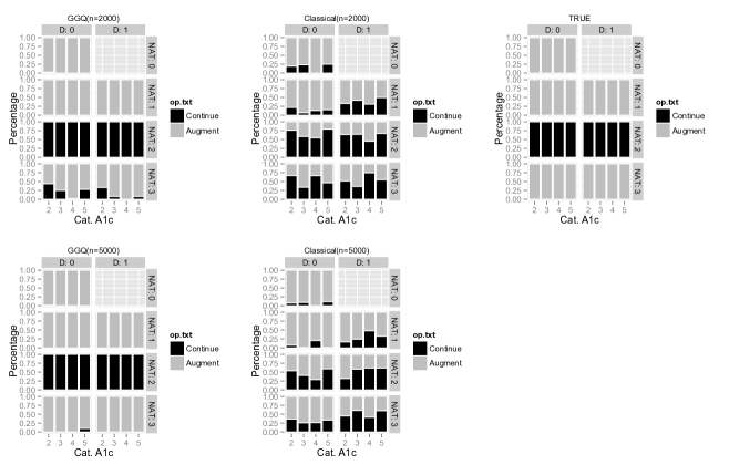
Figure 1: Simulation: Estimated optimal treatment (op.txt) for different states. The shaded bar represents the evidence in the simulated data for each of the treatment choices as labeled in the legend. The upper and lower horizontal axes are the discontinuation indicator and the categorized A1c (Cat.A1c), respectively. The vertical axes on the right and left hand side give $NAT$ and the percentage of time that the treatment choices are selected as the optimal choice.

Unlike the classical approach, the optimal treatment policy using our proposed GGQ method utilizes the continuous state variable $S_{t}=(NAT_{t},D_{t},A1c_{t},BP_{t},Weight_{t})$. In our example, we parametrize the optimal action value function $Q^{*}(s,a)$ using a 72-dimensional vector of parameters and construct the features $\varphi(s,a)$ using radial basis functions (Gaussian kernels). See Appendix 2 for more details. To specify the step sizes of the stochastic minimization algorithm, first we select two functions that satisfy the conditions $P.1-4$ listed in Appendix 1 and multiply them by $v\in(0,1)$. Then we run the algorithm for different values of $v$ and select the one that minimizes the objective function. In this simulation study we set the step sizes $\alpha_{k}=\nu/(k\log(k))$ and $\beta_{k}=\nu/k$ where $\nu$ is set to 0.05. Section S5 in the supplementary materials discusses the effect of the choice of tuning parameters on the estimated optimal regime.

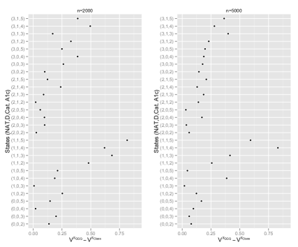
Figure 2: Simulation: Monte Carlo approximation of the difference between value functions. $V^{\pi_{GGQ}}$ and $V^{\pi_{Class}}$ are the value functions corresponding to the classical and GGQ approaches. The vertical axis represents the triplets of states in the order of $(NAT,D,Cat.A1c)$.

True optimal policy. As the sample size increases, the optimal action-value function estimated using the classical approach converges to the true optimal action-value function. Hence, for the purpose of finding the true optimal policy, we generate a large dataset of size 500,000 and estimate transition probabilities $P_{S^{\prime}|S,A}$ using a nonparametric approach, where $S$ is the oracle state $(NAT_{t},D_{t},Cat.A1c_{t})$. Then by the 5-step procedure (classical approach), the true optimal policy is approximated and set as our benchmark.

Figure 1 depicts the true and estimated optimal treatment for each discretized oracle state $(NAT_{t},D_{t},Cat.A1c_{t})$ using the GGQ and classical approaches. As in this example, we set the discount factor $\gamma$ to 0.6. Note that the estimated optimal policy using classical and GGQ methods is based on the states $S^{Class}_{t}$ and $S_{t}$, respectively. However, in Figure 1, we averaged it over the noise variables $(BP,Weight)$ and, for comparability, we report the results on the discretized oracle state. The vertical axis on the left hand side is the percentage of time that the treatment choices are selected as optimal. The left vertical and both horizontal axes represent the elements of the state $(NAT,D,Cat.A1c)$, respectively. This plot shows that the proposed GGQ method outperforms the classical approach for moderate sample sizes.

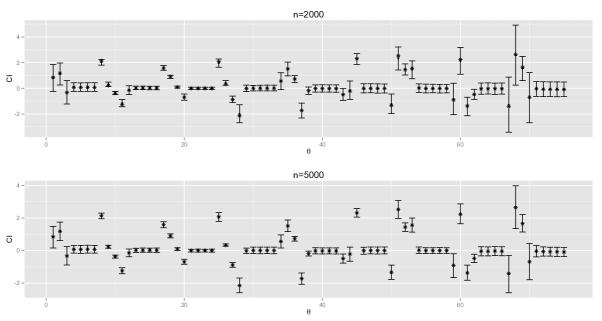
Figure 3: Simulation: Plot of the 95% confidence intervals of $\theta$.

More specifically, the estimated optimal policy using GGQ ($\hat{\pi}_{GGQ}$) recommends not augmenting the third (glitazone^∗) and fourth (insulin) treatments (the left plots). This makes sense since glitazone^∗ has a small treatment effect (0.02) and insulin has high discontinuation rate (0.35) that outweighs its efficacy. However, the estimated optimal policy using a classical approach ($\hat{\pi}_{Class}$) recommends augmenting these treatments by some positive probabilities. Specifically, $\hat{\pi}_{Class}$ augments insulin about 50% of the time when $D=1$ and $Cat.A1c\in\{2,3,4\}$.

Figure 2 presents the difference between the values of the estimated optimal policies $\hat{\pi}_{GGQ}$ and $\hat{\pi}_{Class}$. The values are calculated using the Monte Carlo method, where the value of a treatment policy $\pi$, for each state $s$, is defined as $V^{\pi}(s)=\mathbbmss{E}_{\pi}\left[\sum_{k=1}^{\infty}\gamma^{k-1}R_{t+k}|S_{t}=s,A_{t}=\pi(s)\right]$. For both sample sizes and all of the states, the value of $\hat{\pi}_{GGQ}$ is higher than the value of $\hat{\pi}_{Class}$. This indicates that the estimated optimal policy $\hat{\pi}_{GGQ}$ has better quality.

Our simulation result is consistent with Timbie et al. (2010), and suggests that we should not always augment the treatment when $7<A1c<8$. In other words, depending on the treatment already taken, sometimes we should consider not augmenting the treatment to avoid side effects.

4.4 Monte Carlo studies

We generate 500 datasets each of sizes 2,000 and 5,000 to examine the asymptotic behavior of the proposed method. Figure 3 shows the confidence intervals of $\theta$, where the standard errors are estimated using the variance formula presented in Theorem 3.1. The dark circles are the average of the 500 $\hat{\theta}$s and asterisks are the true parameter values approximated using a Monte Carlo study with $n=10,000$. These confidence intervals may be used to identify the parts of the feature function that should be kept in the decision rule and may be used as a feature selection tool. Another important use of the asymptotic results in Theorem 1 is to investigate whether there is a significant difference between treatment options. Specifically, one may build the confidence interval for the difference between the estimated optimal action-value function for different treatment options (augment vs. continue) and check whether it contains zero (while adjusting for Type-I error rate for more than two treatment options). In Figure 4, we constructed and evaluated the quality of these 95% confidence intervals for $Q^{*}(s,augment)-Q^{*}(s,0)$, given each state variable for $n=2000$. The results for $n=5000$ is similar and omitted due to space limitations. These results confirm the accuracy of our variance estimator in Theorem 1.

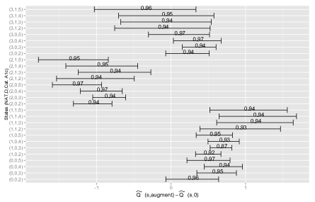
Figure 4: Simulation: The confidence intervals of the difference between the estimated optimal action-value function when the treatment is augmented and continued (i.e., $\hat{Q}^{*}(s,augment)-\hat{Q}^{*}(s,0)$). The number on each confidence interval represents the coverage of that interval. The vertical axis represents the triplets of states in the order of $(NAT,D,Cat.A1c)$.

5 Discussion

We have proposed a new method that can be used to form optimal dynamic treatment regimes in infinite-horizon settings (i.e., there is no a priori fixed end of follow up), while our data were collected over a fixed period of time with many decision points. We have assumed that the value of the optimal regime can be presented using a linear function of parameters, and we developed an estimating procedure based on temporal difference residuals to estimate the parameters of this function. We developed the asymptotic properties of the estimated parameters and evaluated the proposed method using simulation studies.

This work raises a number of interesting issues. We have derived the asymptotic distribution of the estimators under some assumptions. One important practical problem is to provide a valid inference when the optimal treatment is not unique for some states, (i.e., assumption $A.8$ is violated). This may lead to non-regular estimators and inflate the Type-I error rate (Bickel et al., 1993). Among others, Robins (2004) and Laber et al. (2010) proposed solutions to this issue. However, the existing methods may not be directly applied to our method and require major modifications. The second issue is how to construct the feature functions. In this manuscript, we used the radial basis functions (Moody & Darken, 1989; Poggio & Girosi, 1990). One simple method is to try different feature functions ($\varphi$) and select the one that minimizes the function $f(\varphi)=\min_{\theta}M(\theta)$ (Parr et al., 2008). Alternatively, one may use support vector regression to approximate the action-value function (Vapnik et al., 1997; Tang & Kosorok, 2012).

The proposed method can be used in settings where the time between decision points is fixed, say 3 months. This assumption often holds (approximately) for some chronic diseases such as diabetes, cyclic fibrosis and asthma. It would, however, be of interest to extend the method to cases with a random decision point (clinic visits). Usually, the random time between decision points happens either when doctors decide to schedule the next visit sooner or later than the prespecified time or when patients request an appointment due to, for example, side effects or acute symptoms. The former is easier to deal with because we have the covariates required to model the visit process. The latter, however, is more difficult and results in non-ignorable missing data because we do not have information about those patients who did not show up. Robins et al. (2008) discusses the issue of the random visit process in detail.

Supplementary material

Supplementary material available at Biometrika  online includes the stochastic minimization algorithm and proof of Theorem 1. It also discusses the effect of the discount factor and tuning parameters of the stochastic minimization algorithm on the estimated optimal treatment regime.

Appendix 1: Tuning Parameters

The tuning parameters $\alpha_{k}$ and $\beta_{k}$ in the GGQ algorithm need to satisfy the following assumptions (Maei et al., 2010):

1. $\alpha_{k}$, $\beta_{k}$ $\forall k$ and are deterministic.

2. $\sum_{k=0}^{\infty}\alpha_{k}=\sum_{k=0}^{\infty}\beta_{k}=\infty$.

3. $\sum_{k=0}^{\infty}(\alpha_{k}^{2}+\beta_{k}^{2})<\infty$.

4. $\alpha_{k}/\beta_{k}\rightarrow 0$.

Appendix 2: feature functions

The feature functions are constructed using the radial basis functions and

$$\varphi(s,a)=I(s\neq\emptyset)(\varphi_{1}(s,a),\varphi_{2}(s,a),\varphi_{3}(s,a),\varphi_{4}(s,a),\varphi_{5}(s,a),\varphi_{6}(s,a),\varphi_{7}(s,a),\varphi_{8}(s,a),\varphi_{9}(s,a)),$$

where

$$\varphi_{1}(s,a) =I(A=0,NAT=0)(1,\exp[-h(A1c-q_{11})^{2}],\exp[-h(A1c-q_{12})^{2}],\phi(BP),\phi(Weight))$$

$$\varphi_{2}(s,a) =I(A=0,NAT=1)(1,\exp[-h(A1c-q_{21})^{2}],\exp[-h(A1c-q_{22})^{2}],\exp[-h(A1c-8.0)^{2}],$$

$$\hskip 289.07999ptd,\phi(BP),\phi(Weight))$$

$$\varphi_{3}(s,a) =I(A=0,NAT=2)(1,\exp[-h(A1c-q_{31})^{2}],\exp[-h(A1c-q_{33})^{2}],d,\phi(BP),\phi(Weight))$$

$$\varphi_{4}(s,a) =I(A=0,NAT=3)(1,\exp[-h(A1c-q_{41})^{2}],\exp[-h(A1c-q_{42})^{2},\exp[-h(A1c-8.5)^{2}],$$

$$\hskip 289.07999ptd,\phi(BP),\phi(Weight))$$

$$\varphi_{5}(s,a) =I(A=0,NAT=4)(1,\exp[-h(A1c-q_{51})^{2}],\exp[-h(A1c-q_{52})^{2},\exp[-h(A1c-8.0)^{2}],$$

$$\hskip 289.07999ptd,\phi(BP),\phi(Weight))$$

$$\varphi_{6}(s,a) =I(A=1,NAT=0)(1,\exp[-h(A1c-6.5)^{2}],\exp[-h(A1c-7.5)^{2}],\phi(BP),\phi(Weight))$$

$$\varphi_{7}(s,a) =I(A=2,NAT=1)(1,\exp[-h(A1c-6.5)^{2}],\exp[-h(A1c-q_{71})^{2}],\exp[-h(A1c-q_{73})^{2}]$$

$$\hskip 289.07999ptd,\phi(BP),\phi(Weight))$$

$$\varphi_{8}(s,a) =I(A=3,NAT=2)(1,\exp[-h(A1c-q_{82})^{2}],\exp[-h(A1c-8.5)^{2}],d,\phi(BP),\phi(Weight))$$

$$\varphi_{9}(s,a) =I(A=4,NAT=3)(1,\exp[-h(A1c-6.5)^{2}],\exp[-h(A1c-q_{92})^{2},\exp[-h(A1c-8.5)^{2}],$$

$$\hskip 289.07999ptd,\phi(BP),\phi(Weight)),$$

where $\phi(BP)=(\exp[-h(BP-q_{b1})^{2}],\exp[-h(BP-q_{b3})^{2}])$ and $\phi(Weight)=(\exp[-h(Weight-q_{w1})^{2}],\exp[-h(Weight-q_{w3})^{2}]).$ $h$ is a positive constant and $q_{.j}$ is the observed $jth$ quantile of the corresponding variable. For example, $q_{11}$ and $q_{12}$ are the first and second quantiles of $A1c$ given $A=0$ and $NAT=0$. Similarly, $q_{b1}$ and $q_{b3}$ are the first and third quantiles of $BP$. Note that, in our generative model, $BP$ and $Weight$ are independent of $A$ and $NAT$.

Remark 1. Number of quantiles used in each $\varphi_{k}$ and $\phi(.)$ is a bias-variance trade-off such that increasing the number of quantiles decreases the bias but increases the variance of the estimated parameters. Similarly, decreasing the value of $h$ may decrease the bias but increase the variance of the estimators. In our simulation, we set $h=0.5$.

Appendix 3: Assumptions

In addition to assumptions A.1-3, the following assumptions are required for large sample properties of our estimator.

• A.4 $\theta_{0}^{\top}\varphi(.,.)$ is the optimal Q-function.

• A.5 $\mathbbmss{E}\left[\sum_{t=0}^{T-1}\|\varphi(S_{t},A_{t})\|_{2}\|\varphi(S_{t},a)\|_{2}\right]<\infty$, for any $a\in\mathcal{A}$.

• A.6 The matrix $W$ is of full rank.

• A.7 $\mathbbmss{E}\left[\sum_{t=0}^{T-1}\left\{\gamma I_{|\pi^{*}(S_{t+1})|=1}\varphi(S_{t+1},\pi^{*}(S_{t+1}))-\varphi(S_{t},A_{t})\right\}\varphi(S_{t},A_{t})^{\top}\right]$ is of full rank where $\pi^{*}(S_{t+1})=\arg\max_{a}\theta_{0}^{\top}\varphi(S_{t+1},a)$ and $|.|$ is the cardinal of a set.

• A.8 The optimal treatment is unique at each decision point.

Web-based Supplementary Materials for
“Constructing Dynamic Treatment Regimes in Infinite-Horizon Settings”

S1. The stochastic minimization algorithm

We base our minimization procedure on the (approximate) gradient descent approach, in which sub-gradients are defined as Frechet sub-gradients of the objective function $M(\theta)$. Following Maei et al. (2010) and under under assumptions A.1-8, the algorithm converges to the minimizer of our objective function.

The sub-gradient $\partial M(\theta)$ of $M(\theta)$ with respect to $\theta$ is

$$\partial M(\theta)=-\mathbbmss{E}\left[\sum_{t}\delta_{t+1}(\theta)\varphi(s_{t},a_{t})^{\top}\right]+\gamma\mathbbmss{E}\left[\sum_{t}\varphi(s_{t+1},\pi^{*}(s_{t+1}))\varphi(s_{t},a_{t})^{\top}\right]\varpi,$$

where $\varpi=\mathbbmss{E}[\sum_{t}\varphi(s_{t},a_{t})\varphi(s_{t},a_{t})^{\top}]^{-1}\mathbbmss{E}[\sum_{t}\delta_{t+1}(\theta)\varphi(s_{t},a_{t})^{\top}]$. Using the weight-doubling trick introduced by Sutton et al. (2009b), we summarize the steps toward minimizing the objective function $M(\theta)$ as follows:

• Set initial values for the $p$ dimensional vectors of $\theta$ and $\varpi$. Using grid search, the initial value $\theta_{1}$ can be set as the one that minimizes the objective function and the initial value $w_{1}=\mathbbmss{P}_{n}[\sum_{t}\varphi(s_{t},a_{t})\varphi(s_{t},a_{t})^{\top}]^{-1}\mathbbmss{P}_{n}[\sum_{t}\delta_{t+1}(\theta_{0})\varphi(s_{t},a_{t})^{\top}]$.

• Start from the first individual’s trajectory and obtain $\theta_{k+1}$ from the following iterative equations:

  $$\theta_{k+1} =\theta_{k}+\alpha_{k}\nu\sum_{t}\left[\delta_{t+1}(\theta_{k})\varphi(s_{t},a_{t})-\gamma\{\varpi_{k}^{\top}\varphi(s_{t},a_{t})\}\varphi(s_{t+1},\pi^{*}_{\theta_{k}}(s_{t+1}))^{\top}\right]$$ (11)

  $$\varpi_{k+1} =\varpi_{k}+\beta_{k}\nu\sum_{t}\left[\delta_{t+1}(\theta_{k})-\{\varphi(s_{t},a_{t})^{\top}\varpi_{t}\}^{\top}\right]\varphi(s_{t},a_{t})^{\top},$$ (12)

  where $\alpha_{k}$, $\beta_{k}$ and $\nu$ are tuning parameters (step sizes) and $\pi^{*}_{\theta_{k}}(.)$ is the optimal policy estimated as a function of $\theta_{k}$.

• Use step 2 to continue updating the parameters to the last individual.

• Continue steps 2 and 3 until $\|\theta_{k+1}-\theta_{k}\|_{2}<c$ where $c$ is a constant.

The tuning parameters (step sizes) $\alpha_{k}$ and $\beta_{k}$ need to satisfy assumptions P.1-P.4 in Appendix A. The parameter $\nu$ tunes the step sizes and lies in the interval (0,1). Our simulation studies show that the best choice of $\nu$ would be close to $\frac{1}{T}$, where $T$ is the maximal length of the trajectories in our data. See our discussion in Section S5.

S2. Lemma

Lemma .1.

Let $\{a_{i}\}_{1}^{K}$ and $\{b_{i}\}_{1}^{K}$ be two sets of elements, then

1. $\lim_{\|b\|\rightarrow 0}\frac{\max_{1\leq i\leq K}[a_{i}+b_{i}]-\max_{i\in\pi^{*}}[a_{i}+b_{i}]}{\|b\|}=0$;

2. $\max_{1\leq i\leq K}[a_{i}+b_{i}]-\max_{i\in\pi^{*}}[a_{i}+b_{i}]$ is non-negative and bounded above by

   $$\max_{i\notin\pi^{*}}b_{i}-\max_{i\in\pi^{*}}b_{i}\leq\max_{1\leq i\leq K}b_{i}-\max_{i\in\pi^{*}}b_{i}$$

   where $\pi^{*}=\arg\max_{1\leq i\leq K}a_{i}$.

Proof .2.

Part I. Since the set $\pi^{*}$ is a subset of $1\leq i\leq K$, we have

$$0 \leq\frac{\max_{1\leq i\leq K}[a_{i}+b_{i}]-\max_{i\in\pi^{*}}[a_{i}+b_{i}]}{\|b\|}$$

$$=\max_{1\leq i\leq K}\left[a_{i}-a_{i^{*}}+b_{i}-\max_{i\in\pi^{*}}b_{i}\right]\frac{1}{\|b\|},\hskip 36.135pt\text{ $\forall i^{*}\in\pi^{*}$ }$$

$$=\max\left[\max_{i\in\pi^{*}}\{b_{i}-\max_{i\in\pi^{*}}b_{i}\},\max_{i\notin\pi^{*}}\{a_{i}-a_{i^{*}}+b_{i}-\max_{i\in\pi^{*}}b_{i}\}\right]\frac{1}{\|b\|}$$

$$=\max\left[0,\max_{i\notin\pi^{*}}\left\{\frac{a_{i}-a_{i^{*}}}{\|b\|}+\frac{b_{i}-\max_{i\in\pi^{*}}b_{i}}{\|b\|}\right\}\right]$$

$$\leq\max\left[0,\max_{i\notin\pi^{*}}\left\{\frac{a_{i}-a_{i^{*}}}{\|b\|}+\frac{2|\max_{1\leq i\leq K}b_{i}|}{\|b\|}\right\}\right]$$

Since $\frac{a_{i}-a_{i^{*}}}{\|b\|}\rightarrow-\infty$ as $\|b\|\rightarrow 0$ and $\frac{|\max_{i\in\pi}b_{i}|}{\|b\|}\leq 1$, part I is proved. Part II can be proved similarly.

S3. Proof of Theorem 1

We first show that the objective function $M(\theta)$ is continuous. Then using the results of Lemma .1, we show that $M(\theta)$ satisfies the two required conditions of Theorem 3.2.1 in Van Der Vaart & Wellner (1996), which completes the proof of consistency. To prove the asymptotic normality, under the additional assumption $A.8$, we define a function $V(b)$ such that $\sqrt{n}(\hat{\theta}-\theta_{0})\rightarrow_{d}\arg\min_{b}V(b)$, where $\arg\min_{b}V(b)$ is normally distributed.

First, we show that the function $M(\theta)$ is continuous by proving the continuity of $D(\theta)$ around $\theta=\theta_{0}$. Since

$$\|D(\theta)-D(\theta_{0})\| =\|\sum_{t=0}^{T-1}\mathbbmss{E}\left[\{\max_{a}[\theta^{\top}\varphi(S_{t+1},a)]-\max_{a}[\theta_{0}^{\top}\varphi(S_{t+1},a)]\right.$$

$$\hskip 144.54pt\left.-\theta^{\top}\varphi(S_{t},A_{t})+\theta_{0}^{\top}\varphi(S_{t},A_{t})\}\varphi(S_{t},A_{t})^{\top}\right]\|,$$

by the Cauchy-Schwartz inequality and the fact that $|\max_{a}f(a)-\max_{a}g(a)|\leq\max_{a}|f(a)-g(a)|$, we have

$$\mathbbmss{E}\left[\max_{a}[\theta^{\top}\varphi(S_{t+1},a)]-\max_{a}[\theta_{0}^{\top}\varphi(S_{t+1},a)]\right]\leq||\theta-\theta_{0}||\mathbbmss{E}\left[\sum_{a}\|\varphi(S_{t+1},a)\|\right],$$

which under assumption $A.4$ implies the continuity of $D(\theta)$ around $\theta=\theta_{0}$.

Part I (Consistency). We show that $M(\theta)$ satisfies the two conditions listed in Theorem 3.2.1 Van Der Vaart and Wellner (1996). For the first condition, we need to show that for some $\epsilon>0$ and $c>0$ with $||\theta-\theta_{0}||<\epsilon$,

$$D(\theta_{0})W^{-1}D(\theta_{0})^{\top}-D(\theta)W^{-1}D(\theta)^{\top}\leq-c||\theta-\theta_{0}||^{2},$$

and since $D(\theta_{0})=0$,

$$D(\theta)W^{-1}D(\theta)^{\top}\geq c||\theta-\theta_{0}||^{2}.$$ (13)

The left hand side of the above inequality can be written as

$$D(\theta)W^{-1}D(\theta)^{\top} =[D(\theta)-D(\theta_{0})-\dot{D}_{\theta_{0}}(\theta-\theta_{0})]W^{-1}[D(\theta)-D(\theta_{0})-\dot{D}_{\theta_{0}}(\theta-\theta_{0})]^{\top}$$

$$+\dot{D}_{\theta_{0}}(\theta-\theta_{0})W^{-1}\dot{D}_{\theta_{0}}(\theta-\theta_{0})^{\top}+2\dot{D}_{\theta_{0}}(\theta-\theta_{0})W^{-1}[D(\theta)-D(\theta_{0})-\dot{D}_{\theta_{0}}(\theta-\theta_{0})]^{\top},$$

where

$$\dot{D}_{\theta_{0}}(b)=\mathbbmss{E}\left[\sum_{t=0}^{T-1}\{\gamma\max_{a\in\pi^{*}(S_{t+1})}b^{\top}\varphi(S_{t+1},a)-b^{\top}\varphi(S_{t},A_{t})\}\varphi(S_{t},A_{t})^{\top}\right],$$

and $\pi^{*}(S_{t+1})=\arg\max_{a}\theta_{0}^{\top}\varphi(S_{t+1},a)$. Note that $\pi^{*}(S_{t+1})$ may be a set of actions. Now, we show that $\|D(\theta)-D(\theta_{0})-\dot{D}_{\theta_{0}}(\theta-\theta_{0})\|=o(\|\theta-\theta_{0}\|)$.

$$\frac{\|D(\theta)-D(\theta_{0})-\dot{D}_{\theta_{0}}(\theta-\theta_{0})\|}{\|\theta-\theta_{0}\|}=$$

$$\frac{\gamma}{||\theta-\theta_{0}||}\left\|\mathbbmss{E}\left[\sum_{t=0}^{T-1}\left\{\max_{a}(\theta_{0}+b||\theta-\theta_{0}||)^{\top}\varphi(S_{t+1},a)-\max_{a\in\pi^{*}(S_{t+1})}\theta_{0}^{\top}\varphi(S_{t+1},a)\right.\right.\right.$$

$$\hskip 216.81pt\left.\left.\left.-\max_{a\in\pi^{*}(S_{t+1})}b^{\top}\varphi(S_{t+1},a)\|\theta-\theta_{0}\|\right\}\varphi(S_{t},A_{t})^{\top}\right]\right\|,$$

where $b=(\theta-\theta_{0})/\|\theta-\theta_{0}\|$. Then, since $\forall a,a^{\prime}\in\pi^{*}(S_{t+1})$, we have $\theta_{0}^{\top}\varphi(S_{t+1},a)=\theta_{0}^{\top}\varphi(S_{t+1},a^{\prime})$. Thus the following equality holds:

$$\max_{a\in\pi^{*}(S_{t+1})}\theta_{0}^{\top}\varphi(S_{t+1},a)+\max_{a\in\pi^{*}(S_{t+1})}(\theta-\theta_{0})^{\top}\varphi(S_{t+1},a)=\max_{a\in\pi^{*}(S_{t+1})}\theta^{\top}\varphi(S_{t+1},a).$$

Thus,

$$\frac{||D(\theta)-D(\theta_{0})-\dot{D}_{\theta_{0}}(\theta-\theta_{0})||}{||\theta-\theta_{0}\|}=$$

$$\frac{\gamma}{||\theta-\theta_{0}||}\left\|\mathbbmss{E}\left[\sum_{t=0}^{T-1}\left\{\max_{a}(\theta_{0}+b||\theta-\theta_{0}||)^{\top}\varphi(S_{t+1},a)-\max_{a\in\pi^{*}(S_{t+1})}(\theta_{0}+b\|\theta-\theta_{0}\|)^{\top}\varphi(S_{t+1},a)\right\}\varphi(S_{t},A_{t})^{\top}\right]\right\|$$

$$\leq\gamma\mathbbmss{E}\left[\sum_{t=0}^{T-1}\|\varphi(S_{t+1},a)\|\left\{\max_{a}\left(\frac{\theta_{0}}{||\theta-\theta_{0}||}+b\right)^{\top}\varphi(S_{t+1},a)-\max_{a\in\pi^{*}(S_{t+1})}\left(\frac{\theta_{0}}{\|\theta-\theta_{0}\|}+b\right)^{\top}\varphi(S_{t+1},a)\right\}\right]$$

$$\leq\gamma\mathbbmss{E}\left[\sum_{t=0}^{T-1}\|\varphi(S_{t},A_{t})\|\left\{\max_{a}b^{\top}\varphi(S_{t+1},a)-\max_{a\in\pi^{*}(S_{t+1})}b^{\top}\varphi(S_{t+1},a)\right\}\right]$$

$$\leq\gamma\mathbbmss{E}\left[\sum_{t=0}^{T-1}\|\varphi(S_{t},A_{t})\|\sum_{a\in\mathcal{A}_{S_{t+1}}}\|b\|\|\varphi(S_{t+1},a)\|\right]<\infty.$$

The second inequality follows from Lemma .1 part (II) and the last inequality follows from $\|b\|=1$ and assumption A.5. Also, using Lemma .1 part (I), we have

$$\lim_{\|\theta-\theta_{0}\|\rightarrow 0}\left[\max_{a}\left(\frac{\theta_{0}}{||\theta-\theta_{0}||}+b\right)^{\top}\varphi(S_{t+1},a))-\max_{a\in\pi^{*}(S_{t+1})}\left(\frac{\theta_{0}}{\|\theta-\theta_{0}\|}+b\right)^{\top}\varphi(S_{t+1},a)\right]=0.$$

We just showed that $\|D(\theta)-D(\theta_{0})-\dot{D}_{\theta_{0}}(\theta-\theta_{0})\|=o(\|\theta-\theta_{0}\|)$. Since $W^{-1}$ is of full rank matrix,

$$[D(\theta)-D(\theta_{0})-\dot{D}_{\theta_{0}}(\theta-\theta_{0})]W^{-1}[D(\theta)-D(\theta_{0})-\dot{D}_{\theta_{0}}(\theta-\theta_{0})]^{\top}=o(\|\theta-\theta_{0}\|^{2}).$$

Now, we need to show that $\dot{D}_{\theta_{0}}(\theta-\theta_{0})\dot{D}_{\theta_{0}}(\theta-\theta_{0})^{\top}\geq c^{\prime\prime}\|\theta-\theta_{0}\|^{2}$. By definition,

$$\dot{D}_{\theta_{0}}(\theta-\theta_{0}) =\mathbbmss{E}\left[\sum_{t=0}^{T-1}\left\{\gamma\max_{a\in\pi^{*}(S_{t+1})}(\theta-\theta_{0})^{\top}\varphi(S_{t+1},a)-(\theta-\theta_{0})^{\top}\varphi(S_{t},A_{t})\right\}\varphi(S_{t},A_{t})^{\top}\right]$$

$$=(\theta-\theta_{0})^{\top}\mathbbmss{E}\left[\sum_{t=0}^{T-1}\left\{\gamma I_{|\pi^{*}(S_{t+1})|=1}\varphi(S_{t+1},\pi^{*}(S_{t+1}))-\varphi(S_{t},A_{t})\right\}\varphi(S_{t},A_{t})^{\top}\right]$$

$$+\gamma\mathbbmss{E}\left[\sum_{t=0}^{T-1}\left\{\gamma I_{|\pi^{*}(S_{t+1})|>1}\max_{a\in\pi^{*}(S_{t+1})}\frac{(\theta-\theta_{0})^{\top}}{\|\theta-\theta_{0}\|}\varphi(S_{t+1},a)\right\}\varphi(S_{t},A_{t})^{\top}\right]\|\theta-\theta_{0}\|.$$

Let

$$M_{1} =\mathbbmss{E}\left[\sum_{t=0}^{T-1}\left\{\gamma I_{|\pi^{*}(S_{t+1})|=1}\varphi(S_{t+1},\pi^{*}(S_{t+1}))-\varphi(S_{t},A_{t})\right\}\varphi(S_{t},A_{t})^{\top}\right],$$

$$M_{2} =\mathbbmss{E}\left[\sum_{t=0}^{T-1}\left\{I_{|\pi^{*}(S_{t+1})|>1}\max_{a\in\pi^{*}(S_{t+1})}\frac{(\theta-\theta_{0})^{\top}}{\|\theta-\theta_{0}\|}\varphi(S_{t+1},a)\right\}\varphi(S_{t},A_{t})^{\top}\right].$$

Then

$$\dot{D}_{\theta_{0}}(\theta-\theta_{0})\dot{D}_{\theta_{0}}(\theta-\theta_{0})^{\top}=(\theta-\theta_{0})^{\top}M_{1}M_{1}^{\top}(\theta-\theta_{0})+2\gamma(\theta-\theta_{0})^{\top}M_{1}M_{2}^{\top}\|\theta-\theta_{0}\|+\gamma^{2}\|\theta-\theta_{0}\|^{2}M_{2}M_{2}^{\top}.$$

Assuming that $M_{1}$ is of full rank (Assumption A.7), we have

$$(\theta-\theta_{0})^{\top}M_{1}M_{1}^{\top}(\theta-\theta_{0})\geq\|\theta-\theta_{0}\|^{2}\lambda_{min},$$

where $\lambda_{min}$ is the smallest eigenvalue of $M_{1}^{\top}M_{1}$. Also, using singular value decomposition we have

$$(\theta-\theta_{0})^{\top}M_{1}M_{2}^{\top}\|\theta-\theta_{0}\|\leq\|\theta-\theta_{0}\|^{2}\sqrt{\lambda_{max}}\|M_{2}\|,$$

where $\lambda_{max}$ is a maximum eigenvalue of $M_{1}M_{1}^{\top}$. Thus

$$\dot{D}_{\theta_{0}}(\theta-\theta_{0})\dot{D}_{\theta_{0}}(\theta-\theta_{0})^{\top}\geq\|\theta-\theta_{0}\|^{2}\left[\lambda_{min}-2\gamma\sqrt{\lambda_{max}}\|M_{2}\|-\gamma^{2}\|M_{2}\|^{2}\right].$$

Therefore, function $M(.)$ satisfies the first condition of Theorem 3.2.5 in Van Der Vaart and Wellner (1996) for any small enough $\gamma$ such that $\left[\lambda_{min}-2\gamma\sqrt{\lambda_{max}}\|M_{2}\|-\gamma^{2}\|M_{2}\|^{2}\right]>0$. Note that under assumption $A.8$ when $|\pi^{*}(S_{t+1})|=1$, the latter condition is satisfied automatically. Since $W$ is of full rank (Assumption $A.6$), $\dot{D}_{\theta_{0}}(\theta-\theta_{0})W^{-1}\dot{D}_{\theta_{0}}(\theta-\theta_{0})^{\top}\geq c\|\theta-\theta_{0}\|^{2}$ for $c>0$.

For the second condition, we need to show that for every large enough $n$, sufficiently small $\delta_{n}$ and $c>0$

$$\mathbbmss{E}\sup_{\|\theta-\theta_{0}\|\leq\delta_{n}}\left|[\hat{M}(\theta)-M(\theta)]-[\hat{M}(\theta_{0})-M(\theta_{0})]\right|\leq c\delta_{n}^{2}.$$

Since by definition $\hat{D}(\hat{\theta})=D(\theta_{0})=0$, we have

$$\left|[\hat{M}(\theta)-M(\theta)]-[\hat{M}(\theta_{0})-M(\theta_{0})]\right|= \left|(\hat{D}(\theta)-\hat{D}(\hat{\theta}))\hat{W}^{-1}(\hat{D}(\theta)-\hat{D}(\hat{\theta}))^{\top}\right.$$

$$-(\hat{D}(\theta_{0})-\hat{D}(\hat{\theta}))\hat{W}^{-1}(\hat{D}(\theta_{0})-\hat{D}(\hat{\theta}))^{\top}$$

$$\left.-(D(\theta)-D(\theta_{0}))\hat{W}^{-1}(D(\theta)-D(\theta_{0}))^{\top}\right|.$$

We show that for every large $n$ such that $\|\theta-\hat{\theta}\|\leq\delta_{n}$ and $\|\theta_{0}-\hat{\theta}\|\leq\delta_{n}$

$$\mathbbmss{E}\sup_{\|\theta-\hat{\theta}\|\leq\delta_{n}}[(\hat{D}(\theta)-\hat{D}(\hat{\theta}))\hat{W}^{-1}(\hat{D}(\theta)-\hat{D}(\hat{\theta}))^{\top}]\leq c_{1}\delta_{n}^{2}$$

$$\mathbbmss{E}\sup_{\|\hat{\theta}-\theta_{0}\|\leq\delta_{n}}[(\hat{D}(\theta_{0})-\hat{D}(\hat{\theta}))\hat{W}^{-1}(\hat{D}(\theta_{0})-\hat{D}(\hat{\theta}))^{\top}]\leq c_{2}\delta_{n}^{2}$$

$$\mathbbmss{E}\sup_{\|\theta-\theta_{0}\|\leq\delta_{n}}[(D(\theta)-D(\theta_{0}))^{\top}\hat{W}^{-1}(D(\theta)-D(\theta_{0}))^{\top}]\leq c_{3}\delta_{n}^{2},$$

where $c_{1}$, $c_{2}$ and $c_{3}$ are positive constants. Here we show the first inequality and the rest can be shown similarly. By the Cauchy-Schwartz inequality and the fact that $|\max_{a}f(a)-\max_{a}g(a)|\leq\max_{a}|f(a)-g(a)|$, we have

$$|\hat{D}(\theta)-\hat{D}(\hat{\theta})|= \left|\mathbbmss{P}_{n}\left[\sum_{t=0}^{T-1}\left\{\max_{a}\theta^{\top}\varphi(S_{t+1},a)-\max_{a}\hat{\theta}^{\top}\varphi(S_{t+1},a)-(\theta-\hat{\theta})^{\top}\varphi(S_{t},A_{t})\right\}\varphi(S_{t},A_{t})^{\top}\right]\right|$$

$$\leq\mathbbmss{P}_{n}\left[\sum_{t=0}^{T-1}\|\varphi(S_{t},A_{t})\|\left\{\sum_{a}\|\varphi(S_{t+1},a)\|\|\theta-\hat{\theta}\|+\|\varphi(S_{t},A_{t})\|\|\theta-\hat{\theta}\|\right\}\right].$$

Thus,

$$|\hat{D}(\theta)-\hat{D}(\hat{\theta})|\leq m(S,A)\|\theta-\hat{\theta}\|,$$

where

$$m(S,A)=\mathbbmss{P}_{n}\left[\sum_{t=0}^{T-1}\|\varphi(S_{t},A_{t})\|\left\{\sum_{a}\|\varphi(S_{t+1},a)\|+\|\varphi(S_{t},A_{t})\|\right\}\right].$$

Therefore

$$\mathbbmss{E}\sup_{\|\theta-\hat{\theta}\|\leq\delta_{n}}[(\hat{D}(\theta)-\hat{D}(\hat{\theta}))^{\top}\hat{W}^{-1}(\hat{D}(\theta)-\hat{D}(\hat{\theta}))]\leq c_{1}\delta_{n}^{2},$$

where $c_{1}=\mathbbmss{E}[m(S,A)^{2}\|\hat{W}^{-1}\|]$. Define $c=c_{1}+c_{2}+c_{3}$. This shows that our objective function satisfies the second condition of Theorem 3.2.5 in Van Der Vaart and Wellner (1996) as well. This completes the proof of consistency.

Part II (Asymptotic Normality). Let $\theta=\theta_{0}+\frac{b}{\sqrt{n}}$ and

$$\hat{V}(b)=n\hat{D}(\theta_{0}+b/\sqrt{n})\hat{W}^{-1}\hat{D}(\theta_{0}+b/\sqrt{n})^{\top}-n\hat{D}(\theta_{0})\hat{W}^{-1}\hat{D}(\theta_{0})^{\top}.$$

Then,

$$\hat{D}(\theta_{0}+b/\sqrt{n}) =\mathbbmss{P}_{n}\left[\sum_{t}\left\{R_{t+1}+\gamma\max_{a}\theta_{0}^{\top}\varphi(S_{t+1},a)-\theta_{0}^{\top}\varphi(S_{t},A_{t})-b^{\top}/\sqrt{n}\varphi(S_{t},A_{t})\right.\right.$$

$$\hskip 72.26999pt\left.-\gamma\max_{a}\theta_{0}^{\top}\varphi(S_{t+1},a)+\gamma\max_{a}(\theta_{0}+b/\sqrt{n})^{\top}\varphi(S_{t+1},a)\right\}\varphi(S_{t},A_{t})^{\top}\Bigg{]}$$

$$=\mathbbmss{P}_{n}\left[\sum_{t}\left\{\delta_{t+1}-b^{\top}/\sqrt{n}\varphi(S_{t},A_{t})-\gamma\max_{a}\theta_{0}^{\top}\varphi(S_{t+1},a)\right.\right.$$

$$\hskip 180.67499pt\left.+\gamma\max_{a}(\theta_{0}+b/\sqrt{n})^{\top}\varphi(S_{t+1},a)\right\}\varphi(S_{t},A_{t})^{\top}\Bigg{]}.$$

Using the above equation and the defined $\delta_{t+1}$, the function $\hat{V}(b)$ can be written as

$$n\mathbbmss{P}_{n}\left[\sum_{t}\left\{2\delta_{t+1}-b^{\top}/\sqrt{n}\varphi(S_{t},A_{t})-\gamma\max_{a}\theta_{0}^{\top}\varphi(S_{t+1},a)+\gamma\max_{a}(\theta_{0}+b/\sqrt{n})^{\top}\varphi(S_{t+1},a)\right\}\varphi(S_{t},A_{t})^{\top}\right]\hat{W}^{-1}$$

$$\times\mathbbmss{P}_{n}\left[\sum_{t}\left\{-b^{\top}/\sqrt{n}\varphi(S_{t},A_{t})-\gamma\max_{a}\theta_{0}^{\top}\varphi(S_{t+1},a)+\gamma\max_{a}(\theta_{0}+b/\sqrt{n})^{\top}\varphi(S_{t+1},a)\right\}\varphi(S_{t},A_{t})^{\top}\right]^{\top}.$$

The $\hat{V}(b)$ can be decomposed to the following parts:

1. $n\mathbbmss{P}_{n}\left[\sum_{t}b^{\top}/\sqrt{n}\varphi(S_{t},A_{t})\varphi(S_{t},A_{t})^{\top}\right]\hat{W}^{-1}\mathbbmss{P}_{n}\left[\sum_{t}b^{\top}/\sqrt{n}\varphi(S_{t},A_{t})\varphi(S_{t},A_{t})^{\top}\right]^{\top}\rightarrow_{p}b^{\top}Wb$

2. $n\mathbbmss{P}_{n}\left[\sum_{t}\zeta_{t+1}(\theta)\varphi(S_{t},A_{t})^{\top}\right]\hat{W}^{-1}\mathbbmss{P}_{n}\left[\sum_{t}\zeta_{t+1}(\theta)\varphi(S_{t},A_{t})^{\top}\right]^{\top}\rightarrow_{p}\mathbbmss{E}\left[\sum_{t}\psi_{t+1}\varphi(S_{t},A_{t})^{\top}\right]W^{-1}$
   $\text{\hskip 361.34999pt}\times\mathbbmss{E}\left[\sum_{t}\psi_{t+1}\varphi(S_{t},A_{t})^{\top}\right]^{\top}$

3. $-2n\mathbbmss{P}_{n}\left[\sum_{t}\delta_{t+1}\varphi(S_{t},A_{t})^{\top}\right]\hat{W}^{-1}\mathbbmss{P}_{n}\left[\sum_{t}b^{\top}/\sqrt{n}\varphi(S_{t},A_{t})\varphi(S_{t},A_{t})^{\top}\right]^{\top}\rightarrow_{d}-2Z_{\infty}b$

4. $2n\mathbbmss{P}_{n}\left[\sum_{t}\delta_{t+1}\varphi(S_{t},A_{t})^{\top}\right]\hat{W}^{-1}\mathbbmss{P}_{n}\left[\sum_{t}\zeta_{t+1}(\theta)\varphi(S_{t},A_{t})^{\top}\right]^{\top}\rightarrow_{d}2Z_{\infty}W^{-1}\mathbbmss{E}\left[\sum_{t}\psi_{t+1}\varphi(S_{t},A_{t})^{\top}\right]^{\top}$

5. $-2n\mathbbmss{P}_{n}\left[\sum_{t}b^{\top}/\sqrt{n}\varphi(S_{t},A_{t})\varphi(S_{t},A_{t})^{\top}\right]\hat{W}^{-1}\mathbbmss{P}_{n}\left[\sum_{t}\zeta_{t+1}(\theta)\varphi(S_{t},A_{t})^{\top}\right]^{\top}\rightarrow_{p}-2b^{\top}\mathbbmss{E}\left[\sum_{t}\psi_{t+1}\varphi(S_{t},A_{t})^{\top}\right]^{\top}$

where $\zeta_{t+1}(\theta)=-\gamma\max_{a}\theta_{0}^{\top}\varphi(S_{t+1},a)+\gamma\max_{a}(\theta_{0}+b/\sqrt{n})^{\top}\varphi(S_{t+1},a)$. The first part follows from a law of large numbers. Here, we prove Part II and the rest follow similarly.

By adding and subtracting $\gamma\max_{a\in\pi^{*}}b^{\top}/\sqrt{n}\varphi(S_{t+1},a)$ to $\zeta_{t+1}(\theta)$, we have

$$\zeta_{t+1}(\theta)=-\gamma\max_{a\in\pi^{*}}(\theta_{0}+b/\sqrt{n})^{\top}\varphi(S_{t+1},a)+\gamma\max_{a}(\theta_{0}+b/\sqrt{n})^{\top}\varphi(S_{t+1},a)+\gamma\max_{a\in\pi^{*}}b^{\top}/\sqrt{n}\varphi(S_{t+1},a).$$

Thus, by Lemma .1, when $\|b/\sqrt{n}\|\rightarrow 0$ as $n\rightarrow\infty$, we have

$$\sqrt{n}[\zeta_{t+1}(\theta)]\rightarrow\psi_{t+1},$$

where $\psi_{t+1}=\gamma\max_{a\in\pi^{*}}b^{\top}\varphi(S_{t+1},a)$ and by low of large numbers

$$\sqrt{n}\mathbbmss{P}_{n}\left[\sum_{t}\zeta_{t+1}(\theta)\varphi(S_{t},A_{t})^{\top}\right]\rightarrow_{p}\mathbbmss{E}\left[\sum_{t}\psi_{t+1}\varphi(S_{t},A_{t})^{\top}\right]^{\top}.$$

We just showed that $\hat{V}(b)$ converges in distribution to

$$V(b) =-2Z_{\infty}b+2Z_{\infty}W^{-1}\mathbbmss{E}\left[\sum_{t}\psi_{t+1}\varphi(S_{t},A_{t})^{\top}\right]^{\top}+b^{\top}Wb-2b^{\top}\mathbbmss{E}\left[\sum_{t}\psi_{t+1}\varphi(S_{t},A_{t})^{\top}\right]^{\top}$$

$$\hskip 180.67499pt+\mathbbmss{E}\left[\sum_{t}\psi_{t+1}\varphi(S_{t},A_{t})^{\top}\right]W^{-1}\mathbbmss{E}\left[\sum_{t}\psi_{t+1}\varphi(S_{t},A_{t})^{\top}\right]^{\top}.$$

By assuming that $V(b)$ is uniquely minimized in $b$ and by continuity and local convexity of $V(b)$,

$$\sqrt{n}(\hat{\theta}-\theta_{0})=\arg\min_{b}\hat{V}(b)\rightarrow_{d}\arg\min_{b}V(b),$$

which is a consequence of the epi-convergence results of Geyer (1994). Note that when $\gamma=0$, $\arg\min_{b}V(b)=Z_{\infty}W^{-1}$. Also, under assumption $A.8$, that is, when $|\pi^{*}|=1$, and $\gamma$ is small enough, $\arg\min_{b}V(b)=Z_{\infty}\Gamma$, where

$$\Gamma=\Bigg{[}I- \gamma\left.W^{-1}\mathbbmss{E}\left(\sum_{t}\varphi(S_{t+1},\pi^{*})\varphi(S_{t},A_{t})^{\top}\right)\right]^{\top}$$

$$\hskip 7.22743pt\left[W+\gamma^{2}\mathbbmss{E}\left(\sum_{t}\varphi(S_{t+1},\pi^{*})\varphi(S_{t},A_{t})^{\top}\right)W^{-1}\mathbbmss{E}\left(\sum_{t}\varphi(S_{t+1},\pi^{*})\varphi(S_{t},A_{t})^{\top}\right)^{\top}\right.$$

$$\hskip 72.26999pt\left.-2\gamma\mathbbmss{E}\left(\sum_{t}\varphi(S_{t+1},\pi^{*})\varphi(S_{t},A_{t})^{\top}\right)^{\top}\right]^{-1},$$

where $I$ is an identity matrix. Hence,

$$\sqrt{n}(\hat{\theta}-\theta_{0})=\arg\min_{b}\hat{V}(b)\rightarrow_{d}N(0,\Gamma^{\top}\Sigma\Gamma),$$

with $\Sigma=\mathbbmss{E}\left[\{\sum_{t}\delta_{t+1}\varphi(S_{t},A_{t})^{\top}\}^{\top}\{\sum_{t}\delta_{t+1}\varphi(S_{t},A_{t})^{\top}\}\right]$.

S4. The effect of the choice of $\gamma$ on the estimated optimal regime.

In this section, we have estimated the optimal treatment regime under the simulation scenario discussed in the manuscript for different values of $\gamma$. To better reflect the effect of $\gamma$, we assume that there is no death (i.e., $C_{t}$=0 for all $t=0,...,15$), and the reward function is defined as

• $R_{t}=1$ if $A1c_{t}<7$, -5 if $7<A1c_{t}\&D_{t}=1$ and zero otherwise.

For smaller values of $\gamma$ ($\gamma=0.1$), the estimated optimal policy will be more myopic and does not suggest augmenting any medication. This happens because the side effect outweighs the treatment effect. However, as $\gamma$ gets larger, the optimal policy suggests to augment more treatments simply because the long-term effect of treatments outweighs the side effects. This shows that $\gamma$ balances the immediate and long-term effect of treatments. Results are presented in Figure 5.

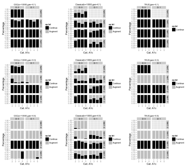
Figure 5: Simulation: The effect of the choice of $\gamma$ on the estimated optimal regime.

S5. The effect of the choice of tuning parameters on the estimated optimal regime.

In this section, we discuss the effect of the tuning parameters $(\alpha,\beta)$ on the estimated optimal treatment regime under the simulation scenario discussed in the manuscript. We generated 500 datasets of size 2000 and applied the proposed methods using various choices of tuning parameters:

• 1. $\alpha=\frac{\nu}{k\log(k)}$ and $\beta=\frac{\nu}{k}$ for $\nu=$0.050, 0.025, and 0.010

• 2. $\alpha=\frac{\nu}{k}$ and $\beta=\frac{\nu}{k^{3/4}}$ for $\nu=$0.050, 0.025, and 0.010

• 3. $\alpha=\frac{\nu}{k}$ and $\beta=\frac{\nu}{k^{1/3}}$ for $\nu=$0.050, and 0.010.

The parameter $\nu$ specifies the step size (increment size) for each choice of the tuning parameters. Figure 6 shows that as long as the step sizes are not very small, the stochastic minimization algorithm has a good performance. However, when the step sizes are small ($\nu=0.010$), the algorithm fails to converge to the true values because it cannot reach the true minimizers of the objective function. Table 1 presents the value of the objective function at the estimated $\hat{\theta}$ and the number of required iterations to converge ($K$) using different tuning parameters. The value of the objective function $M(\theta)$ for small $\nu$ is more than twice the value of $M(\theta)$ for larger values of $\nu$, which indicates the lack of convergence to the true minimizers. Based on this result, the first choice of tuning parameter, $\nu=0.05$, outperforms the other choices.

Figure 7 displays the effect of tuning parameters on standard errors. The vertical axis is the ratios of the standard errors obtained by different simulation scenarios over the standard error obtained by $\alpha=\frac{\nu}{k\log(k)}$ and $\beta=\frac{\nu}{k}$ and $\nu=0.050$. For example, the vertical axis in the first plot is

$$\frac{\text{S.D. of $\hat{\theta}$ when $\alpha=\frac{\nu}{k\log(k)}$, $\beta=\frac{\nu}{k}$ and $\nu=0.025$}}{\text{S.D. of $\hat{\theta}$ when $\alpha=\frac{\nu}{k\log(k)}$, $\beta=\frac{\nu}{k}$ and $\nu=0.050$}}.$$

Note that the reference S.D.s in the denominator includes the tuning parameter values used in the main simulation study in Section 4, which is shown to converge to the true values. In the first two rows, the ratios deviate more from one as the step size ($\nu$) gets smaller. This can be due to stoping the updates before converging to the minimizer of the objective function.

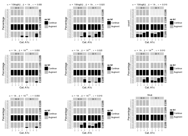
Figure 6: Simulation: The effect of the choice of tuning parameters on the estimated optimal regime.

Table 1: Simulation: The effect of the choice of tuning parameters on the estimated optimal regime.

	$\alpha=\frac{1}{k\log(k)}$, $\beta=\frac{1}{k}$			$\alpha=\frac{1}{k}$, $\beta=\frac{1}{k^{3/4}}$			$\alpha=\frac{1}{k}$, $\beta=\frac{1}{k^{1/3}}$
	$\nu=0.05$	$\nu=0.025$	$\nu=0.01$	$\nu=0.05$	$\nu=0.025$	$\nu=0.01$	$\nu=0.05$	$\nu=0.01$
$M(\theta)$	0.007	0.011	0.025	0.007	0.008	0.017	0.007	0.018
$K$	14.03	13.22	12.86	21.35	20.66	19.44	21.77	19.45

Figure 7: Simulation: The effect of the choice of tuning parameters on the standard errors.

References

• Bather (2000) Bather, J. (2000). Decision theory: an introduction to dynamic programming and sequential decisions, vol. 180. Wiley Hoboken, NJ.
• Bickel et al. (1993) Bickel, P. J., Klaassen, C. A. J., Ritov, Y. & Wellner, J. A. (1993). Efficient and adaptive estimation for semiparametric models. Johns Hopkins Series in the Mathematical Sciences. Baltimore, MD: Johns Hopkins University Press.
• Chakraborty et al. (2010) Chakraborty, B., Murphy, S. & Strecher, V. (2010). Inference for non-regular parameters in optimal dynamic treatment regimes. Statistical Methods in Medical Research 19, 317–343.
• Collins et al. (2004) Collins, L., Murphy, S. & Bierman, K. (2004). A conceptual framework for adaptive preventive interventions. Prevention Science 5, 185–196.
• Geyer (1994) Geyer, C. J. (1994). On the asymptotics of constrained m-estimation. The Annals of Statistics 2, 1993–2010.
• Goldberg & Kosorok (2011) Goldberg, Y. & Kosorok, M. R. (2011). Q-learning with censored data. Annals of Statistics 40, 529–560.
• Grundy et al. (2004) Grundy, S., Cleeman, J., Bairey Merz, C., Brewer Jr, H., Clark, L., Hunninghake, D., Pasternak, R., Smith Jr, S., Stone, N. et al. (2004). Implications of recent clinical trials for the national cholesterol education program adult treatment panel III guidelines. Journal of the American College of Cardiology 44, 720–732.
• Hunt (2008) Hunt, D. (2008). American diabetes association (ada) standards of medical care in diabetes 2008. Diabetes Care 31, S12–S54.
• Jordan (2002) Jordan, M. (2002). An introduction to probabilistic graphical models. University of California, Berkeley.
• Kahn et al. (2006) Kahn, S. E., Haffner, S. M., Heise, M. A., Herman, W. H., Holman, R. R., Jones, N. P., Kravitz, B. G., Lachin, J. M., O’Neill, M. C., Zinman, B. et al. (2006). Glycemic durability of rosiglitazone, metformin, or glyburide monotherapy. New England Journal of Medicine 355, 2427–2443.
• Laber et al. (2010) Laber, E., Qian, M., Lizotte, D. J. & Murphy, S. A. (2010). Statistical inference in dynamic treatment regimes. arXiv preprint arXiv:1006.5831 .
• Lavori & Dawson (2000) Lavori, P. & Dawson, R. (2000). A design for testing clinical strategies: biased adaptive within-subject randomization. Journal of the Royal Statistical Society: Series A (Statistics in Society) 163, 29–38.
• Maei et al. (2010) Maei, H., Szepesvári, C., Bhatnagar, S. & Sutton, R. (2010). Toward off-policy learning control with function approximation. Proc. ICML 2010 , 719–726.
• Mannor et al. (2007) Mannor, S., Simester, D., Sun, P. & Tsitsiklis, J. N. (2007). Bias and variance approximation in value function estimates. Management Science 53, 308–322.
• Moodie et al. (2007) Moodie, E., Richardson, T. & Stephens, D. (2007). Demystifying optimal dynamic treatment regimes. Biometrics 63, 447–455.
• Moody & Darken (1989) Moody, J. & Darken, C. J. (1989). Fast learning in networks of locally-tuned processing units. Neural computation 1, 281–294.
• Murphy (2003) Murphy, S. (2003). Optimal dynamic treatment regimes. Journal of the Royal Statistical Society: Series B (Statistical Methodology) 65, 331–355.
• Murphy et al. (2006) Murphy, S., Oslin, D., Rush, A. & Zhu, J. (2006). Methodological challenges in constructing effective treatment sequences for chronic psychiatric disorders. Neuropsychopharmacology 32, 257–262.
• Nahum-Shani et al. (2012) Nahum-Shani, I., Qian, M., Almirall, D., Pelham, W. E., Gnagy, B., Fabiano, G. A., Waxmonsky, J. G., Yu, J. & Murphy, S. A. (2012). Q-learning: A data analysis method for constructing adaptive interventions. Psychological Methods 17, 478.
• Neyman (1990) Neyman, J. (1990). On the application of probability theory to agricultural experiments. essay on principles. section 9. Translation of excerpts by D. Dabrowska and T. Speed. Statistical Science 6, 462–47.
• Parr et al. (2008) Parr, R., Li, L., Taylor, G., Painter-Wakefield, C. & Littman, M. L. (2008). An analysis of linear models, linear value-function approximation, and feature selection for reinforcement learning. In Proceedings of the 25th International Conference on Machine Learning.
• Poggio & Girosi (1990) Poggio, T. & Girosi, F. (1990). Networks for approximation and learning. Proceedings of the IEEE 78, 1481–1497.
• Robins (1986) Robins, J. (1986). A new approach to causal inference in mortality studies with a sustained exposure period–application to control of the healthy worker survivor effect. Mathematical Modelling 7, 1393–1512.
• Robins (1987) Robins, J. (1987). Addendum to a new approach to causal inference in mortality studies with a sustained exposure periodapplication to control of the healthy worker survivor effect. Computers & Mathematics With Applications 14, 923–945.
• Robins (2004) Robins, J. (2004). Optimal structural nested models for optimal sequential decisions. In Proceedings of the Second Seattle Symposium on Biostatistics. Springer: New York.
• Robins et al. (2008) Robins, J., Orellana, L. & Rotnitzky, A. (2008). Estimation and extrapolation of optimal treatment and testing strategies. Statistics in Medicine 27, 4678–4721.
• Robins (1994) Robins, J. M. (1994). Correcting for non-compliance in randomized trials using structural nested mean models. Communications in Statistics-Theory and Methods 23, 2379–2412.
• Robins (1997) Robins, J. M. (1997). Causal inference from complex longitudinal data. In Latent variable modeling and applications to causality. Springer, pp. 69–117.
• Rubin (1978) Rubin, D. B. (1978). Bayesian inference for causal effects: The role of randomization. The Annals of Statistics 6, 34–58.
• Schulte et al. (2014) Schulte, P. J., Tsiatis, A. A., Laber, E. B. & Davidian, M. (2014). Q-and A-learning methods for estimating optimal dynamic treatment regimes. Statistical Science in press.
• Si (2004) Si, J. (2004). Handbook of learning and approximate dynamic programming, vol. 2. Wiley-IEEE Press.
• Simester et al. (2006) Simester, D. I., Sun, P. & Tsitsiklis, J. N. (2006). Dynamic catalog mailing policies. Management Science 52, 683–696.
• Sutton & Barto (1998) Sutton, R. & Barto, A. (1998). Reinforcement learning: An introduction, vol. 28. Cambridge Univ Press.
• Sutton et al. (2009a) Sutton, R., Maei, H., Precup, D., Bhatnagar, S., Silver, D., Szepesvári, C. & Wiewiora, E. (2009a). Fast gradient-descent methods for temporal-difference learning with linear function approximation. In Proceedings of the 26th annual International Conference on Machine Learning. ACM.
• Sutton et al. (2009b) Sutton, R., Szepesvári, C. & Maei, H. (2009b). A convergent o (n) algorithm for off-policy temporal-difference learning with linear function approximation. Advances in Neural Information Processing Systems 21 .
• Tang & Kosorok (2012) Tang, Y. & Kosorok, M. R. (2012). Developing adaptive personalized therapy for cystic fibrosis using reinforcement learning. Tech. rep., The University of North Carolina at Chapel Hill.
• Timbie et al. (2010) Timbie, J., Hayward, R. & Vijan, S. (2010). Diminishing efficacy of combination therapy, response-heterogeneity, and treatment intolerance limit the attainability of tight risk factor control in patients with diabetes. Health Services Research 45, 437–456.
• Van Der Vaart & Wellner (1996) Van Der Vaart, A. & Wellner, J. (1996). Weak convergence and empirical processes. Springer Verlag.
• Vapnik et al. (1997) Vapnik, V., Golowich, S. E. & Smola, A. (1997). Support vector method for function approximation, regression estimation, and signal processing. Advances in neural information processing systems , 281–287.
• Zhang et al. (2012) Zhang, B., Tsiatis, A. A., Laber, E. B. & Davidian, M. (2012). A robust method for estimating optimal treatment regimes. Biometrics 68, 1010–1018.
• Zhang et al. (2013) Zhang, B., Tsiatis, A. A., Laber, E. B. & Davidian, M. (2013). Robust estimation of optimal dynamic treatment regimes for sequential treatment decisions. Biometrika 100, 1–14.
• Zhao et al. (2009) Zhao, Y., Kosorok, M. R. & Zeng, D. (2009). Reinforcement learning design for cancer clinical trials. Statistics in medicine 28, 3294–3315.
• Zhao et al. (2011) Zhao, Y., Zeng, D., Socinski, M. A. & Kosorok, M. R. (2011). Reinforcement learning strategies for clinical trials in nonsmall cell lung cancer. Biometrics 67, 1422–1433.