Large-Spin and Large-Winding Expansions
of Giant Magnons and Single Spikes

Emmanuel Floratos and Georgios Linardopoulos111E-mails: mflorato@phys.uoa.gr, glinard@inp.demokritos.gr.
Department of Physics, National and Kapodistrian University of Athens,
Zografou Campus, 157 84, Athens, Greece
Institute of Nuclear and Particle Physics, N.C.S.R., ”Demokritos”,
153 10, Agia Paraskevi, Greece
Abstract

We generalize the method of our recent paper on the large-spin expansions of Gubser-Klebanov-Polyakov (GKP) strings to the large-spin and large-winding expansions of finite-size giant magnons and finite-size single spikes. By expressing the energies of long open strings in $\mathbb{R}\times\text{S}^{2}$ in terms of Lambert’s W-function, we compute the leading, subleading and next-to-subleading series of classical exponential corrections to the dispersion relations of Hofman-Maldacena giant magnons and infinite-winding single spikes. We also compute the corresponding expansions in the doubled regions of giant magnons and single spikes that are respectively obtained when their angular and linear velocities become smaller or greater than unity.

1 Introduction and Motivation

The exact computation of the full spectrum of the AdS/CFT correspondence [1, 2, 3] and the comparison of the scaling dimensions of local operators of planar $\mathcal{N}=4$ super Yang-Mills (SYM) theory to the energies of free string states of type IIB superstring theory in AdS${}_{5}\times\text{S}^{5}$, is one first step towards the determination of the precise relationship between these two theories (that are typically treated as identical in AdS/CFT’s strongest formulations). It is therefore very important to identify and study the elementary excitations that string theory in AdS${}_{5}\times\text{S}^{5}$ and $\mathcal{N}=4$ SYM theory share and are the fundamental building blocks out of which the corresponding spectra may be built.
Giant magnons (GMs) are open, single-spin strings that rotate in $\mathbb{R}\times\text{S}^{2}\subset\text{AdS}_{5}\times\text{S}^{5}$. They were found in 2006 by Hofman and Maldacena (HM) [4] and were identified as the string theory duals of magnon excitations of $\mathcal{N}=4$ SYM. Giant magnons are elementary excitations of the IIB Green-Schwarz superstring on AdS${}_{5}\times\text{S}^{5}$, out of which closed strings and multi-soliton solutions may be formed. The energy-spin relation of a single giant magnon of angular extent $\Delta\varphi$ on a 2-sphere of radius $R$ is:

E - J = λπ—sinΔφ2—,  J = ∞, λR2α→∞, (1.1)E - J = λπ—sinΔφ2—,  J = ∞, λsuperscriptR2α→∞, (1.1)\halign to=0.0pt{\relax\global\advance\@IEEEeqncolcnt by 1\relax\begingroup\csname @IEEEeqnarraycolPREc\endcsname#\relax\relax\relax\relax\relax\relax\relax\relax\relax\relax\csname @IEEEeqnarraycolPOSTc\endcsname\relax\relax\relax\relax\relax\relax\relax\relax\relax\relax\endgroup&\global\advance\@IEEEeqncolcnt by 1\relax\bgroup#\egroup&\global\advance\@IEEEeqncolcnt by 1\relax\hbox to\z@\bgroup\hss#\egroup\cr\hfil$\displaystyle E - J = \frac{\sqrt{\lambda}}{\pi} \, \left|\sin\frac{\Delta\varphi}{2}\right|, \quad J = \infty, \ \sqrt{\lambda} = \frac{R^{2}}{\alpha'} \rightarrow\infty, $\hfil&{\vrule width=0.0pt,height=0.0pt,depth=0.0pt}&0.0pt{\hss{\normalcolor(1.1)}}\cr}

where $\Delta\varphi=p$ is the giant magnon’s momentum. Superimposing two giant magnons of maximum angular extent $\Delta\varphi=\pi$ gives the Gubser-Klebanov-Polyakov (GKP) closed and folded string that rotates on S2 [5], the dispersion relation of which is

E - J = 2λπ,  J = ∞, λ→∞. (1.2)E - J = 2λπ,  J = ∞, λ→∞. (1.2)\halign to=0.0pt{\relax\global\advance\@IEEEeqncolcnt by 1\relax\begingroup\csname @IEEEeqnarraycolPREc\endcsname#\relax\relax\relax\relax\relax\relax\relax\relax\relax\relax\csname @IEEEeqnarraycolPOSTc\endcsname\relax\relax\relax\relax\relax\relax\relax\relax\relax\relax\endgroup&\global\advance\@IEEEeqncolcnt by 1\relax\bgroup#\egroup&\global\advance\@IEEEeqncolcnt by 1\relax\hbox to\z@\bgroup\hss#\egroup\cr\hfil$\displaystyle E - J = \frac{2\sqrt{\lambda}}{\pi}, \quad J = \infty, \ \lambda\rightarrow\infty. $\hfil&{\vrule width=0.0pt,height=0.0pt,depth=0.0pt}&0.0pt{\hss{\normalcolor(1.2)}}\cr}

According to the AdS/CFT correspondence, the energy $E$ of a string state in AdS${}_{5}\times\text{S}^{5}$ should equal the scaling dimension $\Delta$ of its dual $\mathcal{N}=4$ SYM operator. Despite the finiteness of $\mathcal{N}=4$ SYM, its operators typically get renormalized and they thus acquire anomalous dimensions $\gamma$, which are the eigenvalues of the gauge theory dilatation operator. The anomalous dimensions may also be found at strong coupling by calculating the energy of their dual strings. Although there exists no systematic way by which to assign a certain gauge theory operator to its dual string state, many such heuristic identifications are known. The above GKP string that rotates inside $\mathbb{R}\times\text{S}^{2}$ for example is dual to the operator $\text{Tr}\left[\mathcal{X}\mathcal{Z}^{m}\mathcal{X}\mathcal{Z}^{J-m}\right]+\ldots$ of $\mathcal{N}=4$ SYM.
It has been known for quite some time that the one-loop dilatation operator of $\mathcal{N}=4$ SYM theory [6] has the form of an integrable $\mathfrak{psu}\left(2,2|4\right)$ spin chain Hamiltonian, which can be diagonalized by means of the Bethe ansatz (BA) [7, 8]. An all-loop asymptotic Bethe ansatz (ABA) for the $\mathfrak{su}\left(2\right)$ sector of $\mathcal{N}=4$ SYM(333The compact $\mathfrak{su}\left(2\right)$ sector of $\mathcal{N}=4$ super Yang-Mills consists of the single-trace operators $\text{Tr}\left[\mathcal{Z}^{J}\mathcal{X}^{M}\right]$, where $\mathcal{X},\ \mathcal{Y},\ \mathcal{Z}$ are the three complex scalar fields of $\mathcal{N}=4$ SYM, composed out of the six real scalars $\Phi$ of the theory. The $\mathfrak{su}\left(2\right)$ sector is dual to (closed) strings that rotate in $\mathbb{R}\times\text{S}^{3}\subset\text{AdS}_{5}\times\text{S}^{5}$ and its one-loop dilatation operator is given by the Hamiltonian of the ferromagnetic XXX1/2 Heisenberg spin chain.) has been proposed by Beisert, Dippel and Staudacher (BDS) [9]. The BDS energy for single magnon states (the elementary spin chain excitations that are dual to GMs) in a spin chain of length $J+1$ is:

ϵ≡E - J = 1 + λπ2sin2(p2)λ= gYM2N, (1.3)subscriptϵ≡E - J = 1 + λsuperscriptπ2superscriptsin2p2superscriptsubscriptλ= gYM2N, (1.3)\halign to=0.0pt{\relax\global\advance\@IEEEeqncolcnt by 1\relax\begingroup\csname @IEEEeqnarraycolPREc\endcsname#\relax\relax\relax\relax\relax\relax\relax\relax\relax\relax\csname @IEEEeqnarraycolPOSTc\endcsname\relax\relax\relax\relax\relax\relax\relax\relax\relax\relax\endgroup&\global\advance\@IEEEeqncolcnt by 1\relax\bgroup#\egroup&\global\advance\@IEEEeqncolcnt by 1\relax\hbox to\z@\bgroup\hss#\egroup\cr\hfil$\displaystyle\epsilon_{\infty}\equiv E - J = \sqrt{1 + \frac{\lambda}{\pi^{2}}\sin^{2}\left(\frac{p}{2}\right)}, \quad\lambda= g_{\text{YM}}^{2} N, $\hfil&{\vrule width=0.0pt,height=0.0pt,depth=0.0pt}&0.0pt{\hss{\normalcolor(1.3)}}\cr}

where $p$ is the magnon’s momentum. At strong ’t Hooft coupling ($\lambda\rightarrow\infty$) (1) gives (1) to lowest order and the first quantum correction (aka one-loop shift) vanishes. At weak coupling, the one-loop magnon energy is recovered to lowest order in $\lambda$:

E - J = 1 + λ2π2sin2(p2)+ … , λ→0. (1.4)E - J = 1 + λsuperscript2π2superscriptsin2p2+ … , λ→0. (1.4)\halign to=0.0pt{\relax\global\advance\@IEEEeqncolcnt by 1\relax\begingroup\csname @IEEEeqnarraycolPREc\endcsname#\relax\relax\relax\relax\relax\relax\relax\relax\relax\relax\csname @IEEEeqnarraycolPOSTc\endcsname\relax\relax\relax\relax\relax\relax\relax\relax\relax\relax\endgroup&\global\advance\@IEEEeqncolcnt by 1\relax\bgroup#\egroup&\global\advance\@IEEEeqncolcnt by 1\relax\hbox to\z@\bgroup\hss#\egroup\cr\hfil$\displaystyle E - J = 1 + \frac{\lambda}{2\pi^{2}}\sin^{2}\left(\frac{p}{2}\right) + \ldots\,, \quad\lambda\rightarrow 0. $\hfil&{\vrule width=0.0pt,height=0.0pt,depth=0.0pt}&0.0pt{\hss{\normalcolor(1.4)}}\cr}

A very important discovery made by Beisert in 2005 [10] is that the dispersion relation (1) can be determined uniquely from the corresponding symmetry algebra, the centrally extended $\mathfrak{su}\left(2|2\right)\oplus\mathfrak{su}\left(2|2\right)\subset\mathfrak{psu}\left(2,2|4\right)$.
The asymptotic Bethe ansatz can lead to the correct form of the anomalous dimensions only when the length $L$ of the spin chain is infinite or larger than the loop order $L$. At and above this critical loop-order $L$, the range of the spin chain interactions exceeds the length of the spin chain (virtual particles start circulating around the spin chain) and wrapping corrections have to be taken into account. The inefficiency of the ABA beyond the critical loop-order has been noted in both the gauge and the string theory [11, 12]. Conversely, the wrapping effects that appear at the critical loop-order have the form of exponentially small corrections to the anomalous dimensions, as noted in [13]. The thermodynamic Bethe ansatz (TBA), the Y-system and the quantum spectral curve (QSC) [14, 15, 16] are three proposals that correctly account for the wrapping corrections.
On the string theory side, one equivalently calculates classical and quantum exponential corrections to the giant magnon dispersion relation (1), the general form of which is:

ϵ(p)ϵλδϵclδϵ1-loop1λδϵ2-loop+ …, (1.5)ϵpsubscriptϵλsubscriptδϵclsubscriptδϵ1-loop1λsubscriptδϵ2-loop+ …, missing-subexpression(1.5)\halign to=0.0pt{\relax\global\advance\@IEEEeqncolcnt by 1\relax\begingroup\csname @IEEEeqnarraycolPREl\endcsname#\relax\relax\relax\relax\relax\relax\relax\relax\relax\relax\csname @IEEEeqnarraycolPOSTl\endcsname\relax\relax\relax\relax\relax\relax\relax\relax\relax\relax\endgroup&\relax\global\advance\@IEEEeqncolcnt by 1\relax\begingroup\csname @IEEEeqnarraycolPREl\endcsname#\relax\relax\relax\relax\relax\relax\relax\relax\relax\relax\csname @IEEEeqnarraycolPOSTl\endcsname\relax\relax\relax\relax\relax\relax\relax\relax\relax\relax\endgroup&\global\advance\@IEEEeqncolcnt by 1\relax\bgroup#\egroup&\global\advance\@IEEEeqncolcnt by 1\relax\hbox to\z@\bgroup\hss#\egroup\cr$\displaystyle\epsilon\left(p\right) = \epsilon_{\infty}+ \sqrt{\lambda}\,\delta\epsilon_{\text{cl}} + \delta\epsilon_{\text{1-loop}} + \frac{1}{\sqrt{\lambda}}\,\delta\epsilon_{\text{2-loop}} + \ldots, $\hfil&$\displaystyle$\hfil&{\vrule width=0.0pt,height=0.0pt,depth=0.0pt}&0.0pt{\hss{\normalcolor(1.5)}}\cr}

where $\epsilon\left(p\right)\equiv E-J$. The first few terms of the classical finite-size expansion $\delta\epsilon_{\text{cl}}$ were first derived by Arutyunov, Frolov and Zamaklar (AFZ) in [17]:

δϵcl= - 4πsinp2{sin2p2eL[8J2cos2p2+ 4sinp2(3cosp + 2)J + (1.6)+ sin2p2(6cosp + 7)]e- 2L+ …}J ≡πJλL ≡2J cscp2+ 2. (1.7)subscriptδϵcl= - 4πsinp2{superscriptsin2p2superscripteLsuperscript[8J2superscriptcos2p2+ 4sinp23cosp + 2J + (1.6)missing-subexpressionsuperscript+ sin2p26cosp + 7superscript]e- 2L+ …}J ≡πJλL ≡2J cscp2+ 2. (1.7)\halign to=0.0pt{\relax\global\advance\@IEEEeqncolcnt by 1\relax\begingroup\csname @IEEEeqnarraycolPREl\endcsname#\relax\relax\relax\relax\relax\relax\relax\relax\relax\relax\csname @IEEEeqnarraycolPOSTl\endcsname\relax\relax\relax\relax\relax\relax\relax\relax\relax\relax\endgroup&\relax\global\advance\@IEEEeqncolcnt by 1\relax\begingroup\csname @IEEEeqnarraycolPREl\endcsname#\relax\relax\relax\relax\relax\relax\relax\relax\relax\relax\csname @IEEEeqnarraycolPOSTl\endcsname\relax\relax\relax\relax\relax\relax\relax\relax\relax\relax\endgroup&\global\advance\@IEEEeqncolcnt by 1\relax\bgroup#\egroup&\global\advance\@IEEEeqncolcnt by 1\relax\hbox to\z@\bgroup\hss#\egroup\cr$\displaystyle\delta\epsilon_{\text{cl}} = - \frac{4}{\pi} \, \sin\frac{p}{2} \, \Bigg{\{}$\hfil&$\displaystyle\sin^{2}\frac{p}{2}\,e^{- \mathcal{L}} + \bigg{[}8\mathcal{J}^{2}\cos^{2}\frac{p}{2} + 4\sin\frac{p}{2}\left(3\cos p + 2\right)\mathcal{J} + $\hfil&{{}\vrule width=0.0pt,height=0.0pt,depth=0.0pt}&0.0pt{\hss{\normalcolor(1.6)}}\cr\penalty 0\vskip 3.0pt\vskip 6.0pt\cr$\displaystyle$\hfil&$\displaystyle+ \sin^{2}\frac{p}{2}\left(6\cos p + 7\right)\bigg{]}e^{- 2\mathcal{L}} + \ldots\Bigg{\}}, \quad\mathcal{J} \equiv\frac{\pi J}{\sqrt{\lambda}}, \quad\mathcal{L} \equiv 2\mathcal{J} \csc\frac{p}{2} + 2. \qquad $\hfil&{\vrule width=0.0pt,height=0.0pt,depth=0.0pt}&0.0pt{\hss{\normalcolor(1.7)}}\cr}

Astolfi, Forini, Grignani and Semenoff have proven in [18] that the spectrum of finite-size giant magnons in the uniform light-cone gauge is completely independent of the corresponding gauge parameter. From (1) the structure of the classical finite-size corrections $\delta\epsilon_{\text{cl}}$ may be deduced:444The authors wish to thank an anonymous referee for his/her valuable suggestions regarding the general form of $\delta\epsilon_{\text{cl}}$.

δϵcl1π⋅∑n = 1m = 02n - 2Anm(p)J2n - m - 2e-2n(Jcscp2+ 1)(1.8) = 1π⋅∑m = 0J-m - 2{n = ⌊m2+ 1⌋Anm(p)J2ne-2n(Jcscp2+ 1)}(1.9)subscriptδϵcl1πsuperscriptsubscript⋅∑n = 1superscriptsubscriptm = 02n - 2subscriptAnmpsuperscriptJ2n - m - 2superscripte-2nJcscp2+ 1(1.8)missing-subexpression = 1πsuperscriptsubscript⋅∑m = 0superscriptJ-m - 2superscriptsubscriptn = ⌊m2+ 1⌋subscriptAnmpsuperscriptJ2nsuperscripte-2nJcscp2+ 1(1.9)\halign to=0.0pt{\relax\global\advance\@IEEEeqncolcnt by 1\relax\begingroup\csname @IEEEeqnarraycolPREl\endcsname#\relax\relax\relax\relax\relax\relax\relax\relax\relax\relax\csname @IEEEeqnarraycolPOSTl\endcsname\relax\relax\relax\relax\relax\relax\relax\relax\relax\relax\endgroup&\relax\global\advance\@IEEEeqncolcnt by 1\relax\begingroup\csname @IEEEeqnarraycolPREl\endcsname#\relax\relax\relax\relax\relax\relax\relax\relax\relax\relax\csname @IEEEeqnarraycolPOSTl\endcsname\relax\relax\relax\relax\relax\relax\relax\relax\relax\relax\endgroup&\global\advance\@IEEEeqncolcnt by 1\relax\bgroup#\egroup&\global\advance\@IEEEeqncolcnt by 1\relax\hbox to\z@\bgroup\hss#\egroup\cr$\displaystyle\delta\epsilon_{\text{cl}} $\hfil&$\displaystyle= \frac{1}{\pi} \cdot\sum_{n = 1}^{\infty} \sum_{m = 0}^{2n - 2} \mathcal{A}_{nm}\left(p\right)\mathcal{J}^{2n - m - 2} e^{-2n\left(\mathcal{J}\csc\frac{p}{2} + 1\right)} = $\hfil&{{}\vrule width=0.0pt,height=0.0pt,depth=0.0pt}&0.0pt{\hss{\normalcolor(1.8)}}\cr\penalty 0\vskip 3.0pt\vskip 6.0pt\cr$\displaystyle$\hfil&$\displaystyle\hskip 56.9055pt = \frac{1}{\pi} \cdot\sum_{m = 0}^{\infty} \mathcal{J}^{-m - 2} \left\{ \sum_{n = \lfloor\frac{m}{2} + 1\rfloor}^{\infty} \mathcal{A}_{nm}\left(p\right)\mathcal{J}^{2n} e^{-2n\left(\mathcal{J}\csc\frac{p}{2} + 1\right)}\right\}. \qquad $\hfil&{\vrule width=0.0pt,height=0.0pt,depth=0.0pt}&0.0pt{\hss{\normalcolor(1.9)}}\cr}

Formula (1) contains the terms $\mathcal{A}_{10}$, $\mathcal{A}_{20}$, $\mathcal{A}_{21}$, $\mathcal{A}_{22}$. Of course, many more classical terms may be rather easily obtained by a direct computation with e.g. $\mathsf{Mathematica}$ (cf. appendix B). Klose and McLoughlin [19] have obtained the terms $\mathcal{A}_{n0}$ ($1\leq n\leq 6$) of the series (1):

δϵcl= - 4πsin3p2e-L[+ 2 L2cos2p2e-L+ 8 L4cos4p2e-2L1283L6cos6p2e-3L(1.10)8003L8cos8p2e-4L92165L10cos10p2e-5L+ …](1.11)subscriptδϵcl= - 4πsuperscriptsin3p2superscripte-L[superscript+ 2 L2superscriptcos2p2superscripte-Lsuperscript+ 8 L4superscriptcos4p2superscripte-2L1283superscriptL6superscriptcos6p2superscripte-3L(1.10)missing-subexpression8003superscriptL8superscriptcos8p2superscripte-4L92165superscriptL10superscriptcos10p2superscripte-5L+ …](1.11)\halign to=0.0pt{\relax\global\advance\@IEEEeqncolcnt by 1\relax\begingroup\csname @IEEEeqnarraycolPREl\endcsname#\relax\relax\relax\relax\relax\relax\relax\relax\relax\relax\csname @IEEEeqnarraycolPOSTl\endcsname\relax\relax\relax\relax\relax\relax\relax\relax\relax\relax\endgroup&\relax\global\advance\@IEEEeqncolcnt by 1\relax\begingroup\csname @IEEEeqnarraycolPREl\endcsname#\relax\relax\relax\relax\relax\relax\relax\relax\relax\relax\csname @IEEEeqnarraycolPOSTl\endcsname\relax\relax\relax\relax\relax\relax\relax\relax\relax\relax\endgroup&\global\advance\@IEEEeqncolcnt by 1\relax\bgroup#\egroup&\global\advance\@IEEEeqncolcnt by 1\relax\hbox to\z@\bgroup\hss#\egroup\cr$\displaystyle\delta\epsilon_{\text{cl}} = - \frac{4}{\pi} \, \sin^{3}\frac{p}{2} \, e^{-\mathcal{L}}\bigg{[}1 $\hfil&$\displaystyle+ 2\,\mathcal{L}^{2}\,\cos^{2}\frac{p}{2}\,e^{-\mathcal{L}} + 8\,\mathcal{L}^{4}\,\cos^{4}\frac{p}{2}\,e^{-2\mathcal{L}} + \frac{128}{3}\,\mathcal{L}^{6}\,\cos^{6}\frac{p}{2}\,e^{-3\mathcal{L}} + $\hfil&{{}\vrule width=0.0pt,height=0.0pt,depth=0.0pt}&0.0pt{\hss{\normalcolor(1.10)}}\cr\penalty 0\vskip 3.0pt\vskip 6.0pt\cr$\displaystyle$\hfil&$\displaystyle+ \frac{800}{3}\,\mathcal{L}^{8}\,\cos^{8}\frac{p}{2}\,e^{-4\mathcal{L}} + \frac{9216}{5}\,\mathcal{L}^{10}\,\cos^{10}\frac{p}{2}\,e^{-5\mathcal{L}} + \ldots\bigg{]}. \qquad $\hfil&{\vrule width=0.0pt,height=0.0pt,depth=0.0pt}&0.0pt{\hss{\normalcolor(1.11)}}\cr}

The leading term $\mathcal{A}_{10}$ of (1)–(1) has also been obtained by the algebraic curve method in [20], as well as by applying the Lüscher-Klassen-Melzer (LKM) formulae [21, 22] at strong coupling [23, 24, 25].
At the quantum level it has explicitly been shown in [26, 27] that, in accordance with (1), the infinite-volume one-loop shift vanishes:

δϵ1-loop= 0,  J = ∞, λ→∞. (1.12)subscriptδϵ1-loop= 0,  J = ∞, λ→∞. (1.12)\halign to=0.0pt{\relax\global\advance\@IEEEeqncolcnt by 1\relax\begingroup\csname @IEEEeqnarraycolPREc\endcsname#\relax\relax\relax\relax\relax\relax\relax\relax\relax\relax\csname @IEEEeqnarraycolPOSTc\endcsname\relax\relax\relax\relax\relax\relax\relax\relax\relax\relax\endgroup&\global\advance\@IEEEeqncolcnt by 1\relax\bgroup#\egroup&\global\advance\@IEEEeqncolcnt by 1\relax\hbox to\z@\bgroup\hss#\egroup\cr\hfil$\displaystyle\delta\epsilon_{\text{1-loop}} = 0, \quad J = \infty, \ \lambda\rightarrow\infty. $\hfil&{\vrule width=0.0pt,height=0.0pt,depth=0.0pt}&0.0pt{\hss{\normalcolor(1.12)}}\cr}

At finite volume the calculation of loop shifts proceeds either via the algebraic curve method [25] or by calculating the Lüscher-F and $\mu$-terms [24]. The general form of the one-loop shift is:

δϵ1-loop= a1,0e-2D+ ∑n=0m=1an,me-2 n D - mL,  D≡J + sinp2(1.13)subscriptδϵ1-loopsubscript= a1,0superscripte-2Dsuperscriptsubscript+ ∑n=0m=1subscriptan,msuperscripte-2 n D - mL,  D≡J + sinp2(1.13)\halign to=0.0pt{\relax\global\advance\@IEEEeqncolcnt by 1\relax\begingroup\csname @IEEEeqnarraycolPREc\endcsname#\relax\relax\relax\relax\relax\relax\relax\relax\relax\relax\csname @IEEEeqnarraycolPOSTc\endcsname\relax\relax\relax\relax\relax\relax\relax\relax\relax\relax\endgroup&\global\advance\@IEEEeqncolcnt by 1\relax\bgroup#\egroup&\global\advance\@IEEEeqncolcnt by 1\relax\hbox to\z@\bgroup\hss#\egroup\cr\hfil$\displaystyle\delta\epsilon_{\text{1-loop}} = a_{1,0} \, e^{-2D} + \sum_{\begin{subarray}{c}n=0\\ m=1\end{subarray}}^{\infty}a_{n,m} e^{-2 n D - m\mathcal{L}}, \quad D\equiv\mathcal{J} + \sin\frac{p}{2}. $\hfil&{\vrule width=0.0pt,height=0.0pt,depth=0.0pt}&0.0pt{\hss{\normalcolor(1.13)}}\cr}

Formulas which allow the calculation of $a_{n,0}$ and $a_{1,m}$ in the above expansion have been given in [25, 28]. The first term $a_{1,0}$ is given by:

a1,01D8sin2p/4(sinp/2 - 1)[1 - 7 + 4sinp -4cosp + sinp/216(sinp/2 - 1)1D+ O(1D2)](1.14)subscripta1,01Dsuperscript8sin2p/4sinp/2 - 1delimited-[]1 - 7 + 4sinp -4cosp + sinp/216sinp/2 - 11D+ O1superscriptD2(1.14)\halign to=0.0pt{\relax\global\advance\@IEEEeqncolcnt by 1\relax\begingroup\csname @IEEEeqnarraycolPREc\endcsname#\relax\relax\relax\relax\relax\relax\relax\relax\relax\relax\csname @IEEEeqnarraycolPOSTc\endcsname\relax\relax\relax\relax\relax\relax\relax\relax\relax\relax\endgroup&\global\advance\@IEEEeqncolcnt by 1\relax\bgroup#\egroup&\global\advance\@IEEEeqncolcnt by 1\relax\hbox to\z@\bgroup\hss#\egroup\cr\hfil$\displaystyle a_{1,0} = \frac{1}{\sqrt{D}}\frac{8\sin^{2} p/4}{\left(\sin p/2 - 1\right)}\left[1 - \frac{7 + 4\sin p -4\cos p + \sin p/2}{16\left(\sin p/2 - 1\right)}\cdot\frac{1}{D} + O\left(\frac{1}{D^{2}}\right)\right]. $\hfil&{\vrule width=0.0pt,height=0.0pt,depth=0.0pt}&0.0pt{\hss{\normalcolor(1.14)}}\cr}

Other generalizations of the GM include giant magnons in $\beta$-deformed backgrounds [29, 30], TsT-transformed AdS${}_{5}\times\text{S}^{5}$ [31, 32] and AdS${}_{4}/\text{CFT}_{3}$ [33, 34].
From the string point of view, the HM giant magnon is a close relative of yet another string sigma model solution on the 2-sphere, the single spike (SS) [35, 36]. In the conformal gauge, one may obtain the single spike from the HM ansatz by interchanging the world-sheet coordinates on the 2-sphere, i.e. $\tau\leftrightarrow\sigma$.555Note that this transformation should not affect the choice of the temporal gauge, $t=\tau$. The corresponding dispersion relation is ($\Delta\varphi=p$, $T=\sqrt{\lambda}/2\pi$):

E - TΔφλπarcsin(πJλ),  p = ∞, λ→∞, (1.15)E - TΔφλπarcsinπJλ,  p = ∞, λ→∞, (1.15)\halign to=0.0pt{\relax\global\advance\@IEEEeqncolcnt by 1\relax\begingroup\csname @IEEEeqnarraycolPREc\endcsname#\relax\relax\relax\relax\relax\relax\relax\relax\relax\relax\csname @IEEEeqnarraycolPOSTc\endcsname\relax\relax\relax\relax\relax\relax\relax\relax\relax\relax\endgroup&\global\advance\@IEEEeqncolcnt by 1\relax\bgroup#\egroup&\global\advance\@IEEEeqncolcnt by 1\relax\hbox to\z@\bgroup\hss#\egroup\cr\hfil$\displaystyle E - T\Delta\varphi= \frac{\sqrt{\lambda}}{\pi} \, \arcsin\left(\frac{\pi J}{\sqrt{\lambda}}\right) , \quad p = \infty, \ \lambda\rightarrow\infty, $\hfil&{\vrule width=0.0pt,height=0.0pt,depth=0.0pt}&0.0pt{\hss{\normalcolor(1.15)}}\cr}

which can be transformed back to the dispersion relation of the giant magnon (1), by making the transformations $\pi E/\sqrt{\lambda}-\Delta\varphi/2\mapsto p/2$ and $J\mapsto E-J$. It has been claimed in [37] that the $\tau\leftrightarrow\sigma$ transform carries us from large-spin strings in $\mathbb{R}\times\text{S}^{2}$ to large-winding ones, and from the holomorphic sector of $\mathcal{N}=4$ SYM to its non-holomorphic sector. Furthermore, just as the GMs are the string theory duals of magnons, the elementary excitations above the ferromagnetic ground state $\text{Tr}\mathcal{Z}^{J}$ of the XXX1/2 spin chain, the SSs are the string theory duals of the corresponding elementary excitations above the anti-ferromagnetic ground state $\text{Tr}\mathcal{S}^{L/2}$ of an SO$\left(6\right)$ SYM spin chain.666Applying the $\tau\leftrightarrow\sigma$ transform to the string theory dual of the BPS vacuum $\text{Tr}\mathcal{Z}^{J}$, which is a point-like string moving around the equator of S2, we obtain the string theory dual of the anti-ferromagnetic vacuum $\text{Tr}\mathcal{S}^{L/2}+\ldots$, a string at rest that is wound around the equator of S2 and is called the hoop string. According to [37], $\mathcal{S}\sim\mathcal{X}\overline{\mathcal{X}}+\mathcal{Y}\overline{\mathcal{Y}}+\mathcal{Z}\overline{\mathcal{Z}}$ is an SO$\left(6\right)$ singlet composite operator of $\mathcal{N}=4$ SYM.
Being located near the top of the string spectrum, both the hoop string (the string theory dual of the anti-ferromagnetic vacuum) and single spikes are expected to be unstable [38]. They might however be stabilized in many ways, e.g. by adding extra angular momenta. Finite momentum effects for single spikes have been considered in [39]. The following result,

E - TΔφλπ[q2+ 4sin2q2tanq2⋅e-(q + Δφ)⋅cotq2],  q ≡2arcsin(πJλ)(1.16)E - TΔφλπ[q2superscript+ 4sin2q2tanq2superscript⋅e-q + Δφ⋅cotq2],  q ≡2arcsinπJλ(1.16)\halign to=0.0pt{\relax\global\advance\@IEEEeqncolcnt by 1\relax\begingroup\csname @IEEEeqnarraycolPREc\endcsname#\relax\relax\relax\relax\relax\relax\relax\relax\relax\relax\csname @IEEEeqnarraycolPOSTc\endcsname\relax\relax\relax\relax\relax\relax\relax\relax\relax\relax\endgroup&\global\advance\@IEEEeqncolcnt by 1\relax\bgroup#\egroup&\global\advance\@IEEEeqncolcnt by 1\relax\hbox to\z@\bgroup\hss#\egroup\cr\hfil$\displaystyle E - T\Delta\varphi= \frac{\sqrt{\lambda}}{\pi}\Bigg{[}\frac{q}{2} + 4\sin^{2}\frac{q}{2}\tan\frac{q}{2}\cdot e^{-\left(q + \Delta\varphi\right)\cdot\cot\frac{q}{2}}\Bigg{]}, \quad q \equiv 2\arcsin\left(\frac{\pi J}{\sqrt{\lambda}}\right), $\hfil&{\vrule width=0.0pt,height=0.0pt,depth=0.0pt}&0.0pt{\hss{\normalcolor(1.16)}}\cr}

contains the first, leading finite-momentum correction. The general structure of the dispersion relation of classical single spikes at finite volume is similar to the one for giant magnons, albeit with the roles of $p$ and $\mathcal{J}$ interchanged:

E - p2clasq2+ ∑n = 1m = 02n - 2A^nm(q)p2n - m - 2e-n(q + p)cotq2(1.17)E - p2subscriptclasq2superscriptsubscript+ ∑n = 1superscriptsubscriptm = 02n - 2subscript^Anmqsuperscriptp2n - m - 2superscripte-nq + pcotq2(1.17)\halign to=0.0pt{\relax\global\advance\@IEEEeqncolcnt by 1\relax\begingroup\csname @IEEEeqnarraycolPREl\endcsname#\relax\relax\relax\relax\relax\relax\relax\relax\relax\relax\csname @IEEEeqnarraycolPOSTl\endcsname\relax\relax\relax\relax\relax\relax\relax\relax\relax\relax\endgroup&\relax\global\advance\@IEEEeqncolcnt by 1\relax\begingroup\csname @IEEEeqnarraycolPREl\endcsname#\relax\relax\relax\relax\relax\relax\relax\relax\relax\relax\csname @IEEEeqnarraycolPOSTl\endcsname\relax\relax\relax\relax\relax\relax\relax\relax\relax\relax\endgroup&\global\advance\@IEEEeqncolcnt by 1\relax\bgroup#\egroup&\global\advance\@IEEEeqncolcnt by 1\relax\hbox to\z@\bgroup\hss#\egroup\cr$\displaystyle\mathcal{E} - \frac{p}{2}\Bigg{|}_{\text{clas}} $\hfil&$\displaystyle= \frac{q}{2} + \sum_{n = 1}^{\infty} \sum_{m = 0}^{2n - 2} \hat{\mathcal{A}}_{nm}\left(q\right) p^{2n - m - 2} e^{-n\left(q + p\right)\cot\frac{q}{2}}\,. \qquad $\hfil&{\vrule width=0.0pt,height=0.0pt,depth=0.0pt}&0.0pt{\hss{\normalcolor(1.17)}}\cr}

In appendix B the first few exponential corrections have been computed with $\mathsf{Mathematica}$.
In [40] the scattering of single spikes (having infinite momentum) has been studied classically, with the interesting outcome that the phase-shift is identical (up to non-logarithmic terms) with the one that was calculated by Hofman and Maldacena in [4] for giant magnons. An explanation for this fact was provided in [41], by considering single-spike scattering as factorized scattering between infinitely many giant magnons.
Our present work is motivated by the need to compute the spectra on the two sides of the AdS/CFT correspondence at finite size. Even though the full classical expressions for the conserved charges at strong coupling are known in parametric form as functions of the velocities $v$ and $\omega$ (cf. equations (2), (2)), the corresponding anomalous dimensions have to be expressed in terms of the conserved momenta $p$ and $J$. In this way they can accommodate quantum corrections and they can be compared to the corresponding weak-coupling formulas, none of which has a parametric form. As we have already noted, only the first six classical leading terms ($\mathcal{A}_{n0}$, $1\leq n\leq 6$) in the dispersion relation of giant magnons have been computed in [19], along with one subleading and one next-to-subleading term ($\mathcal{A}_{21}$, $\mathcal{A}_{20}$) that were found in [17]. For single spikes, the leading finite-size correction $\hat{\mathcal{A}}_{10}$ was computed in [39]. Many more classical terms can be obtained with $\mathsf{Mathematica}$ (cf. appendix B). All of these results refer to the elementary region of the corresponding $\mathbb{R}\times\text{S}^{2}$ strings.
In this paper we compute all terms of the leading ($\mathcal{A}_{n0}$, $\hat{\mathcal{A}}_{n0}$), next-to-leading ($\mathcal{A}_{n1}$, $\hat{\mathcal{A}}_{n1}$) and NNL ($\mathcal{A}_{n2}$, $\hat{\mathcal{A}}_{n2}$) series of classical finite-size corrections to the dispersion relations of giant magnons and single spikes, in both their elementary and doubled regions.777Roughly speaking, there exist four relevant regions depending on whether $v$ or $\omega$ is smaller or greater than unity. Precise definitions will be given below. See also table 1. This can be accomplished because, as we show in our paper, the corresponding subsequences of (1) can be summed into closed-form expressions that involve the Lambert W-function and trigonometric functions of the momentum $p$. The terms of each subsequence are exponentially suppressed for large $\mathcal{J}$, just as all the higher-loop terms of the subsequence $\epsilon_{\infty}$ in (1) (and in fact, any quantum correction $\delta\epsilon_{n-\text{loop}}$) are $\lambda$-suppressed w.r.t. to the classical terms. However, our closed-form expressions elucidate the structure of the classical finite-size corrections (1) and constitute a first step towards understanding it better.
Another interesting feature of our formulas is the up to now absence of any kind of similar structure with Lambert W-functions from the CFT point of view. Our formulas also provide a direct means to test for the correct inclusion of classical wrapping effects by other integrability methods such as the Lüscher corrections, the TBA, the Y-system or the quantum spectral curve (QSC), at higher orders in strong coupling. We emphasize that our results have not as yet been derived by any other method whatsoever. Furthermore, since the quantum corrections to the GM dispersion relation at finite size are only known to lowest order and hardly go beyond that, our results could shed light on the structure of the quantum expansion and eventually suggest more efficient ways to quantize this system. Our method is directly generalizable to AdS spacetimes, $\gamma$-deformed backgrounds, the ABJM theory or the dispersion relations of higher-dimensional extended objects such as M2-branes. It can also be applied to the computation of correlation functions.
In a recent paper [42], we computed the leading, subleading and next-to-subleading series of classical finite-size corrections to the infinite-volume dispersion relation of GKP strings that rotate in $\mathbb{R}\times\text{S}^{2}$ and are dual to the long $\mathcal{N}=4$ SYM operators $\text{Tr}\left[\mathcal{X}\mathcal{Z}^{m}\mathcal{X}\mathcal{Z}^{J-m}\right]+\ldots$ By the same token, following a program of study initiated in [43], we have computed all the leading, subleading and next-to-subleading coefficients in the large-spin expansion of the anomalous dimensions of twist-2 operators that are dual to long folded strings spinning inside AdS3. In [44] the above analysis was applied to strings rotating inside AdS${}_{4}\times\mathbb{CP}^{3}$. Crucial to all of these computations was the fact that the corresponding expansions can be expressed in terms of Lambert’s W-function. In the discussion section of the aforementioned paper [42], we have also included the corresponding formula for the leading, subleading and next-to-subleading series of classical finite-size corrections to the dispersion relation (1) of giant magnons, but we have not provided a proof for it. The present paper aims, besides studying the finite-size corrections of the elementary excitations of the string sigma model in $\mathbb{R}\times\text{S}^{2}$, to provide a proof for the equation (7.3) of [42].
In contrast to [42], where we started from a $2\times 2$ system of equations, this time we begin from a $3\times 3$ system:

E = d(a,x)lnx + h(a,x)(1.18)J = c(a,x)lnx + b(a,x)(1.19)p = f(a,x)lnx + g(a,x)(1.20)E = da,xlnx + ha,x(1.18)missing-subexpressionJ = ca,xlnx + ba,x(1.19)missing-subexpressionp = fa,xlnx + ga,x(1.20)\halign to=0.0pt{\relax\global\advance\@IEEEeqncolcnt by 1\relax\begingroup\csname @IEEEeqnarraycolPREc\endcsname#\relax\relax\relax\relax\relax\relax\relax\relax\relax\relax\csname @IEEEeqnarraycolPOSTc\endcsname\relax\relax\relax\relax\relax\relax\relax\relax\relax\relax\endgroup&\global\advance\@IEEEeqncolcnt by 1\relax\bgroup#\egroup&\global\advance\@IEEEeqncolcnt by 1\relax\hbox to\z@\bgroup\hss#\egroup\cr\hfil$\displaystyle\mathcal{E} = d\left(a,x\right) \ln x + h\left(a,x\right) $\hfil&{{}\vrule width=0.0pt,height=0.0pt,depth=0.0pt}&0.0pt{\hss{\normalcolor(1.18)}}\cr\penalty 0\vskip 3.0pt\vskip 6.0pt\cr\hfil$\displaystyle\mathcal{J} = c\left(a,x\right) \ln x + b\left(a,x\right) $\hfil&{{}\vrule width=0.0pt,height=0.0pt,depth=0.0pt}&0.0pt{\hss{\normalcolor(1.19)}}\cr\penalty 0\vskip 3.0pt\vskip 6.0pt\cr\hfil$\displaystyle p = f\left(a,x\right) \ln x + g\left(a,x\right), $\hfil&{\vrule width=0.0pt,height=0.0pt,depth=0.0pt}&0.0pt{\hss{\normalcolor(1.20)}}\cr}

where $\mathcal{E}$, $\mathcal{J}$ and $p$ are the string’s energy, spin and momentum, while $x$ is a parameter depending on the string’s angular velocity $\omega$ and its velocity $v\equiv\cos a$. $d\left(a,x\right)$, $h\left(a,x\right)$, $c\left(a,x\right)$, $b\left(a,x\right)$, $f\left(a,x\right)$, $g\left(a,x\right)$ are some known power series of $x$ and $a$, which can be treated as independent variables. We solve the system (1)–(1) as follows. First, we eliminate the logarithm out of equations (1)–(1), obtaining an analytic expression for the linear momentum $p$ in terms of the angular momentum $\mathcal{J}$ and the parameters $a$ and $x$. Next, this expression is inverted for $a=a\left(x,p,\mathcal{J}\right)$, which is in turn plugged into equations (1)–(1) and leads to a system analogous to the one encountered in [42]:

E = d(x,p,J)lnx + h(x,p,J)(1.21)J = c(x,p,J)lnx + b(x,p,J)(1.22)E = dx,p,Jlnx + hx,p,J(1.21)missing-subexpressionJ = cx,p,Jlnx + bx,p,J(1.22)\halign to=0.0pt{\relax\global\advance\@IEEEeqncolcnt by 1\relax\begingroup\csname @IEEEeqnarraycolPREc\endcsname#\relax\relax\relax\relax\relax\relax\relax\relax\relax\relax\csname @IEEEeqnarraycolPOSTc\endcsname\relax\relax\relax\relax\relax\relax\relax\relax\relax\relax\endgroup&\global\advance\@IEEEeqncolcnt by 1\relax\bgroup#\egroup&\global\advance\@IEEEeqncolcnt by 1\relax\hbox to\z@\bgroup\hss#\egroup\cr\hfil$\displaystyle\mathcal{E} = d\left(x,p,\mathcal{J}\right) \ln x + h\left(x,p,\mathcal{J}\right) $\hfil&{{}\vrule width=0.0pt,height=0.0pt,depth=0.0pt}&0.0pt{\hss{\normalcolor(1.21)}}\cr\penalty 0\vskip 3.0pt\vskip 6.0pt\cr\hfil$\displaystyle\mathcal{J} = c\left(x,p,\mathcal{J}\right) \ln x + b\left(x,p,\mathcal{J}\right). $\hfil&{\vrule width=0.0pt,height=0.0pt,depth=0.0pt}&0.0pt{\hss{\normalcolor(1.22)}}\cr}

Proceeding as in [42], we may obtain the dispersion relation $\gamma\equiv\mathcal{E}-\mathcal{J}=\gamma\left(p,\mathcal{J}\right)$ as a function of the momenta $p$ and $\mathcal{J}$. The final result for $\gamma\left(p,\mathcal{J}\right)$ is expressed in terms of the Lambert W-function:

W(z)eW(z)= z ⇔W(z ez)= z. (1.23)WzsuperscripteWz= z ⇔Wsuperscriptz ez= z. (1.23)\halign to=0.0pt{\relax\global\advance\@IEEEeqncolcnt by 1\relax\begingroup\csname @IEEEeqnarraycolPREc\endcsname#\relax\relax\relax\relax\relax\relax\relax\relax\relax\relax\csname @IEEEeqnarraycolPOSTc\endcsname\relax\relax\relax\relax\relax\relax\relax\relax\relax\relax\endgroup&\global\advance\@IEEEeqncolcnt by 1\relax\bgroup#\egroup&\global\advance\@IEEEeqncolcnt by 1\relax\hbox to\z@\bgroup\hss#\egroup\cr\hfil$\displaystyle W\left(z\right)\,e^{W\left(z\right)} = z \Leftrightarrow W\left(z\,e^{z}\right) = z. $\hfil&{\vrule width=0.0pt,height=0.0pt,depth=0.0pt}&0.0pt{\hss{\normalcolor(1.23)}}\cr}

With slight modifications, our analysis may be repeated for single spikes of large winding $p$. This time $1/\omega\equiv\cos a$ and the logarithm is eliminated from equations (1)–(1) so as to lead to an expression $\mathcal{J}=\mathcal{J}\left(a,x,p\right)$ for the angular momentum. The latter is then inverted in terms of $a=a\left(x,p,\mathcal{J}\right)$, plugged into equations (1), (1) and the method of [42] is repeated for the ensuing $2\times 2$ system comprised by the energy $\mathcal{E}=\mathcal{E}\left(x,\mathcal{J}\right)$ and the momentum $p=p\left(x,\mathcal{J}\right)$.
Let us now summarize our findings. We consider finite-size giant magnons which are open, single-spin strings rotating in $\mathbb{R}\times\text{S}^{2}$. These excitations are dual to $\mathcal{N}=4$ SYM magnon excitations. By using the method that we have outlined above, we calculate classical finite-size corrections to the dispersion relation of the HM giant magnon (1), the dual $\mathcal{N}=4$ SYM operator of which is a single-magnon state:

OM= ∑m = 1J+1eimpZm-1XZJ-m+1,  p ∈RJ →∞. (1.24)\halign to=0.0pt{\relax\global\advance\@IEEEeqncolcnt by 1\relax\begingroup\csname @IEEEeqnarraycolPREc\endcsname#\relax\relax\relax\relax\relax\relax\relax\relax\relax\relax\csname @IEEEeqnarraycolPOSTc\endcsname\relax\relax\relax\relax\relax\relax\relax\relax\relax\relax\endgroup&\global\advance\@IEEEeqncolcnt by 1\relax\bgroup#\egroup&\global\advance\@IEEEeqncolcnt by 1\relax\hbox to\z@\bgroup\hss#\egroup\cr\hfil$\displaystyle\mathcal{O}_{M} = \sum_{m = 1}^{J+1} e^{imp} \left|\mathcal{Z}^{m-1}\mathcal{X}\mathcal{Z}^{J-m+1}\right\rangle, \quad p \in\mathbb{R}, \quad\mathcal{J} \rightarrow\infty. $\hfil&{\vrule width=0.0pt,height=0.0pt,depth=0.0pt}&0.0pt{\hss{\normalcolor(1.24)}}\cr}

The energy minus the spin of giant magnons provides the anomalous scaling dimensions of these operators at strong coupling. The result can be expressed in terms of the Lambert W-function as follows:

E - J = sinp214J2tan2p2sin3p2[W + W22]116J3tan4p2sin2p2[(3cosp + 2)W2(1.25)16(5cosp + 11)W3] - 1512J4tan6p2sinp2{(7cosp - 3)2W21 + W(1.26)12(25cos2p -188cosp -13)W212(47cos2p + 196cosp - 19)W3(1.27)13(13cos2p + 90cosp + 137)W4} + …, (1.28)E - J = sinp21superscript4J2superscripttan2p2superscriptsin3p2delimited-[]W + superscriptW221superscript16J3superscripttan4p2superscriptsin2p2[3cosp + 2superscriptW2(1.25)missing-subexpression165cosp + 11superscriptW3] - 1superscript512J4superscripttan6p2sinp2{superscript7cosp - 32superscriptW21 + W(1.26)missing-subexpression1225cos2p -188cosp -13superscriptW21247cos2p + 196cosp - 19superscriptW3(1.27)missing-subexpression1313cos2p + 90cosp + 137superscriptW4} + …, (1.28)\halign to=0.0pt{\relax\global\advance\@IEEEeqncolcnt by 1\relax\begingroup\csname @IEEEeqnarraycolPREl\endcsname#\relax\relax\relax\relax\relax\relax\relax\relax\relax\relax\csname @IEEEeqnarraycolPOSTl\endcsname\relax\relax\relax\relax\relax\relax\relax\relax\relax\relax\endgroup&\relax\global\advance\@IEEEeqncolcnt by 1\relax\begingroup\csname @IEEEeqnarraycolPREl\endcsname#\relax\relax\relax\relax\relax\relax\relax\relax\relax\relax\csname @IEEEeqnarraycolPOSTl\endcsname\relax\relax\relax\relax\relax\relax\relax\relax\relax\relax\endgroup&\global\advance\@IEEEeqncolcnt by 1\relax\bgroup#\egroup&\global\advance\@IEEEeqncolcnt by 1\relax\hbox to\z@\bgroup\hss#\egroup\cr$\displaystyle\mathcal{E} - \mathcal{J} = \sin\frac{p}{2} $\hfil&$\displaystyle+ \frac{1}{4\mathcal{J}^{2}}\tan^{2}\frac{p}{2}\sin^{3}\frac{p}{2}\left[W + \frac{W^{2}}{2}\right] - \frac{1}{16\mathcal{J}^{3}}\tan^{4}\frac{p}{2}\sin^{2}\frac{p}{2}\bigg{[}\left(3\cos p + 2\right)W^{2} + $\hfil&{{}\vrule width=0.0pt,height=0.0pt,depth=0.0pt}&0.0pt{\hss{\normalcolor(1.25)}}\cr\penalty 0\vskip 3.0pt\vskip 12.0pt\cr$\displaystyle$\hfil&$\displaystyle+ \frac{1}{6}\left(5\cos p + 11\right)W^{3}\bigg{]} - \frac{1}{512\mathcal{J}^{4}}\tan^{6}\frac{p}{2}\sin\frac{p}{2}\Bigg{\{}\left(7\cos p - 3\right)^{2}\frac{W^{2}}{1 + W} - $\hfil&{{}\vrule width=0.0pt,height=0.0pt,depth=0.0pt}&0.0pt{\hss{\normalcolor(1.26)}}\cr\penalty 0\vskip 3.0pt\vskip 12.0pt\cr$\displaystyle$\hfil&$\displaystyle- \frac{1}{2}\left(25\cos 2p -188\cos p -13\right)W^{2} - \frac{1}{2}\left(47\cos 2p + 196\cos p - 19\right)W^{3} - $\hfil&{{}\vrule width=0.0pt,height=0.0pt,depth=0.0pt}&0.0pt{\hss{\normalcolor(1.27)}}\cr\penalty 0\vskip 3.0pt\vskip 12.0pt\cr$\displaystyle$\hfil&$\displaystyle- \frac{1}{3}\left(13\cos 2p + 90\cos p + 137\right)W^{4}\Bigg{\}} + \ldots, $\hfil&{\vrule width=0.0pt,height=0.0pt,depth=0.0pt}&0.0pt{\hss{\normalcolor(1.28)}}\cr}

where the argument of the W-function is $W\left(\pm 16\mathcal{J}^{2}\cot^{2}\left(p/2\right)e^{-\mathcal{L}}\right)$ in the principal branch and $\mathcal{E}\equiv\pi\,E/\sqrt{\lambda}$, $\mathcal{J}\equiv\pi\,J/\sqrt{\lambda}$, $\mathcal{L}\equiv 2\mathcal{J}\csc p/2+2$. The minus sign pertains to the branch of the giant magnon for which the linear and angular velocities satisfy $0\leq\left|v\right|<1/\omega\leq 1$, while the plus sign is for the branch for which $0\leq\left|v\right|\leq 1\leq 1/\omega$. In [19], the former has been called ”elementary” region of the GM because it corresponds to a chain of single kinks via the Pohlmeyer reduction. The latter is the ”doubled” region of the GM, corresponding to a kink-antikink chain. For more, see appendix A. Upon expanding the Lambert W-function, the second, third and fourth term on the r.h.s. of (1) provide three infinite series of coefficients which completely determine the leading, subleading and next-to-subleading contributions to the large-$J$ (finite-size) corrections of the dispersion relation of the HM giant magnon:

∙ leading terms:  ∑n = 1An0(p)J2n - 2e-n L14J2tan2p2sin3p2[W + W22](1.29)∙ next-to-leading terms: n = 2An1(p)J2n - 3e-n L= - 116J3tan4p2sin2p2[(3cosp + 2)W216(5cosp + 11)W3](1.30)∙ next-to-next-to-leading terms:  ∑n = 2An2(p)J2n - 4e-nL= - 1512J4tan6p2sinp2{(7cosp - 3)2W21 + W(1.31) - 12(25cos2p - 188cosp -13)W212(47cos2p + 196cosp - 19)W313(13cos2p + 90cosp + 137)W4}(1.32)superscriptsubscript∙ leading terms:  ∑n = 1subscriptAn0psuperscriptJ2n - 2superscripte-n L1superscript4J2superscripttan2p2superscriptsin3p2delimited-[]W + superscriptW22(1.29)missing-subexpressionsuperscriptsubscript∙ next-to-leading terms: n = 2subscriptAn1psuperscriptJ2n - 3superscripte-n L= - 1superscript16J3superscripttan4p2superscriptsin2p2[3cosp + 2superscriptW2165cosp + 11superscriptW3](1.30)missing-subexpressionsuperscriptsubscript∙ next-to-next-to-leading terms:  ∑n = 2subscriptAn2psuperscriptJ2n - 4superscripte-nL= - 1superscript512J4superscripttan6p2sinp2{superscript7cosp - 32superscriptW21 + W(1.31)missing-subexpression - 1225cos2p - 188cosp -13superscriptW21247cos2p + 196cosp - 19superscriptW31313cos2p + 90cosp + 137superscriptW4}(1.32)\halign to=0.0pt{\relax\global\advance\@IEEEeqncolcnt by 1\relax\begingroup\csname @IEEEeqnarraycolPREl\endcsname#\relax\relax\relax\relax\relax\relax\relax\relax\relax\relax\csname @IEEEeqnarraycolPOSTl\endcsname\relax\relax\relax\relax\relax\relax\relax\relax\relax\relax\endgroup&\global\advance\@IEEEeqncolcnt by 1\relax\bgroup#\egroup&\global\advance\@IEEEeqncolcnt by 1\relax\hbox to\z@\bgroup\hss#\egroup\cr$\displaystyle\bullet\ \text{leading terms: } \sum_{n = 1}^{\infty} \mathcal{A}_{n0}\left(p\right) \, \mathcal{J}^{2n - 2} \, e^{-n\,\mathcal{L}} = \frac{1}{4\mathcal{J}^{2}}\tan^{2}\frac{p}{2}\sin^{3}\frac{p}{2}\left[W + \frac{W^{2}}{2}\right], $\hfil&{{}\vrule width=0.0pt,height=0.0pt,depth=0.0pt}&0.0pt{\hss{\normalcolor(1.29)}}\cr\penalty 0\vskip 3.0pt\vskip 12.0pt\cr$\displaystyle\bullet\ \text{next-to-leading terms: }\sum_{n = 2}^{\infty} \mathcal{A}_{n1}\left(p\right) \, \mathcal{J}^{2n - 3} \, e^{-n\,\mathcal{L}} = - \frac{1}{16\mathcal{J}^{3}}\tan^{4}\frac{p}{2}\sin^{2}\frac{p}{2}\bigg{[}\left(3\cos p + 2\right)W^{2} + \frac{1}{6}\left(5\cos p + 11\right)W^{3}\bigg{]}, $\hfil&{{}\vrule width=0.0pt,height=0.0pt,depth=0.0pt}&0.0pt{\hss{\normalcolor(1.30)}}\cr\penalty 0\vskip 3.0pt\vskip 12.0pt\cr$\displaystyle\bullet\ \text{next-to-next-to-leading terms: } \sum_{n = 2}^{\infty} \mathcal{A}_{n2}\left(p\right) \, \mathcal{J}^{2n - 4} \, e^{-n\mathcal{L}} = - \frac{1}{512\mathcal{J}^{4}}\tan^{6}\frac{p}{2}\sin\frac{p}{2}\Bigg{\{}\left(7\cos p - 3\right)^{2}\frac{W^{2}}{1 + W} - $\hfil&{{}\vrule width=0.0pt,height=0.0pt,depth=0.0pt}&0.0pt{\hss{\normalcolor(1.31)}}\cr\penalty 0\vskip 3.0pt\vskip 6.0pt\cr$\displaystyle\hskip 28.45274pt - \frac{1}{2}\left(25\cos 2p - 188\cos p -13\right)W^{2} - \frac{1}{2}\left(47\cos 2p + 196\cos p - 19\right)W^{3} - \frac{1}{3}\left(13\cos 2p + 90\cos p + 137\right)W^{4}\Bigg{\}}, $\hfil&{\vrule width=0.0pt,height=0.0pt,depth=0.0pt}&0.0pt{\hss{\normalcolor(1.32)}}\cr}

The general terms in each of these series may be found by using the Taylor expansion of Lambert’s W-function (E) that is provided in appendix E. The first few terms are given in appendix B, equation (B).
We have also worked out the dispersion relations of single spikes in the large winding limit $p\rightarrow\infty$. The $\mathcal{N}=4$ SYM operators that are dual to single spikes have been investigated in [37, 41]. Again, as we outline in appendix A, there exist two branches for single spikes depending on the values of the linear and angular velocities $v$ and $\omega$. In the elementary region $0\leq 1/\omega<\left|v\right|\leq 1$, the coefficients of series (1) are given by:

∙ leading terms: ∑n = 1A^n0(q)p2n - 2e-n R= - 1p2sin4q2tanq2[W + W22](1.33)∙ next-to-leading terms: ∑n = 2A^n1(q)p2n - 3e-n R1p3sin6q2{[(sec2q2+ 2qcscq - 12)]W2[5 + 3sec2q2]W36}(1.34)∙ next-to-next-to-leading terms: ∑n = 2A^n2(q)p2n - 4e-n R164 p4sin4q2tan3q2{2(5 + 7cosq - 8qcotq2)2W21 + W(1.35)(96q2cot2q2- 52qcsc4q2sin3q + 45cos2q + 148cosq + 79)W2(16q(11 + 5cosq)cotq2- 37cos2q - 172cosq - (1.36) - 79)W3(11cos2q + 64cosq + 85)W4}(1.37)superscriptsubscript∙ leading terms: ∑n = 1subscript^An0qsuperscriptp2n - 2superscripte-n R= - 1superscriptp2superscriptsin4q2tanq2delimited-[]W + superscriptW22(1.33)missing-subexpressionsuperscriptsubscript∙ next-to-leading terms: ∑n = 2subscript^An1qsuperscriptp2n - 3superscripte-n R1superscriptp3superscriptsin6q2{delimited-[]superscriptsec2q2+ 2qcscq - 12superscriptW2delimited-[]superscript5 + 3sec2q2superscriptW36}(1.34)missing-subexpressionsuperscriptsubscript∙ next-to-next-to-leading terms: ∑n = 2subscript^An2qsuperscriptp2n - 4superscripte-n R1superscript64 p4superscriptsin4q2superscripttan3q2{2superscript5 + 7cosq - 8qcotq22superscriptW21 + W(1.35)missing-subexpressionsuperscript(96q2superscriptcot2q2superscript- 52qcsc4q2superscriptsin3superscriptq + 45cos2q + 148cosq + 79)W2(16q11 + 5cosqcotq2- 37cos2q - 172cosq - (1.36)missing-subexpressionsuperscript - 79)W311cos2q + 64cosq + 85superscriptW4}(1.37)\halign to=0.0pt{\relax\global\advance\@IEEEeqncolcnt by 1\relax\begingroup\csname @IEEEeqnarraycolPREl\endcsname#\relax\relax\relax\relax\relax\relax\relax\relax\relax\relax\csname @IEEEeqnarraycolPOSTl\endcsname\relax\relax\relax\relax\relax\relax\relax\relax\relax\relax\endgroup&\global\advance\@IEEEeqncolcnt by 1\relax\bgroup#\egroup&\global\advance\@IEEEeqncolcnt by 1\relax\hbox to\z@\bgroup\hss#\egroup\cr$\displaystyle\bullet\ \text{leading terms:} \sum_{n = 1}^{\infty} \hat{\mathcal{A}}_{n0}\left(q\right) \, p^{2n - 2} \, e^{-n\,\mathcal{R}} = - \frac{1}{p^{2}}\sin^{4}\frac{q}{2}\,\tan\frac{q}{2} \left[W + \frac{W^{2}}{2}\right]. $\hfil&{{}\vrule width=0.0pt,height=0.0pt,depth=0.0pt}&0.0pt{\hss{\normalcolor(1.33)}}\cr\penalty 0\vskip 3.0pt\vskip 12.0pt\cr$\displaystyle\bullet\ \text{next-to-leading terms:} \sum_{n = 2}^{\infty} \hat{\mathcal{A}}_{n1}\left(q\right) \, p^{2n - 3} \, e^{-n\,\mathcal{R}} = \frac{1}{p^{3}}\sin^{6}\frac{q}{2}\Bigg{\{}\left[\left(\sec^{2}\frac{q}{2} + 2q\csc q - \frac{1}{2}\right)\right]W^{2} + \left[5 + 3\sec^{2}\frac{q}{2}\right]\frac{W^{3}}{6}\Bigg{\}}. $\hfil&{{}\vrule width=0.0pt,height=0.0pt,depth=0.0pt}&0.0pt{\hss{\normalcolor(1.34)}}\cr\penalty 0\vskip 3.0pt\vskip 12.0pt\cr$\displaystyle\bullet\ \text{next-to-next-to-leading terms:} \sum_{n = 2}^{\infty} \hat{\mathcal{A}}_{n2}\left(q\right) \, p^{2n - 4} \, e^{-n\,\mathcal{R}} = \frac{1}{64\,p^{4}} \sin^{4}\frac{q}{2} \tan^{3}\frac{q}{2}\Bigg{\{}2\left(5 + 7\cos q - 8q\cot\frac{q}{2}\right)^{2} \frac{W^{2}}{1 + W} - $\hfil&{{}\vrule width=0.0pt,height=0.0pt,depth=0.0pt}&0.0pt{\hss{\normalcolor(1.35)}}\cr\penalty 0\vskip 3.0pt\vskip 12.0pt\cr$\displaystyle- \Big{(}96q^{2}\cot^{2}\frac{q}{2} - 52q\csc^{4}\frac{q}{2}\sin^{3}q + 45\cos 2q + 148\cos q + 79\Big{)}W^{2} - \Big{(}16q\left(11 + 5\cos q\right)\cot\frac{q}{2}- 37\cos 2q - 172\cos q - $\hfil&{{}\vrule width=0.0pt,height=0.0pt,depth=0.0pt}&0.0pt{\hss{\normalcolor(1.36)}}\cr\penalty 0\vskip 3.0pt\vskip 12.0pt\cr$\displaystyle\hskip 298.75394pt - 79\Big{)}W^{3} - \left(11\cos 2q + 64\cos q + 85\right)W^{4}\Bigg{\}}, $\hfil&{\vrule width=0.0pt,height=0.0pt,depth=0.0pt}&0.0pt{\hss{\normalcolor(1.37)}}\cr}

where the argument of Lambert’s function is $W\left(4p^{2}\csc^{2}\left(q/2\right)e^{-\mathcal{R}}\right)$ in the principal branch $W_{0}$, for $\mathcal{R}\equiv\left(p+q\right)\cot q/2$ and $\sin q/2\equiv\mathcal{J}$. In the doubled region $0\leq 1/\omega\leq 1\leq\left|v\right|$, the argument of Lambert’s function obtains a minus sign, i.e. it becomes $W\left(-4p^{2}\csc^{2}\left(q/2\right)e^{-\mathcal{R}}\right)$, and the results for the leading and subleading series $\hat{\mathcal{A}}_{n0}$, $\hat{\mathcal{A}}_{n1}$ are the same as in the elementary region. The next-to-subleading series $\hat{\mathcal{A}}_{n2}$, in the doubled region is given by:

∙ next-to-next-to-leading terms: ∑n = 2A^n2(q)p2n - 4e-n R164 p4sin4q2tan3q2{2(5 + 7cosq - 8qcotq2)2W21 + W(1.38)(96q2cot2q2- 52qcsc4q2sin3q + 45cos2q + 276 cosq - 256csc2q2+ 463)W2(16q(11 + 5cosq)cotq2- 37cos2q - (1.39) - 172cosq - 79)W3(11cos2q + 64cosq + 85)W4}(1.40)superscriptsubscript∙ next-to-next-to-leading terms: ∑n = 2subscript^An2qsuperscriptp2n - 4superscripte-n R1superscript64 p4superscriptsin4q2superscripttan3q2{2superscript5 + 7cosq - 8qcotq22superscriptW21 + W(1.38)missing-subexpressionsuperscript(96q2superscriptcot2q2superscript- 52qcsc4q2superscriptsin3superscriptq + 45cos2q + 276 cosq - 256csc2q2superscript+ 463)W2(16q(11 + 5cosq)cotq2- 37cos2q - (1.39)missing-subexpressionsuperscript - 172cosq - 79)W311cos2q + 64cosq + 85superscriptW4}(1.40)\halign to=0.0pt{\relax\global\advance\@IEEEeqncolcnt by 1\relax\begingroup\csname @IEEEeqnarraycolPREl\endcsname#\relax\relax\relax\relax\relax\relax\relax\relax\relax\relax\csname @IEEEeqnarraycolPOSTl\endcsname\relax\relax\relax\relax\relax\relax\relax\relax\relax\relax\endgroup&\global\advance\@IEEEeqncolcnt by 1\relax\bgroup#\egroup&\global\advance\@IEEEeqncolcnt by 1\relax\hbox to\z@\bgroup\hss#\egroup\cr$\displaystyle\bullet\ \text{next-to-next-to-leading terms:} \sum_{n = 2}^{\infty} \hat{\mathcal{A}}_{n2}\left(q\right) \, p^{2n - 4} \, e^{-n\,\mathcal{R}} = \frac{1}{64\,p^{4}} \sin^{4}\frac{q}{2} \tan^{3}\frac{q}{2}\Bigg{\{}2\left(5 + 7\cos q - 8q\cot\frac{q}{2}\right)^{2} \frac{W^{2}}{1 + W} - $\hfil&{{}\vrule width=0.0pt,height=0.0pt,depth=0.0pt}&0.0pt{\hss{\normalcolor(1.38)}}\cr\penalty 0\vskip 3.0pt\vskip 12.0pt\cr$\displaystyle- \Big{(}96q^{2}\cot^{2}\frac{q}{2} - 52q\csc^{4}\frac{q}{2}\sin^{3}q + 45\cos 2q + {\color[rgb]{1,0,0}276 \cos q - 256\csc^{2}\frac{q}{2} + 463}\Big{)}W^{2} - \Big{(}16q\big{(}11 + 5\cos q\big{)}\cot\frac{q}{2} - 37\cos 2q - $\hfil&{{}\vrule width=0.0pt,height=0.0pt,depth=0.0pt}&0.0pt{\hss{\normalcolor(1.39)}}\cr\penalty 0\vskip 3.0pt\vskip 12.0pt\cr$\displaystyle\hskip 256.0748pt - 172\cos q - 79\Big{)}W^{3} - \left(11\cos 2q + 64\cos q + 85\right)W^{4}\Bigg{\}}. $\hfil&{\vrule width=0.0pt,height=0.0pt,depth=0.0pt}&0.0pt{\hss{\normalcolor(1.40)}}\cr}

Terms that are different in the doubled region are marked with red color. The general terms in each of these series may be found by using the Taylor expansion of Lambert’s W-function (E). The first few terms are given in appendix B, equations (B), (B).
Our paper is organized as follows. §2 contains our main result, which consists in computing the leading, subleading and next-to-subleading series of classical exponential corrections to the large-spin expansion of the energy of giant magnons. In §3 we briefly present the results for the other branch of giant magnons, as well as the two branches of single spikes. A brief discussion of our results can be found in §4. In appendix A, we review conformal finite-size giant magnons and single spikes. In appendix B we have collected our symbolic computations of the dispersion relations of finite-size giant magnons and single spikes with $\mathsf{Mathematica}$. Appendix C discusses some issues on the convergence of the large-spin/winding expansions. In appendix D, we briefly revisit the scattering and the bound states of single spikes. We present a new derivation of the single-spike phase shift, very analogous to the one given by Hofman and Maldacena in [4] for the case of giant magnons. Appendix E contains some properties of the Lambert W-function. Appendix F contains the definitions and some useful formulae of elliptic integrals and functions.

2 Large-Spin Expansion of Giant Magnons

The finite-size generalization of the Hofman-Maldacena giant magnon [4] is outlined in appendix A. We shall first consider the elementary region of giant magnons (see appendix A, §A.1):

0 ≤—v— ≤1/ω≤1, (2.1)0 ≤—v— ≤1/ω≤1, (2.1)\halign to=0.0pt{\relax\global\advance\@IEEEeqncolcnt by 1\relax\begingroup\csname @IEEEeqnarraycolPREc\endcsname#\relax\relax\relax\relax\relax\relax\relax\relax\relax\relax\csname @IEEEeqnarraycolPOSTc\endcsname\relax\relax\relax\relax\relax\relax\relax\relax\relax\relax\endgroup&\global\advance\@IEEEeqncolcnt by 1\relax\bgroup#\egroup&\global\advance\@IEEEeqncolcnt by 1\relax\hbox to\z@\bgroup\hss#\egroup\cr\hfil$\displaystyle 0 \leq\left|v\right| \leq 1/\omega\leq 1, $\hfil&{\vrule width=0.0pt,height=0.0pt,depth=0.0pt}&0.0pt{\hss{\normalcolor(2.1)}}\cr}

where $v$ and $\omega$ are the linear and angular velocities of the GM. (2) implies

0 ≤R2[1 - 1ω2]≡zmin2≤z2≤zmax2≡R2(1 - v2)≤R2(2.2)superscript0 ≤R2delimited-[]1 - 1superscriptω2superscriptsubscript≡zmin2superscript≤z2superscriptsubscript≤zmax2superscript≡R2superscript1 - v2superscript≤R2(2.2)\halign to=0.0pt{\relax\global\advance\@IEEEeqncolcnt by 1\relax\begingroup\csname @IEEEeqnarraycolPREc\endcsname#\relax\relax\relax\relax\relax\relax\relax\relax\relax\relax\csname @IEEEeqnarraycolPOSTc\endcsname\relax\relax\relax\relax\relax\relax\relax\relax\relax\relax\endgroup&\global\advance\@IEEEeqncolcnt by 1\relax\bgroup#\egroup&\global\advance\@IEEEeqncolcnt by 1\relax\hbox to\z@\bgroup\hss#\egroup\cr\hfil$\displaystyle 0 \leq R^{2}\left[1 - \frac{1}{\omega^{2}}\right] \equiv z_{\text{min}}^{2} \leq z^{2} \leq z_{\text{max}}^{2} \equiv R^{2}\left(1 - v^{2}\right) \leq R^{2}, $\hfil&{\vrule width=0.0pt,height=0.0pt,depth=0.0pt}&0.0pt{\hss{\normalcolor(2.2)}}\cr}

where $R$ is the radius of the 2-sphere upon which the GM lives. Setting

x ≡1 - ηzmin2zmax2ω2- 1ω2(1 - v2)(2.3)x ≡1 - ηsuperscriptsubscriptzmin2superscriptsubscriptzmax2superscriptω2- 1superscriptω2superscript1 - v2(2.3)\halign to=0.0pt{\relax\global\advance\@IEEEeqncolcnt by 1\relax\begingroup\csname @IEEEeqnarraycolPREc\endcsname#\relax\relax\relax\relax\relax\relax\relax\relax\relax\relax\csname @IEEEeqnarraycolPOSTc\endcsname\relax\relax\relax\relax\relax\relax\relax\relax\relax\relax\endgroup&\global\advance\@IEEEeqncolcnt by 1\relax\bgroup#\egroup&\global\advance\@IEEEeqncolcnt by 1\relax\hbox to\z@\bgroup\hss#\egroup\cr\hfil$\displaystyle x \equiv 1 - \eta= \frac{z_{\text{min}}^{2}}{z_{\text{max}}^{2}} = \frac{\omega^{2} - 1}{\omega^{2}\left(1 - v^{2}\right)}, $\hfil&{\vrule width=0.0pt,height=0.0pt,depth=0.0pt}&0.0pt{\hss{\normalcolor(2.3)}}\cr}

we obtain the following system of equations for the GM:

E ≡π Eλ1 - v21 - x(1 - v2)(1 - x)K(1 - x)(2.4)J ≡π Jλ1 - v2(K(1 - x)E(1 - x)) (2.5)γE - J = 1 - v2{E(1 - x)(1 - 1 - x1 - x(1 - v2))K(1 - x)}(2.6)E ≡π Eλsuperscript1 - v21 - xsuperscript1 - v21 - xK1 - x(2.4)missing-subexpressionJ ≡π Jλsuperscript1 - v2(K1 - xE1 - x) (2.5)missing-subexpressionγE - J = superscript1 - v2E1 - x1 - 1 - x1 - xsuperscript1 - v2K1 - x(2.6)\halign to=0.0pt{\relax\global\advance\@IEEEeqncolcnt by 1\relax\begingroup\csname @IEEEeqnarraycolPREl\endcsname#\relax\relax\relax\relax\relax\relax\relax\relax\relax\relax\csname @IEEEeqnarraycolPOSTl\endcsname\relax\relax\relax\relax\relax\relax\relax\relax\relax\relax\endgroup&\global\advance\@IEEEeqncolcnt by 1\relax\bgroup#\egroup&\global\advance\@IEEEeqncolcnt by 1\relax\hbox to\z@\bgroup\hss#\egroup\cr$\displaystyle\mathcal{E} \equiv\frac{\pi\,E}{\sqrt{\lambda}} = \frac{\sqrt{1 - v^{2}}}{\sqrt{1 - x\left(1 - v^{2}\right)}}\,\left(1 - x\right)\cdot\mathbb{K}\left(1 - x\right) $\hfil&{{}\vrule width=0.0pt,height=0.0pt,depth=0.0pt}&0.0pt{\hss{\normalcolor(2.4)}}\cr\penalty 0\vskip 3.0pt\vskip 18.0pt\cr$\displaystyle\mathcal{J} \equiv\frac{\pi\,J}{\sqrt{\lambda}} = \sqrt{1 - v^{2}} \, \big{(}\mathbb{K}\left(1 - x\right) - \mathbb{E}\left(1 - x\right)\big{)} $\hfil&{{}\vrule width=0.0pt,height=0.0pt,depth=0.0pt}&0.0pt{\hss{\normalcolor(2.5)}}\cr\penalty 0\vskip 3.0pt\vskip 18.0pt\cr$\displaystyle\gamma= \mathcal{E} - \mathcal{J} = \sqrt{1 - v^{2}} \, \left\{\mathbb{E}\left(1 - x\right) - \left(1 - \frac{1 - x}{\sqrt{1 - x\left(1 - v^{2}\right)}}\right)\mathbb{K}\left(1 - x\right)\right\} $\hfil&{\vrule width=0.0pt,height=0.0pt,depth=0.0pt}&0.0pt{\hss{\normalcolor(2.6)}}\cr}
p = 1v11 - x(1 - v2)K(x){π1 - x(1 - v2)F(arcsin1 - v2,x)+ 2(1 - x)1 - v2(2.7)[K(x)Π(x v21 - x(1 - v2); x)]K(1 - x)}(2.8)p = 1v11 - xsuperscript1 - v2Kx{π1 - xsuperscript1 - v2Farcsinsuperscript1 - v2,x+ 21 - xsuperscript1 - v2(2.7)missing-subexpressiondelimited-[]KxΠsuperscriptx v21 - xsuperscript1 - v2; xK1 - x}(2.8)\halign to=0.0pt{\relax\global\advance\@IEEEeqncolcnt by 1\relax\begingroup\csname @IEEEeqnarraycolPREl\endcsname#\relax\relax\relax\relax\relax\relax\relax\relax\relax\relax\csname @IEEEeqnarraycolPOSTl\endcsname\relax\relax\relax\relax\relax\relax\relax\relax\relax\relax\endgroup&\relax\global\advance\@IEEEeqncolcnt by 1\relax\begingroup\csname @IEEEeqnarraycolPREl\endcsname#\relax\relax\relax\relax\relax\relax\relax\relax\relax\relax\csname @IEEEeqnarraycolPOSTl\endcsname\relax\relax\relax\relax\relax\relax\relax\relax\relax\relax\endgroup&\global\advance\@IEEEeqncolcnt by 1\relax\bgroup#\egroup&\global\advance\@IEEEeqncolcnt by 1\relax\hbox to\z@\bgroup\hss#\egroup\cr$\displaystyle p = \frac{1}{v}\frac{1}{\sqrt{1 - x\left(1 - v^{2}\right)}\cdot\mathbb{K}\left(x\right)}\Bigg{\{}\pi v $\hfil&$\displaystyle\sqrt{1 - x\left(1 - v^{2}\right)}\cdot\mathbb{F}\left(\arcsin\sqrt{1 - v^{2}},x\right) + 2\left(1 - x\right)\sqrt{1 - v^{2}}\cdot$\hfil&{{}\vrule width=0.0pt,height=0.0pt,depth=0.0pt}&0.0pt{\hss{\normalcolor(2.7)}}\cr\penalty 0\vskip 3.0pt\vskip 12.0pt\cr$\displaystyle$\hfil&$\displaystyle\cdot\left[\mathbb{K}\left(x\right) - \boldsymbol{\Pi}\left(\frac{x\,v^{2}}{1 - x\left(1 - v^{2}\right)}; x\right)\right]\cdot\mathbb{K}\left(1 - x\right)\Bigg{\}}, $\hfil&{\vrule width=0.0pt,height=0.0pt,depth=0.0pt}&0.0pt{\hss{\normalcolor(2.8)}}\cr}

where (2) is obtained by plugging formula (F) for the complete elliptic integrals of the third kind into equation (A.1) that gives the momentum of the GM. In what follows, we will obtain the GM dispersion relation $\mathcal{E}=\mathcal{E}\left(p,\mathcal{J}\right)$ in the regime of large (yet not infinite) angular momentum $J$. This in turn implies $x\rightarrow 0^{+}$.

2.1 Inverse Momentum

The first step in obtaining the GM dispersion relation $\mathcal{E}=\mathcal{E}\left(p,\mathcal{J}\right)$ consists in expressing the GM’s velocity $v$ in terms of the momenta $p$ and $\mathcal{J}$. For $x\rightarrow 0^{+}$, formulas (2)–(2) contain logarithmic singularities which are due to the presence of the following pair of elliptic functions:

K(1 - x)= ∑n = 0xn(dnlnx + hn)(2.9)K(1 - x)E(1 - x)= ∑n = 0xn(cnlnx + bn)(2.10)K1 - xsuperscriptsubscript= ∑n = 0superscriptxnsubscriptdnsubscriptlnx + hn(2.9)missing-subexpressionK1 - xE1 - xsuperscriptsubscript= ∑n = 0superscriptxnsubscriptcnsubscriptlnx + bn(2.10)\halign to=0.0pt{\relax\global\advance\@IEEEeqncolcnt by 1\relax\begingroup\csname @IEEEeqnarraycolPREc\endcsname#\relax\relax\relax\relax\relax\relax\relax\relax\relax\relax\csname @IEEEeqnarraycolPOSTc\endcsname\relax\relax\relax\relax\relax\relax\relax\relax\relax\relax\endgroup&\global\advance\@IEEEeqncolcnt by 1\relax\bgroup#\egroup&\global\advance\@IEEEeqncolcnt by 1\relax\hbox to\z@\bgroup\hss#\egroup\cr\hfil$\displaystyle\mathbb{K}\left(1 - x\right) = \sum_{n = 0}^{\infty} x^{n}\left(d_{n}\ln x + h_{n}\right) $\hfil&{{}\vrule width=0.0pt,height=0.0pt,depth=0.0pt}&0.0pt{\hss{\normalcolor(2.9)}}\cr\penalty 0\vskip 3.0pt\vskip 6.0pt\cr\hfil$\displaystyle\mathbb{K}\left(1 - x\right) - \mathbb{E}\left(1 - x\right) = \sum_{n = 0}^{\infty} x^{n}\left(c_{n}\ln x + b_{n}\right). $\hfil&{\vrule width=0.0pt,height=0.0pt,depth=0.0pt}&0.0pt{\hss{\normalcolor(2.10)}}\cr}

The coefficients that appear in the series (2.1) and (2.1) are given by:

dn= - 12((2n - 1)!!(2n)!!)2,   hn= - 4 dn(ln2 + Hn- H2n)(2.11)cn= - dn2n - 1,   bn= - 4 cn[ln2 + Hn- H2n12(2n - 1)](2.12)subscriptdn= - 12superscript2n - 1!!2n!!2subscript,   hnsubscript= - 4 dnsubscriptln2 + Hnsubscript- H2n(2.11)missing-subexpressionsubscriptcn= - subscriptdn2n - 1subscript,   bnsubscript= - 4 cndelimited-[]subscriptln2 + Hnsubscript- H2n122n - 1(2.12)\halign to=0.0pt{\relax\global\advance\@IEEEeqncolcnt by 1\relax\begingroup\csname @IEEEeqnarraycolPREc\endcsname#\relax\relax\relax\relax\relax\relax\relax\relax\relax\relax\csname @IEEEeqnarraycolPOSTc\endcsname\relax\relax\relax\relax\relax\relax\relax\relax\relax\relax\endgroup&\global\advance\@IEEEeqncolcnt by 1\relax\bgroup#\egroup&\global\advance\@IEEEeqncolcnt by 1\relax\hbox to\z@\bgroup\hss#\egroup\cr\hfil$\displaystyle d_{n} = - \frac{1}{2}\left(\frac{\left(2n - 1\right)!!}{\left(2n\right)!!}\right)^{2} \,, \qquad h_{n} = - 4\,d_{n} \cdot\left(\ln 2 + H_{n} - H_{2n}\right) $\hfil&{{}\vrule width=0.0pt,height=0.0pt,depth=0.0pt}&0.0pt{\hss{\normalcolor(2.11)}}\cr\penalty 0\vskip 3.0pt\vskip 12.0pt\cr\hfil$\displaystyle c_{n} = - \frac{d_{n}}{2n - 1}\,, \qquad b_{n} = - 4\,c_{n} \cdot\left[\ln 2 + H_{n} - H_{2n} + \frac{1}{2\left(2n - 1\right)}\right], $\hfil&{\vrule width=0.0pt,height=0.0pt,depth=0.0pt}&0.0pt{\hss{\normalcolor(2.12)}}\cr}

where $H_{n}=\sum_{k=1}^{n}1/k$ are the harmonic numbers and $n=0\,,1\,,2\,,\ldots$ One may now eliminate the logarithms from equations (2), (2) as follows:

p = πF(a,x)K(x)2(1 - x)tanaK(x)1 - xsin2a[K(x)Π(x cos2a1 - xsin2a; x)]{n = 0hnxnn = 0dnxnn = 0cnxn(2.13)(Jcsca - ∑n = 0bnxn)}(2.14)p = πFa,xKx21 - xtanaKxsuperscript1 - xsin2adelimited-[]KxΠsuperscriptx cos2asuperscript1 - xsin2a; xsuperscriptsubscript{n = 0subscripthnsuperscriptxnsuperscriptsubscriptn = 0subscriptdnsuperscriptxnsuperscriptsubscriptn = 0subscriptcnsuperscriptxn(2.13)missing-subexpressionsuperscriptsubscriptJcsca - ∑n = 0subscriptbnsuperscriptxn}(2.14)\halign to=0.0pt{\relax\global\advance\@IEEEeqncolcnt by 1\relax\begingroup\csname @IEEEeqnarraycolPREl\endcsname#\relax\relax\relax\relax\relax\relax\relax\relax\relax\relax\csname @IEEEeqnarraycolPOSTl\endcsname\relax\relax\relax\relax\relax\relax\relax\relax\relax\relax\endgroup&\relax\global\advance\@IEEEeqncolcnt by 1\relax\begingroup\csname @IEEEeqnarraycolPREl\endcsname#\relax\relax\relax\relax\relax\relax\relax\relax\relax\relax\csname @IEEEeqnarraycolPOSTl\endcsname\relax\relax\relax\relax\relax\relax\relax\relax\relax\relax\endgroup&\global\advance\@IEEEeqncolcnt by 1\relax\bgroup#\egroup&\global\advance\@IEEEeqncolcnt by 1\relax\hbox to\z@\bgroup\hss#\egroup\cr$\displaystyle p = \frac{\pi\cdot\mathbb{F}\left(a,x\right)}{\mathbb{K}\left(x\right)} + \frac{2\left(1 - x\right)\tan a}{\mathbb{K}\left(x\right)\sqrt{1 - x\sin^{2} a}} \cdot\left[\mathbb{K}\left(x\right) - \boldsymbol{\Pi}\left(\frac{x\,\cos^{2} a}{1 - x\sin^{2} a}; x\right)\right]$\hfil&$\displaystyle\cdot\Bigg{\{}\sum_{n = 0}^{\infty} h_{n} x^{n} + \frac{\sum_{n = 0}^{\infty} d_{n} x^{n}}{\sum_{n = 0}^{\infty} c_{n} x^{n}} \cdot$\hfil&{{}\vrule width=0.0pt,height=0.0pt,depth=0.0pt}&0.0pt{\hss{\normalcolor(2.13)}}\cr\penalty 0\vskip 3.0pt\vskip 12.0pt\cr$\displaystyle$\hfil&$\displaystyle\cdot\left(\mathcal{J}\csc a - \sum_{n = 0}^{\infty} b_{n} x^{n}\right)\Bigg{\}}, \qquad$\hfil&{\vrule width=0.0pt,height=0.0pt,depth=0.0pt}&0.0pt{\hss{\normalcolor(2.14)}}\cr}

where we have also set $v=\cos a$ ($\arccos 1/\omega\leq a\leq\pi/2$). This function may be expanded in a double series around both $x=0$ and $a=p/2$, then it can be inverted for $a$ by using a symbolic computations program such as $\mathsf{Mathematica}$. The results of this computation may be found in appendix B (cf. equation (B)). The analytic function $a=a\left(x,p,\mathcal{J}\right)$ may subsequently be plugged into equations (2)–(2) and then the method of [42] for inverting equation (2) may be used in order to calculate the inverse spin function $x=x\left(p,\mathcal{J}\right)$. Inserting the latter into the corresponding formula of the anomalous dimensions (2) will provide the wanted answer for the GM’s dispersion relation in terms of Lambert’s W-function.

2.2 Inverse Spin Function

We will now invert the angular momentum series $\mathcal{J}=\mathcal{J}\left(x,p\right)$, that was obtained in the previous subsection by plugging $v=\cos a\left(x,p,\mathcal{J}\right)$ into equation (2), for the inverse spin function $x=x\left(p,\mathcal{J}\right)$. This will in turn allow us to obtain $\gamma=\gamma\left(p,\mathcal{J}\right)$ by substituting $x=x\left(p,\mathcal{J}\right)$ into $\gamma=\gamma\left(x,p\right)$, given by equation (2). Let us first solve (2) for $\ln x$:

J = sina(x,p,J)⋅∑n = 0xn(cnlnx + bn) ⇒lnx = [Jcsca - b0c0- ∑n = 1bnc0xn]⋅∑n = 0(- ∑k = 1ckc0xk)n(2.15)J = sinax,p,Jsuperscriptsubscript⋅∑n = 0superscriptxnsubscript(cnsubscriptlnx + bn) ⇒lnx = delimited-[]subscriptJcsca - b0subscriptc0superscriptsubscript- ∑n = 1subscriptbnsubscriptc0superscriptxnsuperscriptsubscript⋅∑n = 0superscriptsuperscriptsubscript- ∑k = 1subscriptcksubscriptc0superscriptxkn(2.15)\halign to=0.0pt{\relax\global\advance\@IEEEeqncolcnt by 1\relax\begingroup\csname @IEEEeqnarraycolPREl\endcsname#\relax\relax\relax\relax\relax\relax\relax\relax\relax\relax\csname @IEEEeqnarraycolPOSTl\endcsname\relax\relax\relax\relax\relax\relax\relax\relax\relax\relax\endgroup&\relax\global\advance\@IEEEeqncolcnt by 1\relax\begingroup\csname @IEEEeqnarraycolPREl\endcsname#\relax\relax\relax\relax\relax\relax\relax\relax\relax\relax\csname @IEEEeqnarraycolPOSTl\endcsname\relax\relax\relax\relax\relax\relax\relax\relax\relax\relax\endgroup&\global\advance\@IEEEeqncolcnt by 1\relax\bgroup#\egroup&\global\advance\@IEEEeqncolcnt by 1\relax\hbox to\z@\bgroup\hss#\egroup\cr$\displaystyle\mathcal{J} = \sin a\left(x,p,\mathcal{J}\right)\cdot\sum_{n = 0}^{\infty} x^{n}\Big{(}c_{n}\ln x + b_{n}\Big{)} $\hfil&$\displaystyle\Rightarrow\ln x = \left[\frac{\mathcal{J}\csc a - b_{0}}{c_{0}} - \sum_{n = 1}^{\infty} \frac{b_{n}}{c_{0}} \, x^{n}\right] \cdot\sum_{n = 0}^{\infty} \left(- \sum_{k = 1}^{\infty} \frac{c_{k}}{c_{0}} \, x^{k}\right)^{n}. \qquad $\hfil&{\vrule width=0.0pt,height=0.0pt,depth=0.0pt}&0.0pt{\hss{\normalcolor(2.15)}}\cr}

As in [42], the equation (2.2) may equivalently be written as a series of the following type:

x = x0⋅exp[n = 1anxn]= x0⋅exp(a1x + a2x2a3x3+ …)(2.16)subscriptx = x0⋅expdelimited-[]superscriptsubscriptn = 1subscriptansuperscriptxnsubscript= x0⋅expsubscripta1subscriptx + a2superscriptx2subscripta3superscriptx3+ …(2.16)\halign to=0.0pt{\relax\global\advance\@IEEEeqncolcnt by 1\relax\begingroup\csname @IEEEeqnarraycolPREc\endcsname#\relax\relax\relax\relax\relax\relax\relax\relax\relax\relax\csname @IEEEeqnarraycolPOSTc\endcsname\relax\relax\relax\relax\relax\relax\relax\relax\relax\relax\endgroup&\global\advance\@IEEEeqncolcnt by 1\relax\bgroup#\egroup&\global\advance\@IEEEeqncolcnt by 1\relax\hbox to\z@\bgroup\hss#\egroup\cr\hfil$\displaystyle x = x_{0} \cdot\exp\left[\sum_{n = 1}^{\infty} \text{a}_{n} \, x^{n}\right] = x_{0} \cdot\exp\left(\text{a}_{1} \, x + \text{a}_{2} \, x^{2} + \text{a}_{3} \, x^{3} + \ldots\right), $\hfil&{\vrule width=0.0pt,height=0.0pt,depth=0.0pt}&0.0pt{\hss{\normalcolor(2.16)}}\cr}

where the coefficients $\text{a}_{n}=\text{a}_{n}\left(p,\mathcal{J}\right)$ are determined from (2.2) and

x0≡exp[Jcscp2- b0c0]= 16   e-2Jcscp2- 2(2.17)subscriptx0≡expdelimited-[]Jcscp2subscript- b0subscriptc0superscript= 16   e-2Jcscp2- 2(2.17)\halign to=0.0pt{\relax\global\advance\@IEEEeqncolcnt by 1\relax\begingroup\csname @IEEEeqnarraycolPREc\endcsname#\relax\relax\relax\relax\relax\relax\relax\relax\relax\relax\csname @IEEEeqnarraycolPOSTc\endcsname\relax\relax\relax\relax\relax\relax\relax\relax\relax\relax\endgroup&\global\advance\@IEEEeqncolcnt by 1\relax\bgroup#\egroup&\global\advance\@IEEEeqncolcnt by 1\relax\hbox to\z@\bgroup\hss#\egroup\cr\hfil$\displaystyle x_{0} \equiv\exp\left[\frac{\mathcal{J}\csc\frac{p}{2} - b_{0}}{c_{0}}\right] = 16 \, e^{-2\mathcal{J}\csc\frac{p}{2} - 2} $\hfil&{\vrule width=0.0pt,height=0.0pt,depth=0.0pt}&0.0pt{\hss{\normalcolor(2.17)}}\cr}

solves (2.2) to lowest order in $x$. Series (2.2) can be inverted via the Lagrange-Bürmann formula and the result is:

x = ∑n = 1x0n⋅∑k,ji= 0n - 1nkn!(n - 1 j1,  j2,  … ,  jn - 1)a1j1a2j2an - 1jn - 1(2.18)superscriptsubscriptx = ∑n = 1superscriptsubscriptx0nsuperscriptsubscript⋅∑subscriptk,ji= 0n - 1superscriptnkn!binomialn - 1 subscriptj1subscript,  j2subscript,  … ,  jn - 1superscriptsubscripta1subscriptj1superscriptsubscripta2subscriptj2superscriptsubscriptan - 1subscriptjn - 1missing-subexpression(2.18)\halign to=0.0pt{\relax\global\advance\@IEEEeqncolcnt by 1\relax\begingroup\csname @IEEEeqnarraycolPREl\endcsname#\relax\relax\relax\relax\relax\relax\relax\relax\relax\relax\csname @IEEEeqnarraycolPOSTl\endcsname\relax\relax\relax\relax\relax\relax\relax\relax\relax\relax\endgroup&\relax\global\advance\@IEEEeqncolcnt by 1\relax\begingroup\csname @IEEEeqnarraycolPREl\endcsname#\relax\relax\relax\relax\relax\relax\relax\relax\relax\relax\csname @IEEEeqnarraycolPOSTl\endcsname\relax\relax\relax\relax\relax\relax\relax\relax\relax\relax\endgroup&\global\advance\@IEEEeqncolcnt by 1\relax\bgroup#\egroup&\global\advance\@IEEEeqncolcnt by 1\relax\hbox to\z@\bgroup\hss#\egroup\cr$\displaystyle x = \sum_{n = 1}^{\infty} x_{0}^{n} \cdot\sum_{k,j_{i} = 0}^{n - 1} \frac{n^{k}}{n!} \, {n - 1 \choose j_{1} \,,\; j_{2} \,,\; \ldots\,,\; j_{n - 1}} \, \text{a}_{1}^{j_{1}} \text{a}_{2}^{j_{2}} \ldots\text{a}_{n - 1}^{j_{n - 1}}, \qquad $\hfil&$\displaystyle$\hfil&{\vrule width=0.0pt,height=0.0pt,depth=0.0pt}&0.0pt{\hss{\normalcolor(2.18)}}\cr}

where

j1+ j2+ …+ jn - 1= k  &  j1+ 2   j2+ …+ (n - 1)jn - 1= n - 1. (2.19)subscriptj1subscript+ j2subscript+ …+ jn - 1subscript= k  &  j1subscript+ 2   j2+ …+ n - 1subscriptjn - 1= n - 1. (2.19)\halign to=0.0pt{\relax\global\advance\@IEEEeqncolcnt by 1\relax\begingroup\csname @IEEEeqnarraycolPREl\endcsname#\relax\relax\relax\relax\relax\relax\relax\relax\relax\relax\csname @IEEEeqnarraycolPOSTl\endcsname\relax\relax\relax\relax\relax\relax\relax\relax\relax\relax\endgroup&\global\advance\@IEEEeqncolcnt by 1\relax\bgroup#\egroup&\global\advance\@IEEEeqncolcnt by 1\relax\hbox to\z@\bgroup\hss#\egroup\cr$\displaystyle j_{1} + j_{2} + \ldots+ j_{n - 1} = k \quad\& \quad j_{1} + 2 \, j_{2} + \ldots+ \left(n - 1\right) j_{n - 1} = n - 1. $\hfil&{\vrule width=0.0pt,height=0.0pt,depth=0.0pt}&0.0pt{\hss{\normalcolor(2.19)}}\cr}

To proceed, one may expand (2.2) and so prove that the $\text{a}_{n}$’s have the following form:

an= ∑m = 0n + 1anmJm(2.20)subscriptansuperscriptsubscript= ∑m = 0n + 1subscriptanmsuperscriptJm(2.20)\halign to=0.0pt{\relax\global\advance\@IEEEeqncolcnt by 1\relax\begingroup\csname @IEEEeqnarraycolPREc\endcsname#\relax\relax\relax\relax\relax\relax\relax\relax\relax\relax\csname @IEEEeqnarraycolPOSTc\endcsname\relax\relax\relax\relax\relax\relax\relax\relax\relax\relax\endgroup&\global\advance\@IEEEeqncolcnt by 1\relax\bgroup#\egroup&\global\advance\@IEEEeqncolcnt by 1\relax\hbox to\z@\bgroup\hss#\egroup\cr\hfil$\displaystyle\text{a}_{n} = \sum_{m = 0}^{n + 1} \text{a}_{nm} \mathcal{J}^{m}, $\hfil&{\vrule width=0.0pt,height=0.0pt,depth=0.0pt}&0.0pt{\hss{\normalcolor(2.20)}}\cr}

where $\text{a}_{nm}$ are some known functions of the momentum $p$. Inserting (2.2) into (2.2) and using

j1+ j2+ …+ jn - 1= kj1+ 2   j2+ …+ (n - 1)jn - 1= n - 1} ⇒k + j2+ …+ (n - 2)jn - 1= n - 1, (2.21)subscriptj1subscript+ j2subscript+ …+ jn - 1= ksubscriptj1subscript+ 2   j2+ …+ n - 1subscriptjn - 1= n - 1subscript} ⇒k + j2+ …+ n - 2subscriptjn - 1= n - 1, (2.21)\halign to=0.0pt{\relax\global\advance\@IEEEeqncolcnt by 1\relax\begingroup\csname @IEEEeqnarraycolPREc\endcsname#\relax\relax\relax\relax\relax\relax\relax\relax\relax\relax\csname @IEEEeqnarraycolPOSTc\endcsname\relax\relax\relax\relax\relax\relax\relax\relax\relax\relax\endgroup&\global\advance\@IEEEeqncolcnt by 1\relax\bgroup#\egroup&\global\advance\@IEEEeqncolcnt by 1\relax\hbox to\z@\bgroup\hss#\egroup\cr\hfil$\displaystyle\begin{array}[]{c}j_{1} + j_{2} + \ldots+ j_{n - 1} = k\\[6.0pt] j_{1} + 2 \, j_{2} + \ldots+ \left(n - 1\right) j_{n - 1} = n - 1\end{array}\Bigg{\}} \Rightarrow k + j_{2} + \ldots+ \left(n - 2\right) j_{n - 1} = n - 1, \qquad$\hfil&{\vrule width=0.0pt,height=0.0pt,depth=0.0pt}&0.0pt{\hss{\normalcolor(2.21)}}\cr}

one may also show that the inverse spin function $x=x\left(p,\mathcal{J}\right)$ has the form:

x = ∑n = 1x0n⋅∑m = 02n - 2a~nmJm(2.22)superscriptsubscriptx = ∑n = 1superscriptsubscriptx0nsuperscriptsubscript⋅∑m = 02n - 2subscript~anmsuperscriptJm(2.22)\halign to=0.0pt{\relax\global\advance\@IEEEeqncolcnt by 1\relax\begingroup\csname @IEEEeqnarraycolPREc\endcsname#\relax\relax\relax\relax\relax\relax\relax\relax\relax\relax\csname @IEEEeqnarraycolPOSTc\endcsname\relax\relax\relax\relax\relax\relax\relax\relax\relax\relax\endgroup&\global\advance\@IEEEeqncolcnt by 1\relax\bgroup#\egroup&\global\advance\@IEEEeqncolcnt by 1\relax\hbox to\z@\bgroup\hss#\egroup\cr\hfil$\displaystyle x = \sum_{n = 1}^{\infty} x_{0}^{n} \cdot\sum_{m = 0}^{2n - 2} \widetilde{a}_{nm} \mathcal{J}^{m}, $\hfil&{\vrule width=0.0pt,height=0.0pt,depth=0.0pt}&0.0pt{\hss{\normalcolor(2.22)}}\cr}

where $\widetilde{a}_{nm}$ are again some functions of the momentum $p$ that are determined in terms of the $\text{a}_{nm}$’s in equation (2.2) by using equation (2.2). See also equation (B). Specifically one may prove that all the leading in $\mathcal{J}$ contributions to $x$ (i.e. the terms $\widetilde{a}_{n,2n-2}$) are controlled by $\text{a}_{12}$, all the subleading in $\mathcal{J}$ contributions to $x$ (terms $\widetilde{a}_{n,2n-3}$) are controlled by $\text{a}_{1}$ and $\text{a}_{23}$, and so on up to the term $\widetilde{a}_{nn}$, i.e. $x\left(\mathcal{J}\right)$ has all of its coefficients up to $x_{0}^{n}\,\mathcal{J}^{2n-2-\mathfrak{m}}$ ($0\leq\mathfrak{m}\leq n-2$) controlled by $\text{a}_{1},\ldots,\text{a}_{\mathfrak{m}}$, and $\text{a}_{\mathfrak{m}+1,\mathfrak{m}+2}$. The subleading terms $\widetilde{a}_{n0},\ldots,\widetilde{a}_{n,n-1}$ (multiplying $x_{0}^{n}\,\mathcal{J}^{m}$ for $0\leq m\leq n-1$), depend upon the coefficients $\text{a}_{1},\ldots,\text{a}_{n-2}$ and $\text{a}_{n-1,m}$. The proof of this statement is straightforward but rather lengthy and shall be omitted. One may nevertheless gain insight into it by plugging the formula (2.2) into equation (2.2), the first few terms of which are:

x = ∑n = 1x0nn!{nn-1a1n-1(n - 1)(n - 2)nn-2a1n-3a2(n - 1)(n - 2)(n - 3)nn-3[a1n-4a3(2.23)12(n - 4)a1n-5a22] + …}(2.24)superscriptsubscriptx = ∑n = 1superscriptsubscriptx0nn!{superscriptnn-1superscriptsubscripta1n-1n - 1n - 2superscriptnn-2superscriptsubscripta1n-3subscripta2n - 1n - 2n - 3superscriptnn-3superscriptsubscript[a1n-4subscripta3(2.23)missing-subexpression12n - 4superscriptsubscripta1n-5superscriptsubscripta22] + …}(2.24)\halign to=0.0pt{\relax\global\advance\@IEEEeqncolcnt by 1\relax\begingroup\csname @IEEEeqnarraycolPREl\endcsname#\relax\relax\relax\relax\relax\relax\relax\relax\relax\relax\csname @IEEEeqnarraycolPOSTl\endcsname\relax\relax\relax\relax\relax\relax\relax\relax\relax\relax\endgroup&\relax\global\advance\@IEEEeqncolcnt by 1\relax\begingroup\csname @IEEEeqnarraycolPREl\endcsname#\relax\relax\relax\relax\relax\relax\relax\relax\relax\relax\csname @IEEEeqnarraycolPOSTl\endcsname\relax\relax\relax\relax\relax\relax\relax\relax\relax\relax\endgroup&\global\advance\@IEEEeqncolcnt by 1\relax\bgroup#\egroup&\global\advance\@IEEEeqncolcnt by 1\relax\hbox to\z@\bgroup\hss#\egroup\cr$\displaystyle x = \sum_{n = 1}^{\infty} \frac{x_{0}^{n}}{n!} \cdot\Bigg{\{}$\hfil&$\displaystyle n^{n-1} \text{a}_{1}^{n-1} + \left(n - 1\right)\left(n - 2\right) n^{n-2} \text{a}_{1}^{n-3}\text{a}_{2} + \left(n - 1\right)\left(n - 2\right)\left(n - 3\right) n^{n-3} \bigg{[}\text{a}_{1}^{n-4}\text{a}_{3} + $\hfil&{{}\vrule width=0.0pt,height=0.0pt,depth=0.0pt}&0.0pt{\hss{\normalcolor(2.23)}}\cr\penalty 0\vskip 3.0pt\vskip 6.0pt\cr$\displaystyle$\hfil&$\displaystyle+ \frac{1}{2}\left(n - 4\right)\text{a}_{1}^{n-5}\text{a}_{2}^{2}\bigg{]} + \ldots\Bigg{\}}. $\hfil&{\vrule width=0.0pt,height=0.0pt,depth=0.0pt}&0.0pt{\hss{\normalcolor(2.24)}}\cr}

Having made all of these remarks about the structure of the inverse spin function $x$, we may now proceed to its actual evaluation. To this end, we calculate the coefficients $\text{a}_{1}$, $\text{a}_{2}$, $\text{a}_{3}$ from equation (2.2), plug them into (2.2) and keep only the relevant terms by discarding all the higher-order contributions. Then, if we use the formulas (E)–(E) to transform the resulting series into Lambert’s functions, we’re led to the following result for the inverse spin function $x=x\left(p,\mathcal{J}\right)$:

x = -1J2tan2p2⋅W + 18J3tan3p2secp2[7cosp - 31 + W(cosp - 5)]⋅W2164J4tan4p2sec2p2(2.25){12(7cosp - 3)2W(1 + W)316(241cos2p - 924cosp + 731)W1 + W13(335cosp - 463)(2.26)sin2p2⋅W - 112(41cos2p - 1284cosp + 667)W213(cos2p + 36cosp - 85)W3} + … (2.27)x = -1superscriptJ2superscripttan2p2⋅W + 1superscript8J3superscripttan3p2secp2delimited-[]7cosp - 31 + Wcosp - 5superscript⋅W21superscript64J4superscripttan4p2superscriptsec2p2(2.25)missing-subexpression{12superscript7cosp - 32Wsuperscript1 + W316241cos2p - 924cosp + 731W1 + W13335cosp - 463(2.26)missing-subexpressionsuperscriptsin2p2⋅W - 11241cos2p - 1284cosp + 667superscriptW213cos2p + 36cosp - 85superscriptW3} + … (2.27)\halign to=0.0pt{\relax\global\advance\@IEEEeqncolcnt by 1\relax\begingroup\csname @IEEEeqnarraycolPREl\endcsname#\relax\relax\relax\relax\relax\relax\relax\relax\relax\relax\csname @IEEEeqnarraycolPOSTl\endcsname\relax\relax\relax\relax\relax\relax\relax\relax\relax\relax\endgroup&\relax\global\advance\@IEEEeqncolcnt by 1\relax\begingroup\csname @IEEEeqnarraycolPREl\endcsname#\relax\relax\relax\relax\relax\relax\relax\relax\relax\relax\csname @IEEEeqnarraycolPOSTl\endcsname\relax\relax\relax\relax\relax\relax\relax\relax\relax\relax\endgroup&\global\advance\@IEEEeqncolcnt by 1\relax\bgroup#\egroup&\global\advance\@IEEEeqncolcnt by 1\relax\hbox to\z@\bgroup\hss#\egroup\cr$\displaystyle x = $\hfil&$\displaystyle-\frac{1}{\mathcal{J}^{2}}\tan^{2}\frac{p}{2} \cdot W + \frac{1}{8\mathcal{J}^{3}}\tan^{3}\frac{p}{2}\sec\frac{p}{2}\cdot\left[\frac{7\cos p - 3}{1 + W} - \left(\cos p - 5\right)\right]\cdot W^{2} - \frac{1}{64\mathcal{J}^{4}}\tan^{4}\frac{p}{2}\sec^{2}\frac{p}{2}\cdot$\hfil&{{}\vrule width=0.0pt,height=0.0pt,depth=0.0pt}&0.0pt{\hss{\normalcolor(2.25)}}\cr\penalty 0\vskip 3.0pt\vskip 12.0pt\cr$\displaystyle$\hfil&$\displaystyle\cdot\Bigg{\{}\frac{1}{2}\left(7\cos p - 3\right)^{2}\frac{W}{\left(1 + W\right)^{3}} - \frac{1}{6}\left(241\cos 2p - 924\cos p + 731\right)\frac{W}{1 + W} - \frac{1}{3}\left(335\cos p - 463\right)\cdot$\hfil&{{}\vrule width=0.0pt,height=0.0pt,depth=0.0pt}&0.0pt{\hss{\normalcolor(2.26)}}\cr\penalty 0\vskip 3.0pt\vskip 12.0pt\cr$\displaystyle$\hfil&$\displaystyle\sin^{2}\frac{p}{2} \cdot W - \frac{1}{12}\left(41\cos 2p - 1284\cos p + 667\right)W^{2} - \frac{1}{3}\left(\cos 2p + 36\cos p - 85\right)W^{3}\Bigg{\}} + \ldots\qquad $\hfil&{\vrule width=0.0pt,height=0.0pt,depth=0.0pt}&0.0pt{\hss{\normalcolor(2.27)}}\cr}

The argument of Lambert’s function is $W\left(-16\mathcal{J}^{2}\cot^{2}\left(p/2\right)e^{-2\mathcal{J}\csc p/2-2}\right)$ in the principal branch $W_{0}$. The structure of our formula for the inverse spin function $x=x\left(p,\mathcal{J}\right)$, equation (2.2), is consistent with the observations we have made above. When expanded for $\mathcal{J}\rightarrow\infty$, it is also found to be in complete agreement with the inverse spin function that we have evaluated with the help of $\mathsf{Mathematica}$ in appendix B, cf. equation (B). For later purposes, we also define:

x(L)= -1J2tan2p2⋅W (2.28)x(NL)18J3tan3p2secp2[7cosp - 31 + W(cosp - 5)]⋅W2(2.29)x(NNL)= - 164J4tan4p2sec2p2{12(7cosp - 3)2W(1 + W)316(241cos2p - 924cosp + 731)W1 + W(2.30) - 13(335cosp - 463)sin2p2⋅W - 112(41cos2p - 1284cosp + 667)W2-(2.31) - 13(cos2p + 36cosp - 85)W3}(2.32)subscriptx(L)= -1superscriptJ2superscripttan2p2⋅W missing-subexpression(2.28)missing-subexpressionsubscriptx(NL)1superscript8J3superscripttan3p2secp2delimited-[]7cosp - 31 + Wcosp - 5superscript⋅W2missing-subexpression(2.29)missing-subexpressionsubscriptx(NNL)= - 1superscript64J4superscripttan4p2superscriptsec2p2{12superscript7cosp - 32Wsuperscript1 + W316241cos2p - 924cosp + 731W1 + Wmissing-subexpression(2.30)missing-subexpression - 13335cosp - 463superscriptsin2p2⋅W - 11241cos2p - 1284cosp + 667superscriptW2-missing-subexpression(2.31)missing-subexpression - 13cos2p + 36cosp - 85superscriptW3}missing-subexpression(2.32)\halign to=0.0pt{\relax\global\advance\@IEEEeqncolcnt by 1\relax\begingroup\csname @IEEEeqnarraycolPREl\endcsname#\relax\relax\relax\relax\relax\relax\relax\relax\relax\relax\csname @IEEEeqnarraycolPOSTl\endcsname\relax\relax\relax\relax\relax\relax\relax\relax\relax\relax\endgroup&\relax\global\advance\@IEEEeqncolcnt by 1\relax\begingroup\csname @IEEEeqnarraycolPREl\endcsname#\relax\relax\relax\relax\relax\relax\relax\relax\relax\relax\csname @IEEEeqnarraycolPOSTl\endcsname\relax\relax\relax\relax\relax\relax\relax\relax\relax\relax\endgroup&\global\advance\@IEEEeqncolcnt by 1\relax\bgroup#\egroup&\global\advance\@IEEEeqncolcnt by 1\relax\hbox to\z@\bgroup\hss#\egroup\cr$\displaystyle x_{\text{\tiny{(L)}}} = -\frac{1}{\mathcal{J}^{2}}\tan^{2}\frac{p}{2}\cdot W $\hfil&$\displaystyle{}$\hfil&{\vrule width=0.0pt,height=0.0pt,depth=0.0pt}&0.0pt{\hss{\normalcolor(2.28)}}\cr\penalty 0\vskip 3.0pt\vskip 12.0pt\cr$\displaystyle x_{\text{\tiny{(NL)}}} = \frac{1}{8\mathcal{J}^{3}}\tan^{3}\frac{p}{2}\sec\frac{p}{2}\cdot\left[\frac{7\cos p - 3}{1 + W} - \left(\cos p - 5\right)\right]\cdot W^{2} $\hfil&$\displaystyle{}$\hfil&{\vrule width=0.0pt,height=0.0pt,depth=0.0pt}&0.0pt{\hss{\normalcolor(2.29)}}\cr\penalty 0\vskip 3.0pt\vskip 12.0pt\cr$\displaystyle x_{\text{\tiny{(NNL)}}} = - \frac{1}{64\mathcal{J}^{4}}\tan^{4}\frac{p}{2}\sec^{2}\frac{p}{2}\cdot\Bigg{\{}\frac{1}{2}\left(7\cos p - 3\right)^{2} \frac{W}{\left(1 + W\right)^{3}} - \frac{1}{6}\left(241\cos 2p - 924\cos p + 731\right)\frac{W}{1 + W} - $\hfil&$\displaystyle{}$\hfil&{\vrule width=0.0pt,height=0.0pt,depth=0.0pt}&0.0pt{\hss{\normalcolor(2.30)}}\cr\penalty 0\vskip 3.0pt\vskip 12.0pt\cr$\displaystyle\hskip 139.41832pt - \frac{1}{3}\left(335\cos p - 463\right)\sin^{2}\frac{p}{2} \cdot W - \frac{1}{12}\left(41\cos 2p - 1284\cos p + 667\right)W^{2} -$\hfil&$\displaystyle{}$\hfil&{\vrule width=0.0pt,height=0.0pt,depth=0.0pt}&0.0pt{\hss{\normalcolor(2.31)}}\cr\penalty 0\vskip 3.0pt\vskip 12.0pt\cr$\displaystyle\hskip 139.41832pt- \frac{1}{3}\left(\cos 2p + 36\cos p - 85\right)W^{3}\Bigg{\}}. $\hfil&$\displaystyle$\hfil&{\vrule width=0.0pt,height=0.0pt,depth=0.0pt}&0.0pt{\hss{\normalcolor(2.32)}}\cr}

2.3 Dispersion Relation

Formula (2.2) for the inverse spin function $x=x\left(p,\mathcal{J}\right)$ that we have derived, will now be plugged into (2) in order to furnish the anomalous dimensions $\gamma=\mathcal{E}-\mathcal{J}$ of the single-magnon states (1) in terms of Lambert’s W-function. First, we use the series (2.1)–(2.1) to expand (2) around $x\rightarrow 0^{+}$:

E - J = ∑n = 0xn(fnlnx + gn)(2.33)superscriptsubscriptE - J = ∑n = 0superscriptxnsubscriptfnsubscriptlnx + gn(2.33)\halign to=0.0pt{\relax\global\advance\@IEEEeqncolcnt by 1\relax\begingroup\csname @IEEEeqnarraycolPREl\endcsname#\relax\relax\relax\relax\relax\relax\relax\relax\relax\relax\csname @IEEEeqnarraycolPOSTl\endcsname\relax\relax\relax\relax\relax\relax\relax\relax\relax\relax\endgroup&\global\advance\@IEEEeqncolcnt by 1\relax\bgroup#\egroup&\global\advance\@IEEEeqncolcnt by 1\relax\hbox to\z@\bgroup\hss#\egroup\cr$\displaystyle\mathcal{E} - \mathcal{J} = \sum_{n = 0}^{\infty} x^{n} \left(f_{n} \, \ln x + g_{n}\right), \qquad $\hfil&{\vrule width=0.0pt,height=0.0pt,depth=0.0pt}&0.0pt{\hss{\normalcolor(2.33)}}\cr}

where the coefficients $f_{n}$ and $g_{n}$ are functions of $x$, $p$ and $\mathcal{J}$, defined as

fn≡sina [1 - x1 - xsin2adn- cn],  gn≡sina [1 - x1 - xsin2ahn- bn],  n = 0,1,2,… (2.34)subscriptfn≡sina delimited-[]1 - xsuperscript1 - xsin2asubscriptdnsubscript- cnsubscript,  gn≡sina delimited-[]1 - xsuperscript1 - xsin2asubscripthnsubscript- bn,  n = 0,1,2,… (2.34)\halign to=0.0pt{\relax\global\advance\@IEEEeqncolcnt by 1\relax\begingroup\csname @IEEEeqnarraycolPREl\endcsname#\relax\relax\relax\relax\relax\relax\relax\relax\relax\relax\csname @IEEEeqnarraycolPOSTl\endcsname\relax\relax\relax\relax\relax\relax\relax\relax\relax\relax\endgroup&\global\advance\@IEEEeqncolcnt by 1\relax\bgroup#\egroup&\global\advance\@IEEEeqncolcnt by 1\relax\hbox to\z@\bgroup\hss#\egroup\cr$\displaystyle f_{n} \equiv\sin a \, \left[\frac{1 - x}{\sqrt{1 - x\sin^{2} a}}\,d_{n} - c_{n}\right]\,, \quad g_{n} \equiv\sin a \, \left[\frac{1 - x}{\sqrt{1 - x\sin^{2} a}}\,h_{n} - b_{n}\right] \,, \quad n = 0,1,2,\ldots\qquad$\hfil&{\vrule width=0.0pt,height=0.0pt,depth=0.0pt}&0.0pt{\hss{\normalcolor(2.34)}}\cr}

Substituting $a\left(x,p,\mathcal{J}\right)$ (see equation (B) of appendix B) into the above expressions and using the equation (2.2) to replace $\ln x/x_{0}$, we write the dispersion relation (2.3) as follows:

E - J = ∑n = 0xn(fnlnx + gn)= ∑n = 0xn[Fn+ fnlnxx0]= F0+ ∑n = 1xn[Fn+ ∑k = 1nfn-kak](2.35)superscriptsubscriptE - J = ∑n = 0superscriptxnsubscriptfnsubscriptlnx + gnsuperscriptsubscript= ∑n = 0superscriptxndelimited-[]subscriptFnsubscript+ fnlnxsubscriptx0subscript= F0superscriptsubscript+ ∑n = 1superscriptxndelimited-[]subscriptFnsuperscriptsubscript+ ∑k = 1nsubscriptfn-ksubscriptak(2.35)\halign to=0.0pt{\relax\global\advance\@IEEEeqncolcnt by 1\relax\begingroup\csname @IEEEeqnarraycolPREl\endcsname#\relax\relax\relax\relax\relax\relax\relax\relax\relax\relax\csname @IEEEeqnarraycolPOSTl\endcsname\relax\relax\relax\relax\relax\relax\relax\relax\relax\relax\endgroup&\global\advance\@IEEEeqncolcnt by 1\relax\bgroup#\egroup&\global\advance\@IEEEeqncolcnt by 1\relax\hbox to\z@\bgroup\hss#\egroup\cr$\displaystyle\mathcal{E} - \mathcal{J} = \sum_{n = 0}^{\infty} x^{n} \left(f_{n} \, \ln x + g_{n}\right) = \sum_{n = 0}^{\infty} x^{n} \left[F_{n} + f_{n} \, \ln\frac{x}{x_{0}}\right] = F_{0} + \sum_{n = 1}^{\infty} x^{n} \left[F_{n} + \sum_{k = 1}^{n} f_{n-k}\cdot\text{a}_{k}\right], \qquad $\hfil&{\vrule width=0.0pt,height=0.0pt,depth=0.0pt}&0.0pt{\hss{\normalcolor(2.35)}}\cr}

where $f_{n}$ and $g_{n}$ are now just functions of the momentum $p$ and the spin $\mathcal{J}$. The coefficients $F_{n}$ are defined as

Fn≡gn+ fnlnx0= gn+ 2 fn(2ln2 - Jcscp2- 1)(2.36)subscriptFnsubscript≡gnsubscript+ fnsubscriptlnx0subscript= gnsubscript+ 2 fn2ln2 - Jcscp2- 1missing-subexpression(2.36)\halign to=0.0pt{\relax\global\advance\@IEEEeqncolcnt by 1\relax\begingroup\csname @IEEEeqnarraycolPREl\endcsname#\relax\relax\relax\relax\relax\relax\relax\relax\relax\relax\csname @IEEEeqnarraycolPOSTl\endcsname\relax\relax\relax\relax\relax\relax\relax\relax\relax\relax\endgroup&\relax\global\advance\@IEEEeqncolcnt by 1\relax\begingroup\csname @IEEEeqnarraycolPREl\endcsname#\relax\relax\relax\relax\relax\relax\relax\relax\relax\relax\csname @IEEEeqnarraycolPOSTl\endcsname\relax\relax\relax\relax\relax\relax\relax\relax\relax\relax\endgroup&\global\advance\@IEEEeqncolcnt by 1\relax\bgroup#\egroup&\global\advance\@IEEEeqncolcnt by 1\relax\hbox to\z@\bgroup\hss#\egroup\cr$\displaystyle F_{n} \equiv g_{n} + f_{n} \ln x_{0} = g_{n} + 2 f_{n} \, \left(2\ln 2 - \mathcal{J}\csc\frac{p}{2} - 1\right). $\hfil&$\displaystyle$\hfil&{\vrule width=0.0pt,height=0.0pt,depth=0.0pt}&0.0pt{\hss{\normalcolor(2.36)}}\cr}

In particular, $F_{n}$ and $f_{n}$ assume the following forms:

Fn= ∑m = 0nFnmJm&  fn= ∑m = 0n - 1fnmJm(2.37)subscriptFnsuperscriptsubscript= ∑m = 0nsubscriptFnmsuperscriptJmsubscript&  fnsuperscriptsubscript= ∑m = 0n - 1subscriptfnmsuperscriptJm(2.37)\halign to=0.0pt{\relax\global\advance\@IEEEeqncolcnt by 1\relax\begingroup\csname @IEEEeqnarraycolPREc\endcsname#\relax\relax\relax\relax\relax\relax\relax\relax\relax\relax\csname @IEEEeqnarraycolPOSTc\endcsname\relax\relax\relax\relax\relax\relax\relax\relax\relax\relax\endgroup&\global\advance\@IEEEeqncolcnt by 1\relax\bgroup#\egroup&\global\advance\@IEEEeqncolcnt by 1\relax\hbox to\z@\bgroup\hss#\egroup\cr\hfil$\displaystyle F_{n} = \sum_{m = 0}^{n} F_{nm} \mathcal{J}^{m} \quad\& \quad f_{n} = \sum_{m = 0}^{n - 1} f_{nm} \mathcal{J}^{m}, $\hfil&{\vrule width=0.0pt,height=0.0pt,depth=0.0pt}&0.0pt{\hss{\normalcolor(2.37)}}\cr}

where $F_{nm}$ and $f_{nm}$ are some known functions of the momentum $p$. With this knowledge, one may go on and write down all the terms in the expansion (2.3) that contribute to the anomalous dimensions up to next-to-next-to-leading (NNL) order:

E - J = F0{F1x(L)(F22+ f1a12)J2x(L)2} + {F1x(NL)(F21+ f1a11)J x(L)2(2.38)+ 2(F22+ f1a12)J2x(L)x(NL)(F33+ f1a23+ f21a12)J3x(L)3} + {F1x(NNL)(2.39)(F20+ f1a10)x(L)2+ 2(F21+ f1a11)J x(L)x(NL)(F22+ f1a12)J2(x(NL)2+ 2 x(L)x(NNL))(2.40)(F32+ f1a22+ f21a11+ f20a12)J2x(L)3+ 3(F33+ f1a23+ f21a12)J3x(L)2x(NL)(2.41)(F44+ f1a34+ f21a23+ f32a12)J4x(L)4}(2.42)E - J = subscriptF0subscript{F1subscriptx(L)subscriptF22subscript+ f1subscripta12superscriptJ2superscriptsubscriptx(L)2subscript} + {F1subscriptx(NL)subscriptF21subscript+ f1subscripta11superscriptsubscriptJ x(L)2(2.38)missing-subexpression+ 2subscriptF22subscript+ f1subscripta12superscriptJ2subscriptx(L)subscriptx(NL)subscriptF33subscript+ f1subscripta23subscript+ f21subscripta12superscriptJ3superscriptsubscriptx(L)3subscript} + {F1subscriptx(NNL)(2.39)missing-subexpressionsubscriptF20subscript+ f1subscripta10superscriptsubscriptx(L)2+ 2subscriptF21subscript+ f1subscripta11subscriptJ x(L)subscriptx(NL)subscriptF22subscript+ f1subscripta12superscriptJ2superscriptsubscriptx(NL)2subscript+ 2 x(L)subscriptx(NNL)(2.40)missing-subexpressionsubscriptF32subscript+ f1subscripta22subscript+ f21subscripta11subscript+ f20subscripta12superscriptJ2superscriptsubscriptx(L)3+ 3subscriptF33subscript+ f1subscripta23subscript+ f21subscripta12superscriptJ3superscriptsubscriptx(L)2subscriptx(NL)(2.41)missing-subexpressionsubscriptF44subscript+ f1subscripta34subscript+ f21subscripta23subscript+ f32subscripta12superscriptJ4superscriptsubscriptx(L)4}(2.42)\halign to=0.0pt{\relax\global\advance\@IEEEeqncolcnt by 1\relax\begingroup\csname @IEEEeqnarraycolPREl\endcsname#\relax\relax\relax\relax\relax\relax\relax\relax\relax\relax\csname @IEEEeqnarraycolPOSTl\endcsname\relax\relax\relax\relax\relax\relax\relax\relax\relax\relax\endgroup&\relax\global\advance\@IEEEeqncolcnt by 1\relax\begingroup\csname @IEEEeqnarraycolPREl\endcsname#\relax\relax\relax\relax\relax\relax\relax\relax\relax\relax\csname @IEEEeqnarraycolPOSTl\endcsname\relax\relax\relax\relax\relax\relax\relax\relax\relax\relax\endgroup&\global\advance\@IEEEeqncolcnt by 1\relax\bgroup#\egroup&\global\advance\@IEEEeqncolcnt by 1\relax\hbox to\z@\bgroup\hss#\egroup\cr$\displaystyle\mathcal{E} - \mathcal{J} = $\hfil&$\displaystyle F_{0} + \bigg{\{}F_{1} x_{\text{\tiny{(L)}}} + \left(F_{22} + f_{1} \text{a}_{12}\right)\mathcal{J}^{2} x_{\text{\tiny{(L)}}}^{2}\bigg{\}} + \bigg{\{}F_{1} x_{\text{\tiny{(NL)}}} + \left(F_{21} + f_{1} \text{a}_{11}\right)\mathcal{J} x_{\text{\tiny{(L)}}}^{2} + $\hfil&{{}\vrule width=0.0pt,height=0.0pt,depth=0.0pt}&0.0pt{\hss{\normalcolor(2.38)}}\cr\penalty 0\vskip 3.0pt\vskip 12.0pt\cr$\displaystyle$\hfil&$\displaystyle+ 2\left(F_{22} + f_{1} \text{a}_{12}\right)\mathcal{J}^{2} x_{\text{\tiny{(L)}}}x_{\text{\tiny{(NL)}}} + \left(F_{33} + f_{1} \text{a}_{23} + f_{21} \text{a}_{12}\right)\mathcal{J}^{3} x_{\text{\tiny{(L)}}}^{3}\bigg{\}} + \bigg{\{}F_{1} x_{\text{\tiny{(NNL)}}} + $\hfil&{{}\vrule width=0.0pt,height=0.0pt,depth=0.0pt}&0.0pt{\hss{\normalcolor(2.39)}}\cr\penalty 0\vskip 3.0pt\vskip 12.0pt\cr$\displaystyle$\hfil&$\displaystyle+ \left(F_{20} + f_{1} \text{a}_{10}\right) x_{\text{\tiny{(L)}}}^{2} + 2\left(F_{21} + f_{1} \text{a}_{11}\right)\mathcal{J} x_{\text{\tiny{(L)}}}x_{\text{\tiny{(NL)}}} + \left(F_{22} + f_{1} \text{a}_{12}\right)\mathcal{J}^{2} \left(x_{\text{\tiny{(NL)}}}^{2} + 2 x_{\text{\tiny{(L)}}}x_{\text{\tiny{(NNL)}}}\right) + $\hfil&{{}\vrule width=0.0pt,height=0.0pt,depth=0.0pt}&0.0pt{\hss{\normalcolor(2.40)}}\cr\penalty 0\vskip 3.0pt\vskip 18.0pt\cr$\displaystyle$\hfil&$\displaystyle+ \left(F_{32} + f_{1} \text{a}_{22} + f_{21} \text{a}_{11} + f_{20} \text{a}_{12}\right) \mathcal{J}^{2} x_{\text{\tiny{(L)}}}^{3} + 3\left(F_{33} + f_{1} \text{a}_{23} + f_{21} \text{a}_{12}\right) \mathcal{J}^{3} x_{\text{\tiny{(L)}}}^{2} x_{\text{\tiny{(NL)}}} + $\hfil&{{}\vrule width=0.0pt,height=0.0pt,depth=0.0pt}&0.0pt{\hss{\normalcolor(2.41)}}\cr\penalty 0\vskip 3.0pt\vskip 12.0pt\cr$\displaystyle$\hfil&$\displaystyle+ \left(F_{44} + f_{1} \text{a}_{34} + f_{21} \text{a}_{23} + f_{32} \text{a}_{12}\right) \mathcal{J}^{4} x_{\text{\tiny{(L)}}}^{4}\bigg{\}}, $\hfil&{\vrule width=0.0pt,height=0.0pt,depth=0.0pt}&0.0pt{\hss{\normalcolor(2.42)}}\cr}

where we have used the equations (2.2), (2.3) and the first few terms of the expansion (2.3).888Note that $F_{1}=F_{10}$.
Plugging (2.2), (2.2) and (2.2) into the above formula and performing the calculus, we obtain the final result for the energy minus the spin of a giant magnon up to next-to-subleading order:

E - J = sinp214J2tan2p2sin3p2[W + W22]116J3tan4p2sin2p2[(3cosp + 2)W2(2.43)16(5cosp + 11)W3] - 1512J4tan6p2sinp2{(7cosp - 3)2W21 + W(2.44)12(25cos2p -188cosp -13)W212(47cos2p + 196cosp - 19)W3(2.45)13(13cos2p + 90cosp + 137)W4} + … (2.46)E - J = sinp21superscript4J2superscripttan2p2superscriptsin3p2delimited-[]W + superscriptW221superscript16J3superscripttan4p2superscriptsin2p2[3cosp + 2superscriptW2(2.43)missing-subexpression165cosp + 11superscriptW3] - 1superscript512J4superscripttan6p2sinp2{superscript7cosp - 32superscriptW21 + W(2.44)missing-subexpression1225cos2p -188cosp -13superscriptW21247cos2p + 196cosp - 19superscriptW3(2.45)missing-subexpression1313cos2p + 90cosp + 137superscriptW4} + … (2.46)\halign to=0.0pt{\relax\global\advance\@IEEEeqncolcnt by 1\relax\begingroup\csname @IEEEeqnarraycolPREl\endcsname#\relax\relax\relax\relax\relax\relax\relax\relax\relax\relax\csname @IEEEeqnarraycolPOSTl\endcsname\relax\relax\relax\relax\relax\relax\relax\relax\relax\relax\endgroup&\relax\global\advance\@IEEEeqncolcnt by 1\relax\begingroup\csname @IEEEeqnarraycolPREl\endcsname#\relax\relax\relax\relax\relax\relax\relax\relax\relax\relax\csname @IEEEeqnarraycolPOSTl\endcsname\relax\relax\relax\relax\relax\relax\relax\relax\relax\relax\endgroup&\global\advance\@IEEEeqncolcnt by 1\relax\bgroup#\egroup&\global\advance\@IEEEeqncolcnt by 1\relax\hbox to\z@\bgroup\hss#\egroup\cr$\displaystyle\mathcal{E} - \mathcal{J} = \sin\frac{p}{2} $\hfil&$\displaystyle+ \frac{1}{4\mathcal{J}^{2}}\tan^{2}\frac{p}{2}\sin^{3}\frac{p}{2}\left[W + \frac{W^{2}}{2}\right] - \frac{1}{16\mathcal{J}^{3}}\tan^{4}\frac{p}{2}\sin^{2}\frac{p}{2}\bigg{[}\left(3\cos p + 2\right)W^{2} + $\hfil&{{}\vrule width=0.0pt,height=0.0pt,depth=0.0pt}&0.0pt{\hss{\normalcolor(2.43)}}\cr\penalty 0\vskip 3.0pt\vskip 12.0pt\cr$\displaystyle$\hfil&$\displaystyle+ \frac{1}{6}\left(5\cos p + 11\right)W^{3}\bigg{]} - \frac{1}{512\mathcal{J}^{4}}\tan^{6}\frac{p}{2}\sin\frac{p}{2}\Bigg{\{}\left(7\cos p - 3\right)^{2}\frac{W^{2}}{1 + W} - $\hfil&{{}\vrule width=0.0pt,height=0.0pt,depth=0.0pt}&0.0pt{\hss{\normalcolor(2.44)}}\cr\penalty 0\vskip 3.0pt\vskip 12.0pt\cr$\displaystyle$\hfil&$\displaystyle- \frac{1}{2}\left(25\cos 2p -188\cos p -13\right)W^{2} - \frac{1}{2}\left(47\cos 2p + 196\cos p - 19\right)W^{3} - $\hfil&{{}\vrule width=0.0pt,height=0.0pt,depth=0.0pt}&0.0pt{\hss{\normalcolor(2.45)}}\cr\penalty 0\vskip 3.0pt\vskip 12.0pt\cr$\displaystyle$\hfil&$\displaystyle- \frac{1}{3}\left(13\cos 2p + 90\cos p + 137\right)W^{4}\Bigg{\}} + \ldots\qquad $\hfil&{\vrule width=0.0pt,height=0.0pt,depth=0.0pt}&0.0pt{\hss{\normalcolor(2.46)}}\cr}

The argument of the W-functions is again $W\left(-16\mathcal{J}^{2}\cot^{2}\left(p/2\right)e^{-2\mathcal{J}\csc p/2-2}\right)$ in the principal branch $W_{0}$. When expanded around $\mathcal{J}\rightarrow\infty$, (2.3) agrees with the corresponding terms of the large-spin expansion of the anomalous dimensions that were evaluated with the help of $\mathsf{Mathematica}$ in appendix B (cf. equation (B)). All of our results are in complete agreement with the finite-size corrections to the GM (1) that were evaluated by Arutyunov, Frolov and Zamaklar [17], as well as the leading terms (1) of Klose and McLoughlin [19]. For $p=\pi$, (2.3) becomes:

E - J = 1 - 4 e-2J - 2+ 4 (4J - 1)e-4J - 4- 128J2e-6J - 6(2.47)superscriptE - J = 1 - 4 e-2J - 2+ 4 4J - 1superscripte-4J - 4superscript- 128J2superscripte-6J - 6missing-subexpressionmissing-subexpression(2.47)\halign to=0.0pt{\relax\global\advance\@IEEEeqncolcnt by 1\relax\begingroup\csname @IEEEeqnarraycolPREl\endcsname#\relax\relax\relax\relax\relax\relax\relax\relax\relax\relax\csname @IEEEeqnarraycolPOSTl\endcsname\relax\relax\relax\relax\relax\relax\relax\relax\relax\relax\endgroup&\relax\global\advance\@IEEEeqncolcnt by 1\relax\begingroup\csname @IEEEeqnarraycolPREl\endcsname#\relax\relax\relax\relax\relax\relax\relax\relax\relax\relax\csname @IEEEeqnarraycolPOSTl\endcsname\relax\relax\relax\relax\relax\relax\relax\relax\relax\relax\endgroup&\relax\global\advance\@IEEEeqncolcnt by 1\relax\begingroup\csname @IEEEeqnarraycolPREl\endcsname#\relax\relax\relax\relax\relax\relax\relax\relax\relax\relax\csname @IEEEeqnarraycolPOSTl\endcsname\relax\relax\relax\relax\relax\relax\relax\relax\relax\relax\endgroup&\global\advance\@IEEEeqncolcnt by 1\relax\bgroup#\egroup&\global\advance\@IEEEeqncolcnt by 1\relax\hbox to\z@\bgroup\hss#\egroup\cr$\displaystyle\mathcal{E} - \mathcal{J} = 1 - 4 e^{-2\mathcal{J} - 2} + 4 \left(4\mathcal{J} - 1\right) \, e^{-4\mathcal{J} - 4} - 128\mathcal{J}^{2} \, e^{-6\mathcal{J} - 6}. \qquad $\hfil&$\displaystyle$\hfil&$\displaystyle$\hfil&{\vrule width=0.0pt,height=0.0pt,depth=0.0pt}&0.0pt{\hss{\normalcolor(2.47)}}\cr}

These are the first few terms of the corresponding GKP series, see appendix D of [42].

3 The Other 3 Branches

The procedure that we have described above may be repeated for the three remaining cases that are outlined in appendix A. The results in each of them are:

3.1 Giant Magnon — Doubled Region,  $0\leq\left|v\right|\leq 1\leq 1/\omega$

The doubled region of the GM (dealt with in §A.2) is quite similar to the elementary one (§A.1). The argument of Lambert’s W-function (in the principal branch $W_{0}$) is the opposite of the previous one, i.e. it’s $W\left(16\mathcal{J}^{2}\cot^{2}\left(p/2\right)e^{-2\mathcal{J}\csc p/2-2}\right)$, while the first three leading series of terms in the dispersion relation are given by exactly the same expression as before:

E - J = sinp214J2tan2p2sin3p2[W + W22]116J3tan4p2sin2p2[(3cosp + 2)W2(3.1)16(5cosp + 11)W3] - 1512J4tan6p2sinp2{(7cosp - 3)2W21 + W(3.2)12(25cos2p -188cosp -13)W212(47cos2p + 196cosp - 19)W3(3.3)13(13cos2p + 90cosp + 137)W4} + …, (3.4)E - J = sinp21superscript4J2superscripttan2p2superscriptsin3p2delimited-[]W + superscriptW221superscript16J3superscripttan4p2superscriptsin2p2[3cosp + 2superscriptW2(3.1)missing-subexpression165cosp + 11superscriptW3] - 1superscript512J4superscripttan6p2sinp2{superscript7cosp - 32superscriptW21 + W(3.2)missing-subexpression1225cos2p -188cosp -13superscriptW21247cos2p + 196cosp - 19superscriptW3(3.3)missing-subexpression1313cos2p + 90cosp + 137superscriptW4} + …, (3.4)\halign to=0.0pt{\relax\global\advance\@IEEEeqncolcnt by 1\relax\begingroup\csname @IEEEeqnarraycolPREl\endcsname#\relax\relax\relax\relax\relax\relax\relax\relax\relax\relax\csname @IEEEeqnarraycolPOSTl\endcsname\relax\relax\relax\relax\relax\relax\relax\relax\relax\relax\endgroup&\relax\global\advance\@IEEEeqncolcnt by 1\relax\begingroup\csname @IEEEeqnarraycolPREl\endcsname#\relax\relax\relax\relax\relax\relax\relax\relax\relax\relax\csname @IEEEeqnarraycolPOSTl\endcsname\relax\relax\relax\relax\relax\relax\relax\relax\relax\relax\endgroup&\global\advance\@IEEEeqncolcnt by 1\relax\bgroup#\egroup&\global\advance\@IEEEeqncolcnt by 1\relax\hbox to\z@\bgroup\hss#\egroup\cr$\displaystyle\mathcal{E} - \mathcal{J} = \sin\frac{p}{2} $\hfil&$\displaystyle+ \frac{1}{4\mathcal{J}^{2}}\tan^{2}\frac{p}{2}\sin^{3}\frac{p}{2}\left[W + \frac{W^{2}}{2}\right] - \frac{1}{16\mathcal{J}^{3}}\tan^{4}\frac{p}{2}\sin^{2}\frac{p}{2}\bigg{[}\left(3\cos p + 2\right)W^{2} + $\hfil&{{}\vrule width=0.0pt,height=0.0pt,depth=0.0pt}&0.0pt{\hss{\normalcolor(3.1)}}\cr\penalty 0\vskip 3.0pt\vskip 12.0pt\cr$\displaystyle$\hfil&$\displaystyle+ \frac{1}{6}\left(5\cos p + 11\right)W^{3}\bigg{]} - \frac{1}{512\mathcal{J}^{4}}\tan^{6}\frac{p}{2}\sin\frac{p}{2}\Bigg{\{}\left(7\cos p - 3\right)^{2}\frac{W^{2}}{1 + W} - $\hfil&{{}\vrule width=0.0pt,height=0.0pt,depth=0.0pt}&0.0pt{\hss{\normalcolor(3.2)}}\cr\penalty 0\vskip 3.0pt\vskip 12.0pt\cr$\displaystyle$\hfil&$\displaystyle- \frac{1}{2}\left(25\cos 2p -188\cos p -13\right)W^{2} - \frac{1}{2}\left(47\cos 2p + 196\cos p - 19\right)W^{3} - $\hfil&{{}\vrule width=0.0pt,height=0.0pt,depth=0.0pt}&0.0pt{\hss{\normalcolor(3.3)}}\cr\penalty 0\vskip 3.0pt\vskip 12.0pt\cr$\displaystyle$\hfil&$\displaystyle- \frac{1}{3}\left(13\cos 2p + 90\cos p + 137\right)W^{4}\Bigg{\}} + \ldots, \qquad $\hfil&{\vrule width=0.0pt,height=0.0pt,depth=0.0pt}&0.0pt{\hss{\normalcolor(3.4)}}\cr}

despite the fact that the inverse spin function $\widetilde{x}=\widetilde{x}\left(p,\mathcal{J}\right)\equiv 1-1/\eta$ is not given by equation (2.2) — see figure 7. Expanding (3.1) for large spin $\mathcal{J}\rightarrow\infty$ we recover expansion (B), obtained from an independent $\mathsf{Mathematica}$ calculation.

3.2 Single Spike — Elementary Region,  $0\leq 1/\omega<\left|v\right|\leq 1$

As explained in the introduction, the inversion algorithm must be slightly modified for single spikes (analyzed in §A.3 and §A.4 of appendix A). In the elementary region for example, the logarithm is eliminated from equations (A.3) and (A.3) leading to the expression $\mathcal{J}=\mathcal{J}\left(a,x,p\right)$. This is inverted in terms of $a\equiv\arccos 1/\omega=a\left(x,p,\mathcal{J}\right)$, inserted into equations (A.3), (A.3) and the method of [42] is repeated for the $2\times 2$ system containing the momentum $p=p\left(x,\mathcal{J}\right)$ and the energy $\mathcal{E}=\mathcal{E}\left(x,\mathcal{J}\right)$. The energy minus half the string’s momentum is then found to be:

E - p2q21p2sin4q2tanq2[W + W22]1p3sin6q2{[(sec2q2+ 2qcscq - 12)]W2[5 + 3sec2q2](3.5)W36} + 164 p4sin4q2tan3q2{2(5 + 7cosq - 8qcotq2)2W21 + W(96q2cot2q2- 52qcsc4q2(3.6)⋅sin3q + 45cos2q + 148cosq + 79)W2(16q(11 + 5cosq)cotq2- 37cos2q - 172cosq - (3.7)- 79)W3(11cos2q + 64cosq + 85)W4} + … (3.8)E - p2q21superscriptp2superscriptsin4q2tanq2delimited-[]W + superscriptW221superscriptp3superscriptsin6q2{delimited-[]superscriptsec2q2+ 2qcscq - 12superscriptW2delimited-[]superscript5 + 3sec2q2(3.5)missing-subexpressionsuperscriptW36} + 1superscript64 p4superscriptsin4q2superscripttan3q2{2superscript5 + 7cosq - 8qcotq22superscriptW21 + Wsuperscript(96q2superscriptcot2q2superscript- 52qcsc4q2(3.6)missing-subexpressionsuperscript⋅sin3superscriptq + 45cos2q + 148cosq + 79)W2(16q11 + 5cosqcotq2- 37cos2q - 172cosq - (3.7)missing-subexpressionsuperscript- 79)W311cos2q + 64cosq + 85superscriptW4} + … (3.8)\halign to=0.0pt{\relax\global\advance\@IEEEeqncolcnt by 1\relax\begingroup\csname @IEEEeqnarraycolPREl\endcsname#\relax\relax\relax\relax\relax\relax\relax\relax\relax\relax\csname @IEEEeqnarraycolPOSTl\endcsname\relax\relax\relax\relax\relax\relax\relax\relax\relax\relax\endgroup&\relax\global\advance\@IEEEeqncolcnt by 1\relax\begingroup\csname @IEEEeqnarraycolPREl\endcsname#\relax\relax\relax\relax\relax\relax\relax\relax\relax\relax\csname @IEEEeqnarraycolPOSTl\endcsname\relax\relax\relax\relax\relax\relax\relax\relax\relax\relax\endgroup&\global\advance\@IEEEeqncolcnt by 1\relax\bgroup#\egroup&\global\advance\@IEEEeqncolcnt by 1\relax\hbox to\z@\bgroup\hss#\egroup\cr$\displaystyle\mathcal{E} - \frac{p}{2} = $\hfil&$\displaystyle\frac{q}{2} - \frac{1}{p^{2}}\sin^{4}\frac{q}{2}\,\tan\frac{q}{2} \left[W + \frac{W^{2}}{2}\right] + \frac{1}{p^{3}}\sin^{6}\frac{q}{2}\Bigg{\{}\left[\left(\sec^{2}\frac{q}{2} + 2q\csc q - \frac{1}{2}\right)\right]W^{2} + \left[5 + 3\sec^{2}\frac{q}{2}\right] $\hfil&{{}\vrule width=0.0pt,height=0.0pt,depth=0.0pt}&0.0pt{\hss{\normalcolor(3.5)}}\cr\penalty 0\vskip 3.0pt\vskip 12.0pt\cr$\displaystyle$\hfil&$\displaystyle\cdot\frac{W^{3}}{6}\Bigg{\}} + \frac{1}{64\,p^{4}} \sin^{4}\frac{q}{2} \tan^{3}\frac{q}{2}\Bigg{\{}2\left(5 + 7\cos q - 8q\cot\frac{q}{2}\right)^{2} \frac{W^{2}}{1 + W} - \Big{(}96q^{2}\cot^{2}\frac{q}{2} - 52q\csc^{4}\frac{q}{2}\cdot$\hfil&{{}\vrule width=0.0pt,height=0.0pt,depth=0.0pt}&0.0pt{\hss{\normalcolor(3.6)}}\cr\penalty 0\vskip 3.0pt\vskip 12.0pt\cr$\displaystyle$\hfil&$\displaystyle\cdot\sin^{3}q + 45\cos 2q + 148\cos q + 79\Big{)}W^{2} - \Big{(}16q\left(11 + 5\cos q\right)\cot\frac{q}{2} - 37\cos 2q - 172\cos q - $\hfil&{{}\vrule width=0.0pt,height=0.0pt,depth=0.0pt}&0.0pt{\hss{\normalcolor(3.7)}}\cr\penalty 0\vskip 3.0pt\vskip 12.0pt\cr$\displaystyle$\hfil&$\displaystyle- 79\Big{)}W^{3} - \left(11\cos 2q + 64\cos q + 85\right)W^{4}\Bigg{\}} + \ldots\qquad $\hfil&{\vrule width=0.0pt,height=0.0pt,depth=0.0pt}&0.0pt{\hss{\normalcolor(3.8)}}\cr}

The arguments of the Lambert W-function are $W\left(\pm 4p^{2}\csc^{2}\left(q/2\right)e^{-\left(p+q\right)\cdot\cot\frac{q}{2}}\right)$ in the principal branch $W_{0}$, with $\sin q/2\equiv\mathcal{J}$. The minus sign in the argument of Lambert’s function corresponds to the elementary region, while the plus sign to the doubled region.

3.3 Single Spike — Doubled Region  $0\leq 1/\omega\leq 1\leq\left|v\right|$

E - p2q21p2sin4q2tanq2[W + W22]1p3sin6q2{[(sec2q2+ 2qcscq - 12)]W2[5 + 3sec2q2](3.9)W36} + 164 p4sin4q2tan3q2{2(5 + 7cosq - 8qcotq2)2W21 + W(96q2cot2q2- 52qcsc4q2(3.10)⋅sin3q + 45cos2q + 276 cosq - 256csc2q2+ 463)W2(16q(11 + 5cosq)cotq2- 37cos2q - (3.11)- 172cosq - 79)W3(11cos2q + 64cosq + 85)W4} + … (3.12)E - p2q21superscriptp2superscriptsin4q2tanq2delimited-[]W + superscriptW221superscriptp3superscriptsin6q2{delimited-[]superscriptsec2q2+ 2qcscq - 12superscriptW2delimited-[]superscript5 + 3sec2q2(3.9)missing-subexpressionsuperscriptW36} + 1superscript64 p4superscriptsin4q2superscripttan3q2{2superscript5 + 7cosq - 8qcotq22superscriptW21 + Wsuperscript(96q2superscriptcot2q2superscript- 52qcsc4q2(3.10)missing-subexpressionsuperscript⋅sin3superscriptq + 45cos2q + 276 cosq - 256csc2q2superscript+ 463)W2(16q11 + 5cosqcotq2- 37cos2q - (3.11)missing-subexpressionsuperscript- 172cosq - 79)W311cos2q + 64cosq + 85superscriptW4} + … (3.12)\halign to=0.0pt{\relax\global\advance\@IEEEeqncolcnt by 1\relax\begingroup\csname @IEEEeqnarraycolPREl\endcsname#\relax\relax\relax\relax\relax\relax\relax\relax\relax\relax\csname @IEEEeqnarraycolPOSTl\endcsname\relax\relax\relax\relax\relax\relax\relax\relax\relax\relax\endgroup&\relax\global\advance\@IEEEeqncolcnt by 1\relax\begingroup\csname @IEEEeqnarraycolPREl\endcsname#\relax\relax\relax\relax\relax\relax\relax\relax\relax\relax\csname @IEEEeqnarraycolPOSTl\endcsname\relax\relax\relax\relax\relax\relax\relax\relax\relax\relax\endgroup&\global\advance\@IEEEeqncolcnt by 1\relax\bgroup#\egroup&\global\advance\@IEEEeqncolcnt by 1\relax\hbox to\z@\bgroup\hss#\egroup\cr$\displaystyle\mathcal{E} - \frac{p}{2} = $\hfil&$\displaystyle\frac{q}{2} - \frac{1}{p^{2}}\sin^{4}\frac{q}{2}\,\tan\frac{q}{2} \left[W + \frac{W^{2}}{2}\right] + \frac{1}{p^{3}}\sin^{6}\frac{q}{2}\Bigg{\{}\left[\left(\sec^{2}\frac{q}{2} + 2q\csc q - \frac{1}{2}\right)\right]W^{2} + \left[5 + 3\sec^{2}\frac{q}{2}\right] $\hfil&{{}\vrule width=0.0pt,height=0.0pt,depth=0.0pt}&0.0pt{\hss{\normalcolor(3.9)}}\cr\penalty 0\vskip 3.0pt\vskip 12.0pt\cr$\displaystyle$\hfil&$\displaystyle\cdot\frac{W^{3}}{6}\Bigg{\}} + \frac{1}{64\,p^{4}} \sin^{4}\frac{q}{2} \tan^{3}\frac{q}{2}\Bigg{\{}2\left(5 + 7\cos q - 8q\cot\frac{q}{2}\right)^{2} \frac{W^{2}}{1 + W} - \Big{(}96q^{2}\cot^{2}\frac{q}{2} - 52q\csc^{4}\frac{q}{2}\cdot$\hfil&{{}\vrule width=0.0pt,height=0.0pt,depth=0.0pt}&0.0pt{\hss{\normalcolor(3.10)}}\cr\penalty 0\vskip 3.0pt\vskip 12.0pt\cr$\displaystyle$\hfil&$\displaystyle\cdot\sin^{3}q + 45\cos 2q + {\color[rgb]{1,0,0}276 \cos q - 256\csc^{2}\frac{q}{2} + 463}\Big{)}W^{2} - \Big{(}16q\left(11 + 5\cos q\right)\cot\frac{q}{2} - 37\cos 2q - $\hfil&{{}\vrule width=0.0pt,height=0.0pt,depth=0.0pt}&0.0pt{\hss{\normalcolor(3.11)}}\cr\penalty 0\vskip 3.0pt\vskip 12.0pt\cr$\displaystyle$\hfil&$\displaystyle- 172\cos q - 79\Big{)}W^{3} - \left(11\cos 2q + 64\cos q + 85\right)W^{4}\Bigg{\}} + \ldots\qquad $\hfil&{\vrule width=0.0pt,height=0.0pt,depth=0.0pt}&0.0pt{\hss{\normalcolor(3.12)}}\cr}

Unlike giant magnons, the dispersion relations of single spikes are quite similar to each other but not the same. The terms that are different between the two formulas (3.2) and (3.3) have been marked with red color. For $p=\infty$, both formulas converge to the infinite-momentum/winding dispersion relation (1) that has been obtained in [35, 36]. By expanding (3.2) and (3.3) for large momentum/winding $p\rightarrow\infty$, we recover formulas (B) and (B) respectively. These have been obtained independently with the aid of $\mathsf{Mathematica}$. Also, the first two terms of equation (3.2) are in complete agreement with the finite-size corrections to the SS (1) that were calculated by Ahn and Bozhilov in [39]. See also appendix C for a collection of remarks concerning the region of convergence of the large-winding expansions of single spikes.999The authors would like to thank an anonymous referee for his/her interesting remarks on this topic and for suggesting the inclusion of the relevant appendix C.

4 Discussion

In this paper we have computed the leading, subleading and next-to-subleading series of terms in the dispersion relations of classical large-spin giant magnons and large-winding single spikes, in both their elementary and doubled regions. Although giant magnons and single spikes are significantly more complex systems than the GKP strings, described by a $3\times 3$ system of equations instead of a 2-dimensional one, the inversion technique of [42] is also applicable here, as the $3\times 3$ systems may be reduced to $2\times 2$ ones. Again, the final results turn out to be expressible in terms of Lambert’s W-function.
It would be interesting to generalize the equations (2.2)–(2.3) and (3.2)–(3.3) to all the subleading orders by means of general formulas or a recursive process. Just as in the case of GKP strings, we believe that the Lambert functions will keep appearing to all subsequent orders ad infinitum.
Our expressions for the inverse spin function $x=x\left(p,\mathcal{J}\right)$ and the anomalous dimensions $\gamma=\gamma\left(p,\mathcal{J}\right)$ have been verified with $\mathsf{Mathematica}$ (see appendix B). Closed strings in $\mathbb{R}\times\text{S}^{2}$ can be formed as the sum of two giant magnons with maximum momentum $p=\pi$ and angular momentum $J/2$. One may check that the giant magnon large-spin expansion (B), reduces to that of the GKP string with the above substitutions. However the two dispersion relations have rather different structures and the terms that are leading, subleading, etc. in the dispersion relation of the GM are different from the terms that are leading, subleading, etc. in the dispersion relation of the GKP string, with the exception of the first few terms. Thus, for momentum $p=\pi$ and spin equal to $J/2$ the anomalous dimensions (2.3) reduce to (2.3), which are only the first few terms of the corresponding Lambert series of the GKP string.
If we expand (2.3) we shall recover (1), i.e. formulas (5.14) of Arutyunov-Frolov-Zamaklar [17] and (39) of Astolfi-Forini-Grignani-Semenoff [18].101010In order to compare our results with those of AFZ, we should note the difference between our definition of $\mathcal{J}\equiv\pi J/\sqrt{\lambda}$ and the one of AFZ, namely $\mathcal{J}_{\left\{\text{AFZ}\right\}}\equiv 2\pi J/\sqrt{\lambda}$. The Klose-McLoughlin series (1) is recovered from the first two terms of (2.3) by letting $L_{\text{eff}}=2\mathcal{J}\csc p/2$:

E - J = λπsinp2{1 + Leff-2tan2p2(W + 12W2)} (4.1)E - J = λπsinp2superscriptsubscript{1 + Leff-2superscripttan2p2W + 12superscriptW2} (4.1)\halign to=0.0pt{\relax\global\advance\@IEEEeqncolcnt by 1\relax\begingroup\csname @IEEEeqnarraycolPREc\endcsname#\relax\relax\relax\relax\relax\relax\relax\relax\relax\relax\csname @IEEEeqnarraycolPOSTc\endcsname\relax\relax\relax\relax\relax\relax\relax\relax\relax\relax\endgroup&\global\advance\@IEEEeqncolcnt by 1\relax\bgroup#\egroup&\global\advance\@IEEEeqncolcnt by 1\relax\hbox to\z@\bgroup\hss#\egroup\cr\hfil$\displaystyle E - J = \frac{\sqrt{\lambda}}{\pi} \, \sin\frac{p}{2} \, \Bigg{\{}1 + L_{\text{eff}}^{-2}\,\tan^{2}\frac{p}{2}\left(W + \frac{1}{2}W^{2}\right)\Bigg{\}} \qquad$\hfil&{\vrule width=0.0pt,height=0.0pt,depth=0.0pt}&0.0pt{\hss{\normalcolor(4.1)}}\cr}

for the argument of the W-function $W\left(-4\,L_{\text{eff}}^{2}\,\cos^{2}\left(p/2\right)\,e^{-L_{\text{eff}}}\right)$. The Lüscher corrections that were first calculated in [23], completely agree with AFZ and therefore our results agree with both of them too. All of these findings may be further extended to the GMs of ABJM theory.
It also seems possible that the quantum corrections to the finite-size giant magnon (1) may be expressible in terms of Lambert’s W-function. This exercise is significantly more challenging and will be left as an open problem for the time being.
Another possible application of the W-function formalism could be the computation of the finite-size corrections to the energy of GMs in $\gamma$-deformed backgrounds [29].111111Aka real Lunin-Maldacena backgrounds. The form of the corresponding anomalous dimensions is very reminiscent of those of undeformed backgrounds (1):

E - J = λπsinp2{1 - 4 sin2p2cosΞ e- 2 - 2πJ/λsinp2+ …} ,  Ξ≡2π(n2β J)23/2cos3p/4(4.2)E - J = λπsinp2superscript{1 - 4 sin2p2superscriptcosΞ e- 2 - 2πJ/λsinp2+ …} ,  Ξ≡2πsubscriptn2β Jsuperscript23/2superscriptcos3p/4(4.2)\halign to=0.0pt{\relax\global\advance\@IEEEeqncolcnt by 1\relax\begingroup\csname @IEEEeqnarraycolPREl\endcsname#\relax\relax\relax\relax\relax\relax\relax\relax\relax\relax\csname @IEEEeqnarraycolPOSTl\endcsname\relax\relax\relax\relax\relax\relax\relax\relax\relax\relax\endgroup&\relax\global\advance\@IEEEeqncolcnt by 1\relax\begingroup\csname @IEEEeqnarraycolPREl\endcsname#\relax\relax\relax\relax\relax\relax\relax\relax\relax\relax\csname @IEEEeqnarraycolPOSTl\endcsname\relax\relax\relax\relax\relax\relax\relax\relax\relax\relax\endgroup&\global\advance\@IEEEeqncolcnt by 1\relax\bgroup#\egroup&\global\advance\@IEEEeqncolcnt by 1\relax\hbox to\z@\bgroup\hss#\egroup\cr$\displaystyle E - J = $\hfil&$\displaystyle\frac{\sqrt{\lambda}}{\pi} \, \sin\frac{p}{2} \, \Bigg{\{}1 - 4\,\sin^{2}\frac{p}{2}\,\cos\Xi\,e^{- 2 - 2\pi J/\sqrt{\lambda} \sin\frac{p}{2}} + \ldots\Bigg{\}}\,, \quad\Xi\equiv\frac{2\pi\left(n_{2} - \beta\,J\right)}{2^{3/2}\cos^{3} p/4}, \qquad$\hfil&{\vrule width=0.0pt,height=0.0pt,depth=0.0pt}&0.0pt{\hss{\normalcolor(4.2)}}\cr}

where $n_{2}$ is the integer string winding number and $\beta$ is the real deformation parameter, satisfying $\left|n_{2}-\beta\,J\right|\leq 1/2$ [31].
For single spikes, a series of similar remarks applies. Expanding the W-functions in equation (3.2), we recover formulas (1) of Ishizeki-Kruczenski [35] and (1) of Ahn-Bozhilov [39] to lowest order. In appendix B, our formulas (3.2)–(3.3) have been verified with $\mathsf{Mathematica}$. It could also be worthwhile to extend the W-function formalism to the generalizations of single spikes in ABJM and $\gamma$-deformed backgrounds, as well as to their quantum corrections if possible.
Our considerations have been limited to classical strings that live inside $\mathbb{R}\times\text{S}^{2}$. The W-function parametrization should also amply apply to AdS strings. We already know that the dispersion relations of finite-size GKP strings in AdS can be expressed in terms of the W-function [42].121212The $W_{-1}$ branch in particular. Interestingly, the same branch of the W-function appears when solving RG equations, as well as in the 3-loop running coupling constant of QCD [45, 46]. This formalism could also afford generalizations to other stringy AdS configurations, such as the spiky Kruczenski strings [47], but most probably also to the correlation functions of $\mathfrak{sl}\left(2\right)$ operators (see e.g. [48, 49]). Higher-dimensional extended objects such as membranes may sometimes share many of the nice characteristics of strings (a point of view advocated e.g. in [50, 51])131313For example, magnon-like dispersion relations have been obtained for membranes rotating in AdS${}_{4}\times\text{S}^{7}$ [52]. so that they could also merit a more careful study in light of the Lambert W-function formalism.

5 Acknowledgements

We would like to thank Ioannis Bakas, Benjamin Basso, Jean-Sébastien Caux, Ioannis Florakis, Nikolay Gromov, Joseph Minahan, Stam Nicolis, Konstantinos Sfetsos, Nikolaos Tetradis and Pedro Vieira for illuminating discussions. G.L. is grateful to Minos Axenides for his kind advice and supervision. Most topics of the present paper have been thoroughly discussed with Minos Axenides and George Georgiou to which the authors are very thankful.
The research of E.F. is implemented under the ”ARISTEIA” action (Code no.1612, D.654) and title ”Holographic Hydrodynamics” of the ”operational programme education and lifelong learning” and is co-funded by the European Social Fund (ESF) and National Resources. The research of G.L. at N.C.S.R. ”Demokritos” is supported by the General Secretariat for Research and Technology of Greece and from the European Regional Development Fund MIS-448332-ORASY (NSRF 2007–13 ACTION, KRIPIS).

Appendix A Finite-Size Giant Magnons and Single Spikes

In this section we outline the finite-size generalizations of giant magnons and single spikes. Let us begin by considering the generic configuration of an open bosonic string in $\mathbb{R}\times\text{S}^{2}\subset\text{AdS}\times\text{S}^{5}$:

{t = t(τ,σ)ρθ¯ϕ¯1ϕ¯2= 0} ×{θθ(τ,σ)ϕϕ(τ,σ)θ1ϕ1ϕ2= 0}(A.1){t = tτ,σρ¯θsubscript¯ϕ1subscript¯ϕ2= 0} ×{θθτ,σϕϕτ,σsubscriptθ1subscriptϕ1subscriptϕ2= 0}(A.1)\halign to=0.0pt{\relax\global\advance\@IEEEeqncolcnt by 1\relax\begingroup\csname @IEEEeqnarraycolPREc\endcsname#\relax\relax\relax\relax\relax\relax\relax\relax\relax\relax\csname @IEEEeqnarraycolPOSTc\endcsname\relax\relax\relax\relax\relax\relax\relax\relax\relax\relax\endgroup&\global\advance\@IEEEeqncolcnt by 1\relax\bgroup#\egroup&\global\advance\@IEEEeqncolcnt by 1\relax\hbox to\z@\bgroup\hss#\egroup\cr\hfil$\displaystyle\Big{\{}t = t\left(\tau,\sigma\right), \, \rho= \overline{\theta} = \overline{\phi}_{1} = \overline{\phi}_{2} = 0\Big{\}} \times\Big{\{}\theta= \theta\left(\tau,\sigma\right), \, \phi= \phi\left(\tau,\sigma\right), \, \theta_{1} = \phi_{1} = \phi_{2} = 0\Big{\}}, \qquad $\hfil&{\vrule width=0.0pt,height=0.0pt,depth=0.0pt}&0.0pt{\hss{\normalcolor(A.1)}}\cr}

where the line element of AdS${}_{5}\times\text{S}^{5}$ is

ds2= R2[-cosh2ρ dt2+ dρ2+ sinh2ρ (dθ¯2+ sin2θ¯dϕ¯12+ cos2θ¯dϕ¯22) + (A.2)+ dθ2+ sin2θ dϕ2+ cos2θ (dθ12+ sin2θ1dϕ12+ cos2θ1dϕ22)](A.3)superscriptds2superscript= R2superscript[-cosh2superscriptρ dt2superscript+ dρ2superscript+ sinh2ρ (dsuperscript¯θ2superscript+ sin2¯θdsuperscriptsubscript¯ϕ12superscript+ cos2¯θdsuperscriptsubscript¯ϕ22) + (A.2)missing-subexpressionsuperscript+ dθ2superscript+ sin2superscriptθ dϕ2superscript+ cos2θ superscriptsubscriptdθ12superscript+ sin2subscriptθ1superscriptsubscriptdϕ12superscript+ cos2subscriptθ1superscriptsubscriptdϕ22](A.3)\halign to=0.0pt{\relax\global\advance\@IEEEeqncolcnt by 1\relax\begingroup\csname @IEEEeqnarraycolPREl\endcsname#\relax\relax\relax\relax\relax\relax\relax\relax\relax\relax\csname @IEEEeqnarraycolPOSTl\endcsname\relax\relax\relax\relax\relax\relax\relax\relax\relax\relax\endgroup&\relax\global\advance\@IEEEeqncolcnt by 1\relax\begingroup\csname @IEEEeqnarraycolPREl\endcsname#\relax\relax\relax\relax\relax\relax\relax\relax\relax\relax\csname @IEEEeqnarraycolPOSTl\endcsname\relax\relax\relax\relax\relax\relax\relax\relax\relax\relax\endgroup&\global\advance\@IEEEeqncolcnt by 1\relax\bgroup#\egroup&\global\advance\@IEEEeqncolcnt by 1\relax\hbox to\z@\bgroup\hss#\egroup\cr$\displaystyle ds^{2} = R^{2} \Big{[}-\cosh^{2}\rho\, dt^{2} $\hfil&$\displaystyle+ d\rho^{2} + \sinh^{2}\rho\, \Big{(}d\overline{\theta}^{2} + \sin^{2}\overline{\theta} \, d\overline{\phi}_{1}^{2} + \cos^{2}\overline{\theta} \, d\overline{\phi}_{2}^{2}\Big{)} + $\hfil&{{}\vrule width=0.0pt,height=0.0pt,depth=0.0pt}&0.0pt{\hss{\normalcolor(A.2)}}\cr\penalty 0\vskip 3.0pt\vskip 6.0pt\cr$\displaystyle$\hfil&$\displaystyle+ d\theta^{2} + \sin^{2}\theta\, d\phi^{2} + \cos^{2}\theta\, \left(d\theta_{1}^{2} + \sin^{2}\theta_{1} \, d\phi_{1}^{2} + \cos^{2}\theta_{1} \, d\phi_{2}^{2}\right)\Big{]}. \qquad$\hfil&{\vrule width=0.0pt,height=0.0pt,depth=0.0pt}&0.0pt{\hss{\normalcolor(A.3)}}\cr}

We perform the change of variables

z(τ,σ)= R cosθ(τ,σ)(A.4)zτ,σ= R cosθτ,σmissing-subexpression(A.4)\halign to=0.0pt{\relax\global\advance\@IEEEeqncolcnt by 1\relax\begingroup\csname @IEEEeqnarraycolPREl\endcsname#\relax\relax\relax\relax\relax\relax\relax\relax\relax\relax\csname @IEEEeqnarraycolPOSTl\endcsname\relax\relax\relax\relax\relax\relax\relax\relax\relax\relax\endgroup&\relax\global\advance\@IEEEeqncolcnt by 1\relax\begingroup\csname @IEEEeqnarraycolPREl\endcsname#\relax\relax\relax\relax\relax\relax\relax\relax\relax\relax\csname @IEEEeqnarraycolPOSTl\endcsname\relax\relax\relax\relax\relax\relax\relax\relax\relax\relax\endgroup&\global\advance\@IEEEeqncolcnt by 1\relax\bgroup#\egroup&\global\advance\@IEEEeqncolcnt by 1\relax\hbox to\z@\bgroup\hss#\egroup\cr$\displaystyle z\left(\tau,\sigma\right) = R\,\cos\theta\left(\tau,\sigma\right), $\hfil&$\displaystyle$\hfil&{\vrule width=0.0pt,height=0.0pt,depth=0.0pt}&0.0pt{\hss{\normalcolor(A.4)}}\cr}

so that $z\in\left[-R,R\right]$ and $\phi\in\left[0,2\pi\right)$. The corresponding embedding coordinates of the string become

Y0+ i   Y5= R   ei t(τ,σ)X1+ i X2R2- z2(τ,σ)⋅eϕ(τ,σ)(A.5)X3= z(τ,σ)(A.6)subscriptY0subscript+ i   Y5superscript= R   ei tτ,σsubscriptX1subscript+ i X2superscriptR2superscript- z2τ,σsuperscript⋅eϕτ,σ(A.5)missing-subexpressionsubscriptX3= zτ,σ(A.6)\halign to=0.0pt{\relax\global\advance\@IEEEeqncolcnt by 1\relax\begingroup\csname @IEEEeqnarraycolPREl\endcsname#\relax\relax\relax\relax\relax\relax\relax\relax\relax\relax\csname @IEEEeqnarraycolPOSTl\endcsname\relax\relax\relax\relax\relax\relax\relax\relax\relax\relax\endgroup&\relax\global\advance\@IEEEeqncolcnt by 1\relax\begingroup\csname @IEEEeqnarraycolPREl\endcsname#\relax\relax\relax\relax\relax\relax\relax\relax\relax\relax\csname @IEEEeqnarraycolPOSTl\endcsname\relax\relax\relax\relax\relax\relax\relax\relax\relax\relax\endgroup&\global\advance\@IEEEeqncolcnt by 1\relax\bgroup#\egroup&\global\advance\@IEEEeqncolcnt by 1\relax\hbox to\z@\bgroup\hss#\egroup\cr$\displaystyle Y_{0} + i \, Y_{5} = R \, e^{i\,t\left(\tau,\sigma\right)} \quad\& \quad$\hfil&$\displaystyle X_{1} + i X_{2} = \sqrt{R^{2} - z^{2}\left(\tau,\sigma\right)} \cdot e^{i \, \phi\left(\tau,\sigma\right)} $\hfil&{{}\vrule width=0.0pt,height=0.0pt,depth=0.0pt}&0.0pt{\hss{\normalcolor(A.5)}}\cr\penalty 0\vskip 3.0pt\vskip 6.0pt\cr$\displaystyle$\hfil&$\displaystyle X_{3} = z\left(\tau,\sigma\right), $\hfil&{\vrule width=0.0pt,height=0.0pt,depth=0.0pt}&0.0pt{\hss{\normalcolor(A.6)}}\cr}

while all the remaining coordinates are zero. In the conformal gauge ($\gamma_{ab}=\eta_{ab}$) the string Polyakov action is:141414The conserved charges of the GM (i.e. its energy $E$, momentum $p$ and angular momentum $J$) in the conformal gauge, are identical to the ones in the $\alpha=0$ uniform light-cone gauge [17]. In [18] it has been proven that the gauge parameter $\alpha$ intricately cancels from the GM expressions of the energy, momentum and spin, so that these charges are independent of $\alpha$ and equal to their $\alpha=0$ values. For simplicity, the conformal gauge has been chosen in the present paper.

SPλ4π∫dτdσ{-(t˙2- t’2)z˙2- z’2R2- z21R2(R2- z2)(ϕ˙2ϕ2)}(A.7)subscriptSPλ4π∫dτdσ{-superscript˙t2superscript- t’2superscript˙z2superscript- z’2superscriptR2superscript- z21superscriptR2superscriptR2superscript- z2superscript˙ϕ2superscriptϕ2}(A.7)\halign to=0.0pt{\relax\global\advance\@IEEEeqncolcnt by 1\relax\begingroup\csname @IEEEeqnarraycolPREl\endcsname#\relax\relax\relax\relax\relax\relax\relax\relax\relax\relax\csname @IEEEeqnarraycolPOSTl\endcsname\relax\relax\relax\relax\relax\relax\relax\relax\relax\relax\endgroup&\global\advance\@IEEEeqncolcnt by 1\relax\bgroup#\egroup&\global\advance\@IEEEeqncolcnt by 1\relax\hbox to\z@\bgroup\hss#\egroup\cr$\displaystyle\mathcal{S}_{P} = \frac{\sqrt{\lambda}}{4\pi} \int d\tau d\sigma\Bigg{\{}-\left(\dot{t}^{2} - t'^{2}\right) + \frac{\dot{z}^{2} - z'^{2}}{R^{2} - z^{2}} + \frac{1}{R^{2}}\left(R^{2} - z^{2}\right)\left(\dot{\phi}^{2} - \phi'^{2}\right)\Bigg{\}}. $\hfil&{\vrule width=0.0pt,height=0.0pt,depth=0.0pt}&0.0pt{\hss{\normalcolor(A.7)}}\cr}

If we further impose the static gauge $t=\tau$, we obtain the following set of Virasoro constraints:

X˙2X´2R2R2- z2(z˙2+ z’2)(R2- z2)(ϕ˙2ϕ2)= R2(A.8)X˙X’ = R2z˙z’R2- z2(R2- z2)ϕ˙ϕ’ = 0. (A.9)superscript˙X2superscript´X2superscriptR2superscriptR2superscript- z2superscript˙z2superscript+ z’2superscriptR2superscript- z2superscript˙ϕ2superscriptϕ2superscript= R2(A.8)missing-subexpression˙XX’ = superscriptR2˙zz’superscriptR2superscript- z2superscriptR2superscript- z2˙ϕϕ’ = 0. (A.9)\halign to=0.0pt{\relax\global\advance\@IEEEeqncolcnt by 1\relax\begingroup\csname @IEEEeqnarraycolPREc\endcsname#\relax\relax\relax\relax\relax\relax\relax\relax\relax\relax\csname @IEEEeqnarraycolPOSTc\endcsname\relax\relax\relax\relax\relax\relax\relax\relax\relax\relax\endgroup&\global\advance\@IEEEeqncolcnt by 1\relax\bgroup#\egroup&\global\advance\@IEEEeqncolcnt by 1\relax\hbox to\z@\bgroup\hss#\egroup\cr\hfil$\displaystyle\dot{{X}}^{2} + \acute{{X}}^{2} = \frac{R^{2}}{R^{2} - z^{2}}\left(\dot{z}^{2} + z'^{2}\right) + \left(R^{2} - z^{2}\right)\left(\dot{\phi}^{2} + \phi'^{2}\right) = R^{2} $\hfil&{{}\vrule width=0.0pt,height=0.0pt,depth=0.0pt}&0.0pt{\hss{\normalcolor(A.8)}}\cr\penalty 0\vskip 3.0pt\vskip 12.0pt\cr\hfil$\displaystyle\dot{{X}}\cdot{X}' = \frac{R^{2} \, \dot{z}z'}{R^{2} - z^{2}} + \left(R^{2} - z^{2}\right)\dot{\phi}\phi' = 0. $\hfil&{\vrule width=0.0pt,height=0.0pt,depth=0.0pt}&0.0pt{\hss{\normalcolor(A.9)}}\cr}

Now it is known that the classical string sigma model in $\mathbb{R}\times\text{S}^{2}$ can be reduced to the classical sine-Gordon model by a procedure that is known as the Pohlmeyer reduction [53]. If we define $\psi$ by the formula

X˙2X´2R2R2- z2(z˙2- z’2)(R2- z2)(ϕ˙2ϕ2)= R2cos2ψ(A.10)superscript˙X2superscript´X2superscriptR2superscriptR2superscript- z2superscript˙z2superscript- z’2superscriptR2superscript- z2superscript˙ϕ2superscriptϕ2superscript= R2cos2ψmissing-subexpression(A.10)\halign to=0.0pt{\relax\global\advance\@IEEEeqncolcnt by 1\relax\begingroup\csname @IEEEeqnarraycolPREl\endcsname#\relax\relax\relax\relax\relax\relax\relax\relax\relax\relax\csname @IEEEeqnarraycolPOSTl\endcsname\relax\relax\relax\relax\relax\relax\relax\relax\relax\relax\endgroup&\relax\global\advance\@IEEEeqncolcnt by 1\relax\begingroup\csname @IEEEeqnarraycolPREl\endcsname#\relax\relax\relax\relax\relax\relax\relax\relax\relax\relax\csname @IEEEeqnarraycolPOSTl\endcsname\relax\relax\relax\relax\relax\relax\relax\relax\relax\relax\endgroup&\global\advance\@IEEEeqncolcnt by 1\relax\bgroup#\egroup&\global\advance\@IEEEeqncolcnt by 1\relax\hbox to\z@\bgroup\hss#\egroup\cr$\displaystyle\dot{{X}}^{2} - \acute{{X}}^{2} = \frac{R^{2}}{R^{2} - z^{2}}\left(\dot{z}^{2} - z'^{2}\right) + \left(R^{2} - z^{2}\right)\left(\dot{\phi}^{2} - \phi'^{2}\right) = R^{2} \cos 2\psi, $\hfil&$\displaystyle$\hfil&{\vrule width=0.0pt,height=0.0pt,depth=0.0pt}&0.0pt{\hss{\normalcolor(A.10)}}\cr}

it can be shown that $\psi$ solves the sine-Gordon (sG) equation:

ψ¨ψ” + 12sin2ψ= 0. (A.11)¨ψψ” + 12sin2ψ= 0. missing-subexpression(A.11)\halign to=0.0pt{\relax\global\advance\@IEEEeqncolcnt by 1\relax\begingroup\csname @IEEEeqnarraycolPREl\endcsname#\relax\relax\relax\relax\relax\relax\relax\relax\relax\relax\csname @IEEEeqnarraycolPOSTl\endcsname\relax\relax\relax\relax\relax\relax\relax\relax\relax\relax\endgroup&\relax\global\advance\@IEEEeqncolcnt by 1\relax\begingroup\csname @IEEEeqnarraycolPREl\endcsname#\relax\relax\relax\relax\relax\relax\relax\relax\relax\relax\csname @IEEEeqnarraycolPOSTl\endcsname\relax\relax\relax\relax\relax\relax\relax\relax\relax\relax\endgroup&\global\advance\@IEEEeqncolcnt by 1\relax\bgroup#\egroup&\global\advance\@IEEEeqncolcnt by 1\relax\hbox to\z@\bgroup\hss#\egroup\cr$\displaystyle\ddot{\psi} - \psi'' + \frac{1}{2}\sin 2\psi= 0. $\hfil&$\displaystyle$\hfil&{\vrule width=0.0pt,height=0.0pt,depth=0.0pt}&0.0pt{\hss{\normalcolor(A.11)}}\cr}

The giant magnon is an open string of $\mathbb{R}\times\text{S}^{2}$ that rotates with angular velocity $\omega$ and simultaneously translates with phase velocity $v_{p}=v\cdot\omega$. It can be found by inserting the ansatz

φϕω τφ(σ- vωτ),  z = z(σ- vωτ)(A.12)φϕω τφσ- vωτ,  z = zσ- vωτ(A.12)\halign to=0.0pt{\relax\global\advance\@IEEEeqncolcnt by 1\relax\begingroup\csname @IEEEeqnarraycolPREl\endcsname#\relax\relax\relax\relax\relax\relax\relax\relax\relax\relax\csname @IEEEeqnarraycolPOSTl\endcsname\relax\relax\relax\relax\relax\relax\relax\relax\relax\relax\endgroup&\global\advance\@IEEEeqncolcnt by 1\relax\bgroup#\egroup&\global\advance\@IEEEeqncolcnt by 1\relax\hbox to\z@\bgroup\hss#\egroup\cr$\displaystyle\varphi\equiv\phi- \omega\,\tau= \varphi\left(\sigma- v\omega\tau\right)\,, \quad z = z\left(\sigma- v\omega\tau\right) $\hfil&{\vrule width=0.0pt,height=0.0pt,depth=0.0pt}&0.0pt{\hss{\normalcolor(A.12)}}\cr}

into the constraint equations (A)–(A). Denoting $\pm r$ the open string’s world-sheet endpoints, i.e. for $\sigma\in\left[-r,r\right]$, we also impose the following boundary conditions

p ≡Δϕ= Δφφ(r,τ)φ(-r,τ),  Δz = z(r,τ)- z(-r,τ)= 0, (A.13)p ≡Δϕ= Δφφr,τφ-r,τ,  Δz = zr,τ- z-r,τ= 0, (A.13)\halign to=0.0pt{\relax\global\advance\@IEEEeqncolcnt by 1\relax\begingroup\csname @IEEEeqnarraycolPREl\endcsname#\relax\relax\relax\relax\relax\relax\relax\relax\relax\relax\csname @IEEEeqnarraycolPOSTl\endcsname\relax\relax\relax\relax\relax\relax\relax\relax\relax\relax\endgroup&\global\advance\@IEEEeqncolcnt by 1\relax\bgroup#\egroup&\global\advance\@IEEEeqncolcnt by 1\relax\hbox to\z@\bgroup\hss#\egroup\cr$\displaystyle p \equiv\Delta\phi= \Delta\varphi= \varphi\left(r,\tau\right) - \varphi\left(-r,\tau\right)\,, \quad\Delta z = z\left(r,\tau\right) - z\left(-r,\tau\right) = 0, $\hfil&{\vrule width=0.0pt,height=0.0pt,depth=0.0pt}&0.0pt{\hss{\normalcolor(A.13)}}\cr}

where $p$ is known as the string’s momentum. Equations (A)–(A) become:

φ’ = ω21 - v2ω2z2ζω2R2- z2ζω2≡R2[1 - 1ω2],  v⋅ω≠1 (A.14)z’2ω2R2(1 - v2ω2)2(z2ζω2)(ζv2- z2)ζv2≡R2(1 - v2)(A.15)sin2ψz2ζω2ζv2ζω2(Pohlmeyer reduction)(A.16)φ’ = superscriptω2superscript1 - v2superscriptω2superscriptz2subscriptsuperscriptζ2ωsuperscriptR2superscript- z2subscriptsuperscriptζ2ωsuperscript≡R2delimited-[]1 - 1superscriptω2,  v⋅ω≠1 (A.14)missing-subexpressionsuperscriptz’2superscriptω2superscriptR2superscriptsuperscript1 - v2superscriptω22superscriptz2subscriptsuperscriptζ2ωsubscriptsuperscriptζ2vsuperscript- z2subscriptsuperscriptζ2vsuperscript≡R2superscript1 - v2(A.15)missing-subexpressionsuperscriptsin2ψsuperscriptz2subscriptsuperscriptζ2ωsubscriptsuperscriptζ2vsubscriptsuperscriptζ2ω(Pohlmeyer reduction)(A.16)\halign to=0.0pt{\relax\global\advance\@IEEEeqncolcnt by 1\relax\begingroup\csname @IEEEeqnarraycolPREl\endcsname#\relax\relax\relax\relax\relax\relax\relax\relax\relax\relax\csname @IEEEeqnarraycolPOSTl\endcsname\relax\relax\relax\relax\relax\relax\relax\relax\relax\relax\endgroup&\global\advance\@IEEEeqncolcnt by 1\relax\bgroup#\egroup&\global\advance\@IEEEeqncolcnt by 1\relax\hbox to\z@\bgroup\hss#\egroup\cr$\displaystyle\varphi' = \frac{v\,\omega^{2}}{1 - v^{2}\omega^{2}}\cdot\frac{z^{2} - \zeta^{2}_{\omega}}{R^{2} - z^{2}}\,, \quad\zeta^{2}_{\omega} \equiv R^{2}\left[1 - \frac{1}{\omega^{2}}\right]\,, \quad v\cdot\omega\neq 1 $\hfil&{{}\vrule width=0.0pt,height=0.0pt,depth=0.0pt}&0.0pt{\hss{\normalcolor(A.14)}}\cr\penalty 0\vskip 3.0pt\vskip 12.0pt\cr$\displaystyle z'^{2} = \frac{\omega^{2}}{R^{2}\left(1 - v^{2}\omega^{2}\right)^{2}}\cdot\left(z^{2} - \zeta^{2}_{\omega}\right)\left(\zeta^{2}_{v} - z^{2}\right)\,, \quad\zeta^{2}_{v} \equiv R^{2}\left(1 - v^{2}\right) $\hfil&{{}\vrule width=0.0pt,height=0.0pt,depth=0.0pt}&0.0pt{\hss{\normalcolor(A.15)}}\cr\penalty 0\vskip 3.0pt\vskip 12.0pt\cr$\displaystyle\sin^{2}\psi= \frac{z^{2} - \zeta^{2}_{\omega}}{\zeta^{2}_{v} - \zeta^{2}_{\omega}} \quad\text{(Pohlmeyer reduction)}. $\hfil&{\vrule width=0.0pt,height=0.0pt,depth=0.0pt}&0.0pt{\hss{\normalcolor(A.16)}}\cr}

For $v\cdot\omega=1$ the trivial solution $z=\zeta_{v}=\zeta_{\omega}$ is obtained. This solution is only possible if $z=0$ and $v=\omega=1$. Inserting $z=0$ into the equations of motion and the Virasoro constraints stemming from the action (A) we obtain either the point-like string ($\phi=\pm\tau+\phi_{0}$), that rotates around the equator of the S2, or its dual under $\tau\leftrightarrow\sigma$ hoop string ($\phi=\pm\sigma+\phi_{0}$), which is wrapped around the equator of the S2 and remains at rest.
One may prove that the constraints (A)–(A) satisfy the equations of motion that follow from the action (A), while $\psi$ solves the sG equation (A). We also obtain:

dzdφR2- z2R v ωζv2- z2z2ζω2(A.17)dzdφsuperscriptR2superscript- z2R v ωsubscriptsuperscriptζ2vsuperscript- z2superscriptz2subscriptsuperscriptζ2ω(A.17)\halign to=0.0pt{\relax\global\advance\@IEEEeqncolcnt by 1\relax\begingroup\csname @IEEEeqnarraycolPREl\endcsname#\relax\relax\relax\relax\relax\relax\relax\relax\relax\relax\csname @IEEEeqnarraycolPOSTl\endcsname\relax\relax\relax\relax\relax\relax\relax\relax\relax\relax\endgroup&\global\advance\@IEEEeqncolcnt by 1\relax\bgroup#\egroup&\global\advance\@IEEEeqncolcnt by 1\relax\hbox to\z@\bgroup\hss#\egroup\cr$\displaystyle\frac{dz}{d\varphi} = \frac{R^{2} - z^{2}}{R\,v\,\omega}\sqrt{\frac{\zeta^{2}_{v} - z^{2}}{z^{2} - \zeta^{2}_{\omega}}}. $\hfil&{\vrule width=0.0pt,height=0.0pt,depth=0.0pt}&0.0pt{\hss{\normalcolor(A.17)}}\cr}

There exist four interesting regimes of solutions, depending on the relative values of the open string’s linear velocity $v$ and angular velocity $\omega$. See table 1. Below we examine each one of them separately.

$\omega\leq 1$ $\omega\geq 1$
$v\omega\leq 1$ GM Doubled §A.2 GM Elementary §A.1
\cdashline1-4 $v\omega\geq 1$ SS Elementary §A.3 SS Doubled §A.4
$v\leq 1$ $v\geq 1$
Table 1: Elementary and doubled regions of giant magnons and single spikes.

A.1 Giant Magnon: Elementary Region,  $0\leq\left|v\right|<1/\omega\leq 1$

In this case we have:

0 ≤ζω2= zmin2≤z2≤zmax2ζv2≤R2(A.18)subscriptsuperscript0 ≤ζ2ωsuperscriptsubscript= zmin2superscript≤z2superscriptsubscript≤zmax2subscriptsuperscriptζ2vsuperscript≤R2(A.18)\halign to=0.0pt{\relax\global\advance\@IEEEeqncolcnt by 1\relax\begingroup\csname @IEEEeqnarraycolPREc\endcsname#\relax\relax\relax\relax\relax\relax\relax\relax\relax\relax\csname @IEEEeqnarraycolPOSTc\endcsname\relax\relax\relax\relax\relax\relax\relax\relax\relax\relax\endgroup&\global\advance\@IEEEeqncolcnt by 1\relax\bgroup#\egroup&\global\advance\@IEEEeqncolcnt by 1\relax\hbox to\z@\bgroup\hss#\egroup\cr\hfil$\displaystyle 0 \leq\zeta^{2}_{\omega} = z_{\text{min}}^{2} \leq z^{2} \leq z_{\text{max}}^{2} = \zeta^{2}_{v} \leq R^{2}. $\hfil&{\vrule width=0.0pt,height=0.0pt,depth=0.0pt}&0.0pt{\hss{\normalcolor(A.18)}}\cr}

The magnon’s conserved momentum is found as follows:

p ≡Δϕ= Δφ= ∫-r+rφ’   dσ21 - v2[1ωΠ([1 - 1v2]ηη)- v ω K(η)](A.19)superscriptsubscriptp ≡Δϕ= Δφ= ∫-r+rφ’   dσ2superscript1 - v2delimited-[]1ωΠdelimited-[]1 - 1superscriptv2ηη- v ω Kηmissing-subexpression(A.19)\halign to=0.0pt{\relax\global\advance\@IEEEeqncolcnt by 1\relax\begingroup\csname @IEEEeqnarraycolPREl\endcsname#\relax\relax\relax\relax\relax\relax\relax\relax\relax\relax\csname @IEEEeqnarraycolPOSTl\endcsname\relax\relax\relax\relax\relax\relax\relax\relax\relax\relax\endgroup&\relax\global\advance\@IEEEeqncolcnt by 1\relax\begingroup\csname @IEEEeqnarraycolPREl\endcsname#\relax\relax\relax\relax\relax\relax\relax\relax\relax\relax\csname @IEEEeqnarraycolPOSTl\endcsname\relax\relax\relax\relax\relax\relax\relax\relax\relax\relax\endgroup&\global\advance\@IEEEeqncolcnt by 1\relax\bgroup#\egroup&\global\advance\@IEEEeqncolcnt by 1\relax\hbox to\z@\bgroup\hss#\egroup\cr$\displaystyle p \equiv\Delta\phi= \Delta\varphi= \int_{-r}^{+r} \varphi' \, d\sigma= \frac{2}{\sqrt{1 - v^{2}}}\left[\frac{1}{v \omega} \, \boldsymbol{\Pi}\left(\left[1 - \frac{1}{v^{2}}\right]\eta; \eta\right) - v \omega\, \mathbb{K}\left(\eta\right)\right], $\hfil&$\displaystyle$\hfil&{\vrule width=0.0pt,height=0.0pt,depth=0.0pt}&0.0pt{\hss{\normalcolor(A.19)}}\cr}

where we have defined,

η≡1 - zmin2zmax21 - v2ω2ω2(1 - v2)ω1η+ v2(1 - η)(A.20)η≡1 - subscriptsuperscriptz2minsubscriptsuperscriptz2maxsuperscript1 - v2superscriptω2superscriptω2superscript1 - v2ω1superscriptη+ v21 - ηmissing-subexpression(A.20)\halign to=0.0pt{\relax\global\advance\@IEEEeqncolcnt by 1\relax\begingroup\csname @IEEEeqnarraycolPREl\endcsname#\relax\relax\relax\relax\relax\relax\relax\relax\relax\relax\csname @IEEEeqnarraycolPOSTl\endcsname\relax\relax\relax\relax\relax\relax\relax\relax\relax\relax\endgroup&\relax\global\advance\@IEEEeqncolcnt by 1\relax\begingroup\csname @IEEEeqnarraycolPREl\endcsname#\relax\relax\relax\relax\relax\relax\relax\relax\relax\relax\csname @IEEEeqnarraycolPOSTl\endcsname\relax\relax\relax\relax\relax\relax\relax\relax\relax\relax\endgroup&\global\advance\@IEEEeqncolcnt by 1\relax\bgroup#\egroup&\global\advance\@IEEEeqncolcnt by 1\relax\hbox to\z@\bgroup\hss#\egroup\cr$\displaystyle\eta\equiv 1 - \frac{z^{2}_{\text{min}}}{z^{2}_{\text{max}}} = \frac{1 - v^{2} \omega^{2}}{\omega^{2}\left(1 - v^{2}\right)} \Leftrightarrow\omega= \frac{1}{\sqrt{\eta+ v^{2}\left(1 - \eta\right)}}. $\hfil&$\displaystyle$\hfil&{\vrule width=0.0pt,height=0.0pt,depth=0.0pt}&0.0pt{\hss{\normalcolor(A.20)}}\cr}

The conserved magnon energy and angular momentum are given by:

E = λ2π-r+rt˙dσλπλπω1 - v2ω21 - v2K(η),  r = 1 - v2ω2ω1 - v2K(η)(A.21)J = λ2πR2-r+r(R2- z2)ϕ˙dσλπ1 - v2(K(η)E(η))(A.22)E = λ2πsuperscriptsubscript-r+r˙tdσλπλπωsuperscript1 - v2superscriptω2superscript1 - v2Kη,  r = superscript1 - v2superscriptω2ωsuperscript1 - v2Kηmissing-subexpression(A.21)missing-subexpressionJ = λsuperscript2πR2superscriptsubscript-r+rsuperscriptR2superscript- z2˙ϕdσλπsuperscript1 - v2(KηEη)missing-subexpression(A.22)\halign to=0.0pt{\relax\global\advance\@IEEEeqncolcnt by 1\relax\begingroup\csname @IEEEeqnarraycolPREl\endcsname#\relax\relax\relax\relax\relax\relax\relax\relax\relax\relax\csname @IEEEeqnarraycolPOSTl\endcsname\relax\relax\relax\relax\relax\relax\relax\relax\relax\relax\endgroup&\relax\global\advance\@IEEEeqncolcnt by 1\relax\begingroup\csname @IEEEeqnarraycolPREl\endcsname#\relax\relax\relax\relax\relax\relax\relax\relax\relax\relax\csname @IEEEeqnarraycolPOSTl\endcsname\relax\relax\relax\relax\relax\relax\relax\relax\relax\relax\endgroup&\global\advance\@IEEEeqncolcnt by 1\relax\bgroup#\egroup&\global\advance\@IEEEeqncolcnt by 1\relax\hbox to\z@\bgroup\hss#\egroup\cr$\displaystyle E = \frac{\sqrt{\lambda}}{2\pi} \int_{-r}^{+r} \dot{t} \, d\sigma= \frac{r\,\sqrt{\lambda}}{\pi} = \frac{\sqrt{\lambda}}{\pi\omega}\cdot\frac{1 - v^{2} \omega^{2}}{\sqrt{1 - v^{2}}}\,\mathbb{K}\left(\eta\right) \,, \quad r = \frac{1 - v^{2} \omega^{2}}{\omega\sqrt{1 - v^{2}}}\,\mathbb{K}\left(\eta\right) $\hfil&$\displaystyle{}$\hfil&{\vrule width=0.0pt,height=0.0pt,depth=0.0pt}&0.0pt{\hss{\normalcolor(A.21)}}\cr\penalty 0\vskip 3.0pt\vskip 12.0pt\cr$\displaystyle J = \frac{\sqrt{\lambda}}{2\pi R^{2}} \int_{-r}^{+r} \left(R^{2} - z^{2}\right)\dot{\phi} \, d\sigma= \frac{\sqrt{\lambda}}{\pi}\cdot\sqrt{1 - v^{2}}\, \Big{(}\mathbb{K}\left(\eta\right) - \mathbb{E}\left(\eta\right)\Big{)}. $\hfil&$\displaystyle$\hfil&{\vrule width=0.0pt,height=0.0pt,depth=0.0pt}&0.0pt{\hss{\normalcolor(A.22)}}\cr}

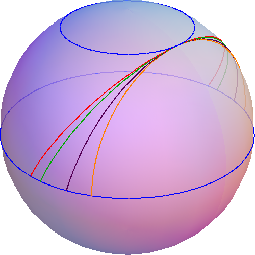
Some basic limiting cases are worth discussing at this point. The HM [4] solution (1) corresponds to taking $\omega=1$ and $J=\infty$. One may obtain the closed folded GKP string (1) [5] by superimposing two of our GMs with velocity $v=0$, maximum momentum $p=\pi$ and angular momentum $J/2$. Imposing proper boundary conditions, the two Virasoro constraints for the giant magnon (A)–(A), admit the following solutions:
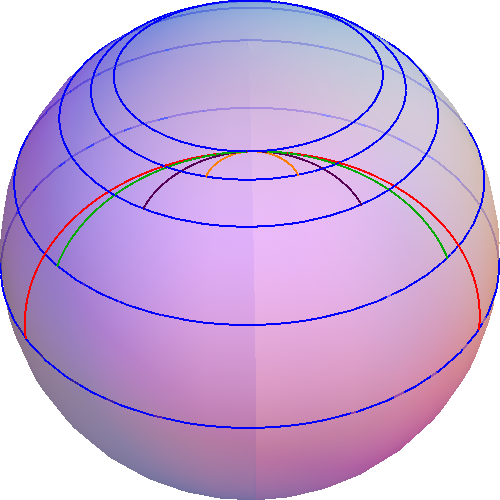
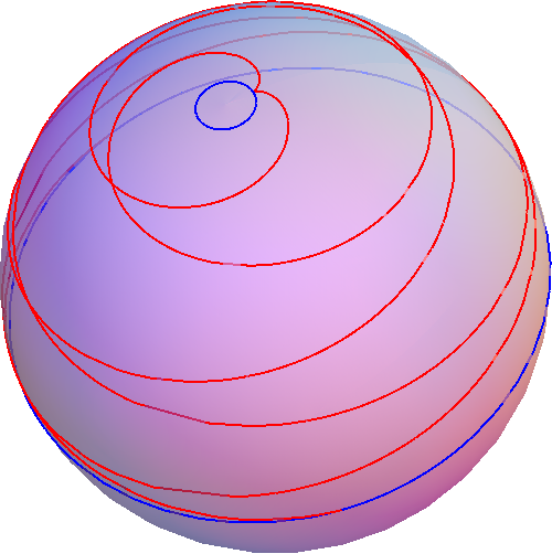
Refer to caption
Refer to caption
Figure 1: Various $\omega>1$ GMs (elementary region) for $v=\text{const.}$ (left) and $\omega=\text{const.}$ (right).
z(τσ)= R1 - v2dn(σ- vωτω η 1 - v2,η),  n ⋅r ≤σ- vωτ(n + 1)⋅r (A.23)zτσ= Rsuperscript1 - v2dnσ- vωτω η superscript1 - v2,η,  n ⋅r ≤σ- vωτn + 1⋅r (A.23)\halign to=0.0pt{\relax\global\advance\@IEEEeqncolcnt by 1\relax\begingroup\csname @IEEEeqnarraycolPREc\endcsname#\relax\relax\relax\relax\relax\relax\relax\relax\relax\relax\csname @IEEEeqnarraycolPOSTc\endcsname\relax\relax\relax\relax\relax\relax\relax\relax\relax\relax\endgroup&\global\advance\@IEEEeqncolcnt by 1\relax\bgroup#\egroup&\global\advance\@IEEEeqncolcnt by 1\relax\hbox to\z@\bgroup\hss#\egroup\cr\hfil$\displaystyle z\left(\tau, \sigma\right) = R\sqrt{1 - v^{2}} \cdot\text{dn}\left(\frac{\sigma- v\omega\tau}{\omega\,\eta\,\sqrt{1 - v^{2}}},\eta\right) \,, \quad n \cdot r \leq\sigma- v\omega\tau\leq\left(n + 1\right) \cdot r $\hfil&{\vrule width=0.0pt,height=0.0pt,depth=0.0pt}&0.0pt{\hss{\normalcolor(A.23)}}\cr}
φ(z)(-1)n1 - v2{1ωΠ([1 - 1v2]η,arcsin[1η1 - z2zmax2] η) - (A.24)- v ω F(arcsin[1η1 - z2zmax2],η)} + n + 12⋅p  ,  zmin≤z ≤zmax(A.25)φzsuperscript-1nsuperscript1 - v2{1ωΠ(delimited-[]1 - 1superscriptv2η,arcsindelimited-[]1η1 - superscriptz2superscriptsubscriptzmax2 η) - (A.24)missing-subexpression- v ω Farcsindelimited-[]1η1 - superscriptz2superscriptsubscriptzmax2,η} + n + 12subscript⋅p  ,  zminsubscript≤z ≤zmax(A.25)\halign to=0.0pt{\relax\global\advance\@IEEEeqncolcnt by 1\relax\begingroup\csname @IEEEeqnarraycolPREl\endcsname#\relax\relax\relax\relax\relax\relax\relax\relax\relax\relax\csname @IEEEeqnarraycolPOSTl\endcsname\relax\relax\relax\relax\relax\relax\relax\relax\relax\relax\endgroup&\relax\global\advance\@IEEEeqncolcnt by 1\relax\begingroup\csname @IEEEeqnarraycolPREl\endcsname#\relax\relax\relax\relax\relax\relax\relax\relax\relax\relax\csname @IEEEeqnarraycolPOSTl\endcsname\relax\relax\relax\relax\relax\relax\relax\relax\relax\relax\endgroup&\global\advance\@IEEEeqncolcnt by 1\relax\bgroup#\egroup&\global\advance\@IEEEeqncolcnt by 1\relax\hbox to\z@\bgroup\hss#\egroup\cr$\displaystyle\varphi\left(z\right) = \frac{\left(-1\right)^{n}}{\sqrt{1 - v^{2}}} $\hfil&$\displaystyle\Bigg{\{}\frac{1}{v \omega} \, \boldsymbol{\Pi}\Bigg{(}\left[1 - \frac{1}{v^{2}}\right]\eta,\arcsin\left[\frac{1}{\sqrt{\eta}}\sqrt{1 - \frac{z^{2}}{z_{\text{max}}^{2}}}\right]\bigg{|}\,\eta\Bigg{)} - $\hfil&{{}\vrule width=0.0pt,height=0.0pt,depth=0.0pt}&0.0pt{\hss{\normalcolor(A.24)}}\cr\penalty 0\vskip 3.0pt\vskip 12.0pt\cr$\displaystyle$\hfil&$\displaystyle- v \omega\,\mathbb{F}\left(\arcsin\left[\frac{1}{\sqrt{\eta}}\sqrt{1 - \frac{z^{2}}{z_{\text{max}}^{2}}}\right],\eta\right)\Bigg{\}} + \left\lfloor\frac{n + 1}{2}\right\rfloor\cdot p \,, \quad z_{\text{min}} \leq z \leq z_{\text{max}}, \qquad $\hfil&{\vrule width=0.0pt,height=0.0pt,depth=0.0pt}&0.0pt{\hss{\normalcolor(A.25)}}\cr}

where $\lfloor y\rfloor$ is the floor function of $y$. One may draw instantanés of giant magnons, by plotting (A.1) on a sphere for various values of the velocities $v$ and $\omega$, $-r\leq\sigma\leq r$ and $\tau=0$. See figure 1. Using $\mathsf{Mathematica}$ one may also animate these magnons, obtaining the worm-like motion that has been described in [17]. According to the Okamura-Suzuki terminology [54], this is a single-spin helical string of type (i).
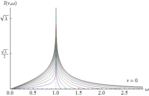
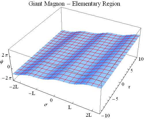
The periodic sine-Gordon solitons that are obtained from the corresponding Pohlmeyer reduction can be found from equation (A):

ψ(τσ)π2am(σ- vωτω η 1 - v2,η)(A.26)ψτσπ2amσ- vωτω η superscript1 - v2,ηmissing-subexpression(A.26)\halign to=0.0pt{\relax\global\advance\@IEEEeqncolcnt by 1\relax\begingroup\csname @IEEEeqnarraycolPREl\endcsname#\relax\relax\relax\relax\relax\relax\relax\relax\relax\relax\csname @IEEEeqnarraycolPOSTl\endcsname\relax\relax\relax\relax\relax\relax\relax\relax\relax\relax\endgroup&\relax\global\advance\@IEEEeqncolcnt by 1\relax\begingroup\csname @IEEEeqnarraycolPREl\endcsname#\relax\relax\relax\relax\relax\relax\relax\relax\relax\relax\csname @IEEEeqnarraycolPOSTl\endcsname\relax\relax\relax\relax\relax\relax\relax\relax\relax\relax\endgroup&\global\advance\@IEEEeqncolcnt by 1\relax\bgroup#\egroup&\global\advance\@IEEEeqncolcnt by 1\relax\hbox to\z@\bgroup\hss#\egroup\cr$\displaystyle\psi\left(\tau, \sigma\right) = \frac{\pi}{2} + \text{am}\left(\frac{\sigma- v\omega\tau}{\omega\,\eta\,\sqrt{1 - v^{2}}},\eta\right). \qquad $\hfil&$\displaystyle$\hfil&{\vrule width=0.0pt,height=0.0pt,depth=0.0pt}&0.0pt{\hss{\normalcolor(A.26)}}\cr}

As described in [19] this solution describes a quasi-periodic series of sG kinks, also known as kink chain/train. The period of the kink train is given by

ψ(τσ)ψ(σ+ L,τ)+ nπ ,  L = 2η(1 - v2ω2)K(η),  n = 0,±1,±2, …(A.27)ψτσψσ+ L,τ+ nπ ,  L = 2ηsuperscript1 - v2superscriptω2Kη,  n = 0,±1,±2, …missing-subexpression(A.27)\halign to=0.0pt{\relax\global\advance\@IEEEeqncolcnt by 1\relax\begingroup\csname @IEEEeqnarraycolPREl\endcsname#\relax\relax\relax\relax\relax\relax\relax\relax\relax\relax\csname @IEEEeqnarraycolPOSTl\endcsname\relax\relax\relax\relax\relax\relax\relax\relax\relax\relax\endgroup&\relax\global\advance\@IEEEeqncolcnt by 1\relax\begingroup\csname @IEEEeqnarraycolPREl\endcsname#\relax\relax\relax\relax\relax\relax\relax\relax\relax\relax\csname @IEEEeqnarraycolPOSTl\endcsname\relax\relax\relax\relax\relax\relax\relax\relax\relax\relax\endgroup&\global\advance\@IEEEeqncolcnt by 1\relax\bgroup#\egroup&\global\advance\@IEEEeqncolcnt by 1\relax\hbox to\z@\bgroup\hss#\egroup\cr$\displaystyle\psi\left(\tau, \sigma\right) = \psi\left(\sigma+ L,\tau\right) + n\pi\,, \quad L = 2\sqrt{\eta\left(1 - v^{2}\omega^{2}\right)} \cdot\mathbb{K}\left(\eta\right)\,, \quad n = 0,\pm 1,\pm 2, \ldots$\hfil&$\displaystyle$\hfil&{\vrule width=0.0pt,height=0.0pt,depth=0.0pt}&0.0pt{\hss{\normalcolor(A.27)}}\cr}

The above solution has been plotted in figure 6 for $v=0.1$ and $\omega=1.01$. It corresponds to a linearly stable subluminal ($v\cdot\omega<1$) rotational wave, according to [55].

A.2 Giant Magnon: Doubled Region,  $0\leq\left|v\right|\leq 1\leq 1/\omega$

This is the case where

ζω2= - zmin2≤0 ≤z2≤zmax2ζv2≤R2(A.28)subscriptsuperscriptζ2ωsuperscriptsubscript= - zmin2superscript≤0 ≤z2superscriptsubscript≤zmax2subscriptsuperscriptζ2vsuperscript≤R2(A.28)\halign to=0.0pt{\relax\global\advance\@IEEEeqncolcnt by 1\relax\begingroup\csname @IEEEeqnarraycolPREc\endcsname#\relax\relax\relax\relax\relax\relax\relax\relax\relax\relax\csname @IEEEeqnarraycolPOSTc\endcsname\relax\relax\relax\relax\relax\relax\relax\relax\relax\relax\endgroup&\global\advance\@IEEEeqncolcnt by 1\relax\bgroup#\egroup&\global\advance\@IEEEeqncolcnt by 1\relax\hbox to\z@\bgroup\hss#\egroup\cr\hfil$\displaystyle\zeta^{2}_{\omega} = - z_{\text{min}}^{2} \leq 0 \leq z^{2} \leq z_{\text{max}}^{2} = \zeta^{2}_{v} \leq R^{2}. $\hfil&{\vrule width=0.0pt,height=0.0pt,depth=0.0pt}&0.0pt{\hss{\normalcolor(A.28)}}\cr}

The string’s conserved momentum is given by the formula

p ≡Δϕ= Δφ= ∫-r+rφ’   dσ2ω1 - v2ω2[1ωΠ(1 - 1v21η)- v ω K(1η)](A.29)superscriptsubscriptp ≡Δϕ= Δφ= ∫-r+rφ’   dσ2ωsuperscript1 - v2superscriptω2delimited-[]1ωΠ1 - 1superscriptv21η- v ω K1ηmissing-subexpression(A.29)\halign to=0.0pt{\relax\global\advance\@IEEEeqncolcnt by 1\relax\begingroup\csname @IEEEeqnarraycolPREl\endcsname#\relax\relax\relax\relax\relax\relax\relax\relax\relax\relax\csname @IEEEeqnarraycolPOSTl\endcsname\relax\relax\relax\relax\relax\relax\relax\relax\relax\relax\endgroup&\relax\global\advance\@IEEEeqncolcnt by 1\relax\begingroup\csname @IEEEeqnarraycolPREl\endcsname#\relax\relax\relax\relax\relax\relax\relax\relax\relax\relax\csname @IEEEeqnarraycolPOSTl\endcsname\relax\relax\relax\relax\relax\relax\relax\relax\relax\relax\endgroup&\global\advance\@IEEEeqncolcnt by 1\relax\bgroup#\egroup&\global\advance\@IEEEeqncolcnt by 1\relax\hbox to\z@\bgroup\hss#\egroup\cr$\displaystyle p \equiv\Delta\phi= \Delta\varphi= \int_{-r}^{+r} \varphi' \, d\sigma= \frac{2\omega}{\sqrt{1 - v^{2} \omega^{2}}}\left[\frac{1}{v \omega} \, \boldsymbol{\Pi}\left(1 - \frac{1}{v^{2}}; \frac{1}{\eta}\right) - v \omega\, \mathbb{K}\left(\frac{1}{\eta}\right)\right], $\hfil&$\displaystyle$\hfil&{\vrule width=0.0pt,height=0.0pt,depth=0.0pt}&0.0pt{\hss{\normalcolor(A.29)}}\cr}

where again we have defined,

η≡1 + zmin2zmax21 - v2ω2ω2(1 - v2)ω1η+ v2(1 - η)(A.30)η≡1 + subscriptsuperscriptz2minsubscriptsuperscriptz2maxsuperscript1 - v2superscriptω2superscriptω2superscript1 - v2ω1superscriptη+ v21 - ηmissing-subexpression(A.30)\halign to=0.0pt{\relax\global\advance\@IEEEeqncolcnt by 1\relax\begingroup\csname @IEEEeqnarraycolPREl\endcsname#\relax\relax\relax\relax\relax\relax\relax\relax\relax\relax\csname @IEEEeqnarraycolPOSTl\endcsname\relax\relax\relax\relax\relax\relax\relax\relax\relax\relax\endgroup&\relax\global\advance\@IEEEeqncolcnt by 1\relax\begingroup\csname @IEEEeqnarraycolPREl\endcsname#\relax\relax\relax\relax\relax\relax\relax\relax\relax\relax\csname @IEEEeqnarraycolPOSTl\endcsname\relax\relax\relax\relax\relax\relax\relax\relax\relax\relax\endgroup&\global\advance\@IEEEeqncolcnt by 1\relax\bgroup#\egroup&\global\advance\@IEEEeqncolcnt by 1\relax\hbox to\z@\bgroup\hss#\egroup\cr$\displaystyle\eta\equiv 1 + \frac{z^{2}_{\text{min}}}{z^{2}_{\text{max}}} = \frac{1 - v^{2} \omega^{2}}{\omega^{2}\left(1 - v^{2}\right)} \Leftrightarrow\omega= \frac{1}{\sqrt{\eta+ v^{2}\left(1 - \eta\right)}}. $\hfil&$\displaystyle$\hfil&{\vrule width=0.0pt,height=0.0pt,depth=0.0pt}&0.0pt{\hss{\normalcolor(A.30)}}\cr}

Refer to caption
Refer to caption
Refer to caption
Figure 2: Momentum, energy and spin of the giant magnon as functions of its angular velocity $\omega$.

The open string’s conserved energy and angular momentum are given by:

E = λ2π-r+rt˙dσλπλπ1 - v2ω2K(1η),  r = 1 - v2ω2K(1η)(A.31)J = λ2πR2-r+r(R2- z2)ϕ˙dσλπ1 - v2ω2ω[K(1η)E(1η)](A.32)E = λ2πsuperscriptsubscript-r+r˙tdσλπλπsuperscript1 - v2superscriptω2K1η,  r = superscript1 - v2superscriptω2K1ηmissing-subexpression(A.31)missing-subexpressionJ = λsuperscript2πR2superscriptsubscript-r+rsuperscriptR2superscript- z2˙ϕdσλπsuperscript1 - v2superscriptω2ωdelimited-[]K1ηE1ηmissing-subexpression(A.32)\halign to=0.0pt{\relax\global\advance\@IEEEeqncolcnt by 1\relax\begingroup\csname @IEEEeqnarraycolPREl\endcsname#\relax\relax\relax\relax\relax\relax\relax\relax\relax\relax\csname @IEEEeqnarraycolPOSTl\endcsname\relax\relax\relax\relax\relax\relax\relax\relax\relax\relax\endgroup&\relax\global\advance\@IEEEeqncolcnt by 1\relax\begingroup\csname @IEEEeqnarraycolPREl\endcsname#\relax\relax\relax\relax\relax\relax\relax\relax\relax\relax\csname @IEEEeqnarraycolPOSTl\endcsname\relax\relax\relax\relax\relax\relax\relax\relax\relax\relax\endgroup&\global\advance\@IEEEeqncolcnt by 1\relax\bgroup#\egroup&\global\advance\@IEEEeqncolcnt by 1\relax\hbox to\z@\bgroup\hss#\egroup\cr$\displaystyle E = \frac{\sqrt{\lambda}}{2\pi} \int_{-r}^{+r} \dot{t} \, d\sigma= \frac{r\,\sqrt{\lambda}}{\pi} = \frac{\sqrt{\lambda}}{\pi}\cdot\sqrt{1 - v^{2}\omega^{2}}\,\mathbb{K}\left(\frac{1}{\eta}\right)\,, \quad r = \sqrt{1 - v^{2}\omega^{2}}\,\mathbb{K}\left(\frac{1}{\eta}\right) $\hfil&$\displaystyle{}$\hfil&{\vrule width=0.0pt,height=0.0pt,depth=0.0pt}&0.0pt{\hss{\normalcolor(A.31)}}\cr\penalty 0\vskip 3.0pt\vskip 12.0pt\cr$\displaystyle J = \frac{\sqrt{\lambda}}{2\pi R^{2}} \int_{-r}^{+r} \left(R^{2} - z^{2}\right)\dot{\phi} \, d\sigma= \frac{\sqrt{\lambda}}{\pi}\cdot\frac{\sqrt{1 - v^{2} \omega^{2}}}{\omega} \, \left[\mathbb{K}\left(\frac{1}{\eta}\right) - \mathbb{E}\left(\frac{1}{\eta}\right)\right]. $\hfil&$\displaystyle$\hfil&{\vrule width=0.0pt,height=0.0pt,depth=0.0pt}&0.0pt{\hss{\normalcolor(A.32)}}\cr}

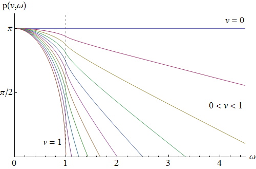
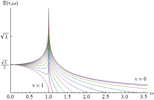
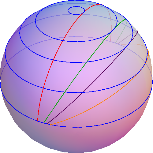
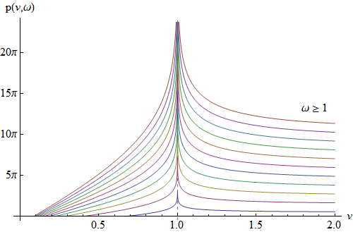
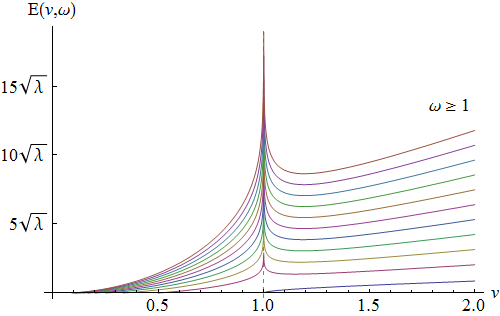
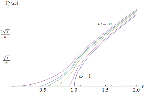
In figure 2 we have plotted the momentum, energy and spin of the giant magnon in terms of its angular velocity $\omega$ for various values of the velocity $v$, in both the elementary ($\omega\geq 1$) and the doubled ($\omega\leq 1$) region. The Virasoro constraints (A)–(A) with the appropriate boundary conditions are solved by:

z(τσ)= R1 - v2cn(σ- vωτ1 - v2ω2,1η),  2   n ⋅r ≤σ- vωτ≤2(n + 1)⋅r (A.33)zτσ= Rsuperscript1 - v2cnσ- vωτsuperscript1 - v2superscriptω2,1η,  2   n ⋅r ≤σ- vωτ≤2n + 1⋅r (A.33)\halign to=0.0pt{\relax\global\advance\@IEEEeqncolcnt by 1\relax\begingroup\csname @IEEEeqnarraycolPREc\endcsname#\relax\relax\relax\relax\relax\relax\relax\relax\relax\relax\csname @IEEEeqnarraycolPOSTc\endcsname\relax\relax\relax\relax\relax\relax\relax\relax\relax\relax\endgroup&\global\advance\@IEEEeqncolcnt by 1\relax\bgroup#\egroup&\global\advance\@IEEEeqncolcnt by 1\relax\hbox to\z@\bgroup\hss#\egroup\cr\hfil$\displaystyle z\left(\tau, \sigma\right) = R\sqrt{1 - v^{2}} \cdot\text{cn}\left(\frac{\sigma- v\omega\tau}{\sqrt{1 - v^{2} \omega^{2}}},\frac{1}{\eta}\right)\,, \quad 2 \, n \cdot r \leq\sigma- v\omega\tau\leq 2\left(n + 1\right) \cdot r $\hfil&{\vrule width=0.0pt,height=0.0pt,depth=0.0pt}&0.0pt{\hss{\normalcolor(A.33)}}\cr}
φ(z)(-1)nω1 - v2ω2{1ωΠ(1 - 1v2,arccos[zzmax] 1η) - (A.34)- v ω F(arccos[zzmax],1η)} + 2n + 12⋅p ,  -zmax≤z ≤zmax(A.35)φzsuperscript-1nωsuperscript1 - v2superscriptω2{1ωΠ(1 - 1superscriptv2,arccosdelimited-[]zsubscriptzmax 1η) - (A.34)missing-subexpression- v ω Farccosdelimited-[]zsubscriptzmax,1η} + 2n + 12subscript⋅p ,  -zmaxsubscript≤z ≤zmax(A.35)\halign to=0.0pt{\relax\global\advance\@IEEEeqncolcnt by 1\relax\begingroup\csname @IEEEeqnarraycolPREl\endcsname#\relax\relax\relax\relax\relax\relax\relax\relax\relax\relax\csname @IEEEeqnarraycolPOSTl\endcsname\relax\relax\relax\relax\relax\relax\relax\relax\relax\relax\endgroup&\relax\global\advance\@IEEEeqncolcnt by 1\relax\begingroup\csname @IEEEeqnarraycolPREl\endcsname#\relax\relax\relax\relax\relax\relax\relax\relax\relax\relax\csname @IEEEeqnarraycolPOSTl\endcsname\relax\relax\relax\relax\relax\relax\relax\relax\relax\relax\endgroup&\global\advance\@IEEEeqncolcnt by 1\relax\bgroup#\egroup&\global\advance\@IEEEeqncolcnt by 1\relax\hbox to\z@\bgroup\hss#\egroup\cr$\displaystyle\varphi\left(z\right) = \frac{\left(-1\right)^{n}\,\omega}{\sqrt{1 - v^{2} \omega^{2}}} \Bigg{\{}\frac{1}{v \omega} \,$\hfil&$\displaystyle\boldsymbol{\Pi}\Bigg{(}1 - \frac{1}{v^{2}},\arccos\left[\frac{z}{z_{\text{max}}}\right]\bigg{|}\,\frac{1}{\eta}\Bigg{)} - $\hfil&{{}\vrule width=0.0pt,height=0.0pt,depth=0.0pt}&0.0pt{\hss{\normalcolor(A.34)}}\cr\penalty 0\vskip 3.0pt\vskip 12.0pt\cr$\displaystyle$\hfil&$\displaystyle- v \omega\, \mathbb{F}\left(\arccos\left[\frac{z}{z_{\text{max}}}\right],\frac{1}{\eta}\right)\Bigg{\}} + 2\left\lfloor\frac{n + 1}{2}\right\rfloor\cdot p\,, \quad-z_{\text{max}} \leq z \leq z_{\text{max}}. \qquad $\hfil&{\vrule width=0.0pt,height=0.0pt,depth=0.0pt}&0.0pt{\hss{\normalcolor(A.35)}}\cr}

The strings in this case have been plotted for various $v$’s and $\omega$’s in figure 3. Their motion is a combination of rotation and translation, initially tangent to the parallel $z=z_{\text{max}}$, shifting gradually towards the parallel $z=-z_{\text{max}}$ of the southern hemisphere and all over again. These configurations have also been described by Okamura and Suzuki [54] as type (ii) single-spin helical strings.
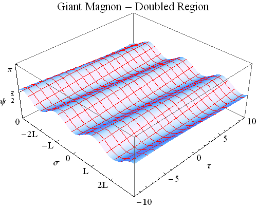
The Pohlmeyer reduction (A) gives a periodic series of sG kinks and anti-kinks (known as kink-antikink chain/train):

ψ(τσ)= arccos[1ηsn(σ- vωτ1 - v2ω2,1η)](A.36)ψτσ= arccosdelimited-[]1ηsnσ- vωτsuperscript1 - v2superscriptω2,1ηmissing-subexpression(A.36)\halign to=0.0pt{\relax\global\advance\@IEEEeqncolcnt by 1\relax\begingroup\csname @IEEEeqnarraycolPREl\endcsname#\relax\relax\relax\relax\relax\relax\relax\relax\relax\relax\csname @IEEEeqnarraycolPOSTl\endcsname\relax\relax\relax\relax\relax\relax\relax\relax\relax\relax\endgroup&\relax\global\advance\@IEEEeqncolcnt by 1\relax\begingroup\csname @IEEEeqnarraycolPREl\endcsname#\relax\relax\relax\relax\relax\relax\relax\relax\relax\relax\csname @IEEEeqnarraycolPOSTl\endcsname\relax\relax\relax\relax\relax\relax\relax\relax\relax\relax\endgroup&\global\advance\@IEEEeqncolcnt by 1\relax\bgroup#\egroup&\global\advance\@IEEEeqncolcnt by 1\relax\hbox to\z@\bgroup\hss#\egroup\cr$\displaystyle\psi\left(\tau, \sigma\right) = \arccos\left[\frac{1}{\sqrt{\eta}}\,\text{sn}\left(\frac{\sigma- v\omega\tau}{\sqrt{1 - v^{2}\omega^{2}}},\frac{1}{\eta}\right)\right], \qquad $\hfil&$\displaystyle$\hfil&{\vrule width=0.0pt,height=0.0pt,depth=0.0pt}&0.0pt{\hss{\normalcolor(A.36)}}\cr}

which we have plotted in figure 6 for $v=0.4$ and $\omega=0.3$. The half-period of the train is

ψ(τσ)= -ψ(σ+ L,τ)+ nπ ,  L = 21 - v2ω2K(1η),  n = 0,±1,±2, …(A.37)ψτσ= -ψσ+ L,τ+ nπ ,  L = 2superscript1 - v2superscriptω2K1η,  n = 0,±1,±2, …missing-subexpression(A.37)\halign to=0.0pt{\relax\global\advance\@IEEEeqncolcnt by 1\relax\begingroup\csname @IEEEeqnarraycolPREl\endcsname#\relax\relax\relax\relax\relax\relax\relax\relax\relax\relax\csname @IEEEeqnarraycolPOSTl\endcsname\relax\relax\relax\relax\relax\relax\relax\relax\relax\relax\endgroup&\relax\global\advance\@IEEEeqncolcnt by 1\relax\begingroup\csname @IEEEeqnarraycolPREl\endcsname#\relax\relax\relax\relax\relax\relax\relax\relax\relax\relax\csname @IEEEeqnarraycolPOSTl\endcsname\relax\relax\relax\relax\relax\relax\relax\relax\relax\relax\endgroup&\global\advance\@IEEEeqncolcnt by 1\relax\bgroup#\egroup&\global\advance\@IEEEeqncolcnt by 1\relax\hbox to\z@\bgroup\hss#\egroup\cr$\displaystyle\psi\left(\tau, \sigma\right) = -\psi\left(\sigma+ L,\tau\right) + n\pi\,, \quad L = 2\sqrt{1 - v^{2}\omega^{2}} \cdot\mathbb{K}\left(\frac{1}{\eta}\right)\,, \quad n = 0,\pm 1,\pm 2, \ldots$\hfil&$\displaystyle$\hfil&{\vrule width=0.0pt,height=0.0pt,depth=0.0pt}&0.0pt{\hss{\normalcolor(A.37)}}\cr}

It’s a spectrally unstable subluminal ($v\cdot\omega<1$) librational wave [55].

Refer to caption
Refer to caption
Figure 3: $\omega<1$ giant magnons (doubled region) with $v=\text{const.}$ (left) or $\omega=\text{const.}$ (right).

A.3 Single Spike: Elementary Region,  $0\leq 1/\omega<\left|v\right|\leq 1$

In this case,

0 ≤ζv2= zmin2≤z2≤zmax2ζω2≤R2(A.38)subscriptsuperscript0 ≤ζ2vsuperscriptsubscript= zmin2superscript≤z2superscriptsubscript≤zmax2subscriptsuperscriptζ2ωsuperscript≤R2(A.38)\halign to=0.0pt{\relax\global\advance\@IEEEeqncolcnt by 1\relax\begingroup\csname @IEEEeqnarraycolPREc\endcsname#\relax\relax\relax\relax\relax\relax\relax\relax\relax\relax\csname @IEEEeqnarraycolPOSTc\endcsname\relax\relax\relax\relax\relax\relax\relax\relax\relax\relax\endgroup&\global\advance\@IEEEeqncolcnt by 1\relax\bgroup#\egroup&\global\advance\@IEEEeqncolcnt by 1\relax\hbox to\z@\bgroup\hss#\egroup\cr\hfil$\displaystyle 0 \leq\zeta^{2}_{v} = z_{\text{min}}^{2} \leq z^{2} \leq z_{\text{max}}^{2} = \zeta^{2}_{\omega} \leq R^{2}, $\hfil&{\vrule width=0.0pt,height=0.0pt,depth=0.0pt}&0.0pt{\hss{\normalcolor(A.38)}}\cr}

while the conserved momentum is found to be:

p ≡Δϕ= Δφ= ∫-r+rφ’   dσ2 v ω1 - 1/ω2[K(η)Π(1 - v2ω2η)](A.39)superscriptsubscriptp ≡Δϕ= Δφ= ∫-r+rφ’   dσ2 v ωsuperscript1 - 1/ω2[KηΠsuperscript1 - v2superscriptω2η]missing-subexpression(A.39)\halign to=0.0pt{\relax\global\advance\@IEEEeqncolcnt by 1\relax\begingroup\csname @IEEEeqnarraycolPREl\endcsname#\relax\relax\relax\relax\relax\relax\relax\relax\relax\relax\csname @IEEEeqnarraycolPOSTl\endcsname\relax\relax\relax\relax\relax\relax\relax\relax\relax\relax\endgroup&\relax\global\advance\@IEEEeqncolcnt by 1\relax\begingroup\csname @IEEEeqnarraycolPREl\endcsname#\relax\relax\relax\relax\relax\relax\relax\relax\relax\relax\csname @IEEEeqnarraycolPOSTl\endcsname\relax\relax\relax\relax\relax\relax\relax\relax\relax\relax\endgroup&\global\advance\@IEEEeqncolcnt by 1\relax\bgroup#\egroup&\global\advance\@IEEEeqncolcnt by 1\relax\hbox to\z@\bgroup\hss#\egroup\cr$\displaystyle p \equiv\Delta\phi= \Delta\varphi= \int_{-r}^{+r} \varphi' \, d\sigma= \frac{2 v \omega}{\sqrt{1 - 1/\omega^{2}}} \, \Big{[}\mathbb{K}\left(\eta\right) - \boldsymbol{\Pi}\left(1 - v^{2}\omega^{2} ; \eta\right)\Big{]}, $\hfil&$\displaystyle$\hfil&{\vrule width=0.0pt,height=0.0pt,depth=0.0pt}&0.0pt{\hss{\normalcolor(A.39)}}\cr}

with the assignment

η≡1 - zmin2zmax2v2ω2- 1ω2- 1ω1 - ηv2η(A.40)η≡1 - subscriptsuperscriptz2minsubscriptsuperscriptz2maxsuperscriptv2superscriptω2- 1superscriptω2- 1ω1 - ηsuperscriptv2ηmissing-subexpression(A.40)\halign to=0.0pt{\relax\global\advance\@IEEEeqncolcnt by 1\relax\begingroup\csname @IEEEeqnarraycolPREl\endcsname#\relax\relax\relax\relax\relax\relax\relax\relax\relax\relax\csname @IEEEeqnarraycolPOSTl\endcsname\relax\relax\relax\relax\relax\relax\relax\relax\relax\relax\endgroup&\relax\global\advance\@IEEEeqncolcnt by 1\relax\begingroup\csname @IEEEeqnarraycolPREl\endcsname#\relax\relax\relax\relax\relax\relax\relax\relax\relax\relax\csname @IEEEeqnarraycolPOSTl\endcsname\relax\relax\relax\relax\relax\relax\relax\relax\relax\relax\endgroup&\global\advance\@IEEEeqncolcnt by 1\relax\bgroup#\egroup&\global\advance\@IEEEeqncolcnt by 1\relax\hbox to\z@\bgroup\hss#\egroup\cr$\displaystyle\eta\equiv 1 - \frac{z^{2}_{\text{min}}}{z^{2}_{\text{max}}} = \frac{v^{2} \omega^{2} - 1}{\omega^{2} - 1} \Leftrightarrow\omega= \sqrt{\frac{1 - \eta}{v^{2} - \eta}}. $\hfil&$\displaystyle$\hfil&{\vrule width=0.0pt,height=0.0pt,depth=0.0pt}&0.0pt{\hss{\normalcolor(A.40)}}\cr}
Refer to caption
Refer to caption
Figure 4: Single-spike string ($v\cdot\omega>1$) in the elementary (left) and doubled region (right).

The energy and the angular momentum of the strings are given by:

E = λ2π-r+rt˙dσλπλπv2ω2- 1ω2- 1K(η),  r = v2ω2- 1ω2- 1K(η)(A.41)J = λ2πR2-r+r(R2- z2)ϕ˙dσλπ1 - 1ω2[E(η)1-v21-1/ω2K(η)](A.42)E = λ2πsuperscriptsubscript-r+r˙tdσλπλπsuperscriptv2superscriptω2- 1superscriptω2- 1Kη,  r = superscriptv2superscriptω2- 1superscriptω2- 1Kηmissing-subexpression(A.41)missing-subexpressionJ = λsuperscript2πR2superscriptsubscript-r+rsuperscriptR2superscript- z2˙ϕdσλπ1 - 1superscriptω2[Eηsuperscript1-v2superscript1-1/ω2Kη]missing-subexpression(A.42)\halign to=0.0pt{\relax\global\advance\@IEEEeqncolcnt by 1\relax\begingroup\csname @IEEEeqnarraycolPREl\endcsname#\relax\relax\relax\relax\relax\relax\relax\relax\relax\relax\csname @IEEEeqnarraycolPOSTl\endcsname\relax\relax\relax\relax\relax\relax\relax\relax\relax\relax\endgroup&\relax\global\advance\@IEEEeqncolcnt by 1\relax\begingroup\csname @IEEEeqnarraycolPREl\endcsname#\relax\relax\relax\relax\relax\relax\relax\relax\relax\relax\csname @IEEEeqnarraycolPOSTl\endcsname\relax\relax\relax\relax\relax\relax\relax\relax\relax\relax\endgroup&\global\advance\@IEEEeqncolcnt by 1\relax\bgroup#\egroup&\global\advance\@IEEEeqncolcnt by 1\relax\hbox to\z@\bgroup\hss#\egroup\cr$\displaystyle E = \frac{\sqrt{\lambda}}{2\pi} \int_{-r}^{+r} \dot{t} \, d\sigma= \frac{r\,\sqrt{\lambda}}{\pi} = \frac{\sqrt{\lambda}}{\pi}\cdot\frac{v^{2} \omega^{2} - 1}{\sqrt{\omega^{2} - 1}}\,\mathbb{K}\left(\eta\right)\,, \quad r = \frac{v^{2} \omega^{2} - 1}{\sqrt{\omega^{2} - 1}}\,\mathbb{K}\left(\eta\right) $\hfil&$\displaystyle{}$\hfil&{\vrule width=0.0pt,height=0.0pt,depth=0.0pt}&0.0pt{\hss{\normalcolor(A.41)}}\cr\penalty 0\vskip 3.0pt\vskip 12.0pt\cr$\displaystyle J = \frac{\sqrt{\lambda}}{2\pi R^{2}} \int_{-r}^{+r} \left(R^{2} - z^{2}\right)\dot{\phi} \, d\sigma= \frac{\sqrt{\lambda}}{\pi} \cdot\sqrt{1 - \frac{1}{\omega^{2}}} \, \bigg{[}\mathbb{E}\left(\eta\right) - \frac{1-v^{2}}{1-1/\omega^{2}}\,\mathbb{K}\left(\eta\right)\bigg{]}. $\hfil&$\displaystyle$\hfil&{\vrule width=0.0pt,height=0.0pt,depth=0.0pt}&0.0pt{\hss{\normalcolor(A.42)}}\cr}

Equations (A)–(A) have the following solutions:

z(τσ)= R1 - 1ω2dn(σ- vωτηω2- 1,η)(A.43)zτσ= R1 - 1superscriptω2dnσ- vωτηsuperscriptω2- 1,η(A.43)\halign to=0.0pt{\relax\global\advance\@IEEEeqncolcnt by 1\relax\begingroup\csname @IEEEeqnarraycolPREc\endcsname#\relax\relax\relax\relax\relax\relax\relax\relax\relax\relax\csname @IEEEeqnarraycolPOSTc\endcsname\relax\relax\relax\relax\relax\relax\relax\relax\relax\relax\endgroup&\global\advance\@IEEEeqncolcnt by 1\relax\bgroup#\egroup&\global\advance\@IEEEeqncolcnt by 1\relax\hbox to\z@\bgroup\hss#\egroup\cr\hfil$\displaystyle z\left(\tau, \sigma\right) = R\sqrt{1 - \frac{1}{\omega^{2}}} \cdot\text{dn}\left(\frac{\sigma- v\omega\tau}{\eta\sqrt{\omega^{2} - 1}},\eta\right) $\hfil&{\vrule width=0.0pt,height=0.0pt,depth=0.0pt}&0.0pt{\hss{\normalcolor(A.43)}}\cr}
φ(z)(-1)nω1 - 1/ω2{F(arcsin[1η1 - z2zmax2],η) - (A.44) - Π(1 - v2ω2,arcsin[1η1 - z2zmax2] η)} + n + 12⋅p  ,  zmin≤z ≤zmax(A.45)φzsuperscript-1nωsuperscript1 - 1/ω2{F(arcsindelimited-[]1η1 - superscriptz2superscriptsubscriptzmax2,η) - (A.44)missing-subexpressionsuperscript - Π(1 - v2superscriptω2,arcsindelimited-[]1η1 - superscriptz2superscriptsubscriptzmax2 η)} + n + 12subscript⋅p  ,  zminsubscript≤z ≤zmax(A.45)\halign to=0.0pt{\relax\global\advance\@IEEEeqncolcnt by 1\relax\begingroup\csname @IEEEeqnarraycolPREl\endcsname#\relax\relax\relax\relax\relax\relax\relax\relax\relax\relax\csname @IEEEeqnarraycolPOSTl\endcsname\relax\relax\relax\relax\relax\relax\relax\relax\relax\relax\endgroup&\relax\global\advance\@IEEEeqncolcnt by 1\relax\begingroup\csname @IEEEeqnarraycolPREl\endcsname#\relax\relax\relax\relax\relax\relax\relax\relax\relax\relax\csname @IEEEeqnarraycolPOSTl\endcsname\relax\relax\relax\relax\relax\relax\relax\relax\relax\relax\endgroup&\global\advance\@IEEEeqncolcnt by 1\relax\bgroup#\egroup&\global\advance\@IEEEeqncolcnt by 1\relax\hbox to\z@\bgroup\hss#\egroup\cr$\displaystyle\varphi\left(z\right) = $\hfil&$\displaystyle\frac{\left(-1\right)^{n}\,v \omega}{\sqrt{1 - 1/\omega^{2}}} \Bigg{\{}\mathbb{F}\bigg{(}\arcsin\left[\frac{1}{\sqrt{\eta}}\sqrt{1 - \frac{z^{2}}{z_{\text{max}}^{2}}}\right],\eta\bigg{)} - $\hfil&{{}\vrule width=0.0pt,height=0.0pt,depth=0.0pt}&0.0pt{\hss{\normalcolor(A.44)}}\cr\penalty 0\vskip 3.0pt\vskip 12.0pt\cr$\displaystyle$\hfil&$\displaystyle\hskip 14.22636pt - \boldsymbol{\Pi}\Bigg{(}1 - v^{2}\omega^{2},\arcsin\left[\frac{1}{\sqrt{\eta}}\sqrt{1 - \frac{z^{2}}{z_{\text{max}}^{2}}}\right]\bigg{|}\,\eta\Bigg{)}\Bigg{\}} + \left\lfloor\frac{n + 1}{2}\right\rfloor\cdot p \,, \quad z_{\text{min}} \leq z \leq z_{\text{max}}. \qquad $\hfil&{\vrule width=0.0pt,height=0.0pt,depth=0.0pt}&0.0pt{\hss{\normalcolor(A.45)}}\cr}

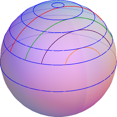
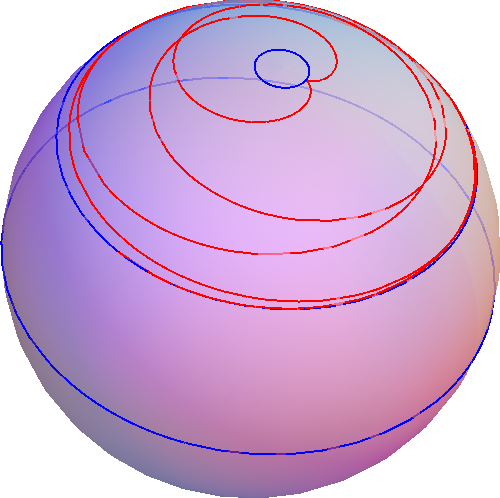
Single spike strings in the elementary region may be visualized by plotting equation (A.3) on a sphere, giving the shape pictured on the left of figure 4. Apart from the winding, their motion resembles that of elementary giant magnons in §A.1. For $v=1$, $p=\infty$ we obtain the infinite-size single spike (1) of references [35, 36].
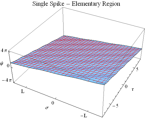
The Pohlmeyer reduction in this case reads:

ψ(τσ)am(σ- vωτη ω2- 1,η)(A.46)ψτσamσ- vωτη superscriptω2- 1,ηmissing-subexpression(A.46)\halign to=0.0pt{\relax\global\advance\@IEEEeqncolcnt by 1\relax\begingroup\csname @IEEEeqnarraycolPREl\endcsname#\relax\relax\relax\relax\relax\relax\relax\relax\relax\relax\csname @IEEEeqnarraycolPOSTl\endcsname\relax\relax\relax\relax\relax\relax\relax\relax\relax\relax\endgroup&\relax\global\advance\@IEEEeqncolcnt by 1\relax\begingroup\csname @IEEEeqnarraycolPREl\endcsname#\relax\relax\relax\relax\relax\relax\relax\relax\relax\relax\csname @IEEEeqnarraycolPOSTl\endcsname\relax\relax\relax\relax\relax\relax\relax\relax\relax\relax\endgroup&\global\advance\@IEEEeqncolcnt by 1\relax\bgroup#\egroup&\global\advance\@IEEEeqncolcnt by 1\relax\hbox to\z@\bgroup\hss#\egroup\cr$\displaystyle\psi\left(\tau, \sigma\right) = \text{am}\left(\frac{\sigma- v\omega\tau}{\eta\,\sqrt{\omega^{2} - 1}},\eta\right). \qquad $\hfil&$\displaystyle$\hfil&{\vrule width=0.0pt,height=0.0pt,depth=0.0pt}&0.0pt{\hss{\normalcolor(A.46)}}\cr}

This is again a kink chain/train, similar to that in §A.1. See its plot for $v=0.9$ and $\omega=2$ in figure 6. The period of the kink train is

ψ(τσ)ψ(σ+ L,τ)+ nπ ,  L = 2η(v2ω2- 1)K(η),  n = 0,±1,±2, …(A.47)ψτσψσ+ L,τ+ nπ ,  L = 2ηsuperscriptv2superscriptω2- 1Kη,  n = 0,±1,±2, …missing-subexpression(A.47)\halign to=0.0pt{\relax\global\advance\@IEEEeqncolcnt by 1\relax\begingroup\csname @IEEEeqnarraycolPREl\endcsname#\relax\relax\relax\relax\relax\relax\relax\relax\relax\relax\csname @IEEEeqnarraycolPOSTl\endcsname\relax\relax\relax\relax\relax\relax\relax\relax\relax\relax\endgroup&\relax\global\advance\@IEEEeqncolcnt by 1\relax\begingroup\csname @IEEEeqnarraycolPREl\endcsname#\relax\relax\relax\relax\relax\relax\relax\relax\relax\relax\csname @IEEEeqnarraycolPOSTl\endcsname\relax\relax\relax\relax\relax\relax\relax\relax\relax\relax\endgroup&\global\advance\@IEEEeqncolcnt by 1\relax\bgroup#\egroup&\global\advance\@IEEEeqncolcnt by 1\relax\hbox to\z@\bgroup\hss#\egroup\cr$\displaystyle\psi\left(\tau, \sigma\right) = \psi\left(\sigma+ L,\tau\right) + n\pi\,, \quad L = 2\sqrt{\eta\left(v^{2}\omega^{2} - 1\right)} \cdot\mathbb{K}\left(\eta\right)\,, \quad n = 0,\pm 1,\pm 2, \ldots$\hfil&$\displaystyle$\hfil&{\vrule width=0.0pt,height=0.0pt,depth=0.0pt}&0.0pt{\hss{\normalcolor(A.47)}}\cr}

and it corresponds to a spectrally unstable superluminal ($v\cdot\omega>1$) rotational wave [55].

Refer to caption
Refer to caption
Refer to caption
Figure 5: Momentum, energy and spin of the single spike as functions of its linear velocity $v$.

A.4 Single Spike: Doubled Region,  $0\leq 1/\omega\leq 1\leq\left|v\right|$

In this case the open string of S2 is bound to move between

ζv2= - zmin2≤0 ≤z2≤zmax2ζω2≤R2(A.48)subscriptsuperscriptζ2vsuperscriptsubscript= - zmin2superscript≤0 ≤z2superscriptsubscript≤zmax2subscriptsuperscriptζ2ωsuperscript≤R2(A.48)\halign to=0.0pt{\relax\global\advance\@IEEEeqncolcnt by 1\relax\begingroup\csname @IEEEeqnarraycolPREc\endcsname#\relax\relax\relax\relax\relax\relax\relax\relax\relax\relax\csname @IEEEeqnarraycolPOSTc\endcsname\relax\relax\relax\relax\relax\relax\relax\relax\relax\relax\endgroup&\global\advance\@IEEEeqncolcnt by 1\relax\bgroup#\egroup&\global\advance\@IEEEeqncolcnt by 1\relax\hbox to\z@\bgroup\hss#\egroup\cr\hfil$\displaystyle\zeta^{2}_{v} = - z_{\text{min}}^{2} \leq 0 \leq z^{2} \leq z_{\text{max}}^{2} = \zeta^{2}_{\omega} \leq R^{2}, $\hfil&{\vrule width=0.0pt,height=0.0pt,depth=0.0pt}&0.0pt{\hss{\normalcolor(A.48)}}\cr}

with momentum

p ≡Δϕ= Δφ= ∫-r+rφ’   dσ2 v ω2v2ω2- 1[K(1η)Π(1 - ω21η)](A.49)superscriptsubscriptp ≡Δϕ= Δφ= ∫-r+rφ’   dσsuperscript2 v ω2superscriptv2superscriptω2- 1delimited-[]K1ηΠsuperscript1 - ω21ηmissing-subexpression(A.49)\halign to=0.0pt{\relax\global\advance\@IEEEeqncolcnt by 1\relax\begingroup\csname @IEEEeqnarraycolPREl\endcsname#\relax\relax\relax\relax\relax\relax\relax\relax\relax\relax\csname @IEEEeqnarraycolPOSTl\endcsname\relax\relax\relax\relax\relax\relax\relax\relax\relax\relax\endgroup&\relax\global\advance\@IEEEeqncolcnt by 1\relax\begingroup\csname @IEEEeqnarraycolPREl\endcsname#\relax\relax\relax\relax\relax\relax\relax\relax\relax\relax\csname @IEEEeqnarraycolPOSTl\endcsname\relax\relax\relax\relax\relax\relax\relax\relax\relax\relax\endgroup&\global\advance\@IEEEeqncolcnt by 1\relax\bgroup#\egroup&\global\advance\@IEEEeqncolcnt by 1\relax\hbox to\z@\bgroup\hss#\egroup\cr$\displaystyle p \equiv\Delta\phi= \Delta\varphi= \int_{-r}^{+r} \varphi' \, d\sigma= \frac{2 v \omega^{2}}{\sqrt{v^{2} \omega^{2} - 1}}\left[\mathbb{K}\left(\frac{1}{\eta}\right) - \boldsymbol{\Pi}\left(1 - \omega^{2}; \frac{1}{\eta}\right)\right]. $\hfil&$\displaystyle$\hfil&{\vrule width=0.0pt,height=0.0pt,depth=0.0pt}&0.0pt{\hss{\normalcolor(A.49)}}\cr}

Again, we have defined,

η≡1 + zmin2zmax2v2ω2- 1ω2- 1ω1 - ηv2η(A.50)η≡1 + subscriptsuperscriptz2minsubscriptsuperscriptz2maxsuperscriptv2superscriptω2- 1superscriptω2- 1ω1 - ηsuperscriptv2ηmissing-subexpression(A.50)\halign to=0.0pt{\relax\global\advance\@IEEEeqncolcnt by 1\relax\begingroup\csname @IEEEeqnarraycolPREl\endcsname#\relax\relax\relax\relax\relax\relax\relax\relax\relax\relax\csname @IEEEeqnarraycolPOSTl\endcsname\relax\relax\relax\relax\relax\relax\relax\relax\relax\relax\endgroup&\relax\global\advance\@IEEEeqncolcnt by 1\relax\begingroup\csname @IEEEeqnarraycolPREl\endcsname#\relax\relax\relax\relax\relax\relax\relax\relax\relax\relax\csname @IEEEeqnarraycolPOSTl\endcsname\relax\relax\relax\relax\relax\relax\relax\relax\relax\relax\endgroup&\global\advance\@IEEEeqncolcnt by 1\relax\bgroup#\egroup&\global\advance\@IEEEeqncolcnt by 1\relax\hbox to\z@\bgroup\hss#\egroup\cr$\displaystyle\eta\equiv 1 + \frac{z^{2}_{\text{min}}}{z^{2}_{\text{max}}} = \frac{v^{2} \omega^{2} - 1}{\omega^{2} - 1} \Leftrightarrow\omega= \sqrt{\frac{1 - \eta}{v^{2} - \eta}}. $\hfil&$\displaystyle$\hfil&{\vrule width=0.0pt,height=0.0pt,depth=0.0pt}&0.0pt{\hss{\normalcolor(A.50)}}\cr}

The conserved energy and angular momentum of the open string are given by:

E = λ2π-r+rt˙dσλπλπv2ω2- 1K(1η),  r = v2ω2- 1K(1η)(A.51)J = λ2πR2-r+r(R2- z2)ϕ˙dσλπv2ω2- 1ωE(1η)(A.52)E = λ2πsuperscriptsubscript-r+r˙tdσλπλπsuperscriptv2superscriptω2- 1K1η,  r = superscriptv2superscriptω2- 1K1ηmissing-subexpression(A.51)missing-subexpressionJ = λsuperscript2πR2superscriptsubscript-r+rsuperscriptR2superscript- z2˙ϕdσλπsuperscriptv2superscriptω2- 1ωE1ηmissing-subexpression(A.52)\halign to=0.0pt{\relax\global\advance\@IEEEeqncolcnt by 1\relax\begingroup\csname @IEEEeqnarraycolPREl\endcsname#\relax\relax\relax\relax\relax\relax\relax\relax\relax\relax\csname @IEEEeqnarraycolPOSTl\endcsname\relax\relax\relax\relax\relax\relax\relax\relax\relax\relax\endgroup&\relax\global\advance\@IEEEeqncolcnt by 1\relax\begingroup\csname @IEEEeqnarraycolPREl\endcsname#\relax\relax\relax\relax\relax\relax\relax\relax\relax\relax\csname @IEEEeqnarraycolPOSTl\endcsname\relax\relax\relax\relax\relax\relax\relax\relax\relax\relax\endgroup&\global\advance\@IEEEeqncolcnt by 1\relax\bgroup#\egroup&\global\advance\@IEEEeqncolcnt by 1\relax\hbox to\z@\bgroup\hss#\egroup\cr$\displaystyle E = \frac{\sqrt{\lambda}}{2\pi} \int_{-r}^{+r} \dot{t} \, d\sigma= \frac{r\,\sqrt{\lambda}}{\pi} = \frac{\sqrt{\lambda}}{\pi}\cdot\sqrt{v^{2}\omega^{2} - 1} \, \mathbb{K}\left(\frac{1}{\eta}\right)\,, \quad r = \sqrt{v^{2}\omega^{2} - 1} \, \mathbb{K}\left(\frac{1}{\eta}\right)$\hfil&$\displaystyle{}$\hfil&{\vrule width=0.0pt,height=0.0pt,depth=0.0pt}&0.0pt{\hss{\normalcolor(A.51)}}\cr\penalty 0\vskip 3.0pt\vskip 12.0pt\cr$\displaystyle J = \frac{\sqrt{\lambda}}{2\pi R^{2}} \int_{-r}^{+r} \left(R^{2} - z^{2}\right)\dot{\phi} \, d\sigma= \frac{\sqrt{\lambda}}{\pi} \cdot\frac{\sqrt{v^{2} \omega^{2} - 1}}{\omega} \, \mathbb{E}\left(\frac{1}{\eta}\right), $\hfil&$\displaystyle$\hfil&{\vrule width=0.0pt,height=0.0pt,depth=0.0pt}&0.0pt{\hss{\normalcolor(A.52)}}\cr}

The Virasoro constraints (A)–(A) are solved by:

z(τσ)= R1 - 1ω2cn(σ- vωτv2ω2- 1,1η)(A.53)zτσ= R1 - 1superscriptω2cnσ- vωτsuperscriptv2superscriptω2- 1,1η(A.53)\halign to=0.0pt{\relax\global\advance\@IEEEeqncolcnt by 1\relax\begingroup\csname @IEEEeqnarraycolPREc\endcsname#\relax\relax\relax\relax\relax\relax\relax\relax\relax\relax\csname @IEEEeqnarraycolPOSTc\endcsname\relax\relax\relax\relax\relax\relax\relax\relax\relax\relax\endgroup&\global\advance\@IEEEeqncolcnt by 1\relax\bgroup#\egroup&\global\advance\@IEEEeqncolcnt by 1\relax\hbox to\z@\bgroup\hss#\egroup\cr\hfil$\displaystyle z\left(\tau, \sigma\right) = R\sqrt{1 - \frac{1}{\omega^{2}}} \cdot\text{cn}\left(\frac{\sigma- v\omega\tau}{\sqrt{v^{2} \omega^{2} - 1}},\frac{1}{\eta}\right) $\hfil&{\vrule width=0.0pt,height=0.0pt,depth=0.0pt}&0.0pt{\hss{\normalcolor(A.53)}}\cr}
φ(z)(-1)nω2v2ω2- 1{F(arccos[zzmax],1η)Π(1 - ω2,arccos[zzmax] 1η)} + 2n + 12⋅p , (A.54)-zmax≤z ≤zmax(A.55)φzsuperscript-1nsuperscriptω2superscriptv2superscriptω2- 1{Farccosdelimited-[]zsubscriptzmax,1ηsuperscriptΠ(1 - ω2,arccosdelimited-[]zsubscriptzmax 1η)} + 2n + 12⋅p , (A.54)missing-subexpressionsubscript-zmaxsubscript≤z ≤zmax(A.55)\halign to=0.0pt{\relax\global\advance\@IEEEeqncolcnt by 1\relax\begingroup\csname @IEEEeqnarraycolPREl\endcsname#\relax\relax\relax\relax\relax\relax\relax\relax\relax\relax\csname @IEEEeqnarraycolPOSTl\endcsname\relax\relax\relax\relax\relax\relax\relax\relax\relax\relax\endgroup&\relax\global\advance\@IEEEeqncolcnt by 1\relax\begingroup\csname @IEEEeqnarraycolPREl\endcsname#\relax\relax\relax\relax\relax\relax\relax\relax\relax\relax\csname @IEEEeqnarraycolPOSTl\endcsname\relax\relax\relax\relax\relax\relax\relax\relax\relax\relax\endgroup&\global\advance\@IEEEeqncolcnt by 1\relax\bgroup#\egroup&\global\advance\@IEEEeqncolcnt by 1\relax\hbox to\z@\bgroup\hss#\egroup\cr$\displaystyle\varphi\left(z\right) = \frac{\left(-1\right)^{n}\,v \omega^{2}}{\sqrt{v^{2} \omega^{2} - 1}} \Bigg{\{}\mathbb{F}\left(\arccos\left[\frac{z}{z_{\text{max}}}\right],\frac{1}{\eta}\right) - \boldsymbol{\Pi}\Bigg{(}1 - \omega^{2},\arccos\left[\frac{z}{z_{\text{max}}}\right]\bigg{|}\,$\hfil&$\displaystyle\frac{1}{\eta}\Bigg{)}\Bigg{\}} + 2\left\lfloor\frac{n + 1}{2}\right\rfloor\cdot p\,, $\hfil&{{}\vrule width=0.0pt,height=0.0pt,depth=0.0pt}&0.0pt{\hss{\normalcolor(A.54)}}\cr\penalty 0\vskip 3.0pt\vskip 12.0pt\cr$\displaystyle$\hfil&$\displaystyle-z_{\text{max}} \leq z \leq z_{\text{max}}. \qquad $\hfil&{\vrule width=0.0pt,height=0.0pt,depth=0.0pt}&0.0pt{\hss{\normalcolor(A.55)}}\cr}

The single spike of the doubled region has been plotted on the right of figure 4. The string gradually unwinds from the north pole and starts winding around the south pole. Then the motion repeats. In figure 5, we have plotted the momentum, energy and spin of spiky strings in both the elementary ($v\leq 1$) and doubled region ($v\geq 1$) in terms of the velocity $v$, for various values of the angular velocity $\omega$.
The Pohlmeyer reduction leads again to a kink-antikink chain/train, similar to the one of giant magnons in the doubled region §A.2:

ψ(τσ)= arcsin[1ηsn(σ- vωτv2ω2- 1,1η)](A.56)ψτσ= arcsindelimited-[]1ηsnσ- vωτsuperscriptv2superscriptω2- 1,1ηmissing-subexpression(A.56)\halign to=0.0pt{\relax\global\advance\@IEEEeqncolcnt by 1\relax\begingroup\csname @IEEEeqnarraycolPREl\endcsname#\relax\relax\relax\relax\relax\relax\relax\relax\relax\relax\csname @IEEEeqnarraycolPOSTl\endcsname\relax\relax\relax\relax\relax\relax\relax\relax\relax\relax\endgroup&\relax\global\advance\@IEEEeqncolcnt by 1\relax\begingroup\csname @IEEEeqnarraycolPREl\endcsname#\relax\relax\relax\relax\relax\relax\relax\relax\relax\relax\csname @IEEEeqnarraycolPOSTl\endcsname\relax\relax\relax\relax\relax\relax\relax\relax\relax\relax\endgroup&\global\advance\@IEEEeqncolcnt by 1\relax\bgroup#\egroup&\global\advance\@IEEEeqncolcnt by 1\relax\hbox to\z@\bgroup\hss#\egroup\cr$\displaystyle\psi\left(\tau, \sigma\right) = \arcsin\left[\frac{1}{\sqrt{\eta}}\,\text{sn}\left(\frac{\sigma- v\omega\tau}{\sqrt{v^{2}\omega^{2} - 1}},\frac{1}{\eta}\right)\right]. \qquad $\hfil&$\displaystyle$\hfil&{\vrule width=0.0pt,height=0.0pt,depth=0.0pt}&0.0pt{\hss{\normalcolor(A.56)}}\cr}

This quasi-periodic solution to the sG equation has been plotted for $v=1.4$ and $\omega=3$ in figure 6. The half-period of the kink-antikink train is given by

ψ(τσ)= -ψ(σ+ L,τ)+ nπ ,  L = 2v2ω2- 1K(1η),  n = 0,±1,±2, …(A.57)ψτσ= -ψσ+ L,τ+ nπ ,  L = 2superscriptv2superscriptω2- 1K1η,  n = 0,±1,±2, …missing-subexpression(A.57)\halign to=0.0pt{\relax\global\advance\@IEEEeqncolcnt by 1\relax\begingroup\csname @IEEEeqnarraycolPREl\endcsname#\relax\relax\relax\relax\relax\relax\relax\relax\relax\relax\csname @IEEEeqnarraycolPOSTl\endcsname\relax\relax\relax\relax\relax\relax\relax\relax\relax\relax\endgroup&\relax\global\advance\@IEEEeqncolcnt by 1\relax\begingroup\csname @IEEEeqnarraycolPREl\endcsname#\relax\relax\relax\relax\relax\relax\relax\relax\relax\relax\csname @IEEEeqnarraycolPOSTl\endcsname\relax\relax\relax\relax\relax\relax\relax\relax\relax\relax\endgroup&\global\advance\@IEEEeqncolcnt by 1\relax\bgroup#\egroup&\global\advance\@IEEEeqncolcnt by 1\relax\hbox to\z@\bgroup\hss#\egroup\cr$\displaystyle\psi\left(\tau, \sigma\right) = -\psi\left(\sigma+ L,\tau\right) + n\pi\,, \quad L = 2\sqrt{v^{2}\omega^{2} - 1} \cdot\mathbb{K}\left(\frac{1}{\eta}\right)\,, \quad n = 0,\pm 1,\pm 2, \ldots$\hfil&$\displaystyle$\hfil&{\vrule width=0.0pt,height=0.0pt,depth=0.0pt}&0.0pt{\hss{\normalcolor(A.57)}}\cr}

and it corresponds to a (spectrally) unstable superluminal ($v\cdot\omega>1$) librational wave [55].

A.5 Symmetries

Refer to caption
Refer to caption
Refer to caption
Refer to caption
Figure 6: Pohlmeyer reduction of giant magnons and single spikes.

Although all of the above cases have received a rather independent treatment, one cannot fail to notice that, since these solutions essentially follow from the same basic system of equations (A)–(A), they ought to be interrelated somehow, or bear some relationship to one another. The first symmetry present in our system is known as $\tau\leftrightarrow\sigma$ symmetry aka ”2D duality” [37]:

τσ ,  v ↔1ωψ[π2ψ]⇒ Giant Magnons ↔Single Spikes(A.58)τσ ,  v ↔1ωψdelimited-[]π2ψ⇒ Giant Magnons ↔Single Spikesmissing-subexpression(A.58)\halign to=0.0pt{\relax\global\advance\@IEEEeqncolcnt by 1\relax\begingroup\csname @IEEEeqnarraycolPREl\endcsname#\relax\relax\relax\relax\relax\relax\relax\relax\relax\relax\csname @IEEEeqnarraycolPOSTl\endcsname\relax\relax\relax\relax\relax\relax\relax\relax\relax\relax\endgroup&\relax\global\advance\@IEEEeqncolcnt by 1\relax\begingroup\csname @IEEEeqnarraycolPREl\endcsname#\relax\relax\relax\relax\relax\relax\relax\relax\relax\relax\csname @IEEEeqnarraycolPOSTl\endcsname\relax\relax\relax\relax\relax\relax\relax\relax\relax\relax\endgroup&\global\advance\@IEEEeqncolcnt by 1\relax\bgroup#\egroup&\global\advance\@IEEEeqncolcnt by 1\relax\hbox to\z@\bgroup\hss#\egroup\cr$\displaystyle\tau\leftrightarrow\sigma\,,\, v \leftrightarrow\frac{1}{\omega} \,,\, \psi\leftrightarrow\left[\frac{\pi}{2} - \psi\right] \quad\Rightarrow\quad\text{Giant Magnons} \leftrightarrow\text{Single Spikes}. $\hfil&$\displaystyle$\hfil&{\vrule width=0.0pt,height=0.0pt,depth=0.0pt}&0.0pt{\hss{\normalcolor(A.58)}}\cr}

2D duality maps the GM elementary region to the SS elementary region and the GM doubled region to the SS doubled region.
A second intriguing correlation between the four regions was partially revealed in [19], where it was shown that the Pohlmeyer reduction of the finite-size giant magnon has three different branches, depending on the value of the parameter $m$ of the corresponding Jacobi’s amplitude function. Roughly speaking, for parameter values $m<1$ one is in the ”elementary region”, where the Pohlmeyer reduction is the familiar kink train of §A.1 and §A.3, while for parameter values $m>1$ we obtain the ”doubled region” of kink-antikink trains that we encountered in §A.2 and §A.4.
The final outcome is a little more intricate. As it turns out, the two elementary regions (§A.1, §A.3) can be related by the transformation $\eta\leftrightarrow-\eta$. While the solution $z,\,\varphi,\,\psi$ is taken from elementary-region giant magnons to elementary-region single spikes under the above transformation, all three conserved charges $p,\,E,\,J$ flip signs. On the other hand, the corresponding dispersion relations (2.3) and (3.2) cannot be related by the above transformation, since they are obtained for different values of $v$ and $\omega$ in each case.
The two elementary regions can also be related to the corresponding doubled regions with the change of variables $\eta\leftrightarrow 1/\eta$. Again, the solution $z,\,\varphi,\,\psi$ is taken from the elementary to the doubled region of giant magnons and from the elementary to the doubled region of single spikes, but the corresponding Noether charges $p,\,E,\,J$ are different. Finally, the two doubled regions (studied in §A.2, §A.4) cannot be related by an analogous transformation.

A.6 Infinite-Size Limits

We will now summarize the infinite-size limits of giant magnons and single spikes in both the elementary and doubled regions. As we have already discussed, giant magnons (elementary/doubled) converge to the Hofman-Maldacena giant magnon for $\omega=1$, while both finite-size single spikes (elementary/doubled) converge to the single spike for $v=1$. The periods and half-periods of the kink trains become infinite ($L=\infty$). Specifically,
$\bullet$ Giant magnons (§A.1–§A.2) become for $\omega=1$ and $|v|\leq 1$:

{t = τρθ¯ϕ¯1ϕ¯2= 0} ×{θθ(σ- vτ)ϕτφ(σ- vτ)θ1ϕ1ϕ2= 0} (A.59){t = τρ¯θsubscript¯ϕ1subscript¯ϕ2= 0} ×{θθσ- vτϕτφσ- vτsubscriptθ1subscriptϕ1subscriptϕ2= 0} (A.59)\halign to=0.0pt{\relax\global\advance\@IEEEeqncolcnt by 1\relax\begingroup\csname @IEEEeqnarraycolPREc\endcsname#\relax\relax\relax\relax\relax\relax\relax\relax\relax\relax\csname @IEEEeqnarraycolPOSTc\endcsname\relax\relax\relax\relax\relax\relax\relax\relax\relax\relax\endgroup&\global\advance\@IEEEeqncolcnt by 1\relax\bgroup#\egroup&\global\advance\@IEEEeqncolcnt by 1\relax\hbox to\z@\bgroup\hss#\egroup\cr\hfil$\displaystyle\Big{\{}t = \tau, \, \rho= \overline{\theta} = \overline{\phi}_{1} = \overline{\phi}_{2} = 0\Big{\}} \times\Big{\{}\theta= \theta\left(\sigma- v\tau\right), \, \phi= \tau+ \varphi\left(\sigma- v\tau\right), \, \theta_{1} = \phi_{1} = \phi_{2} = 0\Big{\}} \qquad$\hfil&{\vrule width=0.0pt,height=0.0pt,depth=0.0pt}&0.0pt{\hss{\normalcolor(A.59)}}\cr}
p = 2arcsin1 - v2⇒v = cosp2E = 1 - v2K(1)= ∞J = 1 - v2[K(1)- 1] = ∞}E - J = 1 - v2= sinp2γ11 - v2= cscp2(A.60)z(τσ)≡Rcosθ(τσ)Rγsech[γ(σ- vτ)] (A.61)ϕ(τσ)τ+ arctan[1γ vtanhγ(σ- vτ)](A.62)ψ(τσ)= 2arctane±γ(σ- vτ)= arcsinsech[γ(σ- vτ)](sG kink/antikink). (A.63)casesp = 2arcsinsuperscript1 - v2⇒v = cosp2E = superscript1 - v2K1= ∞J = superscript1 - v2[K1- 1] = ∞E - J = superscript1 - v2= sinp2γ1superscript1 - v2= cscp2missing-subexpression(A.60)missing-subexpressionzτσ≡RcosθτσRγsech[γσ- vτ] missing-subexpression(A.61)missing-subexpressionϕτστ+ arctandelimited-[]1γ vtanhγσ- vτmissing-subexpression(A.62)missing-subexpressionψτσsuperscript= 2arctane±γσ- vτ= arcsinsechdelimited-[]γσ- vτ(sG kink/antikink). missing-subexpression(A.63)\halign to=0.0pt{\relax\global\advance\@IEEEeqncolcnt by 1\relax\begingroup\csname @IEEEeqnarraycolPREl\endcsname#\relax\relax\relax\relax\relax\relax\relax\relax\relax\relax\csname @IEEEeqnarraycolPOSTl\endcsname\relax\relax\relax\relax\relax\relax\relax\relax\relax\relax\endgroup&\relax\global\advance\@IEEEeqncolcnt by 1\relax\begingroup\csname @IEEEeqnarraycolPREl\endcsname#\relax\relax\relax\relax\relax\relax\relax\relax\relax\relax\csname @IEEEeqnarraycolPOSTl\endcsname\relax\relax\relax\relax\relax\relax\relax\relax\relax\relax\endgroup&\global\advance\@IEEEeqncolcnt by 1\relax\bgroup#\egroup&\global\advance\@IEEEeqncolcnt by 1\relax\hbox to\z@\bgroup\hss#\egroup\cr$\displaystyle\left.\begin{array}[]{l}p = 2\arcsin\sqrt{1 - v^{2}} \Rightarrow v = \cos\frac{p}{2}\\[12.0pt] \mathcal{E} = \sqrt{1 - v^{2}}\cdot\mathbb{K}\left(1\right) = \infty\\[12.0pt] \mathcal{J} = \sqrt{1 - v^{2}}\cdot\Big{[}\mathbb{K}\left(1\right) - 1\Big{]} = \infty\\[12.0pt] \end{array}\right\} \Rightarrow\mathcal{E} - \mathcal{J} = \sqrt{1 - v^{2}} = \sin\frac{p}{2}, \quad\gamma\equiv\frac{1}{\sqrt{1 - v^{2}}} = \csc\frac{p}{2} \qquad $\hfil&$\displaystyle{}$\hfil&{\vrule width=0.0pt,height=0.0pt,depth=0.0pt}&0.0pt{\hss{\normalcolor(A.60)}}\cr\penalty 0\vskip 3.0pt\vskip 0.0pt\cr$\displaystyle z\left(\tau, \sigma\right) \equiv R\cos\theta\left(\tau, \sigma\right) = \frac{R}{\gamma}\,\text{sech}\Big{[}\gamma\left(\sigma- v\tau\right)\Big{]} $\hfil&$\displaystyle{}$\hfil&{\vrule width=0.0pt,height=0.0pt,depth=0.0pt}&0.0pt{\hss{\normalcolor(A.61)}}\cr\penalty 0\vskip 3.0pt\vskip 6.0pt\cr$\displaystyle\phi\left(\tau, \sigma\right) = \tau+ \arctan\left[\frac{1}{\gamma\, v}\tanh\gamma\left(\sigma- v\tau\right)\right] $\hfil&$\displaystyle{}$\hfil&{\vrule width=0.0pt,height=0.0pt,depth=0.0pt}&0.0pt{\hss{\normalcolor(A.62)}}\cr\penalty 0\vskip 3.0pt\vskip 12.0pt\cr$\displaystyle\psi\left(\tau, \sigma\right) = 2\arctan e^{\pm\gamma\left(\sigma- v\tau\right)} = \arcsin\text{sech}\left[\gamma\left(\sigma- v\tau\right)\right] \qquad(\text{sG kink/antikink}). $\hfil&$\displaystyle$\hfil&{\vrule width=0.0pt,height=0.0pt,depth=0.0pt}&0.0pt{\hss{\normalcolor(A.63)}}\cr}

$\bullet$ Single spikes (§A.3–§A.4) become for $v=1$ and $\omega\geq 1$:

{t = τρθ¯ϕ¯1ϕ¯2= 0} ×{θθ(σωτ)ϕωτφ(σωτ)θ1ϕ1ϕ2= 0} (A.64){t = τρ¯θsubscript¯ϕ1subscript¯ϕ2= 0} ×{θθσωτϕωτφσωτsubscriptθ1subscriptϕ1subscriptϕ2= 0} (A.64)\halign to=0.0pt{\relax\global\advance\@IEEEeqncolcnt by 1\relax\begingroup\csname @IEEEeqnarraycolPREc\endcsname#\relax\relax\relax\relax\relax\relax\relax\relax\relax\relax\csname @IEEEeqnarraycolPOSTc\endcsname\relax\relax\relax\relax\relax\relax\relax\relax\relax\relax\endgroup&\global\advance\@IEEEeqncolcnt by 1\relax\bgroup#\egroup&\global\advance\@IEEEeqncolcnt by 1\relax\hbox to\z@\bgroup\hss#\egroup\cr\hfil$\displaystyle\Big{\{}t = \tau, \, \rho= \overline{\theta} = \overline{\phi}_{1} = \overline{\phi}_{2} = 0\Big{\}} \times\Big{\{}\theta= \theta\left(\sigma- \omega\tau\right), \, \phi= \omega\tau+ \varphi\left(\sigma- \omega\tau\right), \, \theta_{1} = \phi_{1} = \phi_{2} = 0\Big{\}} \qquad$\hfil&{\vrule width=0.0pt,height=0.0pt,depth=0.0pt}&0.0pt{\hss{\normalcolor(A.64)}}\cr}
p = 2[ω2- 1K(1)- arcsin1 - 1/ω2]= ∞E = ω2- 1K(1)= ∞J = 1 - 1/ω2≤1}E - p2= arcsin1 - 1ω2= arcsinJ (A.65)z(τσ)≡Rcosθ(τσ)= R 1 - 1ω2sech(σωτω2- 1)(A.66)ϕ(τσ)σ- arctan[ω2- 1tanh(σωτω2- 1)](A.67)ψ(τσ)π2- 2arctane±(σωτ)/ω2- 1= arcsintanh[σωτω2- 1](A.68)casesp = 2delimited-[]superscriptω2- 1K1- arcsinsuperscript1 - 1/ω2= ∞E = superscriptω2- 1K1= ∞J = superscript1 - 1/ω2≤1E - p2= arcsin1 - 1superscriptω2= arcsinJ missing-subexpression(A.65)missing-subexpressionzτσ≡Rcosθτσ= R 1 - 1superscriptω2sechσωτsuperscriptω2- 1missing-subexpression(A.66)missing-subexpressionϕτσσ- arctandelimited-[]superscriptω2- 1tanhσωτsuperscriptω2- 1missing-subexpression(A.67)missing-subexpressionψτσπ2superscript- 2arctane±σωτ/superscriptω2- 1= arcsintanhdelimited-[]σωτsuperscriptω2- 1missing-subexpression(A.68)\halign to=0.0pt{\relax\global\advance\@IEEEeqncolcnt by 1\relax\begingroup\csname @IEEEeqnarraycolPREl\endcsname#\relax\relax\relax\relax\relax\relax\relax\relax\relax\relax\csname @IEEEeqnarraycolPOSTl\endcsname\relax\relax\relax\relax\relax\relax\relax\relax\relax\relax\endgroup&\relax\global\advance\@IEEEeqncolcnt by 1\relax\begingroup\csname @IEEEeqnarraycolPREl\endcsname#\relax\relax\relax\relax\relax\relax\relax\relax\relax\relax\csname @IEEEeqnarraycolPOSTl\endcsname\relax\relax\relax\relax\relax\relax\relax\relax\relax\relax\endgroup&\global\advance\@IEEEeqncolcnt by 1\relax\bgroup#\egroup&\global\advance\@IEEEeqncolcnt by 1\relax\hbox to\z@\bgroup\hss#\egroup\cr$\displaystyle\left.\begin{array}[]{l}p = 2\left[\sqrt{\omega^{2} - 1}\cdot\mathbb{K}\left(1\right) - \arcsin\sqrt{1 - 1/\omega^{2}}\right] = \infty\\[12.0pt] \mathcal{E} = \sqrt{\omega^{2} - 1}\cdot\mathbb{K}\left(1\right) = \infty\\[12.0pt] \mathcal{J} = \sqrt{1 - 1/\omega^{2}} \leq 1\\[12.0pt] \end{array}\right\} \Rightarrow\mathcal{E} - \frac{p}{2} = \arcsin\sqrt{1 - \frac{1}{\omega^{2}}} = \arcsin\mathcal{J} \qquad$\hfil&$\displaystyle{}$\hfil&{\vrule width=0.0pt,height=0.0pt,depth=0.0pt}&0.0pt{\hss{\normalcolor(A.65)}}\cr\penalty 0\vskip 3.0pt\vskip 0.0pt\cr$\displaystyle z\left(\tau, \sigma\right) \equiv R\cos\theta\left(\tau, \sigma\right) = R\,\sqrt{1 - \frac{1}{\omega^{2}}}\cdot\text{sech}\left(\frac{\sigma- \omega\tau}{\sqrt{\omega^{2} - 1}}\right) $\hfil&$\displaystyle{}$\hfil&{\vrule width=0.0pt,height=0.0pt,depth=0.0pt}&0.0pt{\hss{\normalcolor(A.66)}}\cr\penalty 0\vskip 3.0pt\vskip 0.0pt\cr$\displaystyle\phi\left(\tau, \sigma\right) = \sigma- \arctan\left[\sqrt{\omega^{2} - 1} \tanh\left(\frac{\sigma- \omega\tau}{\sqrt{\omega^{2} - 1}}\right)\right] \qquad$\hfil&$\displaystyle{}$\hfil&{\vrule width=0.0pt,height=0.0pt,depth=0.0pt}&0.0pt{\hss{\normalcolor(A.67)}}\cr\penalty 0\vskip 3.0pt\vskip 12.0pt\cr$\displaystyle\psi\left(\tau, \sigma\right) = \frac{\pi}{2} - 2\arctan e^{\pm\left(\sigma- \omega\tau\right)/\sqrt{\omega^{2} - 1}} = \arcsin\tanh\left[\frac{\sigma- \omega\tau}{\sqrt{\omega^{2} - 1}}\right]. $\hfil&$\displaystyle$\hfil&{\vrule width=0.0pt,height=0.0pt,depth=0.0pt}&0.0pt{\hss{\normalcolor(A.68)}}\cr}

Appendix B Symbolic Computations

This appendix contains some of our symbolic computations on classical giant magnons and single spikes. We follow the method that was outlined in §2.1–§2.2. First we obtain the inverse spin function of giant magnons $x=x\left(p,\mathcal{J}\right)$ by inverting the angular momentum series (2.2) with $\mathsf{Mathematica}$. Then $x=x\left(p,\mathcal{J}\right)$ is plugged into the corresponding series for the anomalous dimensions $\gamma=\gamma\left(x,p\right)$, leading to the wanted dispersion relation $\gamma=\gamma\left(p,\mathcal{J}\right)$. For brevity, only the first few terms of each series are presented here. All of our results agree with the Lambert W-function formulas that were derived in our paper and we summarized in the introduction. Setting

L ≡2Jcscp2+ 2, (B.1)L ≡2Jcscp2+ 2, missing-subexpression(B.1)\halign to=0.0pt{\relax\global\advance\@IEEEeqncolcnt by 1\relax\begingroup\csname @IEEEeqnarraycolPREl\endcsname#\relax\relax\relax\relax\relax\relax\relax\relax\relax\relax\csname @IEEEeqnarraycolPOSTl\endcsname\relax\relax\relax\relax\relax\relax\relax\relax\relax\relax\endgroup&\relax\global\advance\@IEEEeqncolcnt by 1\relax\begingroup\csname @IEEEeqnarraycolPREl\endcsname#\relax\relax\relax\relax\relax\relax\relax\relax\relax\relax\csname @IEEEeqnarraycolPOSTl\endcsname\relax\relax\relax\relax\relax\relax\relax\relax\relax\relax\endgroup&\global\advance\@IEEEeqncolcnt by 1\relax\bgroup#\egroup&\global\advance\@IEEEeqncolcnt by 1\relax\hbox to\z@\bgroup\hss#\egroup\cr$\displaystyle\mathcal{L} \equiv 2\mathcal{J}\csc\frac{p}{2} + 2, $\hfil&$\displaystyle$\hfil&{\vrule width=0.0pt,height=0.0pt,depth=0.0pt}&0.0pt{\hss{\normalcolor(B.1)}}\cr}

we obtain the following results.
$\bullet$ Finite-Size Giant Magnons: Elementary Region,  $0\leq\left|v\right|<1/\omega\leq 1$.

1 - v2= sina = sinp214cos2p2[2J + 3sinp2] x - 364cos2p2[J2sinp2- 12 J cosp - 5sin3p2] x213072cos2p2(B.2)[J3(512 cosp - 256) + 216J2(5sin3 p2+ sinp2)- 12J(73 cos2p + 66 cosp + 11)- 259sin5p2(B.3)- 272sin3p2+ 11sinp2] x3+ … (B.4)superscript1 - v2= sina = sinp214superscriptcos2p2[2J + 3sinp2] x - 364superscriptcos2p2superscript[J2sinp2- 12 J cosp - 5sin3p2superscript] x213072superscriptcos2p2(B.2)missing-subexpressionsuperscript[J3superscript(512 cosp - 256) + 216J25sin3 p2+ sinp2- 12J73 cos2p + 66 cosp + 11- 259sin5p2(B.3)missing-subexpression- 272sin3p2+ 11sinp2superscript] x3+ … (B.4)\halign to=0.0pt{\relax\global\advance\@IEEEeqncolcnt by 1\relax\begingroup\csname @IEEEeqnarraycolPREl\endcsname#\relax\relax\relax\relax\relax\relax\relax\relax\relax\relax\csname @IEEEeqnarraycolPOSTl\endcsname\relax\relax\relax\relax\relax\relax\relax\relax\relax\relax\endgroup&\relax\global\advance\@IEEEeqncolcnt by 1\relax\begingroup\csname @IEEEeqnarraycolPREl\endcsname#\relax\relax\relax\relax\relax\relax\relax\relax\relax\relax\csname @IEEEeqnarraycolPOSTl\endcsname\relax\relax\relax\relax\relax\relax\relax\relax\relax\relax\endgroup&\global\advance\@IEEEeqncolcnt by 1\relax\bgroup#\egroup&\global\advance\@IEEEeqncolcnt by 1\relax\hbox to\z@\bgroup\hss#\egroup\cr$\displaystyle\sqrt{1 - v^{2}} = \sin a = $\hfil&$\displaystyle\sin\frac{p}{2} + \frac{1}{4} \cos^{2}\frac{p}{2} \bigg{[}2\mathcal{J} + 3\sin\frac{p}{2}\bigg{]} x - \frac{3}{64} \cos^{2}\frac{p}{2} \bigg{[}8 \mathcal{J}^{2} \sin\frac{p}{2} - 12 \mathcal{J} \cos p - 5\sin\frac{3p}{2}\bigg{]} x^{2} - \frac{1}{3072} \cos^{2}\frac{p}{2} \cdot$\hfil&{{}\vrule width=0.0pt,height=0.0pt,depth=0.0pt}&0.0pt{\hss{\normalcolor(B.2)}}\cr\penalty 0\vskip 3.0pt\vskip 12.0pt\cr$\displaystyle$\hfil&$\displaystyle\cdot\bigg{[}\mathcal{J}^{3} (512 \cos p - 256) + 216\mathcal{J}^{2}\left(5\sin\frac{3 p}{2} + \sin\frac{p}{2}\right) - 12\mathcal{J}\left(73 \cos 2p + 66 \cos p + 11\right) - 259\sin\frac{5p}{2} - $\hfil&{{}\vrule width=0.0pt,height=0.0pt,depth=0.0pt}&0.0pt{\hss{\normalcolor(B.3)}}\cr\penalty 0\vskip 3.0pt\vskip 12.0pt\cr$\displaystyle$\hfil&$\displaystyle- 272\sin\frac{3p}{2} + 11\sin\frac{p}{2}\bigg{]} x^{3} + \ldots\qquad $\hfil&{\vrule width=0.0pt,height=0.0pt,depth=0.0pt}&0.0pt{\hss{\normalcolor(B.4)}}\cr}
x = 16   e-L[256 J2cot2p2+ 64 J (3 cosp + 1)cscp2- 128] e-2L[6144 J4cot4p2+ 512 J3(19 cosp + 1)cot2p2(B.5)⋅cscp2- 256 J2(2 csc2p2+ 33 cosp + 25)+ 64 J(6cos2p - 51 cosp - 23)cscp2+ 960] e-3L[524 2883J6cot6p2(B.6)+ 32 768 J5(13 cosp - 1)cot4p2cscp281923J4(68 cos2p - 27 cosp + 1)cot2p2csc2p21283J3(819 cos3p - (B.7)- 786 cos2p - 3027 cosp - 1934) csc3p2+ 1024 J2(11 cos3p - 44 cos2p - 18 cosp + 1)csc2p2643J (70 cos3p - (B.8)- 319 cos2p + 1742 cosp + 907) cscp2- 7168] e-4L+ … (B.9)x = superscript16   e-Lsuperscript[256 J2superscriptcot2p2+ 64 J 3 cosp + 1cscp2superscript- 128] e-2Lsuperscript[6144 J4superscriptcot4p2superscript+ 512 J319 cosp + 1superscriptcot2p2(B.5)missing-subexpression⋅cscp2superscript- 256 J2superscript2 csc2p2+ 33 cosp + 25+ 64 J6cos2p - 51 cosp - 23cscp2superscript+ 960] e-3L[524 2883superscriptJ6superscriptcot6p2(B.6)missing-subexpressionsuperscript+ 32 768 J513 cosp - 1superscriptcot4p2cscp281923superscriptJ468 cos2p - 27 cosp + 1superscriptcot2p2superscriptcsc2p21283superscriptJ3(819 cos3p - (B.7)missing-subexpressionsuperscript- 786 cos2p - 3027 cosp - 1934) csc3p2superscript+ 1024 J211 cos3p - 44 cos2p - 18 cosp + 1superscriptcsc2p2643J (70 cos3p - (B.8)missing-subexpression- 319 cos2p + 1742 cosp + 907) cscp2superscript- 7168] e-4L+ … (B.9)\halign to=0.0pt{\relax\global\advance\@IEEEeqncolcnt by 1\relax\begingroup\csname @IEEEeqnarraycolPREl\endcsname#\relax\relax\relax\relax\relax\relax\relax\relax\relax\relax\csname @IEEEeqnarraycolPOSTl\endcsname\relax\relax\relax\relax\relax\relax\relax\relax\relax\relax\endgroup&\relax\global\advance\@IEEEeqncolcnt by 1\relax\begingroup\csname @IEEEeqnarraycolPREl\endcsname#\relax\relax\relax\relax\relax\relax\relax\relax\relax\relax\csname @IEEEeqnarraycolPOSTl\endcsname\relax\relax\relax\relax\relax\relax\relax\relax\relax\relax\endgroup&\global\advance\@IEEEeqncolcnt by 1\relax\bgroup#\egroup&\global\advance\@IEEEeqncolcnt by 1\relax\hbox to\z@\bgroup\hss#\egroup\cr$\displaystyle x = $\hfil&$\displaystyle 16 \, e^{-\mathcal{L}} + \bigg{[}256 \mathcal{J}^{2} \cot^{2}\frac{p}{2} + 64 \mathcal{J} \left(3 \cos p + 1\right) \csc\frac{p}{2} - 128\bigg{]} \, e^{-2\mathcal{L}} + \bigg{[}6144 \mathcal{J}^{4} \cot^{4}\frac{p}{2} + 512 \mathcal{J}^{3}\left(19 \cos p + 1\right) \cot^{2}\frac{p}{2} \cdot$\hfil&{{}\vrule width=0.0pt,height=0.0pt,depth=0.0pt}&0.0pt{\hss{\normalcolor(B.5)}}\cr\penalty 0\vskip 3.0pt\vskip 12.0pt\cr$\displaystyle$\hfil&$\displaystyle\cdot\csc\frac{p}{2} - 256 \mathcal{J}^{2} \left(2 \csc^{2}\frac{p}{2} + 33 \cos p + 25\right) + 64 \mathcal{J}\left(6\cos 2p - 51 \cos p - 23\right)\csc\frac{p}{2} + 960\bigg{]} \, e^{-3\mathcal{L}} + \bigg{[}\frac{524\,288}{3} \mathcal{J}^{6} \cot^{6}\frac{p}{2} + $\hfil&{{}\vrule width=0.0pt,height=0.0pt,depth=0.0pt}&0.0pt{\hss{\normalcolor(B.6)}}\cr\penalty 0\vskip 3.0pt\vskip 12.0pt\cr$\displaystyle$\hfil&$\displaystyle+ 32\,768 \mathcal{J}^{5} \left(13 \cos p - 1\right) \cot^{4}\frac{p}{2} \csc\frac{p}{2} + \frac{8192}{3} \mathcal{J}^{4} \left(68 \cos 2p - 27 \cos p + 1\right) \cot^{2}\frac{p}{2} \csc^{2}\frac{p}{2} + \frac{128}{3} \mathcal{J}^{3}(819 \cos 3p - $\hfil&{{}\vrule width=0.0pt,height=0.0pt,depth=0.0pt}&0.0pt{\hss{\normalcolor(B.7)}}\cr\penalty 0\vskip 3.0pt\vskip 12.0pt\cr$\displaystyle$\hfil&$\displaystyle- 786 \cos 2p - 3027 \cos p - 1934) \csc^{3}\frac{p}{2} + 1024 \mathcal{J}^{2}\left(11 \cos 3p - 44 \cos 2p - 18 \cos p + 1\right) \csc^{2}\frac{p}{2} + \frac{64}{3} \mathcal{J} (70 \cos 3p - $\hfil&{{}\vrule width=0.0pt,height=0.0pt,depth=0.0pt}&0.0pt{\hss{\normalcolor(B.8)}}\cr\penalty 0\vskip 3.0pt\vskip 12.0pt\cr$\displaystyle$\hfil&$\displaystyle- 319 \cos 2p + 1742 \cos p + 907) \csc\frac{p}{2} - 7168\bigg{]} \, e^{-4\mathcal{L}} + \ldots $\hfil&{\vrule width=0.0pt,height=0.0pt,depth=0.0pt}&0.0pt{\hss{\normalcolor(B.9)}}\cr}
E - J = sinp2- 4 sin3p2e-L[8J2cscp2sin2p - J (12cos2p - 8cosp - 4)+ 4(6cosp + 7)sin3p2]e-2L(B.10)[32J4csc5p2sin4p + 323J3(31cos2p + 88cosp + 57)+ 32J2(9 sin5p2+ 11 sin3p2+ 6 sinp2)(B.11)J(96cos3p + 44 cos2p - 112cosp - 28)83(37cos2p + 97cosp + 72)sin3p2]e-3L(B.12)[5123J6csc9p2sin6p + 2048 J5(19cosp + 5)cos2p2cot2p2643J4(1273 cos2p + 1824cosp + 1319)(B.13)⋅cosp2cotp2643J3(441cos3p + 1242 cos2p + 1983 cosp + 1118)+ 8J2(431 sin7p2+ 734 sin5p2(B.14)+ 544 sin3p2+ 273 sinp2) - 43J(511cos4p + 360 cos3p - 88 cos2p - 588 cosp - 195)+ 4(118cos3p + (B.15)+ 322cos2p + 532cosp + 349)sin3p2]e-4L- … (B.16)E - J = sinp2superscript- 4 sin3p2superscripte-Lsuperscript[8J2cscp2superscriptsin2p - J 12cos2p - 8cosp - 4+ 46cosp + 7superscriptsin3p2superscript]e-2L(B.10)missing-subexpressionsuperscript[32J4superscriptcsc5p2superscriptsin4p + 323superscriptJ331cos2p + 88cosp + 57superscript+ 32J29 sin5p2+ 11 sin3p2+ 6 sinp2(B.11)missing-subexpressionJ96cos3p + 44 cos2p - 112cosp - 288337cos2p + 97cosp + 72superscriptsin3p2superscript]e-3L(B.12)missing-subexpression[5123superscriptJ6superscriptcsc9p2superscriptsin6superscriptp + 2048 J519cosp + 5superscriptcos2p2superscriptcot2p2643superscriptJ41273 cos2p + 1824cosp + 1319(B.13)missing-subexpression⋅cosp2cotp2643superscriptJ3441cos3p + 1242 cos2p + 1983 cosp + 1118superscript+ 8J2(431 sin7p2+ 734 sin5p2(B.14)missing-subexpression+ 544 sin3p2+ 273 sinp2) - 43J511cos4p + 360 cos3p - 88 cos2p - 588 cosp - 195+ 4(118cos3p + (B.15)missing-subexpressionsuperscript+ 322cos2p + 532cosp + 349)sin3p2superscript]e-4L- … (B.16)\halign to=0.0pt{\relax\global\advance\@IEEEeqncolcnt by 1\relax\begingroup\csname @IEEEeqnarraycolPREl\endcsname#\relax\relax\relax\relax\relax\relax\relax\relax\relax\relax\csname @IEEEeqnarraycolPOSTl\endcsname\relax\relax\relax\relax\relax\relax\relax\relax\relax\relax\endgroup&\relax\global\advance\@IEEEeqncolcnt by 1\relax\begingroup\csname @IEEEeqnarraycolPREl\endcsname#\relax\relax\relax\relax\relax\relax\relax\relax\relax\relax\csname @IEEEeqnarraycolPOSTl\endcsname\relax\relax\relax\relax\relax\relax\relax\relax\relax\relax\endgroup&\global\advance\@IEEEeqncolcnt by 1\relax\bgroup#\egroup&\global\advance\@IEEEeqncolcnt by 1\relax\hbox to\z@\bgroup\hss#\egroup\cr$\displaystyle\mathcal{E} - \mathcal{J} = \sin\frac{p}{2} $\hfil&$\displaystyle- 4 \sin^{3}\frac{p}{2} e^{-\mathcal{L}} - \bigg{[}8\mathcal{J}^{2} \csc\frac{p}{2} \sin^{2} p - \mathcal{J} \left(12\cos 2p - 8\cos p - 4\right) + 4\left(6\cos p + 7\right) \sin^{3}\frac{p}{2}\bigg{]}e^{-2\mathcal{L}} - $\hfil&{{}\vrule width=0.0pt,height=0.0pt,depth=0.0pt}&0.0pt{\hss{\normalcolor(B.10)}}\cr\penalty 0\vskip 3.0pt\vskip 12.0pt\cr$\displaystyle$\hfil&$\displaystyle- \bigg{[}32\mathcal{J}^{4}\csc^{5}\frac{p}{2}\sin^{4} p + \frac{32}{3}\mathcal{J}^{3}\left(31\cos 2p + 88\cos p + 57\right) + 32\mathcal{J}^{2}\left( 9 \sin\frac{5p}{2} + 11 \sin\frac{3p}{2} + 6 \sin\frac{p}{2}\right) - $\hfil&{{}\vrule width=0.0pt,height=0.0pt,depth=0.0pt}&0.0pt{\hss{\normalcolor(B.11)}}\cr\penalty 0\vskip 3.0pt\vskip 12.0pt\cr$\displaystyle$\hfil&$\displaystyle- \mathcal{J}\left(96\cos 3p + 44 \cos 2p - 112\cos p - 28\right) + \frac{8}{3}\left(37\cos 2p + 97\cos p + 72\right)\sin^{3}\frac{p}{2}\bigg{]}e^{-3\mathcal{L}} - $\hfil&{{}\vrule width=0.0pt,height=0.0pt,depth=0.0pt}&0.0pt{\hss{\normalcolor(B.12)}}\cr\penalty 0\vskip 3.0pt\vskip 12.0pt\cr$\displaystyle$\hfil&$\displaystyle- \bigg{[}\frac{512}{3}\mathcal{J}^{6}\csc^{9}\frac{p}{2}\sin^{6} p + 2048 \mathcal{J}^{5}\left(19\cos p + 5\right)\cos^{2}\frac{p}{2}\cot^{2}\frac{p}{2} + \frac{64}{3}\mathcal{J}^{4}\left(1273 \cos 2p + 1824\cos p + 1319\right)\cdot$\hfil&{{}\vrule width=0.0pt,height=0.0pt,depth=0.0pt}&0.0pt{\hss{\normalcolor(B.13)}}\cr\penalty 0\vskip 3.0pt\vskip 12.0pt\cr$\displaystyle$\hfil&$\displaystyle\cdot\cos\frac{p}{2}\cot\frac{p}{2} + \frac{64}{3}\mathcal{J}^{3}\left(441\cos 3p + 1242 \cos 2p + 1983 \cos p + 1118\right) + 8\mathcal{J}^{2}\Big{(}431 \sin\frac{7p}{2} + 734 \sin\frac{5p}{2} + $\hfil&{{}\vrule width=0.0pt,height=0.0pt,depth=0.0pt}&0.0pt{\hss{\normalcolor(B.14)}}\cr\penalty 0\vskip 3.0pt\vskip 12.0pt\cr$\displaystyle$\hfil&$\displaystyle+ 544 \sin\frac{3p}{2} + 273 \sin\frac{p}{2}\Big{)} - \frac{4}{3}\mathcal{J}\left(511\cos 4p + 360 \cos 3p - 88 \cos 2p - 588 \cos p - 195\right) + 4(118\cos 3p + $\hfil&{{}\vrule width=0.0pt,height=0.0pt,depth=0.0pt}&0.0pt{\hss{\normalcolor(B.15)}}\cr\penalty 0\vskip 3.0pt\vskip 12.0pt\cr$\displaystyle$\hfil&$\displaystyle+ 322\cos 2p + 532\cos p + 349)\sin^{3}\frac{p}{2}\bigg{]}e^{-4\mathcal{L}} - \ldots\qquad $\hfil&{\vrule width=0.0pt,height=0.0pt,depth=0.0pt}&0.0pt{\hss{\normalcolor(B.16)}}\cr}

We may also perform similar calculations and derive the dispersion relations of the remaining three cases that were encountered in appendix A. Briefly, the results are:
$\bullet$ Finite-Size Giant Magnons: Doubled Region,  $0\leq\left|v\right|\leq 1\leq 1/\omega$.

E - J = sinp2+ 4 sin3p2e-L[8J2cscp2sin2p - J (12cos2p - 8cosp - 4)+ 4(6cosp + 7)sin3p2]e-2L(B.17)[32J4csc5p2sin4p + 323J3(31cos2p + 88cosp + 57)+ 32J2(9 sin5p2+ 11 sin3p2+ 6 sinp2)(B.18)J(96cos3p + 44 cos2p - 112cosp - 28)83(37cos2p + 97cosp + 72)sin3p2]e-3L(B.19)[5123J6csc9p2sin6p + 2048 J5(19cosp + 5)cos2p2cot2p2643J4(1273 cos2p + 1824cosp + 1319)(B.20)⋅cosp2cotp2643J3(441cos3p + 1242 cos2p + 1983 cosp + 1118)+ 8J2(431 sin7p2+ 734 sin5p2(B.21)+ 544 sin3p2+ 273 sinp2) - 43J(511cos4p + 360 cos3p - 88 cos2p - 588 cosp - 195)+ 4(118cos3p + (B.22)+ 322cos2p + 532cosp + 349)sin3p2]e-4L+ … (B.23)E - J = sinp2superscript+ 4 sin3p2superscripte-Lsuperscript[8J2cscp2superscriptsin2p - J 12cos2p - 8cosp - 4+ 46cosp + 7superscriptsin3p2superscript]e-2L(B.17)missing-subexpressionsuperscript[32J4superscriptcsc5p2superscriptsin4p + 323superscriptJ331cos2p + 88cosp + 57superscript+ 32J29 sin5p2+ 11 sin3p2+ 6 sinp2(B.18)missing-subexpressionJ96cos3p + 44 cos2p - 112cosp - 288337cos2p + 97cosp + 72superscriptsin3p2superscript]e-3L(B.19)missing-subexpression[5123superscriptJ6superscriptcsc9p2superscriptsin6superscriptp + 2048 J519cosp + 5superscriptcos2p2superscriptcot2p2643superscriptJ41273 cos2p + 1824cosp + 1319(B.20)missing-subexpression⋅cosp2cotp2643superscriptJ3441cos3p + 1242 cos2p + 1983 cosp + 1118superscript+ 8J2(431 sin7p2+ 734 sin5p2(B.21)missing-subexpression+ 544 sin3p2+ 273 sinp2) - 43J511cos4p + 360 cos3p - 88 cos2p - 588 cosp - 195+ 4(118cos3p + (B.22)missing-subexpressionsuperscript+ 322cos2p + 532cosp + 349)sin3p2superscript]e-4L+ … (B.23)\halign to=0.0pt{\relax\global\advance\@IEEEeqncolcnt by 1\relax\begingroup\csname @IEEEeqnarraycolPREl\endcsname#\relax\relax\relax\relax\relax\relax\relax\relax\relax\relax\csname @IEEEeqnarraycolPOSTl\endcsname\relax\relax\relax\relax\relax\relax\relax\relax\relax\relax\endgroup&\relax\global\advance\@IEEEeqncolcnt by 1\relax\begingroup\csname @IEEEeqnarraycolPREl\endcsname#\relax\relax\relax\relax\relax\relax\relax\relax\relax\relax\csname @IEEEeqnarraycolPOSTl\endcsname\relax\relax\relax\relax\relax\relax\relax\relax\relax\relax\endgroup&\global\advance\@IEEEeqncolcnt by 1\relax\bgroup#\egroup&\global\advance\@IEEEeqncolcnt by 1\relax\hbox to\z@\bgroup\hss#\egroup\cr$\displaystyle\mathcal{E} - \mathcal{J} = \sin\frac{p}{2} $\hfil&$\displaystyle+ 4 \sin^{3}\frac{p}{2} e^{-\mathcal{L}} - \bigg{[}8\mathcal{J}^{2} \csc\frac{p}{2} \sin^{2} p - \mathcal{J} \left(12\cos 2p - 8\cos p - 4\right) + 4\left(6\cos p + 7\right) \sin^{3}\frac{p}{2}\bigg{]}e^{-2\mathcal{L}} + $\hfil&{{}\vrule width=0.0pt,height=0.0pt,depth=0.0pt}&0.0pt{\hss{\normalcolor(B.17)}}\cr\penalty 0\vskip 3.0pt\vskip 12.0pt\cr$\displaystyle$\hfil&$\displaystyle+ \bigg{[}32\mathcal{J}^{4}\csc^{5}\frac{p}{2}\sin^{4} p + \frac{32}{3}\mathcal{J}^{3}\left(31\cos 2p + 88\cos p + 57\right) + 32\mathcal{J}^{2}\left( 9 \sin\frac{5p}{2} + 11 \sin\frac{3p}{2} + 6 \sin\frac{p}{2}\right) - $\hfil&{{}\vrule width=0.0pt,height=0.0pt,depth=0.0pt}&0.0pt{\hss{\normalcolor(B.18)}}\cr\penalty 0\vskip 3.0pt\vskip 12.0pt\cr$\displaystyle$\hfil&$\displaystyle- \mathcal{J}\left(96\cos 3p + 44 \cos 2p - 112\cos p - 28\right) + \frac{8}{3}\left(37\cos 2p + 97\cos p + 72\right)\sin^{3}\frac{p}{2}\bigg{]}e^{-3\mathcal{L}} - $\hfil&{{}\vrule width=0.0pt,height=0.0pt,depth=0.0pt}&0.0pt{\hss{\normalcolor(B.19)}}\cr\penalty 0\vskip 3.0pt\vskip 12.0pt\cr$\displaystyle$\hfil&$\displaystyle- \bigg{[}\frac{512}{3}\mathcal{J}^{6}\csc^{9}\frac{p}{2}\sin^{6} p + 2048 \mathcal{J}^{5}\left(19\cos p + 5\right)\cos^{2}\frac{p}{2}\cot^{2}\frac{p}{2} + \frac{64}{3}\mathcal{J}^{4}\left(1273 \cos 2p + 1824\cos p + 1319\right)\cdot$\hfil&{{}\vrule width=0.0pt,height=0.0pt,depth=0.0pt}&0.0pt{\hss{\normalcolor(B.20)}}\cr\penalty 0\vskip 3.0pt\vskip 12.0pt\cr$\displaystyle$\hfil&$\displaystyle\cdot\cos\frac{p}{2}\cot\frac{p}{2} + \frac{64}{3}\mathcal{J}^{3}\left(441\cos 3p + 1242 \cos 2p + 1983 \cos p + 1118\right) + 8\mathcal{J}^{2}\Big{(}431 \sin\frac{7p}{2} + 734 \sin\frac{5p}{2} + $\hfil&{{}\vrule width=0.0pt,height=0.0pt,depth=0.0pt}&0.0pt{\hss{\normalcolor(B.21)}}\cr\penalty 0\vskip 3.0pt\vskip 12.0pt\cr$\displaystyle$\hfil&$\displaystyle+ 544 \sin\frac{3p}{2} + 273 \sin\frac{p}{2}\Big{)} - \frac{4}{3}\mathcal{J}\left(511\cos 4p + 360 \cos 3p - 88 \cos 2p - 588 \cos p - 195\right) + 4(118\cos 3p + $\hfil&{{}\vrule width=0.0pt,height=0.0pt,depth=0.0pt}&0.0pt{\hss{\normalcolor(B.22)}}\cr\penalty 0\vskip 3.0pt\vskip 12.0pt\cr$\displaystyle$\hfil&$\displaystyle+ 322\cos 2p + 532\cos p + 349)\sin^{3}\frac{p}{2}\bigg{]}e^{-4\mathcal{L}} + \ldots\qquad $\hfil&{\vrule width=0.0pt,height=0.0pt,depth=0.0pt}&0.0pt{\hss{\normalcolor(B.23)}}\cr}

Refer to caption
Refer to caption
Figure 7: Inverse spin function and energy of finite-size giant magnons, (B)–(B).

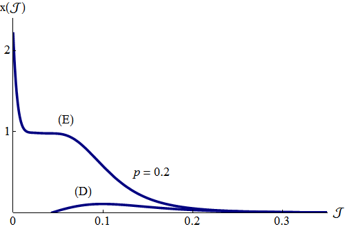
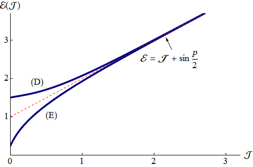
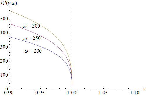
The dispersion relations (B)–(B) differ only in the signs in front of the odd-powered exponential corrections. In figure 7 we have plotted $x\left(p=0.2,\mathcal{J}\right)$ (left) and $\mathcal{E}\left(p=3.0,\mathcal{J}\right)$ (right), by using formulae (B)–(B) of the current section. The plot of $x=x\left(\mathcal{J}\right)$ on the left also includes formula $x\left(p=0.2,\mathcal{J}\right)$ that corresponds to the doubled region of the GM. We shall henceforth label the curves in the elementary region with an (E) and the curves in the doubled region with a (D). Our approximations are of course more trustworthy as the scaled angular momentum $\mathcal{J}$ gets larger and the infinite-volume HM result (A.6) is retrieved.
Single spikes are a little different from giant magnons. We may understand this qualitatively by comparing the plots in figures 2 and 5. In the former, the energy $\mathcal{E}$ and the spin $\mathcal{J}$ are divergent for $\omega=1$, while the linear momentum $p$ always stays finite and less than $\pi$. In the latter, it is the energy $\mathcal{E}$ and the momentum $p$ that diverge for $v=1$, while the spin $\mathcal{J}$ is finite and less than $1$. This type of behavior signals a different dispersion relation, a different form for the corresponding finite-size corrections and demands a rather modified inversion technique. More has been said in §3.2. Setting

R ≡1J2- 1(p + 2arcsinJ)(p + q)⋅cotq2J ≡sinq2(B.24)R ≡1superscriptJ2- 1p + 2arcsinJp + q⋅cotq2J ≡sinq2missing-subexpression(B.24)\halign to=0.0pt{\relax\global\advance\@IEEEeqncolcnt by 1\relax\begingroup\csname @IEEEeqnarraycolPREl\endcsname#\relax\relax\relax\relax\relax\relax\relax\relax\relax\relax\csname @IEEEeqnarraycolPOSTl\endcsname\relax\relax\relax\relax\relax\relax\relax\relax\relax\relax\endgroup&\relax\global\advance\@IEEEeqncolcnt by 1\relax\begingroup\csname @IEEEeqnarraycolPREl\endcsname#\relax\relax\relax\relax\relax\relax\relax\relax\relax\relax\csname @IEEEeqnarraycolPOSTl\endcsname\relax\relax\relax\relax\relax\relax\relax\relax\relax\relax\endgroup&\global\advance\@IEEEeqncolcnt by 1\relax\bgroup#\egroup&\global\advance\@IEEEeqncolcnt by 1\relax\hbox to\z@\bgroup\hss#\egroup\cr$\displaystyle\mathcal{R} \equiv\sqrt{\frac{1}{\mathcal{J}^{2}} - 1} \cdot\left(p + 2\arcsin\mathcal{J}\right) = \left(p + q\right)\cdot\cot\frac{q}{2}\,, \quad\mathcal{J} \equiv\sin\frac{q}{2}, $\hfil&$\displaystyle$\hfil&{\vrule width=0.0pt,height=0.0pt,depth=0.0pt}&0.0pt{\hss{\normalcolor(B.24)}}\cr}

the following results are obtained.
$\bullet$ Finite-Size Single Spikes: Elementary Region,  $0\leq 1/\omega<\left|v\right|\leq 1$.

E - p2q2+ 4sin2q2tanq2⋅e-R{8p2cos2q2+ 2pcosq2(8qcosq2- sin3q2+ 7sinq2)+ 8q2cos2q2- 2qsinq (cosq - (B.25)- 3) + sin2q2(cos2q - 2cosq + 5)}sec2q2tanq2⋅e-2R{32p4cos4q28p33cos3q2(48qcosq2- 11sin3q2(B.26)+ 25sinq2) + p2cos2q2[192q2cos2q2- 8qsinq(11cosq - 7)- 5cos3q + 22cos2q - 59cosq + 42] + (B.27)14pcosq2[512q3cos3q2- 32q2sinq   cosq2(11cosq - 7)+ 16q sinq   sinq2(5cos2q - 12cosq + 15)- 8sin3q2(B.28)(cos3q - 5cos2q + 15cosq - 27)] + 32q4cos4q283q3cos2q2sinq (11cosq - 7)+ q2sin2q(5cos2q - (B.29)12cosq + 15) - qsinq sin2q2(cos3q - 5cos2q + 15cosq - 27)16sin4q2(cos4q + 2cos3q + 16cos2q - (B.30)- 50cosq + 127)} cscq2sec5q2⋅e-3R+ … (B.31)E - p2q2superscript+ 4sin2q2tanq2superscript⋅e-Rsuperscript{8p2superscriptcos2q2+ 2pcosq28qcosq2- sin3q2+ 7sinq2superscript+ 8q2superscriptcos2q2- 2qsinq (cosq - (B.25)missing-subexpressionsuperscript- 3) + sin2q2cos2q - 2cosq + 5superscript}sec2q2tanq2superscript⋅e-2Rsuperscript{32p4superscriptcos4q2superscript8p33superscriptcos3q2(48qcosq2- 11sin3q2(B.26)missing-subexpression+ 25sinq2superscript) + p2superscriptcos2q2superscript[192q2superscriptcos2q2- 8qsinq11cosq - 7- 5cos3q + 22cos2q - 59cosq + 42] + (B.27)missing-subexpression14pcosq2superscript[512q3superscriptcos3q2superscript- 32q2sinq   cosq211cosq - 7+ 16q sinq   sinq25cos2q - 12cosq + 15superscript- 8sin3q2(B.28)missing-subexpressioncos3q - 5cos2q + 15cosq - 27superscript] + 32q4superscriptcos4q283superscriptq3superscriptcos2q2sinq 11cosq - 7superscript+ q2superscriptsin2q(5cos2q - (B.29)missing-subexpressionsuperscript12cosq + 15) - qsinq sin2q2cos3q - 5cos2q + 15cosq - 2716superscriptsin4q2(cos4q + 2cos3q + 16cos2q - (B.30)missing-subexpression- 50cosq + 127)} cscq2superscriptsec5q2superscript⋅e-3R+ … (B.31)\halign to=0.0pt{\relax\global\advance\@IEEEeqncolcnt by 1\relax\begingroup\csname @IEEEeqnarraycolPREl\endcsname#\relax\relax\relax\relax\relax\relax\relax\relax\relax\relax\csname @IEEEeqnarraycolPOSTl\endcsname\relax\relax\relax\relax\relax\relax\relax\relax\relax\relax\endgroup&\relax\global\advance\@IEEEeqncolcnt by 1\relax\begingroup\csname @IEEEeqnarraycolPREl\endcsname#\relax\relax\relax\relax\relax\relax\relax\relax\relax\relax\csname @IEEEeqnarraycolPOSTl\endcsname\relax\relax\relax\relax\relax\relax\relax\relax\relax\relax\endgroup&\global\advance\@IEEEeqncolcnt by 1\relax\bgroup#\egroup&\global\advance\@IEEEeqncolcnt by 1\relax\hbox to\z@\bgroup\hss#\egroup\cr$\displaystyle\mathcal{E} - \frac{p}{2} = \frac{q}{2} $\hfil&$\displaystyle{\color[rgb]{1,0,0}+} 4\sin^{2}\frac{q}{2}\tan\frac{q}{2}\cdot e^{-\mathcal{R}} + \Bigg{\{}8p^{2}\cos^{2}\frac{q}{2} + 2p\cos\frac{q}{2} \left(8q\cos\frac{q}{2} - \sin\frac{3q}{2} + 7\sin\frac{q}{2}\right) + 8q^{2}\cos^{2}\frac{q}{2} - 2q\sin q \big{(}\cos q - $\hfil&{{}\vrule width=0.0pt,height=0.0pt,depth=0.0pt}&0.0pt{\hss{\normalcolor(B.25)}}\cr\penalty 0\vskip 3.0pt\vskip 12.0pt\cr$\displaystyle$\hfil&$\displaystyle- 3\big{)} + \sin^{2}\frac{q}{2}\left(\cos 2q -{\color[rgb]{1,0,0} 2\cos q + 5}\right)\Bigg{\}}\sec^{2}\frac{q}{2}\tan\frac{q}{2} \cdot e^{-2\mathcal{R}} + \Bigg{\{}32p^{4}\cos^{4}\frac{q}{2} + \frac{8p^{3}}{3}\cos^{3}\frac{q}{2}\Big{(}48q\cos\frac{q}{2} - 11\sin\frac{3q}{2} + $\hfil&{{}\vrule width=0.0pt,height=0.0pt,depth=0.0pt}&0.0pt{\hss{\normalcolor(B.26)}}\cr\penalty 0\vskip 3.0pt\vskip 12.0pt\cr$\displaystyle$\hfil&$\displaystyle+ 25\sin\frac{q}{2}\Big{)} + p^{2}\cos^{2}\frac{q}{2}\bigg{[}192q^{2}\cos^{2}\frac{q}{2} - 8q\sin q\left(11\cos q - 7\right) - 5\cos 3q + {\color[rgb]{1,0,0}22\cos 2q - 59\cos q + 42}\bigg{]} + $\hfil&{{}\vrule width=0.0pt,height=0.0pt,depth=0.0pt}&0.0pt{\hss{\normalcolor(B.27)}}\cr\penalty 0\vskip 3.0pt\vskip 12.0pt\cr$\displaystyle$\hfil&$\displaystyle+ \frac{1}{4}p\cos\frac{q}{2}\bigg{[}512q^{3}\cos^{3}\frac{q}{2} - 32q^{2}\sin q \, \cos\frac{q}{2} \left(11\cos q - 7\right) + 16q \sin q \, \sin\frac{q}{2}\left(5\cos 2q - {\color[rgb]{1,0,0}12\cos q + 15}\right) - 8\sin^{3}\frac{q}{2}\cdot$\hfil&{{}\vrule width=0.0pt,height=0.0pt,depth=0.0pt}&0.0pt{\hss{\normalcolor(B.28)}}\cr\penalty 0\vskip 3.0pt\vskip 12.0pt\cr$\displaystyle$\hfil&$\displaystyle\cdot\left(\cos 3q - {\color[rgb]{1,0,0}5\cos 2q + 15\cos q - 27}\right)\bigg{]} + 32q^{4}\cos^{4}\frac{q}{2} - \frac{8}{3}q^{3} \cos^{2}\frac{q}{2} \sin q \left(11\cos q - 7\right) + q^{2}\sin^{2}q\big{(}5\cos 2q - $\hfil&{{}\vrule width=0.0pt,height=0.0pt,depth=0.0pt}&0.0pt{\hss{\normalcolor(B.29)}}\cr\penalty 0\vskip 3.0pt\vskip 12.0pt\cr$\displaystyle$\hfil&$\displaystyle- {\color[rgb]{1,0,0}12\cos q + 15}\big{)} - q\sin q \sin^{2}\frac{q}{2}\left(\cos 3q - {\color[rgb]{1,0,0}5\cos 2q + 15\cos q - 27}\right) + \frac{1}{6} \sin^{4}\frac{q}{2}\big{(}\cos 4q {\color[rgb]{1,0,0}+ 2\cos 3q + 16\cos 2q - }$\hfil&{{}\vrule width=0.0pt,height=0.0pt,depth=0.0pt}&0.0pt{\hss{\normalcolor(B.30)}}\cr\penalty 0\vskip 3.0pt\vskip 12.0pt\cr$\displaystyle$\hfil&$\displaystyle{\color[rgb]{1,0,0}- 50\cos q + 127}\big{)}\Bigg{\}} \csc\frac{q}{2}\sec^{5}\frac{q}{2} \cdot e^{-3\mathcal{R}} + \ldots $\hfil&{\vrule width=0.0pt,height=0.0pt,depth=0.0pt}&0.0pt{\hss{\normalcolor(B.31)}}\cr}

Refer to caption
Refer to caption
Figure 8: Inverse spin function and energy of finite-size single spikes, (B)–(B).

$\bullet$ Finite-Size Single Spikes: Doubled Region,  $0\leq 1/\omega\leq 1\leq\left|v\right|$.

E - p2q2- 4sin2q2tanq2⋅e-R{8p2cos2q2+ 2pcosq2(8qcosq2- sin3q2+ 7sinq2)+ 8q2cos2q2- 2qsinq (cosq - (B.32)- 3) + sin2q2(cos2q - 34cosq - 91 + 64csc2q2)}sec2q2tanq2⋅e-2R- {32p4cos4q28p33cos3q2(48qcosq2(B.33)- 11sin3q2+ 25sinq2) + p2cos2q2[192q2cos2q2- 8qsinq(11cosq - 7)- 5cos3q +  86cos2q + 197cosq + (B.34)+ 234] + 14pcosq2[512q3cos3q2- 32q2sinq   cosq2(11cosq - 7)+ 16q sinq   sinq2(5cos2q - 76cosq - 177 + (B.35) + 128csc2q2) - 8sin3q2(cos3q - 69cos2q - 433cosq - 795 + 384csc2q2)] + 32q4cos4q283q3cos2q2sinq (B.36)(11cosq - 7)+ q2sin2q(5cos2q - 76cosq - 177 + 128csc2q2)- qsinq sin2q2(cos3q - 69cos2q - 433cosq(B.37) - 795 + 384csc2q2) + 16sin4q2(cos4q - 190cos3q - 1424cos2q - 4466cosq - 3809 + 768csc2q2)} cscq2(B.38)⋅sec5q2⋅e-3R+ … (B.39)E - p2q2superscript- 4sin2q2tanq2superscript⋅e-Rsuperscript{8p2superscriptcos2q2+ 2pcosq28qcosq2- sin3q2+ 7sinq2superscript+ 8q2superscriptcos2q2- 2qsinq (cosq - (B.32)missing-subexpressionsuperscript- 3) + sin2q2superscriptcos2q - 34cosq - 91 + 64csc2q2superscript}sec2q2tanq2superscript⋅e-2Rsuperscript- {32p4superscriptcos4q2superscript8p33superscriptcos3q2(48qcosq2(B.33)missing-subexpression- 11sin3q2+ 25sinq2superscript) + p2superscriptcos2q2superscript[192q2superscriptcos2q2- 8qsinq11cosq - 7- 5cos3q +  86cos2q + 197cosq + (B.34)missing-subexpression+ 234] + 14pcosq2superscript[512q3superscriptcos3q2superscript- 32q2sinq   cosq211cosq - 7+ 16q sinq   sinq2(5cos2q - 76cosq - 177 + (B.35)missing-subexpressionsuperscript + 128csc2q2superscript) - 8sin3q2superscriptcos3q - 69cos2q - 433cosq - 795 + 384csc2q2superscript] + 32q4superscriptcos4q283superscriptq3superscriptcos2q2sinq (B.36)missing-subexpression11cosq - 7superscript+ q2superscriptsin2qsuperscript5cos2q - 76cosq - 177 + 128csc2q2superscript- qsinq sin2q2(cos3q - 69cos2q - 433cosq(B.37)missing-subexpressionsuperscript - 795 + 384csc2q2) + 16superscriptsin4q2superscript(cos4q - 190cos3q - 1424cos2q - 4466cosq - 3809 + 768csc2q2)} cscq2(B.38)missing-subexpressionsuperscript⋅sec5q2superscript⋅e-3R+ … (B.39)\halign to=0.0pt{\relax\global\advance\@IEEEeqncolcnt by 1\relax\begingroup\csname @IEEEeqnarraycolPREl\endcsname#\relax\relax\relax\relax\relax\relax\relax\relax\relax\relax\csname @IEEEeqnarraycolPOSTl\endcsname\relax\relax\relax\relax\relax\relax\relax\relax\relax\relax\endgroup&\relax\global\advance\@IEEEeqncolcnt by 1\relax\begingroup\csname @IEEEeqnarraycolPREl\endcsname#\relax\relax\relax\relax\relax\relax\relax\relax\relax\relax\csname @IEEEeqnarraycolPOSTl\endcsname\relax\relax\relax\relax\relax\relax\relax\relax\relax\relax\endgroup&\global\advance\@IEEEeqncolcnt by 1\relax\bgroup#\egroup&\global\advance\@IEEEeqncolcnt by 1\relax\hbox to\z@\bgroup\hss#\egroup\cr$\displaystyle\mathcal{E} - \frac{p}{2} = \frac{q}{2} $\hfil&$\displaystyle{\color[rgb]{1,0,0}-} 4\sin^{2}\frac{q}{2}\tan\frac{q}{2}\cdot e^{-\mathcal{R}} + \Bigg{\{}8p^{2}\cos^{2}\frac{q}{2} + 2p\cos\frac{q}{2} \left(8q\cos\frac{q}{2} - \sin\frac{3q}{2} + 7\sin\frac{q}{2}\right) + 8q^{2}\cos^{2}\frac{q}{2} - 2q\sin q \big{(}\cos q - $\hfil&{{}\vrule width=0.0pt,height=0.0pt,depth=0.0pt}&0.0pt{\hss{\normalcolor(B.32)}}\cr\penalty 0\vskip 3.0pt\vskip 12.0pt\cr$\displaystyle$\hfil&$\displaystyle- 3\big{)} + \sin^{2}\frac{q}{2}\left(\cos 2q -{\color[rgb]{1,0,0} 34\cos q - 91 + 64\csc^{2}\frac{q}{2}}\right)\Bigg{\}}\sec^{2}\frac{q}{2}\tan\frac{q}{2} \cdot e^{-2\mathcal{R}} {\color[rgb]{1,0,0}-} \Bigg{\{}32p^{4}\cos^{4}\frac{q}{2} + \frac{8p^{3}}{3}\cos^{3}\frac{q}{2}\Big{(}48q\cos\frac{q}{2} $\hfil&{{}\vrule width=0.0pt,height=0.0pt,depth=0.0pt}&0.0pt{\hss{\normalcolor(B.33)}}\cr\penalty 0\vskip 3.0pt\vskip 12.0pt\cr$\displaystyle$\hfil&$\displaystyle- 11\sin\frac{3q}{2} + 25\sin\frac{q}{2}\Big{)} + p^{2}\cos^{2}\frac{q}{2}\bigg{[}192q^{2}\cos^{2}\frac{q}{2} - 8q\sin q\left(11\cos q - 7\right) - 5\cos 3q + {\color[rgb]{1,0,0} 86\cos 2q + 197\cos q +} $\hfil&{{}\vrule width=0.0pt,height=0.0pt,depth=0.0pt}&0.0pt{\hss{\normalcolor(B.34)}}\cr\penalty 0\vskip 3.0pt\vskip 12.0pt\cr$\displaystyle$\hfil&$\displaystyle{\color[rgb]{1,0,0}+ 234}\bigg{]} + \frac{1}{4}p\cos\frac{q}{2}\bigg{[}512q^{3}\cos^{3}\frac{q}{2} - 32q^{2}\sin q \, \cos\frac{q}{2} \left(11\cos q - 7\right) + 16q \sin q \, \sin\frac{q}{2}\Big{(}5\cos 2q -{\color[rgb]{1,0,0} 76\cos q - 177 +} $\hfil&{{}\vrule width=0.0pt,height=0.0pt,depth=0.0pt}&0.0pt{\hss{\normalcolor(B.35)}}\cr\penalty 0\vskip 3.0pt\vskip 12.0pt\cr$\displaystyle$\hfil&$\displaystyle{\color[rgb]{1,0,0} + 128\csc^{2}\frac{q}{2}}\Big{)} - 8\sin^{3}\frac{q}{2}\cdot\left(\cos 3q -{\color[rgb]{1,0,0} 69\cos 2q - 433\cos q - 795 + 384\csc^{2}\frac{q}{2}}\right)\bigg{]} + 32q^{4}\cos^{4}\frac{q}{2} - \frac{8}{3}q^{3} \cos^{2}\frac{q}{2} \sin q $\hfil&{{}\vrule width=0.0pt,height=0.0pt,depth=0.0pt}&0.0pt{\hss{\normalcolor(B.36)}}\cr\penalty 0\vskip 3.0pt\vskip 12.0pt\cr$\displaystyle$\hfil&$\displaystyle\cdot\left(11\cos q - 7\right) + q^{2}\sin^{2}q\left(5\cos 2q -{\color[rgb]{1,0,0} 76\cos q - 177 + 128\csc^{2}\frac{q}{2}}\right) - q\sin q \sin^{2}\frac{q}{2}\Big{(}\cos 3q -{\color[rgb]{1,0,0} 69\cos 2q - 433\cos q}$\hfil&{{}\vrule width=0.0pt,height=0.0pt,depth=0.0pt}&0.0pt{\hss{\normalcolor(B.37)}}\cr\penalty 0\vskip 3.0pt\vskip 12.0pt\cr$\displaystyle$\hfil&$\displaystyle{\color[rgb]{1,0,0} - 795 + 384\csc^{2}\frac{q}{2}}\Big{)} + \frac{1}{6} \sin^{4}\frac{q}{2}\big{(}\cos 4q {\color[rgb]{1,0,0}- 190\cos 3q - 1424\cos 2q - 4466\cos q - 3809 + 768\csc^{2}\frac{q}{2}}\big{)}\Bigg{\}} \csc\frac{q}{2}\cdot$\hfil&{{}\vrule width=0.0pt,height=0.0pt,depth=0.0pt}&0.0pt{\hss{\normalcolor(B.38)}}\cr\penalty 0\vskip 3.0pt\vskip 12.0pt\cr$\displaystyle$\hfil&$\displaystyle\cdot\sec^{5}\frac{q}{2} \cdot e^{-3\mathcal{R}} + \ldots $\hfil&{\vrule width=0.0pt,height=0.0pt,depth=0.0pt}&0.0pt{\hss{\normalcolor(B.39)}}\cr}

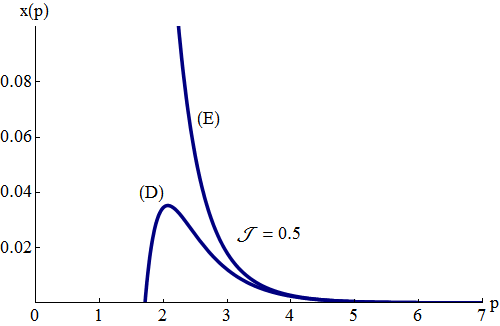
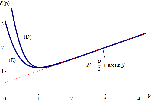
As before, different terms between the two formulas (B)–(B) are in red color. The plots $x\left(p,\mathcal{J}=0.5\right)$ (left) and $\mathcal{E}\left(p,\mathcal{J}=0.5\right)$ (right) can be found in figure 8. The latter is based on formulae (B)–(B) that give the energy of a single spike, while the former is based on formulae analogous to (B) that we have omitted. Letters (E) and (D) label the curves of the elementary and doubled regions of single spikes respectively. Again, these approximations are more trustworthy as the momentum $p$ gets larger and (A.6) is approached.

Appendix C Convergence of Large-Spin/Winding Expansions

In this appendix we discuss an issue that was brought to our attention during the peer-review process. The ultimate goal of this paper was to compute the classical spectrum of giant magnons (1) and single spikes (1) for large values of the spin $\mathcal{J}\equiv\pi J/\sqrt{\lambda}\rightarrow\infty$ and the linear momentum $p$ respectively. In the former case (1), our problem is essentially equivalent to the computation of the following set of coefficients $\mathcal{A}_{mn}$:

 m →(C.1)n ↓A10A20A21A22A30A31A32A33A34A40A41A42A43A44A45A46An0An1An2An3An4An5An6Anm(C.2) m →(C.1)missing-subexpressionn ↓subscriptA10missing-subexpressionmissing-subexpressionmissing-subexpressionmissing-subexpressionmissing-subexpressionmissing-subexpressionmissing-subexpressionmissing-subexpressionmissing-subexpressionmissing-subexpressionsubscriptA20subscriptA21subscriptA22missing-subexpressionmissing-subexpressionmissing-subexpressionmissing-subexpressionmissing-subexpressionmissing-subexpressionmissing-subexpressionmissing-subexpressionsubscriptA30subscriptA31subscriptA32subscriptA33subscriptA34missing-subexpressionmissing-subexpressionmissing-subexpressionmissing-subexpressionmissing-subexpressionmissing-subexpressionsubscriptA40subscriptA41subscriptA42subscriptA43subscriptA44subscriptA45subscriptA46missing-subexpressionmissing-subexpressionmissing-subexpressionmissing-subexpressionmissing-subexpressionmissing-subexpressionmissing-subexpressionmissing-subexpressionmissing-subexpressionmissing-subexpressionmissing-subexpressionmissing-subexpressionmissing-subexpressionmissing-subexpressionsubscriptAn0subscriptAn1subscriptAn2subscriptAn3subscriptAn4subscriptAn5subscriptAn6subscriptAnmmissing-subexpressionmissing-subexpressionmissing-subexpressionmissing-subexpressionmissing-subexpressionmissing-subexpressionmissing-subexpressionmissing-subexpressionmissing-subexpressionmissing-subexpression(C.2)\halign to=0.0pt{\relax\global\advance\@IEEEeqncolcnt by 1\relax\begingroup\csname @IEEEeqnarraycolPREl\endcsname#\relax\relax\relax\relax\relax\relax\relax\relax\relax\relax\csname @IEEEeqnarraycolPOSTl\endcsname\relax\relax\relax\relax\relax\relax\relax\relax\relax\relax\endgroup&\global\advance\@IEEEeqncolcnt by 1\relax\bgroup#\egroup&\global\advance\@IEEEeqncolcnt by 1\relax\hbox to\z@\bgroup\hss#\egroup\cr$\displaystyle\hskip 28.45274pt m \rightarrow$\hfil&{{}\vrule width=0.0pt,height=0.0pt,depth=0.0pt}&0.0pt{\hss{\normalcolor(C.1)}}\cr\penalty 0\vskip 3.0pt\vskip 6.0pt\cr$\displaystyle\begin{array}[]{lcccccccccc}n \downarrow&\mathcal{A}_{10}\\[6.0pt] &\mathcal{A}_{20}&\mathcal{A}_{21}&\mathcal{A}_{22}\\[6.0pt] &\mathcal{A}_{30}&\mathcal{A}_{31}&\mathcal{A}_{32}&\mathcal{A}_{33}&\mathcal{A}_{34}\\[6.0pt] &\mathcal{A}_{40}&\mathcal{A}_{41}&\mathcal{A}_{42}&\mathcal{A}_{43}&\mathcal{A}_{44}&\mathcal{A}_{45}&\mathcal{A}_{46}\\[6.0pt] &\vdots&\\[6.0pt] &\mathcal{A}_{n0}&\mathcal{A}_{n1}&\mathcal{A}_{n2}&\mathcal{A}_{n3}&\mathcal{A}_{n4}&\mathcal{A}_{n5}&\mathcal{A}_{n6}&\ldots&\mathcal{A}_{nm}&\ldots\\[6.0pt] &\vdots&\end{array} $\hfil&{\vrule width=0.0pt,height=0.0pt,depth=0.0pt}&0.0pt{\hss{\normalcolor(C.2)}}\cr}

Because of exponential suppression $e^{-n\mathcal{L}}$ ($\mathcal{L}\equiv 2\mathcal{J}\csc p/2+2\rightarrow\infty$), the top rows are more important than the lower ones. Leftmost coefficients are multiplied by higher powers of $\mathcal{J}\rightarrow\infty$ and are more important than the coefficients on their right. E.g. $\mathcal{A}_{21}$ is far more important than all the coefficients on its right and below it. Therefore, one may question the usefulness of the Lambert function expressions (2.3)–(3.1), which essentially sum each of the first three exponentially suppressed columns of (C).
To answer this type of criticism, remember that AdS/CFT is an exact duality. It is not enough to say that e.g. some string state energies are approximately equal to the scaling dimensions of some gauge theory operators, or that certain Lüscher-type corrections reproduce part of the string spectrum. If one term is missing, then something is not correct with our model and we have a problem. In an experimental situation, we are usually interested only in the dominant part of some theoretical prediction, because this is what we can measure. This is not so with theory. We have to match all the terms in order to prove that two theories are the same.
Therefore, in an exact duality framework, the absolute matching of both dominant and subdominant terms is required. In this sense, the exponential corrections are equally important with the power-law corrections.
In addition, let us note that the W-function expressions contain new information in the form of terms that are completely impossible to obtain by means of a computer or otherwise. For the present, it also seems very hard to perform any kind of summation that respects the hierarchy of (C) by proceeding first along the rows of (C) and then along its columns.
The same considerations also apply to the case of single spikes. However, because the dispersion relations of single spikes are exponentially suppressed by the factor $e^{-n\mathcal{R}}\rightarrow 0$, where

R ≡1J2- 1(p + 2arcsinJ)(p + q)⋅cotq2J ≡sinq2(C.3)R ≡1superscriptJ2- 1p + 2arcsinJp + q⋅cotq2J ≡sinq2missing-subexpression(C.3)\halign to=0.0pt{\relax\global\advance\@IEEEeqncolcnt by 1\relax\begingroup\csname @IEEEeqnarraycolPREl\endcsname#\relax\relax\relax\relax\relax\relax\relax\relax\relax\relax\csname @IEEEeqnarraycolPOSTl\endcsname\relax\relax\relax\relax\relax\relax\relax\relax\relax\relax\endgroup&\relax\global\advance\@IEEEeqncolcnt by 1\relax\begingroup\csname @IEEEeqnarraycolPREl\endcsname#\relax\relax\relax\relax\relax\relax\relax\relax\relax\relax\csname @IEEEeqnarraycolPOSTl\endcsname\relax\relax\relax\relax\relax\relax\relax\relax\relax\relax\endgroup&\global\advance\@IEEEeqncolcnt by 1\relax\bgroup#\egroup&\global\advance\@IEEEeqncolcnt by 1\relax\hbox to\z@\bgroup\hss#\egroup\cr$\displaystyle\mathcal{R} \equiv\sqrt{\frac{1}{\mathcal{J}^{2}} - 1} \cdot\left(p + 2\arcsin\mathcal{J}\right) = \left(p + q\right)\cdot\cot\frac{q}{2}\,, \quad\mathcal{J} \equiv\sin\frac{q}{2}, $\hfil&$\displaystyle$\hfil&{\vrule width=0.0pt,height=0.0pt,depth=0.0pt}&0.0pt{\hss{\normalcolor(C.3)}}\cr}

it seems that for $\mathcal{J}=1$, $\mathcal{R}$ becomes finite and the exponential suppression disappears. In fact, the single spike dispersion relations (B)–(B) diverge if we first consider the limit $\mathcal{J}=1$ and then the limit $p=\infty$.151515As a side remark, note also that many of the trigonometric coefficients of (B)–(B) blow up in the limit $\mathcal{J}=1\Leftrightarrow q=\pi$, implying that the value $\mathcal{J}=1$ is singular. It is also clear from the right plot of figure 5 that for $\omega=\infty$, $\mathcal{J}$ approaches unity from above ($\mathcal{J}\rightarrow 1^{+}$) and $\mathcal{R}$ in (C) becomes complex.

Refer to caption
Refer to caption
Figure 9: Behavior of $\mathcal{R}$ near $v=1$, for various values of the angular velocity $\omega$.

First of all, let us see why finite values of the coefficient $\mathcal{R}$ cannot possibly be accepted in the dispersion relations (B)–(B). As in the case of giant magnons (for which $\omega\rightarrow 1$), the finite-size corrections to the dispersion relation of single spikes are computed in the infinite-size regime

v →1   &   x ≡1 - v21 - 1/ω2→0, (C.4)v →1   &   x ≡superscript1 - v2superscript1 - 1/ω2→0, missing-subexpression(C.4)\halign to=0.0pt{\relax\global\advance\@IEEEeqncolcnt by 1\relax\begingroup\csname @IEEEeqnarraycolPREl\endcsname#\relax\relax\relax\relax\relax\relax\relax\relax\relax\relax\csname @IEEEeqnarraycolPOSTl\endcsname\relax\relax\relax\relax\relax\relax\relax\relax\relax\relax\endgroup&\relax\global\advance\@IEEEeqncolcnt by 1\relax\begingroup\csname @IEEEeqnarraycolPREl\endcsname#\relax\relax\relax\relax\relax\relax\relax\relax\relax\relax\csname @IEEEeqnarraycolPOSTl\endcsname\relax\relax\relax\relax\relax\relax\relax\relax\relax\relax\endgroup&\global\advance\@IEEEeqncolcnt by 1\relax\bgroup#\egroup&\global\advance\@IEEEeqncolcnt by 1\relax\hbox to\z@\bgroup\hss#\egroup\cr$\displaystyle v \rightarrow 1 \qquad\& \qquad x \equiv\frac{1 - v^{2}}{1 - 1/\omega^{2}} \rightarrow 0, $\hfil&$\displaystyle$\hfil&{\vrule width=0.0pt,height=0.0pt,depth=0.0pt}&0.0pt{\hss{\normalcolor(C.4)}}\cr}

which puts a constraint upon all the possible values of the inverse momentum $x$. For single spikes in the elementary/doubled region, the first few terms of the inverse momentum function are given by:

x = 16e-R(±64p2csc2q2+ …)e-2R+ …= ±4p2sin2q2⋅W(±4 p2csc2q2e-R)+ … (C.5)superscriptx = 16e-Rsuperscript±64p2superscriptcsc2q2+ …superscripte-2R+ …= ±4superscriptp2superscriptsin2q2⋅Wsuperscript±4 p2superscriptcsc2q2superscripte-R+ … missing-subexpression(C.5)\halign to=0.0pt{\relax\global\advance\@IEEEeqncolcnt by 1\relax\begingroup\csname @IEEEeqnarraycolPREl\endcsname#\relax\relax\relax\relax\relax\relax\relax\relax\relax\relax\csname @IEEEeqnarraycolPOSTl\endcsname\relax\relax\relax\relax\relax\relax\relax\relax\relax\relax\endgroup&\relax\global\advance\@IEEEeqncolcnt by 1\relax\begingroup\csname @IEEEeqnarraycolPREl\endcsname#\relax\relax\relax\relax\relax\relax\relax\relax\relax\relax\csname @IEEEeqnarraycolPOSTl\endcsname\relax\relax\relax\relax\relax\relax\relax\relax\relax\relax\endgroup&\global\advance\@IEEEeqncolcnt by 1\relax\bgroup#\egroup&\global\advance\@IEEEeqncolcnt by 1\relax\hbox to\z@\bgroup\hss#\egroup\cr$\displaystyle x = 16e^{-\mathcal{R}} - \left(\pm 64p^{2} \csc^{2}\frac{q}{2} + \ldots\right)e^{-2\mathcal{R}} + \ldots= \pm\frac{4}{p^{2}}\sin^{2}\frac{q}{2}\cdot W\left(\pm 4 p^{2} \csc^{2}\frac{q}{2} e^{-\mathcal{R}}\right) + \ldots\qquad$\hfil&$\displaystyle$\hfil&{\vrule width=0.0pt,height=0.0pt,depth=0.0pt}&0.0pt{\hss{\normalcolor(C.5)}}\cr}

where the minus sign refers to the elementary161616Note also the constraint $4p^{2}\csc^{2}\left(q/2\right)e^{-\mathcal{R}}\leq e^{-1}$, imposed to the argument of the W-function in the elementary region by the corresponding branch cut. and the plus sign refers to the doubled region of single spikes. Without the exponential suppression $e^{-\mathcal{R}}\rightarrow 0$, the inverse momentum $x$ does not have the desired behavior $x\rightarrow 0$ as $p\rightarrow\infty$. Therefore the dispersion relations of single spikes (B)–(B) are only valid if

R ≫1   &   p ≫1. (C.6)R ≫1   &   p ≫1. missing-subexpression(C.6)\halign to=0.0pt{\relax\global\advance\@IEEEeqncolcnt by 1\relax\begingroup\csname @IEEEeqnarraycolPREl\endcsname#\relax\relax\relax\relax\relax\relax\relax\relax\relax\relax\csname @IEEEeqnarraycolPOSTl\endcsname\relax\relax\relax\relax\relax\relax\relax\relax\relax\relax\endgroup&\relax\global\advance\@IEEEeqncolcnt by 1\relax\begingroup\csname @IEEEeqnarraycolPREl\endcsname#\relax\relax\relax\relax\relax\relax\relax\relax\relax\relax\csname @IEEEeqnarraycolPOSTl\endcsname\relax\relax\relax\relax\relax\relax\relax\relax\relax\relax\endgroup&\global\advance\@IEEEeqncolcnt by 1\relax\bgroup#\egroup&\global\advance\@IEEEeqncolcnt by 1\relax\hbox to\z@\bgroup\hss#\egroup\cr$\displaystyle\mathcal{R} \gg 1 \qquad\& \qquad p \gg 1. $\hfil&$\displaystyle$\hfil&{\vrule width=0.0pt,height=0.0pt,depth=0.0pt}&0.0pt{\hss{\normalcolor(C.6)}}\cr}

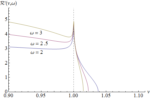
It turns out that this condition becomes less and less valid as the angular velocity $\omega$ of single spikes approaches infinity. If we define $\mathcal{R}^{\prime}$ as:

R ≡1J2- 1(p + 2arcsinJ)R’ ≡1J2- 1⋅p,  p →∞, (C.7)R ≡1superscriptJ2- 1p + 2arcsinJR’ ≡1superscriptJ2- 1⋅p,  p →∞, (C.7)\halign to=0.0pt{\relax\global\advance\@IEEEeqncolcnt by 1\relax\begingroup\csname @IEEEeqnarraycolPREl\endcsname#\relax\relax\relax\relax\relax\relax\relax\relax\relax\relax\csname @IEEEeqnarraycolPOSTl\endcsname\relax\relax\relax\relax\relax\relax\relax\relax\relax\relax\endgroup&\global\advance\@IEEEeqncolcnt by 1\relax\bgroup#\egroup&\global\advance\@IEEEeqncolcnt by 1\relax\hbox to\z@\bgroup\hss#\egroup\cr$\displaystyle\mathcal{R} \equiv\sqrt{\frac{1}{\mathcal{J}^{2}} - 1} \cdot\left(p + 2\arcsin\mathcal{J}\right) \rightarrow\mathcal{R}' \equiv\sqrt{\frac{1}{\mathcal{J}^{2}} - 1}\cdot p, \quad p \rightarrow\infty, $\hfil&{\vrule width=0.0pt,height=0.0pt,depth=0.0pt}&0.0pt{\hss{\normalcolor(C.7)}}\cr}

then $\mathcal{R}^{\prime}$ gives the behavior of the coefficient $\mathcal{R}$ in the large winding regime ($v\rightarrow 1$) where the momentum $p$ becomes infinite. In figure 9 we have plotted $\mathcal{R}^{\prime}$ near $v=1$ for various values of the angular velocity $\omega$. We can convince ourselves that there’s a delta function peak at $\left\{\omega=\infty,\ v=1,\ \mathcal{J}=1\right\}$ but, if we leave the vicinity of this point, $\mathcal{R}$ may become finite. For $v=1$ the dispersion relation of infinite-size/winding single spikes (A.6),

E - p2= arcsinJ,   v = 1 (C.8)E - p2= arcsinJ,   v = 1 (C.8)\halign to=0.0pt{\relax\global\advance\@IEEEeqncolcnt by 1\relax\begingroup\csname @IEEEeqnarraycolPREc\endcsname#\relax\relax\relax\relax\relax\relax\relax\relax\relax\relax\csname @IEEEeqnarraycolPOSTc\endcsname\relax\relax\relax\relax\relax\relax\relax\relax\relax\relax\endgroup&\global\advance\@IEEEeqncolcnt by 1\relax\bgroup#\egroup&\global\advance\@IEEEeqncolcnt by 1\relax\hbox to\z@\bgroup\hss#\egroup\cr\hfil$\displaystyle\mathcal{E} - \frac{p}{2} = \arcsin\mathcal{J}, \qquad v = 1 $\hfil&{\vrule width=0.0pt,height=0.0pt,depth=0.0pt}&0.0pt{\hss{\normalcolor(C.8)}}\cr}

is well defined in the (double) infinite-size/winding limit $\omega\rightarrow\infty\Leftrightarrow\mathcal{J}\rightarrow 1$:

E - p2π2,   v = 1, ω= ∞. (C.9)E - p2π2,   v = 1, ω= ∞. (C.9)\halign to=0.0pt{\relax\global\advance\@IEEEeqncolcnt by 1\relax\begingroup\csname @IEEEeqnarraycolPREc\endcsname#\relax\relax\relax\relax\relax\relax\relax\relax\relax\relax\csname @IEEEeqnarraycolPOSTc\endcsname\relax\relax\relax\relax\relax\relax\relax\relax\relax\relax\endgroup&\global\advance\@IEEEeqncolcnt by 1\relax\bgroup#\egroup&\global\advance\@IEEEeqncolcnt by 1\relax\hbox to\z@\bgroup\hss#\egroup\cr\hfil$\displaystyle\mathcal{E} - \frac{p}{2} = \frac{\pi}{2}, \qquad v = 1, \quad\omega= \infty. $\hfil&{\vrule width=0.0pt,height=0.0pt,depth=0.0pt}&0.0pt{\hss{\normalcolor(C.9)}}\cr}

However, for $\omega=\infty,\ v\rightarrow 1^{\pm}$ (where $\mathcal{J}\rightarrow 1^{\pm}$) neither (C) nor (B)–(B) are expected to hold. Interestingly, the limit $\omega=\infty$ is a second infinite-size/winding limit of single spikes. To prove it, consider the conserved charges (A.3), (A.3), (A.3) of elementary single spikes as $\omega\rightarrow\infty\Leftrightarrow\eta\rightarrow v^{2}$:

E = v2ω2- 1ω2- 1K(η)→v21 - v2v2ηK(v2)+ O(v2η)ηv2ω2- 1ω2- 1(C.10)J = 1 - 1ω2[E(η)1-v21-1/ω2K(η)] →E(v2)(1 - v2)K(v2)+ O(v2η)(C.11)p2ω1 - 1/ω2[K(η)Π(1 - v2ω2η)] →v1 - v2v2ηK(v2)π2+ O(v2η)(C.12)E = superscriptv2superscriptω2- 1superscriptω2- 1Kηsuperscript→v2superscript1 - v2superscriptv2ηKsuperscriptv2+ Osuperscriptv2ηηsuperscriptv2superscriptω2- 1superscriptω2- 1missing-subexpression(C.10)missing-subexpressionJ = 1 - 1superscriptω2[Eηsuperscript1-v2superscript1-1/ω2Kη] →Esuperscriptv2superscript1 - v2Ksuperscriptv2+ Osuperscriptv2ηmissing-subexpression(C.11)missing-subexpressionp2ωsuperscript1 - 1/ω2[KηΠsuperscript1 - v2superscriptω2η] →vsuperscript1 - v2superscriptv2ηKsuperscriptv2π2+ Osuperscriptv2ηmissing-subexpression(C.12)\halign to=0.0pt{\relax\global\advance\@IEEEeqncolcnt by 1\relax\begingroup\csname @IEEEeqnarraycolPREl\endcsname#\relax\relax\relax\relax\relax\relax\relax\relax\relax\relax\csname @IEEEeqnarraycolPOSTl\endcsname\relax\relax\relax\relax\relax\relax\relax\relax\relax\relax\endgroup&\relax\global\advance\@IEEEeqncolcnt by 1\relax\begingroup\csname @IEEEeqnarraycolPREl\endcsname#\relax\relax\relax\relax\relax\relax\relax\relax\relax\relax\csname @IEEEeqnarraycolPOSTl\endcsname\relax\relax\relax\relax\relax\relax\relax\relax\relax\relax\endgroup&\global\advance\@IEEEeqncolcnt by 1\relax\bgroup#\egroup&\global\advance\@IEEEeqncolcnt by 1\relax\hbox to\z@\bgroup\hss#\egroup\cr$\displaystyle\mathcal{E} = \frac{v^{2} \omega^{2} - 1}{\sqrt{\omega^{2} - 1}}\,\mathbb{K}\left(\eta\right) \rightarrow v^{2} \sqrt{\frac{1 - v^{2}}{v^{2} - \eta}}\cdot\mathbb{K}\left(v^{2}\right) + O\left(\sqrt{v^{2} - \eta}\right), \qquad\eta\equiv\frac{v^{2}\omega^{2} - 1}{\omega^{2} - 1} $\hfil&$\displaystyle{}$\hfil&{\vrule width=0.0pt,height=0.0pt,depth=0.0pt}&0.0pt{\hss{\normalcolor(C.10)}}\cr\penalty 0\vskip 3.0pt\vskip 12.0pt\cr$\displaystyle\mathcal{J} = \sqrt{1 - \frac{1}{\omega^{2}}} \, \bigg{[}\mathbb{E}\left(\eta\right) - \frac{1-v^{2}}{1-1/\omega^{2}}\,\mathbb{K}\left(\eta\right)\bigg{]} \rightarrow\mathbb{E}\left(v^{2}\right) - \left(1 - v^{2}\right)\mathbb{K}\left(v^{2}\right) + O\left(v^{2} - \eta\right) $\hfil&$\displaystyle{}$\hfil&{\vrule width=0.0pt,height=0.0pt,depth=0.0pt}&0.0pt{\hss{\normalcolor(C.11)}}\cr\penalty 0\vskip 3.0pt\vskip 12.0pt\cr$\displaystyle\frac{p}{2} = \frac{v \omega}{\sqrt{1 - 1/\omega^{2}}} \, \Big{[}\mathbb{K}\left(\eta\right) - \boldsymbol{\Pi}\left(1 - v^{2}\omega^{2} ; \eta\right)\Big{]} \rightarrow v\sqrt{\frac{1 - v^{2}}{v^{2} - \eta}}\cdot\mathbb{K}\left(v^{2}\right) - \frac{\pi}{2} + O\left(\sqrt{v^{2} - \eta}\right). $\hfil&$\displaystyle$\hfil&{\vrule width=0.0pt,height=0.0pt,depth=0.0pt}&0.0pt{\hss{\normalcolor(C.12)}}\cr}

Clearly $\mathcal{E},\,p=\infty$ when $\eta=v^{2}$. To obtain $\mathcal{J}\rightarrow 1$ we must further set $v\rightarrow 1$. In the doubled region of single spikes the proof proceeds along the same lines. Now, it easy to show that the $\omega=\infty$ dispersion relation of (both elementary and doubled) infinite-size/winding single spikes is the following:

E = (p2π2)⋅v(J)ω= ∞, (C.13)E = p2π2⋅vJω= ∞, missing-subexpression(C.13)\halign to=0.0pt{\relax\global\advance\@IEEEeqncolcnt by 1\relax\begingroup\csname @IEEEeqnarraycolPREl\endcsname#\relax\relax\relax\relax\relax\relax\relax\relax\relax\relax\csname @IEEEeqnarraycolPOSTl\endcsname\relax\relax\relax\relax\relax\relax\relax\relax\relax\relax\endgroup&\relax\global\advance\@IEEEeqncolcnt by 1\relax\begingroup\csname @IEEEeqnarraycolPREl\endcsname#\relax\relax\relax\relax\relax\relax\relax\relax\relax\relax\csname @IEEEeqnarraycolPOSTl\endcsname\relax\relax\relax\relax\relax\relax\relax\relax\relax\relax\endgroup&\global\advance\@IEEEeqncolcnt by 1\relax\bgroup#\egroup&\global\advance\@IEEEeqncolcnt by 1\relax\hbox to\z@\bgroup\hss#\egroup\cr$\displaystyle\mathcal{E} = \left(\frac{p}{2} + \frac{\pi}{2}\right)\cdot v\left(\mathcal{J}\right), \qquad\omega= \infty, $\hfil&$\displaystyle$\hfil&{\vrule width=0.0pt,height=0.0pt,depth=0.0pt}&0.0pt{\hss{\normalcolor(C.13)}}\cr}

where $v\left(\mathcal{J}\right)$ gives the string’s velocity in terms of its spin. It would be interesting to study more closely the $\omega$-infinity limit of single spikes and calculate the corresponding finite-size corrections.

Appendix D Bound States & Scattering

D.1 Scattering

In this appendix we shall briefly revisit the computation of the semiclassical scattering phase-shifts of (infinite-size) giant magnons and single spikes. The giant magnon phase-shift was calculated by Hofman and Maldacena in [4] by considering the kink-antikink solution of the corresponding (via the Pohlmeyer reduction) sine-Gordon equation. The result for the scattering between two giant magnons of linear momenta $p_{1}$ and $p_{2}$ is:

δ12λπ{(cosp22- cosp12)log[1 - cosp1- p221 - cosp1+ p22]- p1sinp12}(D.1)subscriptδ12λπcossubscriptp22- cossubscriptp12logdelimited-[]1 - cossubscriptp1subscript- p221 - cossubscriptp1subscript+ p22subscript- p1sinsubscriptp12(D.1)\halign to=0.0pt{\relax\global\advance\@IEEEeqncolcnt by 1\relax\begingroup\csname @IEEEeqnarraycolPREc\endcsname#\relax\relax\relax\relax\relax\relax\relax\relax\relax\relax\csname @IEEEeqnarraycolPOSTc\endcsname\relax\relax\relax\relax\relax\relax\relax\relax\relax\relax\endgroup&\global\advance\@IEEEeqncolcnt by 1\relax\bgroup#\egroup&\global\advance\@IEEEeqncolcnt by 1\relax\hbox to\z@\bgroup\hss#\egroup\cr\hfil$\displaystyle\delta_{12} = \frac{\sqrt{\lambda}}{\pi}\left\{\left(\cos\frac{p_{2}}{2} - \cos\frac{p_{1}}{2}\right)\log\left[\frac{1 - \cos\frac{p_{1} - p_{2}}{2}}{1 - \cos\frac{p_{1} + p_{2}}{2}}\right] - p_{1} \sin\frac{p_{1}}{2}\right\}. $\hfil&{\vrule width=0.0pt,height=0.0pt,depth=0.0pt}&0.0pt{\hss{\normalcolor(D.1)}}\cr}

The presence of the last term in (D.1) depends on the choice of the worldsheet gauge and the definition of the worldsheet variable $\sigma$. It may be omitted, so that for $\sin p_{1,2}/2>0$ the phase-shift becomes,

δ(p1,p2)= -λπ(cosp12- cosp22)log[sin2p1- p24sin2p1+ p24](D.2)δsubscriptp1subscript,p2= -λπcossubscriptp12- cossubscriptp22logdelimited-[]superscriptsin2subscriptp1subscript- p24superscriptsin2subscriptp1subscript+ p24(D.2)\halign to=0.0pt{\relax\global\advance\@IEEEeqncolcnt by 1\relax\begingroup\csname @IEEEeqnarraycolPREc\endcsname#\relax\relax\relax\relax\relax\relax\relax\relax\relax\relax\csname @IEEEeqnarraycolPOSTc\endcsname\relax\relax\relax\relax\relax\relax\relax\relax\relax\relax\endgroup&\global\advance\@IEEEeqncolcnt by 1\relax\bgroup#\egroup&\global\advance\@IEEEeqncolcnt by 1\relax\hbox to\z@\bgroup\hss#\egroup\cr\hfil$\displaystyle\delta\left(p_{1},p_{2}\right) = -\frac{\sqrt{\lambda}}{\pi}\left(\cos\frac{p_{1}}{2} - \cos\frac{p_{2}}{2}\right)\log\left[\frac{\sin^{2}\frac{p_{1} - p_{2}}{4}}{\sin^{2}\frac{p_{1} + p_{2}}{4}}\right]. $\hfil&{\vrule width=0.0pt,height=0.0pt,depth=0.0pt}&0.0pt{\hss{\normalcolor(D.2)}}\cr}

This phase-shift is equal to the 2-magnon, strong-coupling ”dressing phase” $\sigma_{12(\text{AFS})}^{2}=e^{i\delta_{12}}$ that was proposed by Arutyunov, Frolov and Staudacher (AFS) in [56] as the string theory-complement of the $\mathfrak{su}\left(2\right)$, all-loop asymptotic Bethe ansatz equations of Beisert, Dippel and Staudacher (BDS) [9].
In [57] the string solution for the scattering between two giant magnons was derived by applying what is known as the dressing method171717As far as we know, this method is not in any way correlated to the dressing phase of Bethe ansätze. Their common name is only a coincidence. to a point-like string that rotates at the equator of S2. By similarly dressing the hoop string181818As we saw in appendix A, the hoop string is a motionless string that is wound around the equator of the 2-sphere with coordinates $z=0$ and $\phi=\pm\sigma+\phi_{0}$. one may write down the scattering solution between two single spikes, from which the corresponding phase-shift can be calculated. This has indeed been done in [40], leading to the result

δ(q1,q2)= -λπ{(cosq12- cosq22)log[sin2q1- q24sin2q1+ q24]- q1sinq12}(D.3)δsubscriptq1subscript,q2= -λπcossubscriptq12- cossubscriptq22logdelimited-[]superscriptsin2subscriptq1subscript- q24superscriptsin2subscriptq1subscript+ q24subscript- q1sinsubscriptq12(D.3)\halign to=0.0pt{\relax\global\advance\@IEEEeqncolcnt by 1\relax\begingroup\csname @IEEEeqnarraycolPREc\endcsname#\relax\relax\relax\relax\relax\relax\relax\relax\relax\relax\csname @IEEEeqnarraycolPOSTc\endcsname\relax\relax\relax\relax\relax\relax\relax\relax\relax\relax\endgroup&\global\advance\@IEEEeqncolcnt by 1\relax\bgroup#\egroup&\global\advance\@IEEEeqncolcnt by 1\relax\hbox to\z@\bgroup\hss#\egroup\cr\hfil$\displaystyle\delta\left(q_{1},q_{2}\right) = -\frac{\sqrt{\lambda}}{\pi}\left\{\left(\cos\frac{q_{1}}{2} - \cos\frac{q_{2}}{2}\right)\log\left[\frac{\sin^{2}\frac{q_{1} - q_{2}}{4}}{\sin^{2}\frac{q_{1} + q_{2}}{4}}\right] - q_{1} \sin\frac{q_{1}}{2}\right\}, $\hfil&{\vrule width=0.0pt,height=0.0pt,depth=0.0pt}&0.0pt{\hss{\normalcolor(D.3)}}\cr}

where $q$ is defined from $\mathcal{J}=\left(1-1/\omega^{2}\right)^{1/2}\equiv\sin q/2$ and $\omega$ and $\mathcal{J}$ are the spike’s angular velocity and conserved angular momentum respectively. Obviously, for $p\leftrightarrow q$ (D.1) agrees with the phase-shift for giant magnons (D.1) up to the non-logarithmic term $q\sin q/2$. Okamura [41] provided a qualitative explanation for the agreement between the logarithmic terms of the two formulas, by regarding single spike scattering as factorized scattering of infinitely many giant magnons.

Refer to caption
Refer to caption
Figure 10: Soliton-antisoliton scattering for giant magnons (left) and single spikes (right).

We will now provide an alternative derivation of (D.1) by $\tau\leftrightarrow\sigma$ transforming the sG solitons that correspond to giant magnons and their scattering solutions.191919This line of reasoning has been suggested in footnote 2 of [40]. As we have already explained in appendix A, the string sigma model in $\mathbb{R}\times\text{S}^{2}$ can be Pohlmeyer-reduced to the following sine-Gordon equation:

ψ¨ψ” + 12sin2ψ= 0. (D.4)¨ψψ” + 12sin2ψ= 0. missing-subexpression(D.4)\halign to=0.0pt{\relax\global\advance\@IEEEeqncolcnt by 1\relax\begingroup\csname @IEEEeqnarraycolPREl\endcsname#\relax\relax\relax\relax\relax\relax\relax\relax\relax\relax\csname @IEEEeqnarraycolPOSTl\endcsname\relax\relax\relax\relax\relax\relax\relax\relax\relax\relax\endgroup&\relax\global\advance\@IEEEeqncolcnt by 1\relax\begingroup\csname @IEEEeqnarraycolPREl\endcsname#\relax\relax\relax\relax\relax\relax\relax\relax\relax\relax\csname @IEEEeqnarraycolPOSTl\endcsname\relax\relax\relax\relax\relax\relax\relax\relax\relax\relax\endgroup&\global\advance\@IEEEeqncolcnt by 1\relax\bgroup#\egroup&\global\advance\@IEEEeqncolcnt by 1\relax\hbox to\z@\bgroup\hss#\egroup\cr$\displaystyle\ddot{\psi} - \psi'' + \frac{1}{2}\sin 2\psi= 0. $\hfil&$\displaystyle$\hfil&{\vrule width=0.0pt,height=0.0pt,depth=0.0pt}&0.0pt{\hss{\normalcolor(D.4)}}\cr}

It can be shown that (D.1) contains the following soliton-soliton scattering solution:

tanψs-s2v sinhγσcoshvγτγ11 - v2(D.5)tansubscriptψs-s2v sinhγσcoshvγτγ1superscript1 - v2(D.5)\halign to=0.0pt{\relax\global\advance\@IEEEeqncolcnt by 1\relax\begingroup\csname @IEEEeqnarraycolPREc\endcsname#\relax\relax\relax\relax\relax\relax\relax\relax\relax\relax\csname @IEEEeqnarraycolPOSTc\endcsname\relax\relax\relax\relax\relax\relax\relax\relax\relax\relax\endgroup&\global\advance\@IEEEeqncolcnt by 1\relax\bgroup#\egroup&\global\advance\@IEEEeqncolcnt by 1\relax\hbox to\z@\bgroup\hss#\egroup\cr\hfil$\displaystyle\tan\frac{\psi_{s-s}}{2} = \frac{v\,\sinh\gamma\sigma}{\cosh v\gamma\tau}\,, \quad\gamma\equiv\frac{1}{\sqrt{1 - v^{2}}}. $\hfil&{\vrule width=0.0pt,height=0.0pt,depth=0.0pt}&0.0pt{\hss{\normalcolor(D.5)}}\cr}

This solution has topological charge202020The topological charge Q is defined according to $Q=1/\pi\int_{-\infty}^{+\infty}\partial_{\sigma}\psi\,d\sigma$. $Q=+2$ and corresponds to two giant magnons that scatter in their center of mass frame. When it is $\tau\leftrightarrow\sigma$ transformed according to

τσ & ψ[π2ψ](D.6)τσ & ψdelimited-[]π2ψmissing-subexpression(D.6)\halign to=0.0pt{\relax\global\advance\@IEEEeqncolcnt by 1\relax\begingroup\csname @IEEEeqnarraycolPREl\endcsname#\relax\relax\relax\relax\relax\relax\relax\relax\relax\relax\csname @IEEEeqnarraycolPOSTl\endcsname\relax\relax\relax\relax\relax\relax\relax\relax\relax\relax\endgroup&\relax\global\advance\@IEEEeqncolcnt by 1\relax\begingroup\csname @IEEEeqnarraycolPREl\endcsname#\relax\relax\relax\relax\relax\relax\relax\relax\relax\relax\csname @IEEEeqnarraycolPOSTl\endcsname\relax\relax\relax\relax\relax\relax\relax\relax\relax\relax\endgroup&\global\advance\@IEEEeqncolcnt by 1\relax\bgroup#\egroup&\global\advance\@IEEEeqncolcnt by 1\relax\hbox to\z@\bgroup\hss#\egroup\cr$\displaystyle\tau\leftrightarrow\sigma\quad\& \quad\psi\leftrightarrow\left[\frac{\pi}{2} - \psi\right], $\hfil&$\displaystyle$\hfil&{\vrule width=0.0pt,height=0.0pt,depth=0.0pt}&0.0pt{\hss{\normalcolor(D.6)}}\cr}

the transformed solution

tanψ2coshvγσ- v sinhγτcoshvγσ+ v sinhγτ(D.7)tanψ2coshvγσ- v sinhγτcoshvγσ+ v sinhγτ(D.7)\halign to=0.0pt{\relax\global\advance\@IEEEeqncolcnt by 1\relax\begingroup\csname @IEEEeqnarraycolPREc\endcsname#\relax\relax\relax\relax\relax\relax\relax\relax\relax\relax\csname @IEEEeqnarraycolPOSTc\endcsname\relax\relax\relax\relax\relax\relax\relax\relax\relax\relax\endgroup&\global\advance\@IEEEeqncolcnt by 1\relax\bgroup#\egroup&\global\advance\@IEEEeqncolcnt by 1\relax\hbox to\z@\bgroup\hss#\egroup\cr\hfil$\displaystyle\tan\frac{\psi}{2} = \frac{\cosh v\gamma\sigma- v\,\sinh\gamma\tau}{\cosh v\gamma\sigma+ v\,\sinh\gamma\tau} $\hfil&{\vrule width=0.0pt,height=0.0pt,depth=0.0pt}&0.0pt{\hss{\normalcolor(D.7)}}\cr}

continues to satisfy (D.1) and has a topological charge of $Q=0$, that is it corresponds to soliton-antisoliton scattering. If we further set $v=1/\omega<1$, we obtain a solution of the sG equation that represents the scattering of a single spike soliton with its corresponding antisoliton:

tanψs-a2ωcoshσ/ω2- 1- sinhωτ/ω2- 1ωcoshσ/ω2- 1+ sinhωτ/ω2- 1(D.8)tansubscriptψs-a2ωcoshσ/superscriptω2- 1- sinhωτ/superscriptω2- 1ωcoshσ/superscriptω2- 1+ sinhωτ/superscriptω2- 1(D.8)\halign to=0.0pt{\relax\global\advance\@IEEEeqncolcnt by 1\relax\begingroup\csname @IEEEeqnarraycolPREc\endcsname#\relax\relax\relax\relax\relax\relax\relax\relax\relax\relax\csname @IEEEeqnarraycolPOSTc\endcsname\relax\relax\relax\relax\relax\relax\relax\relax\relax\relax\endgroup&\global\advance\@IEEEeqncolcnt by 1\relax\bgroup#\egroup&\global\advance\@IEEEeqncolcnt by 1\relax\hbox to\z@\bgroup\hss#\egroup\cr\hfil$\displaystyle\tan\frac{\psi_{s-a}}{2} = \frac{\omega\cosh\sigma/\sqrt{\omega^{2} - 1} - \sinh\omega\tau/\sqrt{\omega^{2} - 1}}{\omega\cosh\sigma/\sqrt{\omega^{2} - 1} + \sinh\omega\tau/\sqrt{\omega^{2} - 1}}, $\hfil&{\vrule width=0.0pt,height=0.0pt,depth=0.0pt}&0.0pt{\hss{\normalcolor(D.8)}}\cr}
Refer to caption
Refer to caption
Figure 11: Soliton-antisoliton scattering for giant magnons (left) and single spikes (right).

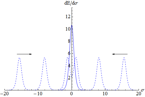
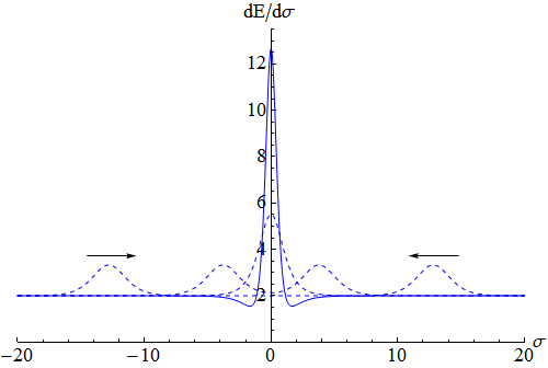
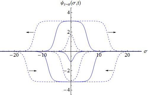
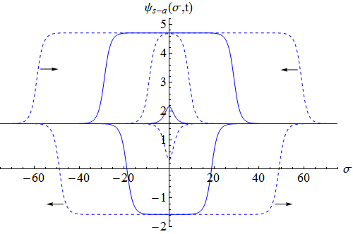
In figures 10 and 11 we have plotted the sG wavefunctions and energy densities for the kink-antikink scattering solutions that correspond to giant magnons (left) and single spikes (right) for $v=0.5$ and $\omega=2$. In a similar fashion we may obtain the solutions of the sG equation that correspond to soliton-soliton and antisoliton-antisoliton ($Q=\pm 2$) scattering between single spikes.
To obtain the phase-shift for single spikes, we may repeat the analysis of Hofman and Maldacena for the $\tau\leftrightarrow\sigma$ transformed solution (D.1). The result is the same if the soliton-soliton or the antisoliton-antisoliton solutions are used instead. In a reference frame where the soliton has velocity $v_{1}$ and the antisoliton has velocity $v_{2}$, the corresponding time delay is found to be:

ΔT121γ1logvcm,  vcm= tanh[θ^1θ^22](D.9)subscriptΔT121subscriptγ1subscriptlogvcmsubscript,  vcm= tanhdelimited-[]subscript^θ1subscript^θ22(D.9)\halign to=0.0pt{\relax\global\advance\@IEEEeqncolcnt by 1\relax\begingroup\csname @IEEEeqnarraycolPREc\endcsname#\relax\relax\relax\relax\relax\relax\relax\relax\relax\relax\csname @IEEEeqnarraycolPOSTc\endcsname\relax\relax\relax\relax\relax\relax\relax\relax\relax\relax\endgroup&\global\advance\@IEEEeqncolcnt by 1\relax\bgroup#\egroup&\global\advance\@IEEEeqncolcnt by 1\relax\hbox to\z@\bgroup\hss#\egroup\cr\hfil$\displaystyle\Delta T_{12} = \frac{1}{\gamma_{1}} \log v_{\text{cm}}\,, \quad v_{\text{cm}} = \tanh\left[\frac{\hat{\theta}_{1} - \hat{\theta}_{2}}{2}\right], $\hfil&{\vrule width=0.0pt,height=0.0pt,depth=0.0pt}&0.0pt{\hss{\normalcolor(D.9)}}\cr}

where $\cosh\hat{\theta}_{i}\equiv\gamma_{i}=(1-v_{i}^{2})^{-1/2}=\csc q_{i}/2$ for $i=1,2$. Just as for giant magnons, this quantity is negative in the center of mass frame, which means that the force between the two solitons is attractive. We find:

ΔT12= sinq12⋅log[1 - cosq1- q221 - cosq1+ q22](D.10)subscriptΔT12= sinsubscriptq12⋅logdelimited-[]1 - cossubscriptq1subscript- q221 - cossubscriptq1subscript+ q22(D.10)\halign to=0.0pt{\relax\global\advance\@IEEEeqncolcnt by 1\relax\begingroup\csname @IEEEeqnarraycolPREc\endcsname#\relax\relax\relax\relax\relax\relax\relax\relax\relax\relax\csname @IEEEeqnarraycolPOSTc\endcsname\relax\relax\relax\relax\relax\relax\relax\relax\relax\relax\endgroup&\global\advance\@IEEEeqncolcnt by 1\relax\bgroup#\egroup&\global\advance\@IEEEeqncolcnt by 1\relax\hbox to\z@\bgroup\hss#\egroup\cr\hfil$\displaystyle\Delta T_{12} = \sin\frac{q_{1}}{2}\cdot\log\left[\frac{1 - \cos\frac{q_{1} - q_{2}}{2}}{1 - \cos\frac{q_{1} + q_{2}}{2}}\right], $\hfil&{\vrule width=0.0pt,height=0.0pt,depth=0.0pt}&0.0pt{\hss{\normalcolor(D.10)}}\cr}

from which one may recover (D.1) by means of the formula,

ΔT12δ12ε1εiEipi2= arcsinJiqi2,  i = 1,2. (D.11)subscriptΔT12subscriptδ12subscriptε1subscriptεisubscriptEisubscriptpi2subscript= arcsinJisubscriptqi2,  i = 1,2. (D.11)\halign to=0.0pt{\relax\global\advance\@IEEEeqncolcnt by 1\relax\begingroup\csname @IEEEeqnarraycolPREc\endcsname#\relax\relax\relax\relax\relax\relax\relax\relax\relax\relax\csname @IEEEeqnarraycolPOSTc\endcsname\relax\relax\relax\relax\relax\relax\relax\relax\relax\relax\endgroup&\global\advance\@IEEEeqncolcnt by 1\relax\bgroup#\egroup&\global\advance\@IEEEeqncolcnt by 1\relax\hbox to\z@\bgroup\hss#\egroup\cr\hfil$\displaystyle\Delta T_{12} = \frac{\partial\delta_{12}}{\partial\varepsilon_{1}}\,,\quad\varepsilon_{i} \equiv\mathcal{E}_{i} - \frac{p_{i}}{2} = \arcsin\mathcal{J}_{i} = \frac{q_{i}}{2}\,, \quad i = 1,2. $\hfil&{\vrule width=0.0pt,height=0.0pt,depth=0.0pt}&0.0pt{\hss{\normalcolor(D.11)}}\cr}

These results are valid for $\sin q_{i}/2>0$.

Refer to caption
Refer to caption
Figure 12: sG wavefunction and energy density for breather-like solutions of single spikes.

D.2 Bound States

One may similarly $\tau\leftrightarrow\sigma$ transform any of the N-soliton solutions of the sG equation and obtain new (possibly unstable) solutions. For example the breather (Q = 0) solution,

tanψb2sina γaτa coshγaσγa11 + a2(D.12)tansubscriptψb2subscriptsina γaτsubscripta coshγaσsubscriptγa1superscript1 + a2(D.12)\halign to=0.0pt{\relax\global\advance\@IEEEeqncolcnt by 1\relax\begingroup\csname @IEEEeqnarraycolPREc\endcsname#\relax\relax\relax\relax\relax\relax\relax\relax\relax\relax\csname @IEEEeqnarraycolPOSTc\endcsname\relax\relax\relax\relax\relax\relax\relax\relax\relax\relax\endgroup&\global\advance\@IEEEeqncolcnt by 1\relax\bgroup#\egroup&\global\advance\@IEEEeqncolcnt by 1\relax\hbox to\z@\bgroup\hss#\egroup\cr\hfil$\displaystyle\tan\frac{\psi_{b}}{2} = \frac{\sin a \gamma_{a} \tau}{a\,\cosh\gamma_{a} \sigma}\,, \quad\gamma_{a} \equiv\frac{1}{\sqrt{1 + a^{2}}} $\hfil&{\vrule width=0.0pt,height=0.0pt,depth=0.0pt}&0.0pt{\hss{\normalcolor(D.12)}}\cr}

becomes under the $\tau\leftrightarrow\sigma$ transform:

tanψb2coshωγωτωsinγωσcoshωγωτωsinγωσ(D.13)tansubscriptψb2subscriptcoshωγωsubscriptτωsinγωσsubscriptcoshωγωsubscriptτωsinγωσ(D.13)\halign to=0.0pt{\relax\global\advance\@IEEEeqncolcnt by 1\relax\begingroup\csname @IEEEeqnarraycolPREc\endcsname#\relax\relax\relax\relax\relax\relax\relax\relax\relax\relax\csname @IEEEeqnarraycolPOSTc\endcsname\relax\relax\relax\relax\relax\relax\relax\relax\relax\relax\endgroup&\global\advance\@IEEEeqncolcnt by 1\relax\bgroup#\egroup&\global\advance\@IEEEeqncolcnt by 1\relax\hbox to\z@\bgroup\hss#\egroup\cr\hfil$\displaystyle\tan\frac{\psi_{b}}{2} = \frac{\cosh\omega\gamma_{\omega}\tau- \omega\sin\gamma_{\omega}\sigma}{\cosh\omega\gamma_{\omega}\tau+ \omega\sin\gamma_{\omega}\sigma}, $\hfil&{\vrule width=0.0pt,height=0.0pt,depth=0.0pt}&0.0pt{\hss{\normalcolor(D.13)}}\cr}

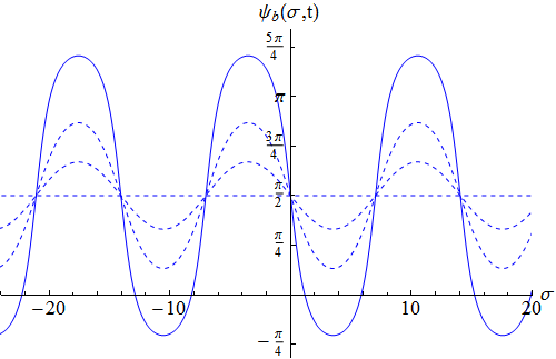
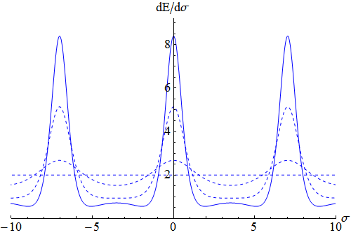
which again satisfies the sine-Gordon equation. In figure 12, we have plotted the wavefunction (left) and the energy density (right) of this sG solution for $\omega=2$. The solution is initially constant at $\psi=\pi/2$, then between times $\tau=-\tau_{0}$ and $\tau=0$ its amplitude and energy gradually grow until they become the wiggly periodic curves of figure 12 with extrema at $\sigma=k\pi/2\gamma_{\omega}$. After that, both curves start decreasing again towards the constant initial value of $\psi=\pi/2$ at $\tau=\tau_{0}$.
A stable 3-soliton solution of sG, comprised by a breather and a kink (or antikink), is known as the ”wobble” [58, 59]:

tanψw21 - a2asinaτeσ2(e-1 - a2σ+ ra2e1 - a2σ)cosh(1 - a2σ)1 - a2araeσsinaτ,  ra1 - 1 - a21 + 1 - a2(D.14)tansubscriptψw2superscript1 - a2asinaτsuperscripteσ2superscripte-superscript1 - a2σsuperscriptsubscript+ ra2superscriptesuperscript1 - a2σcoshsuperscript1 - a2σsuperscript1 - a2asubscriptrasuperscripteσsinaτsubscript,  ra1 - superscript1 - a21 + superscript1 - a2(D.14)\halign to=0.0pt{\relax\global\advance\@IEEEeqncolcnt by 1\relax\begingroup\csname @IEEEeqnarraycolPREc\endcsname#\relax\relax\relax\relax\relax\relax\relax\relax\relax\relax\csname @IEEEeqnarraycolPOSTc\endcsname\relax\relax\relax\relax\relax\relax\relax\relax\relax\relax\endgroup&\global\advance\@IEEEeqncolcnt by 1\relax\bgroup#\egroup&\global\advance\@IEEEeqncolcnt by 1\relax\hbox to\z@\bgroup\hss#\egroup\cr\hfil$\displaystyle\tan\frac{\psi_{w}}{2} = \frac{\frac{\sqrt{1 - a^{2}}}{a}\sin a\tau+ \frac{e^{\sigma}}{2} \left(e^{-\sqrt{1 - a^{2}}\sigma} + r_{\text{a}}^{2} e^{\sqrt{1 - a^{2}}\sigma}\right)}{\cosh\left(\sqrt{1 - a^{2}}\,\sigma\right) + \frac{\sqrt{1 - a^{2}}}{a} \, r_{\text{a}} \, e^{\sigma}\sin a\tau}\,, \quad r_{\text{a}} \equiv\frac{1 - \sqrt{1 - a^{2}}}{1 + \sqrt{1 - a^{2}}}. $\hfil&{\vrule width=0.0pt,height=0.0pt,depth=0.0pt}&0.0pt{\hss{\normalcolor(D.14)}}\cr}

Under the $\tau\leftrightarrow\sigma$ transform it becomes:

tanψw2ω2- 1(rωeτ- 1)sinσω12[(1 - eτ)e-ω2- 1ωτ(1 - rω2eτ)eω2- 1ωτ]ω2- 1(rωeτ+ 1)sinσω12[(1 + eτ)e-ω2- 1ωτ(1 + rω2eτ)eω2- 1ωτ](D.15)tansubscriptψw2superscriptω2- 1subscriptrωsuperscripteτ- 1sinσω12delimited-[]superscript1 - eτsuperscripte-superscriptω2- 1ωτsuperscriptsubscript1 - rω2superscripteτsuperscriptesuperscriptω2- 1ωτsuperscriptω2- 1subscriptrωsuperscripteτ+ 1sinσω12delimited-[]superscript1 + eτsuperscripte-superscriptω2- 1ωτsuperscriptsubscript1 + rω2superscripteτsuperscriptesuperscriptω2- 1ωτ(D.15)\halign to=0.0pt{\relax\global\advance\@IEEEeqncolcnt by 1\relax\begingroup\csname @IEEEeqnarraycolPREc\endcsname#\relax\relax\relax\relax\relax\relax\relax\relax\relax\relax\csname @IEEEeqnarraycolPOSTc\endcsname\relax\relax\relax\relax\relax\relax\relax\relax\relax\relax\endgroup&\global\advance\@IEEEeqncolcnt by 1\relax\bgroup#\egroup&\global\advance\@IEEEeqncolcnt by 1\relax\hbox to\z@\bgroup\hss#\egroup\cr\hfil$\displaystyle\tan\frac{\psi_{w}}{2} = \frac{\sqrt{\omega^{2} - 1}\left(r_{\omega} e^{\tau}- 1\right) \sin\frac{\sigma}{\omega} + \frac{1}{2}\left[\left(1 - e^{\tau}\right)e^{-\frac{\sqrt{\omega^{2} - 1}}{\omega}\cdot\tau} + \left(1 - r_{\omega}^{2} \, e^{\tau}\right)e^{\frac{\sqrt{\omega^{2} - 1}}{\omega}\cdot\tau}\right]}{\sqrt{\omega^{2} - 1}\left(r_{\omega} e^{\tau}+ 1\right) \sin\frac{\sigma}{\omega} + \frac{1}{2}\left[\left(1 + e^{\tau}\right)e^{-\frac{\sqrt{\omega^{2} - 1}}{\omega}\cdot\tau} + \left(1 + r_{\omega}^{2} \, e^{\tau}\right)e^{\frac{\sqrt{\omega^{2} - 1}}{\omega}\cdot\tau}\right]}, $\hfil&{\vrule width=0.0pt,height=0.0pt,depth=0.0pt}&0.0pt{\hss{\normalcolor(D.15)}}\cr}

where

rωωω2- 1ωω2- 1(D.16)subscriptrωωsuperscriptω2- 1ωsuperscriptω2- 1(D.16)\halign to=0.0pt{\relax\global\advance\@IEEEeqncolcnt by 1\relax\begingroup\csname @IEEEeqnarraycolPREc\endcsname#\relax\relax\relax\relax\relax\relax\relax\relax\relax\relax\csname @IEEEeqnarraycolPOSTc\endcsname\relax\relax\relax\relax\relax\relax\relax\relax\relax\relax\endgroup&\global\advance\@IEEEeqncolcnt by 1\relax\bgroup#\egroup&\global\advance\@IEEEeqncolcnt by 1\relax\hbox to\z@\bgroup\hss#\egroup\cr\hfil$\displaystyle r_{\omega}\equiv\frac{\omega- \sqrt{\omega^{2} - 1}}{\omega+ \sqrt{\omega^{2} - 1}}. $\hfil&{\vrule width=0.0pt,height=0.0pt,depth=0.0pt}&0.0pt{\hss{\normalcolor(D.16)}}\cr}

This solution also exhibits the ”flare”-like behavior of the breather that we saw above.

Appendix E Lambert’s W-Function

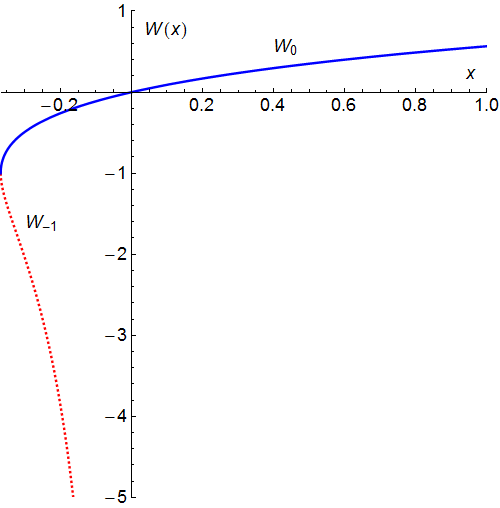
Since our paper relies essentially on the Lambert W-function, we shall review here some of its basic properties. The Lambert W-function is defined implicitly by the following relation:

W(z)eW(z)= z ⇔W(z ez)= z. (E.1)WzsuperscripteWz= z ⇔Wsuperscriptz ez= z. (E.1)\halign to=0.0pt{\relax\global\advance\@IEEEeqncolcnt by 1\relax\begingroup\csname @IEEEeqnarraycolPREc\endcsname#\relax\relax\relax\relax\relax\relax\relax\relax\relax\relax\csname @IEEEeqnarraycolPOSTc\endcsname\relax\relax\relax\relax\relax\relax\relax\relax\relax\relax\endgroup&\global\advance\@IEEEeqncolcnt by 1\relax\bgroup#\egroup&\global\advance\@IEEEeqncolcnt by 1\relax\hbox to\z@\bgroup\hss#\egroup\cr\hfil$\displaystyle W\left(z\right)\,e^{W\left(z\right)} = z \Leftrightarrow W\left(z\,e^{z}\right) = z. $\hfil&{\vrule width=0.0pt,height=0.0pt,depth=0.0pt}&0.0pt{\hss{\normalcolor(E.1)}}\cr}

It has two real branches, $W_{0}\left(x\right)$ for $x\in\left[-e^{-1},\infty\right)$ and $W_{-1}\left(x\right)$ for $x\in\left[-e^{-1},0\right]$ that have been plotted in figure 13. The branch point is $W\left(-e^{-1}\right)=-1$. The Taylor series around $x=0$ for each of the two branches are [60]:

W0(x)= ∑n = 0(-1)n(n+1)n(n+1)!⋅xn+1= ∑n = 1(-1)n + 1nn - 1n!⋅xn,  —x— ≤e-1(E.2)W-1(x)= ln—x— - ln—ln—x—— + ∑n = 0m = 1(-1)nm![n + m n + 1](ln—x—)-n-m(ln—ln—x——)m(E.3)subscriptW0xsuperscriptsubscript= ∑n = 0superscript-1nsuperscriptn+1nn+1!superscript⋅xn+1superscriptsubscript= ∑n = 1superscript-1n + 1superscriptnn - 1n!superscript⋅xnsuperscript,  —x— ≤e-1(E.2)missing-subexpressionsubscriptW-1xsuperscriptsubscript= ln—x— - ln—ln—x—— + ∑n = 0superscriptsubscriptm = 1superscript-1nm!FRACOPn + m n + 1superscriptln—x—-n-msuperscriptln—ln—x——m(E.3)\halign to=0.0pt{\relax\global\advance\@IEEEeqncolcnt by 1\relax\begingroup\csname @IEEEeqnarraycolPREl\endcsname#\relax\relax\relax\relax\relax\relax\relax\relax\relax\relax\csname @IEEEeqnarraycolPOSTl\endcsname\relax\relax\relax\relax\relax\relax\relax\relax\relax\relax\endgroup&\global\advance\@IEEEeqncolcnt by 1\relax\bgroup#\egroup&\global\advance\@IEEEeqncolcnt by 1\relax\hbox to\z@\bgroup\hss#\egroup\cr$\displaystyle W_{0}\left(x\right) = \sum_{n = 0}^{\infty}\left(-1\right)^{n}\frac{\left(n+1\right)^{n}}{\left(n+1\right)!}\cdot x^{n+1} = \sum_{n = 1}^{\infty}\left(-1\right)^{n + 1} \frac{n^{n - 1}}{n!}\cdot x^{n}\,, \quad\left|x\right| \leq e^{-1} $\hfil&{{}\vrule width=0.0pt,height=0.0pt,depth=0.0pt}&0.0pt{\hss{\normalcolor(E.2)}}\cr\penalty 0\vskip 3.0pt\vskip 12.0pt\cr$\displaystyle W_{-1}\left(x\right) = \ln\left|x\right| - \ln\left|\ln\left|x\right|\right| + \sum_{n = 0}^{\infty}\sum_{m = 1}^{\infty}\frac{\left(-1\right)^{n}}{m!} {n + m \brack n + 1} \left(\ln\left|x\right|\right)^{-n-m} \left(\ln\left|\ln\left|x\right|\right|\right)^{m}, \qquad $\hfil&{\vrule width=0.0pt,height=0.0pt,depth=0.0pt}&0.0pt{\hss{\normalcolor(E.3)}}\cr}

where the unsigned Stirling numbers of the first kind, $\left[\begin{array}[]{c}n+m\\ n+1\end{array}\right]$ are defined recursively from [61]:

[nk][n - 1k - 1](n - 1)[n - 1k][n0][0k]= 0 , [00]= 1 ,  n,k≥1. (E.4)delimited-[]nkdelimited-[]n - 1k - 1n - 1delimited-[]n - 1kdelimited-[]n0delimited-[]0k= 0 , delimited-[]00= 1 ,  n,k≥1. (E.4)\halign to=0.0pt{\relax\global\advance\@IEEEeqncolcnt by 1\relax\begingroup\csname @IEEEeqnarraycolPREc\endcsname#\relax\relax\relax\relax\relax\relax\relax\relax\relax\relax\csname @IEEEeqnarraycolPOSTc\endcsname\relax\relax\relax\relax\relax\relax\relax\relax\relax\relax\endgroup&\global\advance\@IEEEeqncolcnt by 1\relax\bgroup#\egroup&\global\advance\@IEEEeqncolcnt by 1\relax\hbox to\z@\bgroup\hss#\egroup\cr\hfil$\displaystyle\left[\begin{array}[]{c}n\\ k\end{array}\right] = \left[\begin{array}[]{c}n - 1\\ k - 1\end{array}\right] + \left(n - 1\right)\left[\begin{array}[]{c}n - 1\\ k\end{array}\right] \quad\& \quad\left[\begin{array}[]{c}n\\ 0\end{array}\right] = \left[\begin{array}[]{c}0\\ k\end{array}\right] = 0\,, \ \left[\begin{array}[]{c}0\\ 0\end{array}\right] = 1\,, \quad n,k\geq 1. \qquad $\hfil&{\vrule width=0.0pt,height=0.0pt,depth=0.0pt}&0.0pt{\hss{\normalcolor(E.4)}}\cr}
Refer to caption
Figure 13: Lambert’s W-function.

Using the defining property (E), we may obtain simplified expressions for the derivatives and antiderivatives of Lambert’s W-function. Here are some useful expressions that we employ in our paper:

W’(x)W(x)x(1 + W(x))(E.5)x W’(x)= ∑n = 1(-1)n + 1nnn!⋅xnW(x)1 + W(x)(E.6)(x W’(x))’ = ∑n = 1(-1)n + 1nn + 1n!⋅xnW(x)(1 + W(x))3(E.7)∫W(x)dx = x(W(x)- 1 + 1W(x))(E.8)W(x)xdx = ∑n = 1(-1)n + 1nn - 2n!⋅xn= W(x)W2(x)2(E.9)1xW(x)xdx2= ∑n = 1(-1)n + 1nn - 3n!⋅xn= W(x)3W2(x)4W3(x)6(E.10)W’xWxx1 + Wx(E.5)missing-subexpressionx W’xsuperscriptsubscript= ∑n = 1superscript-1n + 1superscriptnnn!superscript⋅xnWx1 + Wx(E.6)missing-subexpressionx W’xsuperscriptsubscript’ = ∑n = 1superscript-1n + 1superscriptnn + 1n!superscript⋅xnWxsuperscript1 + Wx3(E.7)missing-subexpression∫Wxdx = xWx- 1 + 1Wx(E.8)missing-subexpressionWxxsuperscriptsubscriptdx = ∑n = 1superscript-1n + 1superscriptnn - 2n!superscript⋅xn= WxsuperscriptW2x2(E.9)missing-subexpression1xWxxsuperscriptdx2superscriptsubscript= ∑n = 1superscript-1n + 1superscriptnn - 3n!superscript⋅xn= Wxsuperscript3W2x4superscriptW3x6(E.10)\halign to=0.0pt{\relax\global\advance\@IEEEeqncolcnt by 1\relax\begingroup\csname @IEEEeqnarraycolPREc\endcsname#\relax\relax\relax\relax\relax\relax\relax\relax\relax\relax\csname @IEEEeqnarraycolPOSTc\endcsname\relax\relax\relax\relax\relax\relax\relax\relax\relax\relax\endgroup&\global\advance\@IEEEeqncolcnt by 1\relax\bgroup#\egroup&\global\advance\@IEEEeqncolcnt by 1\relax\hbox to\z@\bgroup\hss#\egroup\cr\hfil$\displaystyle W'\left(x\right) = \frac{W\left(x\right)}{x\left(1 + W\left(x\right)\right)} $\hfil&{{}\vrule width=0.0pt,height=0.0pt,depth=0.0pt}&0.0pt{\hss{\normalcolor(E.5)}}\cr\penalty 0\vskip 3.0pt\vskip 12.0pt\cr\hfil$\displaystyle x\,W'\left(x\right) = \sum_{n = 1}^{\infty}\left(-1\right)^{n + 1} \frac{n^{n}}{n!}\cdot x^{n} = \frac{W\left(x\right)}{1 + W\left(x\right)} $\hfil&{{}\vrule width=0.0pt,height=0.0pt,depth=0.0pt}&0.0pt{\hss{\normalcolor(E.6)}}\cr\penalty 0\vskip 3.0pt\vskip 12.0pt\cr\hfil$\displaystyle x\,\left(x\,W'\left(x\right)\right)' = \sum_{n = 1}^{\infty}\left(-1\right)^{n + 1} \frac{n^{n + 1}}{n!}\cdot x^{n} = \frac{W\left(x\right)}{\left(1 + W\left(x\right)\right)^{3}} $\hfil&{{}\vrule width=0.0pt,height=0.0pt,depth=0.0pt}&0.0pt{\hss{\normalcolor(E.7)}}\cr\penalty 0\vskip 3.0pt\vskip 12.0pt\cr\hfil$\displaystyle\int W\left(x\right) \ dx = x\left(W\left(x\right) - 1 + \frac{1}{W\left(x\right)}\right) $\hfil&{{}\vrule width=0.0pt,height=0.0pt,depth=0.0pt}&0.0pt{\hss{\normalcolor(E.8)}}\cr\penalty 0\vskip 3.0pt\vskip 12.0pt\cr\hfil$\displaystyle\int\frac{W\left(x\right)}{x} \ dx = \sum_{n = 1}^{\infty}\left(-1\right)^{n + 1} \frac{n^{n - 2}}{n!}\cdot x^{n} = W\left(x\right) + \frac{W^{2}\left(x\right)}{2} $\hfil&{{}\vrule width=0.0pt,height=0.0pt,depth=0.0pt}&0.0pt{\hss{\normalcolor(E.9)}}\cr\penalty 0\vskip 3.0pt\vskip 12.0pt\cr\hfil$\displaystyle\int\frac{1}{x} \int\frac{W\left(x\right)}{x} \ dx^{2} = \sum_{n = 1}^{\infty}\left(-1\right)^{n + 1} \frac{n^{n - 3}}{n!}\cdot x^{n} = W\left(x\right) + \frac{3W^{2}\left(x\right)}{4} + \frac{W^{3}\left(x\right)}{6}. \qquad $\hfil&{\vrule width=0.0pt,height=0.0pt,depth=0.0pt}&0.0pt{\hss{\normalcolor(E.10)}}\cr}

Appendix F Elliptic Integrals and Jacobian Elliptic Functions

This appendix contains the definitions and some basic properties of elliptic integrals and Jacobian elliptic functions that we use in our paper. Our conventions mainly follow Abramowitz-Stegun [62].
Jacobian Elliptic Functions

u ≡∫0φdθ(1 - m sin2θ)1/2φ≡am(u — m)  ,  Δ(φ) ≡(1 - sin2θ)1/2≡dn(u — m) (F.1)&x=sinφsn(u|m),cosφcn(u|m).(F.2) formulae-sequencesuperscriptsubscriptu ≡∫0φdθsuperscriptsuperscript1 - m sin2θ1/2superscriptφ≡am(u — m)  ,  Δ(φ) ≡(1 - sin2superscriptθ)1/2≡dn(u — m) (F.1)&𝑥𝜑𝑠𝑛conditional𝑢𝑚𝜑𝑐𝑛conditional𝑢𝑚F.2 \halign to=0.0pt{\relax\global\advance\@IEEEeqncolcnt by 1\relax\begingroup\csname @IEEEeqnarraycolPREl\endcsname#\relax\relax\relax\relax\relax\relax\relax\relax\relax\relax\csname @IEEEeqnarraycolPOSTl\endcsname\relax\relax\relax\relax\relax\relax\relax\relax\relax\relax\endgroup&\relax\global\advance\@IEEEeqncolcnt by 1\relax\begingroup\csname @IEEEeqnarraycolPREl\endcsname#\relax\relax\relax\relax\relax\relax\relax\relax\relax\relax\csname @IEEEeqnarraycolPOSTl\endcsname\relax\relax\relax\relax\relax\relax\relax\relax\relax\relax\endgroup&\global\advance\@IEEEeqncolcnt by 1\relax\bgroup#\egroup&\global\advance\@IEEEeqncolcnt by 1\relax\hbox to\z@\bgroup\hss#\egroup\cr$\displaystyle u \equiv\int_{0}^{\varphi}\frac{d\theta}{\left(1 - m \sin^{2}\theta\right)^{1/2}} \,, \quad$\hfil&$\displaystyle\varphi\equiv am(u | m) \,, \quad\Delta(\varphi) \equiv(1 - \sin^{2}\theta)^{1/2} \equiv dn(u | m) $\hfil&{{}\vrule width=0.0pt,height=0.0pt,depth=0.0pt&0.0pt{\hss{\normalcolor(F.1)}}\cr\penalty 0\vskip 3.0pt\vskip 0.0pt\cr}&x=\sin\varphi\equiv sn(u|m)\,,\quad\cos\varphi\equiv cn(u|m).\vrule width=0.0pt,height=0.0pt,depth=0.0pt{\normalcolor(F.2)}\cr}

Elliptic Integral of the First Kind

F(φ m)≡∫0φ(1 - m sin2θ)-1/2dθ= ∫0x[(1 - t2)(1 - m t2)]-1/2dt = u (F.3)K(m)F(π2 m)π2F12[12,12;1;m](complete) (F.4)Fφ msuperscriptsubscript≡∫0φsuperscriptsuperscript1 - m sin2θ-1/2superscriptsubscriptdθ= ∫0xsuperscriptdelimited-[]superscript1 - t2superscript1 - m t2-1/2dt = u (F.3)missing-subexpressionKmFπ2 mπ2subscriptsubscriptF12delimited-[]12,12;1;m(complete) (F.4)\halign to=0.0pt{\relax\global\advance\@IEEEeqncolcnt by 1\relax\begingroup\csname @IEEEeqnarraycolPREl\endcsname#\relax\relax\relax\relax\relax\relax\relax\relax\relax\relax\csname @IEEEeqnarraycolPOSTl\endcsname\relax\relax\relax\relax\relax\relax\relax\relax\relax\relax\endgroup&\global\advance\@IEEEeqncolcnt by 1\relax\bgroup#\egroup&\global\advance\@IEEEeqncolcnt by 1\relax\hbox to\z@\bgroup\hss#\egroup\cr$\displaystyle\mathbb{F}\left(\varphi\big{|} m\right) \equiv\int_{0}^{\varphi}\left(1 - m\,\sin^{2}\theta\right)^{-1/2} \, d\theta= \int_{0}^{x} \left[\left(1 - t^{2}\right)\left(1 - m\,t^{2}\right)\right]^{-1/2} \, dt = u \qquad $\hfil&{{}\vrule width=0.0pt,height=0.0pt,depth=0.0pt}&0.0pt{\hss{\normalcolor(F.3)}}\cr\penalty 0\vskip 3.0pt\vskip 12.0pt\cr$\displaystyle\mathbb{K}\left(m\right) \equiv\mathbb{F}\left(\frac{\pi}{2} \Big{|} m\right) = \frac{\pi}{2} \cdot{{}_{2}\mathcal{F}_{1}}\left[\frac{1}{2},\frac{1}{2};1;m\right] \quad\text{(complete)} $\hfil&{\vrule width=0.0pt,height=0.0pt,depth=0.0pt}&0.0pt{\hss{\normalcolor(F.4)}}\cr}
K(m)π2⋅∑n = 0((2n - 1)!!(2n)!!)2mn(F.5) = π2[1 + (12)2m + (1 ⋅32 ⋅4)2m2(1 ⋅3 ⋅52 ⋅4 ⋅6)2m3+ …],  —m— ¡ 1 (F.6)Kmπ2superscriptsubscript⋅∑n = 0superscript(2n - 1)!!(2n)!!2superscriptmn(F.5)missing-subexpression = π2delimited-[]1 + superscript122m + superscript1 ⋅32 ⋅42superscriptm2superscript1 ⋅3 ⋅52 ⋅4 ⋅62superscriptm3+ …,  —m— ¡ 1 (F.6)\halign to=0.0pt{\relax\global\advance\@IEEEeqncolcnt by 1\relax\begingroup\csname @IEEEeqnarraycolPREl\endcsname#\relax\relax\relax\relax\relax\relax\relax\relax\relax\relax\csname @IEEEeqnarraycolPOSTl\endcsname\relax\relax\relax\relax\relax\relax\relax\relax\relax\relax\endgroup&\relax\global\advance\@IEEEeqncolcnt by 1\relax\begingroup\csname @IEEEeqnarraycolPREl\endcsname#\relax\relax\relax\relax\relax\relax\relax\relax\relax\relax\csname @IEEEeqnarraycolPOSTl\endcsname\relax\relax\relax\relax\relax\relax\relax\relax\relax\relax\endgroup&\global\advance\@IEEEeqncolcnt by 1\relax\bgroup#\egroup&\global\advance\@IEEEeqncolcnt by 1\relax\hbox to\z@\bgroup\hss#\egroup\cr$\displaystyle\mathbb{K}\left(m\right) = \frac{\pi}{2} \cdot\sum_{n = 0}^{\infty}$\hfil&$\displaystyle\left(\frac{(2n - 1)!!}{(2n)!!}\right)^{2} m^{n} = $\hfil&{{}\vrule width=0.0pt,height=0.0pt,depth=0.0pt}&0.0pt{\hss{\normalcolor(F.5)}}\cr\penalty 0\vskip 3.0pt\vskip 12.0pt\cr$\displaystyle$\hfil&$\displaystyle\qquad= \frac{\pi}{2}\cdot\left[1 + \left(\frac{1}{2}\right)^{2} m + \left(\frac{1 \cdot 3}{2 \cdot 4}\right)^{2} m^{2} + \left(\frac{1 \cdot 3 \cdot 5}{2 \cdot 4 \cdot 6}\right)^{2} m^{3} + \ldots\right] \,, \quad|m| < 1 \qquad$\hfil&{\vrule width=0.0pt,height=0.0pt,depth=0.0pt}&0.0pt{\hss{\normalcolor(F.6)}}\cr}
K(m)1π⋅∑n = 0(Γ(n + 1/2)n!)2[2ψ(n + 1)- 2ψ(n + 1/2)- ln(1 - m)](1 - m)n(F.7)= ∑n = 0((2n - 1)!!(2n)!!)2[ψ(n + 1)ψ(n + 1/2)12ln(1 - m)](1 - m)n,  —1 - m— ¡ 1, (F.8)Km1πsuperscriptsubscript⋅∑n = 0superscriptΓn + 1/2n!2delimited-[]2ψn + 1- 2ψn + 1/2- ln1 - msuperscript1 - mn(F.7)missing-subexpressionsuperscriptsubscript= ∑n = 0superscript2n - 1!!2n!!2delimited-[]ψn + 1ψn + 1/212ln1 - msuperscript1 - mn,  —1 - m— ¡ 1, (F.8)\halign to=0.0pt{\relax\global\advance\@IEEEeqncolcnt by 1\relax\begingroup\csname @IEEEeqnarraycolPREl\endcsname#\relax\relax\relax\relax\relax\relax\relax\relax\relax\relax\csname @IEEEeqnarraycolPOSTl\endcsname\relax\relax\relax\relax\relax\relax\relax\relax\relax\relax\endgroup&\relax\global\advance\@IEEEeqncolcnt by 1\relax\begingroup\csname @IEEEeqnarraycolPREl\endcsname#\relax\relax\relax\relax\relax\relax\relax\relax\relax\relax\csname @IEEEeqnarraycolPOSTl\endcsname\relax\relax\relax\relax\relax\relax\relax\relax\relax\relax\endgroup&\global\advance\@IEEEeqncolcnt by 1\relax\bgroup#\egroup&\global\advance\@IEEEeqncolcnt by 1\relax\hbox to\z@\bgroup\hss#\egroup\cr$\displaystyle\mathbb{K}\left(m\right) $\hfil&$\displaystyle= \frac{1}{2 \pi} \cdot\sum_{n = 0}^{\infty}\left(\frac{\Gamma\left(n + 1/2\right)}{n!}\right)^{2} \left[2\psi\left(n + 1\right) - 2\psi\left(n + 1/2\right) - \ln\left(1 - m\right)\right] \, \left(1 - m\right)^{n} = $\hfil&{{}\vrule width=0.0pt,height=0.0pt,depth=0.0pt}&0.0pt{\hss{\normalcolor(F.7)}}\cr\penalty 0\vskip 3.0pt\vskip 12.0pt\cr$\displaystyle$\hfil&$\displaystyle= \sum_{n = 0}^{\infty}\left(\frac{\left(2n - 1\right)!!}{\left(2n\right)!!}\right)^{2} \left[\psi\left(n + 1\right) - \psi\left(n + 1/2\right) - \frac{1}{2}\ln\left(1 - m\right)\right] \, \left(1 - m\right)^{n} \,, \quad\left|1 - m\right| < 1, \qquad$\hfil&{\vrule width=0.0pt,height=0.0pt,depth=0.0pt}&0.0pt{\hss{\normalcolor(F.8)}}\cr}

where $\psi(z)\equiv\Gamma^{\prime}(z)/\Gamma(z)$ is the psi/digamma function.
Elliptic Integral of the Second Kind

E(φ m)≡∫0φ(1 - m sin2θ)1/2dθ= ∫0x(1 - t2)-1/2(1 - m t2)1/2dt (F.9)E(m)E(π2 m)π2F12[-12,12;1;m](complete) (F.10)Eφ msuperscriptsubscript≡∫0φsuperscriptsuperscript1 - m sin2θ1/2superscriptsubscriptdθ= ∫0xsuperscriptsuperscript1 - t2-1/2superscriptsuperscript1 - m t21/2dt (F.9)missing-subexpressionEmEπ2 mπ2subscriptsubscriptF12delimited-[]-12,12;1;m(complete) (F.10)\halign to=0.0pt{\relax\global\advance\@IEEEeqncolcnt by 1\relax\begingroup\csname @IEEEeqnarraycolPREl\endcsname#\relax\relax\relax\relax\relax\relax\relax\relax\relax\relax\csname @IEEEeqnarraycolPOSTl\endcsname\relax\relax\relax\relax\relax\relax\relax\relax\relax\relax\endgroup&\global\advance\@IEEEeqncolcnt by 1\relax\bgroup#\egroup&\global\advance\@IEEEeqncolcnt by 1\relax\hbox to\z@\bgroup\hss#\egroup\cr$\displaystyle\mathbb{E}\left(\varphi\big{|} m\right) \equiv\int_{0}^{\varphi}\left(1 - m\,\sin^{2}\theta\right)^{1/2} \, d\theta= \int_{0}^{x} \left(1 - t^{2}\right)^{-1/2} \left(1 - m\,t^{2}\right)^{1/2} \, dt \qquad $\hfil&{{}\vrule width=0.0pt,height=0.0pt,depth=0.0pt}&0.0pt{\hss{\normalcolor(F.9)}}\cr\penalty 0\vskip 3.0pt\vskip 12.0pt\cr$\displaystyle\mathbb{E}\left(m\right) \equiv\mathbb{E}\left(\frac{\pi}{2} \Big{|} m\right) = \frac{\pi}{2} \cdot{{}_{2}\mathcal{F}_{1}}\left[-\frac{1}{2},\frac{1}{2};1;m\right] \quad\text{(complete)} $\hfil&{\vrule width=0.0pt,height=0.0pt,depth=0.0pt}&0.0pt{\hss{\normalcolor(F.10)}}\cr}
E(m)= - π2⋅∑n = 0((2n - 1)!!(2n)!!)2mn2n - 1(F.11) = π2[1 - (12)2m1(1 ⋅32 ⋅4)2m23(1 ⋅3 ⋅52 ⋅4 ⋅6)2m35+ …],  —m— ¡ 1 (F.12)Em= - π2superscriptsubscript⋅∑n = 0superscript(2n - 1)!!(2n)!!2superscriptmn2n - 1(F.11)missing-subexpression = π2delimited-[]1 - superscript122m1superscript1 ⋅32 ⋅42superscriptm23superscript1 ⋅3 ⋅52 ⋅4 ⋅62superscriptm35+ …,  —m— ¡ 1 (F.12)\halign to=0.0pt{\relax\global\advance\@IEEEeqncolcnt by 1\relax\begingroup\csname @IEEEeqnarraycolPREl\endcsname#\relax\relax\relax\relax\relax\relax\relax\relax\relax\relax\csname @IEEEeqnarraycolPOSTl\endcsname\relax\relax\relax\relax\relax\relax\relax\relax\relax\relax\endgroup&\relax\global\advance\@IEEEeqncolcnt by 1\relax\begingroup\csname @IEEEeqnarraycolPREl\endcsname#\relax\relax\relax\relax\relax\relax\relax\relax\relax\relax\csname @IEEEeqnarraycolPOSTl\endcsname\relax\relax\relax\relax\relax\relax\relax\relax\relax\relax\endgroup&\global\advance\@IEEEeqncolcnt by 1\relax\bgroup#\egroup&\global\advance\@IEEEeqncolcnt by 1\relax\hbox to\z@\bgroup\hss#\egroup\cr$\displaystyle\mathbb{E}\left(m\right) = - \frac{\pi}{2} \cdot\sum_{n = 0}^{\infty}$\hfil&$\displaystyle\left(\frac{(2n - 1)!!}{(2n)!!}\right)^{2} \frac{m^{n}}{2n - 1} = $\hfil&{{}\vrule width=0.0pt,height=0.0pt,depth=0.0pt}&0.0pt{\hss{\normalcolor(F.11)}}\cr\penalty 0\vskip 3.0pt\vskip 12.0pt\cr$\displaystyle$\hfil&$\displaystyle\quad= \frac{\pi}{2} \cdot\left[1 - \left(\frac{1}{2}\right)^{2} \frac{m}{1} - \left(\frac{1 \cdot 3}{2 \cdot 4}\right)^{2} \frac{m^{2}}{3} - \left(\frac{1 \cdot 3 \cdot 5}{2 \cdot 4 \cdot 6}\right)^{2} \frac{m^{3}}{5} + \ldots\right] \,, \quad|m| < 1 \qquad$\hfil&{\vrule width=0.0pt,height=0.0pt,depth=0.0pt}&0.0pt{\hss{\normalcolor(F.12)}}\cr}
E(m)= 1 1π⋅∑n = 0Γ(n + 1/2)Γ(n + 3/2)n!(n + 1)![ln(1 - m)ψ(n + 1/2)ψ(n + 3/2)ψ(n + 1)(F.13)-ψ(n + 2)] (1 - m)n + 1(F.14)= 1 + ∑n = 1(2n - 1)[(2n - 3)!!]2(2n - 2)!!(2n)!![ψ(n)ψ(n - 1/2)12n(2n - 1)12ln(1 - m)] (1 - m)n(F.15)—1 - m— ¡ 1. (F.16)Em= 1 1πsuperscriptsubscript⋅∑n = 0Γn + 1/2Γn + 3/2n!n + 1![ln1 - mψn + 1/2ψn + 3/2ψn + 1(F.13)missing-subexpressionmissing-subexpression-ψn + 2] superscript1 - mn + 1(F.14)missing-subexpression= 1 superscriptsubscript+ ∑n = 12n - 1superscriptdelimited-[]2n - 3!!22n - 2!!2n!![ψnψn - 1/212n2n - 112ln1 - m] superscript1 - mn(F.15)missing-subexpressionmissing-subexpression—1 - m— ¡ 1. (F.16)\halign to=0.0pt{\relax\global\advance\@IEEEeqncolcnt by 1\relax\begingroup\csname @IEEEeqnarraycolPREl\endcsname#\relax\relax\relax\relax\relax\relax\relax\relax\relax\relax\csname @IEEEeqnarraycolPOSTl\endcsname\relax\relax\relax\relax\relax\relax\relax\relax\relax\relax\endgroup&\relax\global\advance\@IEEEeqncolcnt by 1\relax\begingroup\csname @IEEEeqnarraycolPREl\endcsname#\relax\relax\relax\relax\relax\relax\relax\relax\relax\relax\csname @IEEEeqnarraycolPOSTl\endcsname\relax\relax\relax\relax\relax\relax\relax\relax\relax\relax\endgroup&\relax\global\advance\@IEEEeqncolcnt by 1\relax\begingroup\csname @IEEEeqnarraycolPREl\endcsname#\relax\relax\relax\relax\relax\relax\relax\relax\relax\relax\csname @IEEEeqnarraycolPOSTl\endcsname\relax\relax\relax\relax\relax\relax\relax\relax\relax\relax\endgroup&\global\advance\@IEEEeqncolcnt by 1\relax\bgroup#\egroup&\global\advance\@IEEEeqncolcnt by 1\relax\hbox to\z@\bgroup\hss#\egroup\cr$\displaystyle\mathbb{E}\left(m\right) $\hfil&$\displaystyle= 1 $\hfil&$\displaystyle- \frac{1}{2 \pi} \cdot\sum_{n = 0}^{\infty}\frac{\Gamma\left(n + 1/2\right) \Gamma\left(n + 3/2\right)}{n!\left(n + 1\right)!} \bigg{[}\ln\left(1 - m\right) + \psi\left(n + 1/2\right) + \psi\left(n + 3/2\right) - \psi\left(n + 1\right) - $\hfil&{{}\vrule width=0.0pt,height=0.0pt,depth=0.0pt}&0.0pt{\hss{\normalcolor(F.13)}}\cr\penalty 0\vskip 3.0pt\vskip 12.0pt\cr$\displaystyle$\hfil&$\displaystyle$\hfil&$\displaystyle-\psi\left(n + 2\right)\bigg{]} \, \left(1 - m\right)^{n + 1} = $\hfil&{{}\vrule width=0.0pt,height=0.0pt,depth=0.0pt}&0.0pt{\hss{\normalcolor(F.14)}}\cr\penalty 0\vskip 3.0pt\vskip 12.0pt\cr$\displaystyle$\hfil&$\displaystyle= 1 $\hfil&$\displaystyle+ \sum_{n = 1}^{\infty}\frac{\left(2n - 1\right)\left[\left(2n - 3\right)!!\right]^{2}}{\left(2n - 2\right)!!\left(2n\right)!!} \bigg{[}\psi\left(n\right) - \psi\left(n - 1/2\right) - \frac{1}{2n\left(2n - 1\right)} - \frac{1}{2}\ln\left(1 - m\right)\bigg{]} \, \left(1 - m\right)^{n} \,, $\hfil&{{}\vrule width=0.0pt,height=0.0pt,depth=0.0pt}&0.0pt{\hss{\normalcolor(F.15)}}\cr\penalty 0\vskip 3.0pt\vskip 12.0pt\cr$\displaystyle$\hfil&$\displaystyle$\hfil&$\displaystyle\left|1 - m\right| < 1. \qquad$\hfil&{\vrule width=0.0pt,height=0.0pt,depth=0.0pt}&0.0pt{\hss{\normalcolor(F.16)}}\cr}

Elliptic Integral of the Third Kind

Π(n, φ m) ≡∫0φ(1 - n sin2θ)-1(1 - m sin2θ)-1/2(F.17)= ∫0x(1 - n t2)-1[(1 - t2)(1 - m t2)]-1/2dt (F.18)Π(n;m) Π(n, π2 m) (complete) (F.19)Π(n, φ m) superscriptsubscript≡∫0φsuperscriptsuperscript1 - n sin2θ-1superscriptsuperscript1 - m sin2θ-1/2(F.17)missing-subexpressionsuperscriptsubscript= ∫0xsuperscriptsuperscript1 - n t2-1superscriptdelimited-[]superscript1 - t2superscript1 - m t2-1/2dt (F.18)missing-subexpressionΠ(n;m) Π(n, π2 m) (complete) (F.19)\halign to=0.0pt{\relax\global\advance\@IEEEeqncolcnt by 1\relax\begingroup\csname @IEEEeqnarraycolPREr\endcsname#\relax\relax\relax\relax\relax\relax\relax\relax\relax\relax\csname @IEEEeqnarraycolPOSTr\endcsname\relax\relax\relax\relax\relax\relax\relax\relax\relax\relax\endgroup&\relax\global\advance\@IEEEeqncolcnt by 1\relax\begingroup\csname @IEEEeqnarraycolPREl\endcsname#\relax\relax\relax\relax\relax\relax\relax\relax\relax\relax\csname @IEEEeqnarraycolPOSTl\endcsname\relax\relax\relax\relax\relax\relax\relax\relax\relax\relax\endgroup&\global\advance\@IEEEeqncolcnt by 1\relax\bgroup#\egroup&\global\advance\@IEEEeqncolcnt by 1\relax\hbox to\z@\bgroup\hss#\egroup\cr\hfil$\displaystyle\boldsymbol{\Pi}(n, \varphi\big{|} m) $&$\displaystyle\equiv\int_{0}^{\varphi}\left(1 - n \sin^{2}\theta\right)^{-1} \left(1 - m \sin^{2}\theta\right)^{-1/2} = $\hfil&{{}\vrule width=0.0pt,height=0.0pt,depth=0.0pt}&0.0pt{\hss{\normalcolor(F.17)}}\cr\penalty 0\vskip 3.0pt\vskip 12.0pt\cr\hfil$\displaystyle$&$\displaystyle= \int_{0}^{x} \left(1 - n t^{2}\right)^{-1} \left[\left(1 - t^{2}\right)\left(1 - m\,t^{2}\right)\right]^{-1/2} \, dt \qquad$\hfil&{{}\vrule width=0.0pt,height=0.0pt,depth=0.0pt}&0.0pt{\hss{\normalcolor(F.18)}}\cr\penalty 0\vskip 3.0pt\vskip 12.0pt\cr\hfil$\displaystyle\boldsymbol{\Pi}(n;m) $&$\displaystyle\equiv\boldsymbol{\Pi}(n, \frac{\pi}{2} \Big{|} m) \quad\text{(complete)} $\hfil&{\vrule width=0.0pt,height=0.0pt,depth=0.0pt}&0.0pt{\hss{\normalcolor(F.19)}}\cr}

A very useful addition formula for complete elliptic integrals of the third kind, that allows to isolate their logarithmic singularities, can be found in [63]:

Π(n;m) = 1(1-n)K(m1){π2n(n-1)m-nF(arcsinnn-m,m1)K(m)[(n-1)K(m1)(F.20)- n ⋅Π(1-m1-n;m1)]} ,  m + m1= 1  ,  0 ¡ -n ¡ ∞. (F.21)Π(n;m) = 11-nKsubscriptm1{π2nn-1m-nFarcsinnn-msubscript,m1Km[n-1Ksubscriptm1(F.20)missing-subexpression- n ⋅Π1-m1-nsubscript;m1subscript]} ,  m + m1= 1  ,  0 ¡ -n ¡ ∞. (F.21)\halign to=0.0pt{\relax\global\advance\@IEEEeqncolcnt by 1\relax\begingroup\csname @IEEEeqnarraycolPREl\endcsname#\relax\relax\relax\relax\relax\relax\relax\relax\relax\relax\csname @IEEEeqnarraycolPOSTl\endcsname\relax\relax\relax\relax\relax\relax\relax\relax\relax\relax\endgroup&\relax\global\advance\@IEEEeqncolcnt by 1\relax\begingroup\csname @IEEEeqnarraycolPREl\endcsname#\relax\relax\relax\relax\relax\relax\relax\relax\relax\relax\csname @IEEEeqnarraycolPOSTl\endcsname\relax\relax\relax\relax\relax\relax\relax\relax\relax\relax\endgroup&\global\advance\@IEEEeqncolcnt by 1\relax\bgroup#\egroup&\global\advance\@IEEEeqncolcnt by 1\relax\hbox to\z@\bgroup\hss#\egroup\cr$\displaystyle\boldsymbol{\Pi}(n;m) = \frac{1}{\left(1-n\right)\mathbb{K}\left(m_{1}\right)}\cdot\Bigg{\{}\frac{\pi}{2}$\hfil&$\displaystyle\sqrt{\frac{n\left(n-1\right)}{m-n}}\cdot\mathbb{F}\left(\arcsin\sqrt{\frac{n}{n-m}},m_{1}\right) - \mathbb{K}\left(m\right)\cdot\bigg{[}\left(n-1\right)\mathbb{K}\left(m_{1}\right) - $\hfil&{{}\vrule width=0.0pt,height=0.0pt,depth=0.0pt}&0.0pt{\hss{\normalcolor(F.20)}}\cr\penalty 0\vskip 3.0pt\vskip 12.0pt\cr$\displaystyle$\hfil&$\displaystyle- n \cdot\boldsymbol{\Pi}\left(\frac{1-m}{1-n};m_{1}\right)\bigg{]}\Bigg{\}}\,, \quad m + m_{1} = 1 \,, \quad 0 < -n < \infty. \qquad $\hfil&{\vrule width=0.0pt,height=0.0pt,depth=0.0pt}&0.0pt{\hss{\normalcolor(F.21)}}\cr}

References

  • [1] J. M. Maldacena, The Large N Limit of Superconformal Field Theories and Supergravity, Adv.Theor.Math.Phys. 2 (1998) 231, [hep-th/9711200].
  • [2] S. S. Gubser, I. R. Klebanov, and A. M. Polyakov, Gauge Theory Correlators from non-Critical String Theory, Phys.Lett. B428 (1998) 105, [hep-th/9802109].
  • [3] E. Witten, Anti-de Sitter Space and Holography, Adv.Theor.Math.Phys. 2 (1998) 253, [hep-th/9802150].
  • [4] D. M. Hofman and J. Maldacena, Giant Magnons, J.Phys. A39 (2006) 13095, [hep-th/0604135].
  • [5] S. S. Gubser, I. R. Klebanov, and A. M. Polyakov, A Semi-Classical Limit of the Gauge/String Correspondence, Nucl.Phys. B636 (2002) 99, [hep-th/0204051].
  • [6] N. Beisert, The Complete One-Loop Dilatation Operator of $\mathcal{N}=4$ Super Yang-Mills Theory, Nucl.Phys. B676 (2004) 3, [hep-th/0307015].
  • [7] J. A. Minahan and K. Zarembo, The Bethe-Ansatz for $\mathcal{N}=4$ Super Yang-Mills, JHEP 03 (2003) 013, [hep-th/0212208].
  • [8] N. Beisert and M. Staudacher, The $\mathcal{N}=4$ SYM Integrable Super Spin Chain, Nucl.Phys. B670 (2003) 439, [hep-th/0307042].
  • [9] N. Beisert, V. Dippel, and M. Staudacher, A Novel Long-Range Spin Chain and Planar $\mathcal{N}=4$ Super Yang-Mills, JHEP 07 (2004) 075, [hep-th/0405001].
  • [10] N. Beisert, The $\mathfrak{su}\left(2|2\right)$ Dynamic S-Matrix, Adv.Theor.Math.Phys. 12 (2008) 945, [hep-th/0511082].
  • [11] A. V. Kotikov, L. N. Lipatov, A. Rej, M. Staudacher, and V. N. Velizhanin, Dressing and Wrapping, J.Stat.Mech. 0710 (2007) P10003, [arXiv:0704.3586].
  • [12] S. Schäfer-Nameki, M. Zamaklar, and K. Zarembo, Quantum Corrections to Spinning Strings in $\text{AdS}_{5}\times\text{S}^{5}$ and Bethe Ansatz: A Comparative Study, JHEP 09 (2005) 051, [hep-th/0507189].
  • [13] S. Schäfer-Nameki, M. Zamaklar, and K. Zarembo, How Accurate is the Quantum String Bethe Ansatz?, JHEP 12 (2006) 020, [hep-th/0610250].
  • [14] J. Ambjørn, R. A. Janik, and C. Kristjansen, Wrapping Interactions and a New Source of Corrections to the Spin-Chain/String Duality, Nucl.Phys. B736 (2006) 288, [hep-th/0510171].
  • [15] N. Gromov, V. Kazakov, and P. Vieira, Exact Spectrum of Anomalous Dimensions of Planar $\mathcal{N}=4$ Supersymmetric Yang-Mills Theory, Phys.Rev.Lett. 103 (2009) 131601, [arXiv:0901.3753].
  • [16] N. Gromov, V. Kazakov, S. Leurent, and D. Volin, Quantum Spectral Curve for Planar $\mathcal{N}=4$ Super Yang-Mills Theory, Phys.Rev.Lett. 112 (2014) 011602, [arXiv:1305.1939].
  • [17] G. Arutyunov, S. Frolov, and M. Zamaklar, Finite-Size Effects from Giant Magnons, Nucl.Phys. B778 (2007) 1, [hep-th/0606126].
  • [18] D. Astolfi, V. Forini, G. Grignani, and G. W. Semenoff, Gauge Invariant Finite Size Spectrum of the Giant Magnon, Phys.Lett. B651 (2007) 329, [hep-th/0702043].
  • [19] T. Klose and T. McLoughlin, Interacting Finite-Size Magnons, J.Phys. A41 (2008) 285401, [arXiv:0803.2324].
  • [20] J. A. Minahan and O. Ohlsson Sax, Finite Size Effects for Giant Magnons on Physical Strings, Nucl.Phys. B801 (2008) 97, [arXiv:0801.2064].
  • [21] M. Lüscher, Volume Dependence of the Energy Spectrum in Massive Quantum Field Theories. 1. Stable Particle States, Commun.Math.Phys. 104 (1986) 177.
  • [22] T. R. Klassen and E. Melzer, On the Relation Between Scattering Amplitudes and Finite-Size Mass Corrections in QFT, Nucl.Phys. B362 (1991) 329.
  • [23] R. A. Janik and T. Łukowski, Wrapping Interactions at Strong Coupling – the Giant Magnon, Phys.Rev. D76 (2007) 126008, [arXiv:0708.2208].
  • [24] M. P. Heller, R. A. Janik, and T. Łukowski, A New Derivation of Lüscher F-term and Fluctuations Around the Giant Magnon, JHEP 06 (2008) 036, [arXiv:0801.4463].
  • [25] N. Gromov, S. Schäfer-Nameki, and P. Vieira, Quantum Wrapped Giant Magnon, Phys.Rev. D78 (2008) 026006, [arXiv:0801.3671].
  • [26] G. Papathanasiou and M. Spradlin, Semiclassical Quantization of the Giant Magnon, JHEP 06 (2007) 032, [arXiv:0704.2389].
  • [27] H.-Y. Chen, N. Dorey, and R. F. Lima Matos, Quantum Scattering of Giant Magnons, JHEP 09 (2007) 106, [arXiv:0707.0668].
  • [28] N. Gromov, S. Schafer-Nameki, and P. Vieira, Efficient Precision Quantization in AdS/CFT, JHEP 12 (2008) 013, [arXiv:0807.4752].
  • [29] C.-S. Chu, G. Georgiou, and V. V. Khoze, Magnons, Classical Strings and $\beta$-Deformations, JHEP 11 (2006) 093, [hep-th/0606220].
  • [30] N. P. Bobev and R. C. Rashkov, Multispin Giant Magnons, Phys.Rev. D74 (2006) 046011, [hep-th/0607018].
  • [31] D. V. Bykov and S. Frolov, Giant Magnons in TsT-Transformed AdS${}_{5}\times\text{S}^{5}$, JHEP 07 (2008) 071, [arXiv:0805.1070].
  • [32] C. Ahn and P. Bozhilov, Finite-Size Dyonic Giant Magnons in TsT-Transformed AdS${}_{5}\times\text{S}^{5}$, JHEP 07 (2010) 048, [arXiv:1005.2508].
  • [33] D. Gaiotto, S. Giombi, and X. Yin, Spin Chains in $\mathcal{N}=6$ Superconformal Chern-Simons-Matter Theory, JHEP 04 (2009) 066, [arXiv:0806.4589].
  • [34] G. Grignani, T. Harmark, and M. Orselli, The $SU\left(2\right)\times SU\left(2\right)$ Sector in the String Dual of $\mathcal{N}=6$ Superconformal Chern-Simons Theory, Nucl.Phys. B810 (2009) 115, [arXiv:0806.4959].
  • [35] R. Ishizeki and M. Kruczenski, Single Spike Solutions for Strings on S2 and S3, Phys.Rev. D76 (2007) 126006, [arXiv:0705.2429].
  • [36] A. Mosaffa and B. Safarzadeh, Dual Spikes: New Spiky String Solutions, JHEP 08 (2007) 017, [arXiv:0705.3131].
  • [37] H. Hayashi, K. Okamura, R. Suzuki, and B. Vicedo, Large Winding Sector of AdS/CFT, JHEP 11 (2007) 033, [arXiv:0709.4033].
  • [38] M. C. Abbott and I. V. Aniceto, Vibrating Giant Spikes and the Large-Winding Sector, JHEP 06 (2008) 088, [arXiv:0803.4222].
  • [39] C. Ahn and P. Bozhilov, Finite-Size Effects for Single Spike, JHEP 07 (2008) 105, [arXiv:0806.1085].
  • [40] R. Ishizeki, M. Kruczenski, M. Spradlin, and A. Volovich, Scattering of Single Spikes, JHEP 02 (2008) 009, [arXiv:0710.2300].
  • [41] K. Okamura, Giant Spinons, JHEP 04 (2010) 033, [arXiv:0911.1528].
  • [42] E. Floratos, G. Georgiou, and G. Linardopoulos, Large-Spin Expansions of GKP Strings, JHEP 03 (2014) 018, [arXiv:1311.5800].
  • [43] G. Georgiou and G. Savvidy, Large Spin Behavior of Anomalous Dimensions and Short-Long Strings Duality, J.Phys. A44 (2011) 305402, [arXiv:1012.5580].
  • [44] H. Dimov, S. Mladenov, and R. Rashkov, Large J Expansion in ABJM Theory Revisited, Eur.Phys.J. C74 (2014) 3042, [arXiv:1402.3556].
  • [45] E. Gardi, G. Grunberg, and M. Karliner, Can the QCD Running Coupling Have a Causal Analyticity Structure?, JHEP 07 (1998) 007, [hep-ph/9806462].
  • [46] H. Sonoda, Solving Renormalization Group Equations with the Lambert $W$ Function, Phys.Rev. D87 (2013) 085023, [arXiv:1302.6069].
  • [47] M. Kruczenski, Spiky Strings and Single Trace Operators in Gauge Theories, JHEP 08 (2005) 014, [hep-th/0410226].
  • [48] G. Georgiou, Two and Three-Point Correlators of Operators Dual to Folded String Solutions at Strong Coupling, JHEP 02 (2011) 046, [arXiv:1011.5181].
  • [49] G. Georgiou, SL$(2)$ Sector: Weak/Strong Coupling Agreement of Three-Point Correlators, JHEP 09 (2011) 132, [arXiv:1107.1850].
  • [50] M. Axenides and E. Floratos, Euler Top Dynamics of Nambu-Goto p-Branes, JHEP 03 (2007) 093, [hep-th/0608017].
  • [51] M. Axenides, E. Floratos, and G. Linardopoulos, Stringy Membranes in AdS/CFT, JHEP 08 (2013) 089, [arXiv:1306.0220].
  • [52] P. Bozhilov and R. Rashkov, Magnon-like Dispersion Relation from M-Theory, Nucl.Phys. B768 (2007) 193–208, [hep-th/0607116].
  • [53] K. Pohlmeyer, Integrable Hamiltonian Systems and Interactions Through Quadratic Constraints, Commun.Math.Phys. 46 (1976) 207.
  • [54] K. Okamura and R. Suzuki, A Perspective on Classical Strings from Complex Sine-Gordon Solitons, Phys.Rev. D75 (2007) 046001, [hep-th/0609026].
  • [55] C. K. R. T. Jones, R. Marangell, P. D. Miller, and R. G. Plaza, On the Stability Analysis of Periodic sine-Gordon Traveling Waves, Physica D Nonlinear Phenomena 251 (2013) 63, [arXiv:1210.0659].
  • [56] G. Arutyunov, S. Frolov, and M. Staudacher, Bethe Ansatz for Quantum Strings, JHEP 10 (2004) 016, [hep-th/0406256].
  • [57] M. Spradlin and A. Volovich, Dressing the Giant Magnon, JHEP 10 (2006) 012, [hep-th/0607009].
  • [58] G. Kälbermann, The Sine-Gordon Wobble, J.Phys. A37 (2004) 11603, [cond-mat/0408198].
  • [59] L. A. Ferreira, B. Piette, and W. J. Zakrzewski, Wobbles and other Kink-Breather Solutions of the Sine-Gordon Model, Phys.Rev. E77 (2008) 036613, [arXiv:0708.1088].
  • [60] R. M. Corless, G. H. Gonnet, D. E. G. Hare, D. J. Jeffrey, and D. E. Knuth, On the Lambert W Function, Adv.Comput.Math. 5 (1996) 329.
  • [61] L. Comtet, Advanced Combinatorics. Reidel, 1974.
  • [62] M. Abramowitz and I. Stegun, eds., Handbook of Mathematical Functions. Dover, New York, 1972.
  • [63] P. F. Byrd and M. D. Friedman, Handbook of Elliptic Integrals for Engineers and Scientists. Springer-Verlag, 1971.