Stochastic Acceleration of Electrons by Fast Magnetosonic Waves in Solar Flares: the Effects of Anisotropy in Velocity and Wavenumber Space

Abstract

We develop a model for stochastic acceleration of electrons in solar flares. As in several previous models, the electrons are accelerated by turbulent fast magnetosonic waves (“fast waves”) via transit-time-damping (TTD) interactions. (In TTD interactions, fast waves act like moving magnetic mirrors that push the electrons parallel or anti-parallel to the magnetic field). We also include the effects of Coulomb collisions and the waves’ parallel electric fields. Unlike previous models, our model is two-dimensional in both momentum space and wavenumber space and takes into account the anisotropy of the wave power spectrum $F_{k}$ and electron distribution function $f_{\rm e}$. We use weak turbulence theory and quasilinear theory to obtain a set of equations that describes the coupled evolution of $F_{k}$ and $f_{\rm e}$. We solve these equations numerically and find that the electron distribution function develops a power-law-like non-thermal tail within a restricted range of energies $E\in(E_{\rm nt},E_{\rm max})$. We obtain approximate analytic expressions for $E_{\rm nt}$ and $E_{\rm max}$, which describe how these minimum and maximum energies depend upon parameters such as the electron number density and the rate at which fast-wave energy is injected into the acceleration region at large scales. We contrast our results with previous studies that assume that $F_{k}$ and $f_{\rm e}$ are isotropic, and we compare one of our numerical calculations with the time-dependent hard-x-ray spectrum observed during the June 27, 1980 flare. In our numerical calculations, the electron energy spectra are softer (steeper) than in models with isotropic $F_{k}$ and $f_{\rm e}$ and closer to the values inferred from observations of solar flares.

1 Introduction

Solar flares involve a rapid increase in the number of photons emitted at energies exceeding $\sim 10$ keV. The photon spectra at these energies are typically non-thermal (Lin et al., 1981, 2003; Grigis & Benz, 2004; Liu et al., 2009; Krucker et al., 2010, 2011; Caspi & Lin, 2010; Ishikawa et al., 2011), indicating the presence of non-thermal electrons (Brown, 1971; Miller et al., 1997). One of the proposed mechanisms for generating these energetic electrons is stochastic particle acceleration (Eichler, 1979; Miller et al., 1996, 1997; Petrosian et al., 2006; Benz, 2008). In stochastic-particle-acceleration (SPA) models, energy is initially released from the coronal magnetic field by magnetic reconnection (Carmichael, 1964; Hirayama, 1974; Kopp & Holzer, 1976; Tsuneta et al., 1992; Tsuneta, 1996; Priest & Forbes, 2000). A portion of the released energy is in the form of plasma outflows. Downward-directed outflows collide with closed magnetic loops lower in the corona, generating electromagnetic fluctuations. These fluctuations interact with electrons stochastically, accelerating some of the electrons to high energies.

For the purposes of studying fluctuations with lengthscales much smaller than the flare acceleration region, the acceleration site can be modeled as a homogeneous, magnetized plasma with a uniform background magnetic field $\bm{B}_{0}$. Electromagnetic fluctuations with magnetic fluctuations $\delta b\ll B_{0}$ can then be approximated as waves in a homogeneous plasma. At wavelengths exceeding the ion inertial length $v_{\rm A}/\Omega_{\rm p}$, these waves can be approximated as magnetohydrodynamic (MHD) waves, i.e., Alfvén waves, fast magnetosonic waves (fast waves), slow magnetosonic waves, and entropy waves. (The quantity $v_{\rm A}=B_{0}/\sqrt{4\pi\rho}$ is the Alfvén speed, $\rho$ is the mass density, and $\Omega_{\rm p}$ is the proton cyclotron frequency.)

Of these wave types, fast waves are thought to be the most effective at accelerating electrons (Miller et al., 1996; Schlickeiser & Miller, 1998; Chandran, 2003; Selkowitz & Blackman, 2004; Yan & Lazarian, 2004; Yan et al., 2008). Fast waves are compressive and modify the magnitude of the magnetic field as they propagate. These waves act like moving magnetic mirrors, exerting forces on the electrons, which enables waves and electrons to exchange energy. Such interactions are called transit-time-damping (TTD) interactions, or simply TTD. In order for TTD to cause a secular increase in an electron’s energy, the electron and the wave it interacts with must satisfy the resonance condition,

$$\omega_{kr}-k_{\parallel}v_{\parallel}=0,$$ (1)

where $\omega_{kr}$ is the real part of the wave frequency, $k_{\parallel}$ is the component of the wavevector $\bm{k}$ parallel to $\bm{B}_{0}$, and $v_{\parallel}$ is the component of the electron’s velocity parallel to $\bm{B}_{0}$. The dispersion relation of fast waves in low-$\beta$ plasmas such as those found in solar flares (where $\beta$ is the ratio of plasma pressure to magnetic pressure) is $\omega_{kr}=kv_{\rm A}$, and so the resonance condition reduces to

$$v_{\parallel}=v_{\rm A}/\cos\theta,$$ (2)

where $\theta$ is the angle between $\bm{k}$ and $\bm{B}_{0}$. In the non-relativistic limit, TTD increases only the parallel kinetic energy $m_{\rm e}v^{2}_{\parallel}/2$ of the electrons, where $m_{\rm e}$ is the electron mass. The same is true of Landau-damping (LD) interactions, which are mediated by the waves’ parallel electric fields. On the other hand, Coulomb collisions and possibly others processes (e.g., pitch-angle scattering by whistler waves) can convert parallel kinetic energy into perpendicular kinetic energy, which is an important process in SPA models, as we discuss further in Section 6.

Although fast waves are initially excited at large wavelengths by the interaction between reconnection outflows and magnetic loops, the energy of these fast waves cascades turbulent wave-wave interactions. Fast-wave turbulence is similar to acoustic turbulence, which transfers wave energy from small k to large k along radial lines in k-space (Zakharov & Sagdeev, 1970; Cho & Lazarian, 2002; Chandran, 2005). This turbulent cascade is important, because it is the largest-$k$ fast waves in such turbulent systems that lead to the strongest TTD interactions (Miller et al. 1996; see also Equation (23) below). Turbulence also introduces disorder or randomness into the wave field, causing wave-particle interactions to become stochastic.

In this work, we extend previous SPA models to allow for anisotropy in both the fast-wave power spectrum and the electron velocity distribution. To the best of our knowledge, this is the first time that both types of anisotropy have been accounted for within a single SPA model. In addition to TTD interactions, we account for LD interactions and Coulomb collisions. Our treatment of wave-particle and wave-wave interactions is based on quasilinear theory and weak turbulence theory. We describe our model in detail in Section 2. In Section 3, we describe the numerical method that we use to solve the equations of our model. We compare numerical results from our model to results from Miller et al. (1996) in Section 4. In Section 5 we discuss the evolution of the wave power spectrum in our model. In Section 6 we derive analytic expressions describing the anisotropy and maximum energy of the non-thermal tail of the electron distribution function, which we compare with new numerical results. In Section 7 we compare one of our numerical calculations with X-ray observations from the June 27, 1980 flare. We discuss and summarize our principal findings in Section 8.

2 Model

We model the electron acceleration region as a box located $\sim 20,000$ km above the chromosphere (Aschwanden, 2007), filled with a homogeneous proton-electron plasma pervaded by a uniform magnetic field

$$\bm{B}_{0}=B_{0}\bm{\hat{z}},$$ (3)

where $(x,y,z)$ are Cartesian coordinates. We define the fast-wave power spectrum in the acceleration region $F(\bm{k})$, abbreviated $F_{k}$, to be twice the energy per unit mass per unit volume in $\bm{k}$-space, where $\bm{k}$ is the wavevector. The total fast-wave fluctuation energy per unit mass is given by

$$U_{\rm t}=\frac{1}{2}\,\int F_{k}\,d^{3}k.$$ (4)

For simplicity, we assume reflectional symmetry, $F(-\bm{k})=F(\bm{k})$. We take $F_{k}$ to evolve in time according to the equation

$$\frac{\partial F_{k}}{\partial t}=S_{k}+\left(\frac{\partial F_{k}}{\partial t}\right)_{\rm turb}+\left(\frac{\partial F_{k}}{\partial t}\right)_{\rm res}-k^{8}\sin^{2}(\theta)\nu F_{k}.$$ (5)

The term

$$S_{k}=\left\{\begin{array}[]{cc}\displaystyle\frac{4\dot{E}_{0}}{3\pi^{3/2}k^{3}_{0}}\left(\frac{k}{k_{0}}\right)^{2}\exp\left(-\frac{k^{2}}{k^{2}_{0}}\right)\sigma(\theta)&\mbox{ if $0<t\leq t_{\rm inj}$}\vspace{0.2cm}\\ 0&\mbox{ if $t>t_{\rm inj}$}\end{array}\right.$$ (6)

is a source term representing fast-wave injection from reconnection outflows, and $k_{0}$ is the wavenumber at which $S_{k}$ peaks. The term $\sigma(\theta)$ determines the $\theta$-dependence of $S_{k}$, where $\theta$ is the angle between $\bm{k}$ and $\bm{B}_{0}$. We normalize $\sigma(\theta)$ so that $0.5\int_{0}^{\pi}\sigma(\theta)\sin\theta\,d\theta=1$. The quantity $\dot{E}_{0}$ is then the total wave energy injection rate per unit mass. We set

$$\sigma(\theta)=\left\{\begin{array}[]{cl}\displaystyle\frac{3}{2}\sin^{2}\theta&\mbox{\,\,\,\, for model solutions A1, A2, A3, and A4}\vspace{0.2cm}\\ 1&\mbox{\,\,\,\, for model solutions B, C and D}\end{array}\right.$$ (7)

where the labels A1, A2, A3, A4, B, C, and D refer to numerical calculations that we will discuss further in Sections 4 through 7. The parameter values for these solutions are listed in Table 1. We have considered different values of $\sigma$ because the best value for the modeling turbulence in flares is not known. We take the wave injection to last for a time $t_{\rm inj}$, where $t_{\rm inj}$ is an adjustable parameter.

Model solution	$B_{0}$	$n_{\rm e}$	$v_{\rm A}$	$T_{e\,\,\rm initial}$	$\beta_{\rm e,initial}$	$\dot{E}_{0}$	$\tau_{\rm cas}$	$t_{\rm inj}$
	(G)	$(\mbox{cm}^{-3})$	$(\mbox{cm}\mbox{ s}^{-1})$	$(\mbox{K})$		$(v^{2}_{\rm A}\Omega_{\rm p})$	$(\Omega_{\rm p}^{-1})$	$(\Omega_{\rm p}^{-1})$
A1	500	$10^{10}$	$1.1\times 10^{9}$	$3\times 10^{6}$	$4.2\times 10^{-4}$	$2\times 10^{-10}$	$9.8\times 10^{5}$	$3\times 10^{6}$
A2, A3, A4	500	$10^{10}$	$1.1\times 10^{9}$	$3\times 10^{6}$	$4.2\times 10^{-4}$	$1.8\times 10^{-9}$	$(3.25-3.3)\times 10^{5}$	$3\times 10^{6}$
B	500	$10^{10}$	$1.1\times 10^{9}$	$10^{6}$	$1.4\times 10^{-4}$	$5\times 10^{-10}$	$7.8\times 10^{5}$	$\infty$
C	250	$3\times 10^{9}$	$1.0\times 10^{9}$	$3\times 10^{6}$	$5.0\times 10^{-4}$	$1.5\times 10^{-10}$	$1.3\times 10^{6}$	$\infty$
D	150	$10^{9}$	$1.0\times 10^{9}$	$3\times 10^{6}$	$4.6\times 10^{-4}$	$1.25\times 10^{-11}$	$4.4\times 10^{6}$	$3\times 10^{8}$

Table 1: Parameter values in the numerical calculations that we analyze in this paper. $B_{0}$ and $n_{\rm e}$ are the background magnetic field strength and electron density in the solar-flare acceleration region, $v_{\rm A}$ is the Alfvén speed, $T_{\rm e,initial}$ is the initial electron temperature, $\beta_{\rm e,initial}=8\pi n_{\rm e}k_{\rm B}T_{\rm e,initial}/B_{0}^{2}$, $\dot{E}_{0}$ is the rate at which fast-wave energy is injected into the solar-flare acceleration region per unit (proton) mass per unit time, $\tau_{\rm cas}$ is the energy-cascade timescale defined in Equation (9), and $t_{\rm inj}$ is the duration of the fast-wave injection.

The term $(\partial F_{k}/\partial t)_{\rm turb}$ in Equation (5) is the so-called “collision integral” in the wave kinetic equation for weakly turbulent fast waves in low-$\beta$ plasmas derived by Chandran (2005, 2008), where $\beta=8\pi p/B_{0}^{2}$ and $p$ is the plasma pressure. In particular, we set $(\partial F_{k}/\partial t)_{\rm turb}$ equal to the right-hand side of Equation (8) of Chandran (2005), with the Alfvén-wave power spectrum $A_{k}$ in that equation set equal to zero:

$$\left(\frac{\partial F_{k}}{\partial t}\right)_{\rm\!\!turb}=\frac{9\pi\sin^{2}\theta}{8v_{\rm A}}\int\!d^{3}\!p\,\,d^{3}\!q\,\Big{[}\delta(k-p-q)kqF_{p}\big{(}F_{q}-F_{k}\big{)}$$

$$\hskip 2.84544pt+\hskip 2.84544pt\delta(k+p-q)k\big{(}kF_{p}F_{q}+pF_{q}F_{k}-qF_{p}F_{k}\big{)}\Big{]}\,\delta(\bm{k}-\bm{p}-\bm{q}).$$ (8)

We have neglected Alfvén waves for simplicity, but we expect that their inclusion would not change our conclusions about electron acceleration by fast waves. This is because superthermal, super-Alfvénic electrons interact with fast waves with $\theta>45^{\circ}$, which interact only weakly with Alfvén waves (Chandran, 2005, 2008). In weak fast-wave turbulence, waves with collinear wavevectors $\bm{k}$, $\bm{p}$, and $\bm{q}$ that satisfy the wavenumber resonance condition $\bm{k}=\bm{p}+\bm{q}$ and frequency matching condition $k=p+q$ interact to produce a weak form of wave steepening, which transfers wave energy from small $k$ to large $k$ along radial lines in $\bm{k}$-space. As $\sin\theta$ decreases, fast waves become less compressive, the fast-wave cascade weakens, and the energy cascade time increases. This anisotropy is represented mathematically by the coefficient of $\sin^{2}\theta$ in Equation (8). When $\sigma(\theta)\propto\sin^{2}\theta$, the weakening of $S_{k}$ at small $\theta$ combined with the weakening of the cascade rate at small $\theta$ causes $F_{k}$ to become isotropic (Chandran, 2005). We have chosen $\sigma(\theta)\propto\sin^{2}\theta$ in numerical calculations A1 through A4 in order to compare our model with a previous SPA model based on an isotropic $F_{k}$ (Miller et al., 1996).

The quantity

$$\tau_{\rm cas}=\frac{U_{\rm t}}{\dot{E}_{0}}$$ (9)

is the approximate energy cascade timescale at the forcing wavenumber $k_{0}$, near which most of the fast-wave energy is concentrated. Because the energy cascade timescale is a decreasing function of $k$, $\tau_{\rm cas}$ is also approximately the time required for fast-wave energy to cascade from $k=k_{0}$ to $k=\Omega_{\rm p}/v_{\rm A}$. We list the values of $\tau_{\rm cas}$ in our numerical calculations in Table 1. For these values, we evaluate $U_{\rm t}$ after the total fast-wave energy has reached an approximate steady state.

The second-to-last term in Equation (5) is a damping term representing resonant interactions between electrons and waves with $k<k_{\rm max}$. We set

$$\left(\frac{\partial F_{k}}{\partial t}\right)_{\rm res}=\left\{\begin{array}[]{ll}2\gamma^{(e)}_{k}F_{k}&\mbox{ if $k<k_{\rm max}$}\\ 0&\mbox{ if $k\geq k_{\rm max}$}\end{array}\right.,$$ (10)

where

$$k_{\rm max}=\frac{\Omega_{\rm p}}{3v_{\rm A}}$$ (11)

is roughly the maximum wavenumber at which the waves can be approximated as fast waves. At $k\gtrsim k_{\rm max}$, the fast-wave branch of the dispersion relation transitions to the whistler branch. We have set $(\partial F_{k}/\partial t)_{\rm res}=0$ at $k>k_{\rm max}$ in order to exclude the contribution of whistler waves to electron heating and acceleration. Although potentially important, the role of whistler waves is beyond the scope of this paper. The quantity $\gamma^{(e)}_{k}$ is the imaginary part of the wave frequency, which we determine using quasilinear theory, as described below.

The last term on the right-hand side of Equation (5) is a hyperviscous dissipation term, which we include in order to model all dissipation mechanisms operating at $k>k_{\rm max}$. Although we do not account for the way that electrons are affected by waves at $k>k_{\rm max}$ in our model, the power that is dissipated by hyperviscosity corresponds to power that would, in a real plasma, be available for electron heating and/or acceleration via whistler-electron interactions.

We take the electron distribution function $f_{\rm e}$ to evolve according to the equation

$$\frac{\partial f_{\rm e}}{\partial t}=\left(\frac{\partial f_{\rm e}}{\partial t}\right)_{\rm res}+\left(\frac{\partial f_{\rm e}}{\partial t}\right)_{\rm coll}.$$ (12)

The first term in Equation (12) is the rate of change of $f_{\rm e}$ resulting from resonant interactions with fast waves, and is the counterpart to the term $(\partial F_{k}/\partial t)_{\rm res}$ in Equation (5). The last term in Equation (12) is the rate of change of $f_{\rm e}$ due to Coulomb collisions (see Equation (31) below). We model resonant wave-particle interactions using quasilinear theory. In this theory, the Vlasov equation is averaged over many wave periods and wavelengths. It is assumed that the fluctuations in the electric and magnetic fields are from small-amplitude waves, and that the imaginary parts of the wave frequencies are much smaller than the real parts. The averaged particle distribution function of species $s$, denoted $f_{s}$, then evolves according to the equation (Kennel & Engelmann, 1966; Stix, 1992)

$$\left(\frac{\partial f_{s}}{\partial t}\right)_{\rm res}=\lim_{L\to\infty}\sum_{n=-\infty}^{\infty}\pi q_{s}^{2}\left(\frac{2\pi}{L}\right)^{3}\int\frac{d^{3}k}{p_{\perp}}Gp_{\perp}\delta(\omega_{kr}-k_{\parallel}v_{\parallel}-n\Omega_{s})|\psi_{n,k}^{(s)}|^{2}Gf_{s},$$

where

$$\Omega_{s}=\frac{q_{s}B_{0}}{m_{s}\gamma c}$$ (13)

is the signed, relativistic cyclotron frequency of species $s$, $q_{s}$ and $m_{s}$ are the charge and mass of a particle of species $s$, $\gamma=(1-v^{2}/c^{2})^{-1/2}$ is the Lorentz factor, $c$ is the speed of light, $p_{\parallel}$ ($p_{\perp}$) is the component of the particle momentum ${\bm{p}}$ parallel (perpendicular) to ${\bm{B}}_{0}$, $k_{\parallel}$ ($k_{\perp})$ is the component of ${\bm{k}}$ parallel (perpendicular) to ${\bm{B}}_{0}$,

$$G=\left(1-\frac{k_{\parallel}v_{\parallel}}{\omega_{kr}}\right)\frac{\partial}{\partial p_{\perp}}+\left(\frac{k_{\parallel}v_{\perp}}{\omega_{kr}}\right)\frac{\partial}{\partial p_{\parallel}},$$ (14)

$$\psi_{n,k}^{(s)}=\frac{1}{\sqrt{2}}[E^{+}_{k}e^{i\phi}J_{n+1}(z)+E^{-}_{k}e^{-i\phi}J_{n-1}(z)]+\frac{p_{\parallel}}{p_{\perp}}E_{kz}J_{n}(z),$$ (15)

$z=k_{\perp}v_{\perp}/\Omega_{s}$, $J_{n}$ is the Bessel function of order $n$, $E^{\pm}_{k}=(E_{kx}\mp iE_{ky})/\sqrt{2}$, ${\bm{E}}_{k}$ (${\bm{B}}_{k}$) is the Fourier transform of the electric (magnetic) field, and $\phi$ is the azimuthal angle in $\bm{k}$-space. The quantity $L$ is the length scale of the window function that multiplies functions of position before we take a Fourier transform. Our Fourier-transform convention, described further in Appendix A, differs from that of Stix (1992) by factors of $2\pi$, which accounts for why the right-hand side of Equation (2) is a factor of $(2\pi)^{3}$ larger than the right-hand side of Equation (17-41) of Stix (1992). The species subscript $s$ is “p” for protons or “e” for electrons. The delta function in Equation (2) implies that strong interactions occur only when waves and particles satisfy the resonance condition

$$\omega_{kr}-k_{\parallel}v_{\parallel}=n\Omega_{s}.$$ (16)

TTD and Landau damping arise when the resonance condition with $n=0$ is satisfied.

To evaluate $|\psi_{n,k}^{(s)}|^{2}$ and $\omega_{kr}$, we treat the fast waves as if they were propagating in a plasma with the (non-relativistic) bi-Maxwellian distribution function

$$f_{\rm BM}=\frac{n_{\rm e}}{\pi^{3/2}m_{\rm e}^{3}v_{\perp\rm T}^{2}v_{\parallel\rm T}}\exp\left(-\frac{v_{\perp}^{2}}{v_{\perp\rm T}^{2}}-\frac{v_{\parallel}^{2}}{v_{\parallel\rm T}^{2}}\right),$$ (17)

where $n_{\rm e}$ is the electron density,

$$v_{\perp\rm T}=\sqrt{\frac{2k_{\rm B}T_{\perp\rm e}}{m_{\rm e}}}\qquad v_{\parallel\rm T}=\sqrt{\frac{2k_{\rm B}T_{\parallel\rm e}}{m_{\rm e}}}$$ (18)

are the perpendicular and parallel electron thermal speeds, and $T_{\perp\rm e}$ and $T_{\parallel\rm e}$ are the perpendicular and parallel electron temperatures. The factor of $m_{\rm e}^{3}$ is included in the denominator of Equation (17) because we have defined $f_{\rm e}$ to be the number of particles per unit volume in physical space per unit volume in momentum space (i.e., $\int d^{3}pf_{\rm e}=n_{\rm e}$). After setting $f_{\rm e}=f_{\rm BM}$, we expand the hot-plasma dispersion relation in the limit that $|\omega_{kr}|\ll\Omega_{\rm p}$, $k_{\perp}v_{\perp}\ll|\Omega_{\rm e}|$ , and $\omega_{kr}/k_{\parallel}v_{\parallel\rm T}\sim{\cal O}(1)$. The details of this procedure are given in Section 4 of Chapter 11 of Stix (1992). Fast waves in this limit satisfy

$$\omega_{kr}=kv_{\rm A}.$$ (19)

For the case in which $\bm{k}$ is in the $x-z$ plane,

$$\frac{iE_{kz}}{E_{ky}}=-\frac{k_{\perp}k_{\parallel}v^{2}_{\perp\rm T}}{2\omega_{kr}\Omega_{\rm e}},$$ (20)

$|E_{kx}|\ll|E_{ky}|$, and

$$\psi_{0,k}^{(e)}=-\,\frac{ik_{\perp}v_{\perp}}{2\Omega_{\rm e}}\left(1-\frac{v_{\perp\rm T}^{2}}{v_{\perp}^{2}}\right)E_{ky}.$$ (21)

We note that Equation (20) differs from Equation (31) of Chapter 17 of Stix (1992), because the latter equation only applies when $v_{\perp\rm T}=v_{\parallel\rm T}$. Restricting Equation (2) to “Landau-resonant” interactions (i.e., $n=0$), we rewrite Equation (2) in the form

$$\left(\frac{\partial f_{\rm e}}{\partial t}\right)_{\rm res}=\frac{\partial}{\partial p_{\parallel}}\left(D_{\rm res}\frac{\partial f_{\rm e}}{\partial p_{\parallel}}\right),$$ (22)

where

$$D_{\rm res}=\frac{\pi^{2}m_{\rm e}^{2}\gamma^{2}}{4}\frac{(v_{\perp}^{2}-v_{\perp\rm T}^{2})^{2}}{|v_{\parallel}^{3}|}\left(1-\frac{v_{\rm A}^{2}}{v_{\parallel}^{2}}\right)\int_{-1}^{1}d(\cos\theta)\;\delta\Big{(}\!\cos\theta-\frac{v_{\rm A}}{v_{\parallel}}\Big{)}\int_{0}^{\rm k_{\rm max}}dk\,kF_{k}.$$ (23)

Ordinarily, the upper limit on the $k$ integration would be $+\infty$, as in Equation (2). However, in Equation (10) we have restricted the $k$ integration to $k<k_{\rm max}=\Omega_{\rm p}/3v_{\rm A}$, in order to exclude wave-particle interactions involving whistler waves. We therefore must do the same in Equation (23) in order to maintain energy conservation. To express $D_{\rm res}$ in Equation (23) in terms of $F_{k}$ instead of $|E_{ky}|^{2}$, we have made use of Equations (26) and (27) below and our assumption of spherical symmetry about the $z$ axis, which allows us to evaluate the $\phi$ integral in Equation (2) by taking $\bm{k}$ to be in the $x-z$ plane and then replacing $\int_{0}^{2\pi}d\phi(\dots)$ with $2\pi\times(\dots)$.

Equation (23) differs from the momentum diffusion coefficient $D_{p}$ given in Equation (2.2a) of Miller et al. (1996) in two ways. First, $D_{\rm res}$ in Equation (23) is the coefficient for diffusion in $p_{\parallel}$, whereas $D_{p}$ in Equation (2.2a) of Miller et al. (1996) is the coefficient for diffusion in $p$ when rapid pitch-angle scattering isotropizes $f_{\rm e}$. Second, Equation (23) accounts for LD interactions mediated by the parallel component of the electric field, $E_{kz}$. The parallel electric field is responsible for the terms proportional to $v_{\perp\rm T}^{2}$ in Equations (21) and (23). The minus signs preceding these terms reflect the fact that the electric force on electrons is $180^{\circ}$ out of phase with the $\mu\nabla B$ force on the electrons (Stix, 1992). For fast waves in Maxwellian plasmas, the effects of the parallel electric field are quite important. As noted by Stix (1992), the parallel electric field in a Maxwellian plasma reduces the fast-wave damping rate by a factor of 2 relative to the case in which $E_{kz}$ is neglected (i.e., the case in which the fast waves are damped only by TTD). On the other hand, for electrons with $v_{\perp}\gg v_{\perp\rm T}$, TTD interactions are much stronger than LD interactions, and the parallel electric field leads to only a small reduction in $D_{\rm res}$.

Returning to Equation (10), when the imaginary part of the wave frequency $\gamma_{k}$ is much less than the real part, $\gamma_{k}$ can be determined using quasilinear theory (Kennel & Wong, 1967). In Appendix A, we show that the general form of $\gamma_{k}$, allowing for relativistic particles and cyclotron $(n\neq 0)$ interactions, is given by $\gamma_{\bm{k}}=\sum_{s}\gamma^{(s)}$, where

$$\gamma_{\bm{k}}^{\rm(s)}=\sum_{n=-\infty}^{\infty}\frac{\pi^{2}q^{2}_{s}}{2}\int^{\infty}_{0}dp_{\perp}\int^{\infty}_{-\infty}dp_{\parallel}\frac{p^{2}_{\perp}c^{2}}{\sqrt{p^{2}c^{2}+m^{2}_{s}c^{4}}}\frac{|\psi_{n,\bm{k}}^{(s)}|^{2}}{W_{\bm{k}}}\delta(\omega_{kr}-k_{\parallel}v_{\parallel}-n\Omega_{s})Gf_{s},$$ (24)

$$W_{\bm{k}}=\frac{1}{16\pi}\left[\textbf{B}_{k}^{*}\cdot\textbf{B}_{k}+\textbf{E}_{k}^{*}\cdot\frac{\partial(\omega\underline{\underline{\epsilon}}_{\,h})}{\partial\omega}\cdot\textbf{E}_{k}\right]$$ (25)

is one half the wave energy per unit $k$-space volume divided by $(2\pi)^{3}$ (see Equation (A3)), and $\underline{\underline{\epsilon}}_{\,h}$ is the hermitian part of the dielectric tensor $\underline{\underline{\epsilon}}$. Since $F_{k}$ is twice the fast-wave energy per unit mass per unit volume in $k$ space (see Equation (4)),

$$W_{\bm{k}}=\left(\frac{L}{2\pi}\right)^{3}\frac{\rho F_{k}}{4}.$$ (26)

To evaluate the right-hand side of Equation (25), we again follow the development in Chapter 11 of Stix (1992) and expand $\underline{\underline{\epsilon}}$ in the that $|\omega_{kr}|\ll\Omega_{\rm p}$, $k_{\perp}v_{\perp}\ll|\Omega_{\rm e}|$ , and $\omega_{kr}/k_{\parallel}v_{\parallel\rm T}\sim{\cal O}(1)$. For fast waves in this limit with $\bm{k}$ in the $x-z$ plane,

$$W_{\bm{k}}=\frac{c^{2}}{8\pi v^{2}_{\rm A}}|E_{ky}|^{2}.$$ (27)

Given our assumption of cylindrical symmetry about the $z$ axis, we can evaluate $\gamma_{k}$ at any $\bm{k}$ by first rotating $\bm{k}$ about the $z$ axis until it lies in the $x-z$ plane, and then making use of Equations (21) and (27). In the non-relativistic limit, Equation (24) reduces to the value of $\gamma_{k}^{\rm(s)}$ derived by Kennel & Wong (1967). If we set $n=0$ and consider only interactions involving electrons, then Equation (24) gives the value of $\gamma^{(e)}_{k}$ in Equation (10).

As a check on our results, we note that for $n=0$ interactions with non-relativistic, Maxwellian electrons, Equation (24) yields

$$\gamma^{(e)}_{k}=-\,\frac{\pi^{1/2}}{4}\;\frac{k^{2}_{\perp}v_{\rm A}}{|k_{\parallel}|}\sqrt{\frac{m_{\rm e}\beta_{\rm e}}{m_{\rm p}}}\;\exp\left(-\frac{m_{\rm e}}{\beta_{\rm e}m_{\rm p}\cos^{2}\theta}\right),$$ (28)

where

$$\beta_{\rm e}=\frac{8\pi n_{\rm e}k_{B}T_{\rm e}}{B^{2}_{0}}.$$ (29)

This expression is equivalent to the fast-wave damping rate for Maxwellian plasmas derived by Ginzburg (1960) (see also Petrosian et al. (2006)).

To determine the value of the collision term $(\partial f_{\rm e}/\partial t)_{\rm col}$ in Equation (12), we make the following approximations. First, we neglect electron-proton collisions. We also work in the non-relativistic limit, setting

$$\bm{v}=\frac{\bm{p}}{m_{\rm e}},$$ (30)

which is a reasonable simplification because we focus on electron energies $\lesssim 100\mbox{ keV}$. The Coulomb collision operator for electron-electron collisions can be written in the form (Rosenbluth et al., 1957)

$$\left(\frac{\partial f_{\rm e}}{\partial t}\right)_{\rm coll}=-C\nabla_{v}\cdot\bm{J},$$ (31)

where

$$C=\frac{{\bf 2}\pi\Lambda e^{4}}{m^{2}_{\rm e}},$$ (32)

$$\Lambda=24-\ln\left[\left(\frac{n_{\rm e}}{1\mbox{ cm}^{-3}}\right)^{1/2}\left(\frac{k_{\rm B}T_{\rm e}}{1\mbox{ eV}}\right)^{-1}\right]$$ (33)

is the Coulomb logarithm,

$$\bm{J}=\frac{2}{m_{\rm e}}f_{\rm e}\nabla_{v}K_{1}-\frac{1}{m_{\rm e}}\nabla_{v}\nabla_{v}K_{2}\cdot\nabla_{v}f_{\rm e},$$ (34)

$$K_{1}=\int\frac{f_{\rm e}}{U}d^{3}p,$$ (35)

$$K_{2}=\int Uf_{\rm e}d^{3}p,$$ (36)

and $U=|\vec{v}-\vec{v}^{\prime}|$. To evaluate Equation (31) numerically would require a number of operations per time step $\propto N^{2}_{v}$, where $N_{v}$ is the number of velocity grid points in the numerical calculation. In order to reduce the number of operations required, we replace $f_{\rm e}$ in Equations (35) and (36) with a Maxwellian distribution $f_{\rm M}$ of temperature $T_{\rm e}$. In numerical calculations A1 and A2, we keep $T_{\rm e}$ fixed at the initial electron temperature. (As we will discuss further in Section 4, this is to compare our model to the model of of Miller et al. (1996).) In numerical calculations A3, A4, B, C and D, we pick $T_{\rm e}$ so that $f_{\rm M}$ and $f_{\rm e}$ have the same total energy. This allows $T_{\rm e}$ to increase during a flare, as seen in hard X-ray observations (see, e.g., Figure 3 of Lin et al. 1981.) In Appendix B, we estimate the error introduced by our approximations of $K_{1}$ and $K_{2}$ in numerical calculations A4, B, C, and D. We find that the maximum error is $\lesssim 6\%$ for $K_{1}$ and $\lesssim 18\%$ for $K_{2}$.

Using these approximated values of $K_{1}$ and $K_{2}$, we can rewrite Equation (31) as

$$\left(\frac{\partial f_{\rm e}}{\partial t}\right)_{\rm Coll}=4\pi\Lambda e^{4}n_{\rm e}m_{\rm e}\nabla_{p}\cdot\left[\frac{\nu_{s}}{2}\frac{\bm{p}}{p^{3}}f_{\rm e}+\frac{1}{2}\frac{\nu_{\parallel}}{p^{3}}\bm{p}\bm{p}\cdot\nabla_{p}f_{\rm e}+\frac{1}{4}\frac{\nu_{\perp}}{p^{3}}(p^{2}\mathbb{I}-\bm{p}\bm{p})\cdot\nabla_{p}f_{\rm e}\right],$$ (37)

where $\mathbb{I}$ is the unit matrix,

$$\nu_{s}=2\chi(x_{\beta}),$$ (38)

$$\nu_{\parallel}=\frac{\chi(x_{\beta})}{x_{\beta}},$$ (39)

$$\nu_{\perp}=2\left[\left(1-\frac{1}{2x_{\beta}}\right)\chi(x_{\beta})+\chi^{\prime}(x_{\beta})\right],$$ (40)

$$\chi(x)=\frac{2}{\sqrt{\pi}}\int^{x}_{0}t^{1/2}e^{-t}dt,$$ (41)

and

$$x_{\beta}=\frac{p^{2}}{2m_{\rm e}k_{B}T_{\rm e}}.$$ (42)

3 Numerical Method

In order to solve for the time evolution of $F_{k}$ and $f_{\rm e}$, we integrate Equations (5) and (12) numerically. We use an explicit method to integrate Equation (5) — the numerical algorithm employed by Chandran (2005) with a trivial extension to account for the damping term $(\partial F_{k}/\partial t)_{\rm res}=-2\gamma_{\rm k}F_{\rm k}$. If we were to use an explicit method to integrate Equation (12), we would need to make the time step $\Delta t$ exceedingly small in order to maintain numerical stability. We therefore integrate Equation (12) using the implicit biconjugate gradient-stabilized method (van de Vorst, 2003). We evaluate $v_{\perp\rm T}$ in Equation (23) by setting $n_{\rm e}v_{\perp\rm T}^{2}=\int d^{3}pf_{\rm e}v_{\perp}^{2}$. To simplify the numerical algorithm, we treat the following quantities as constant within a single time step: the damping rate $\gamma_{k}$ used to calculate $(\partial F_{k}/\partial t)_{\rm res}$ in Equation (5), the momentum diffusion coefficient $D_{\rm res}$ used to calculate $(\partial f_{\rm e}/\partial t)_{\rm res}$ in Equation (22), and the electron temperature $T_{\rm e}$ in Equation (42). After each time step, we update the values of $T_{\rm e}$ in the collision operator for numerical calculations A3, A4, B, C, and D, but we keep $T_{\rm e}$ fixed in model solutions A1 and A2, as discussed further in Section 4. After each time step, we also update the values of $\gamma_{k}$ and $D_{\rm res}$. To calculate $\gamma_{k}^{(e)}$ numerically, we use the procedure described in Appendix A following Equation (A9). With this approach, our numerical treatment of wave-particle interactions conserves energy to machine accuracy.

In wavenumber space, we use a logarithmic wavenumber grid in both $k_{\perp}$ and $k_{\parallel}$ (the components of $\bm{k}$ perpendicular and parallel to $\bm{B}_{0}$), with $k_{\perp i}=(0.2k_{0})2^{i/4}$ for $i=0,1,2,\dots,N-1$, $k_{\parallel 0}=0$, $k_{\parallel j}=(0.2k_{0})2^{(j-1)/4}$ for $j=1,2,3,\dots,N-1$, and $N=62$. In all of our calculations, we choose  the hyperviscosity coefficient $\nu$ so that dissipation is negligible at $k\leq k_{\rm max}=\Omega_{\rm p}/3v_{\rm A}$ but strong enough at $k>k_{\rm max}$ to truncate the cascade.

In momentum space, we use a pseudo-logarithmic grid in $p_{\perp}$ and $p_{\parallel}$. In $p_{\perp}$, cell centers are given by

$$p^{g}_{\perp i}=\frac{p_{0}[e^{\alpha(2i-1)}-1]}{e^{\alpha}-1}$$ (43)

and cell boundaries are given by

$$p^{l}_{\perp i}=\frac{p_{0}[e^{\alpha(2i-2)}-1]}{e^{\alpha}-1},$$ (44)

where $p_{0}=2.02\times 10^{-2}m_{\rm e}v_{\rm A}$ and $\alpha=1.83\times 10^{-2}$ for $i=1,2,...,N_{p}$. We choose this grid because it extends to $p^{l}_{\perp}=0$ and has the property that $\Delta p_{\perp i+1}=e^{2\alpha}\Delta p_{\perp i}$, where $\Delta p_{\perp i}=p^{l}_{\perp i+1}-p^{l}_{\perp i}$ is the “bin width” in $p_{\perp}$. The $p_{\parallel}$ grid is identical to the $p_{\perp}$ grid.

Before discretizing Equation (12), we write this equation in the form

$$\frac{\partial f}{\partial t}=-\nabla\cdot\bm{J}_{\rm tot},$$ (45)

where $\bm{J}_{\rm tot}$ is the total electron flux in momentum space. We then obtain a set of discrete equations by integrating Equation (45) over each grid cell in momentum space and applying Gauss’s theorem, so that $\partial f/\partial t$ within each cell is given by the electron fluxes through the faces of the cell. Except at the edges of the simulated portion of momentum space, the flux through each cell face appears twice in the calculation: as an increase in the number of electrons in one cell and an equal and opposite decrease in the number of electrons in an adjacent cell. Summing over all cells, we conserve the total particle number, except for a tiny flow of particles out of the numerical domain at large momenta.

4 Comparison with Miller et al (1996)

In this section, we compare our model with one of the numerical solutions from Miller et al. (1996), hereafter “MLM96.” In particular, we compare our results with MLM96’s “Case 4,” which is based on Kraichnan’s (1965) phenomenology of MHD turbulence. Since MLM96 only considered TTD, we set $E_{kz}$ to zero in numerical calculations A1, A2, and A3 in order to compare with their results. This has the effect of eliminating the $v_{\perp\rm T}^{2}$ term in Equation (23). (We retain the parallel electric field and the $v_{\perp\rm T}^{2}$ term in Equation (23) in model solutions A4, B, C, and D) The acceleration region in MLM96’s model is homogeneous and has dimension $L_{\rm f}=10^{9}\mbox{ cm}$, volume $10^{27}\mbox{ cm}^{3}$, electron density $n_{\rm e}=10^{10}\mbox{ cm}^{-3}$, and a uniform background magnetic field of strength 500 G. The electrons are initially Maxwellian with a temperature of $3\times 10^{6}$ K. As time progresses, the electrons in MLM96’s model undergo Coulomb collisions with a background electron population that remains at $T_{\rm e}=3\times 10^{6}$ K, even though the simulated electrons are heated and accelerated. For these parameters, $\beta_{\rm e}$ (defined in Equation (29)) is $4.16\times 10^{-4}$, the electron thermal speed $v_{T_{\rm e}}=\sqrt{k_{B}T_{\rm e}/m_{\rm e}}$ is initially $0.62\,v_{\rm A}$, and electrons with energy equal to $20$ keV move at speed 7.8 $v_{\rm A}$. Fast waves are not present at the beginning of MLM96’s numerical calculations, but are instead injected at the wave number $k_{0}=1.4\times 10^{-3}\Omega_{\rm p}/v_{\rm A}$ from $t=0$ to $t=t_{\rm inj}=3\times 10^{6}\Omega^{-1}_{p}$ at the rate $\dot{E}_{0}=2\times 10^{-10}v^{2}_{\rm A}\Omega_{\rm p}$.

As a first comparison between our 2D model and MLM96’s isotropic model, we carry out numerical calculation A1 in Table 1, which has the same parameters as MLM96’s Case 4 and the same treatment of collisions (fixed $T_{\rm e}$ in Equation (42)). Our choice of $\sigma(\theta)$ in Equation (6) for this calculation results in a steady-state inertial-range fast-wave power spectrum that is independent of $\theta$, as discussed following Equation (8).

We find that in numerical calculation A1 the maximum number of electrons with energies $>20$ keV, denoted $N_{20,\rm max}$, is $2.5\times 10^{4}$, and the maximum rate at which electrons are accelerated to energies $>20$ keV, denoted $R_{20,\rm max}$, is $9.2\times 10^{4}$ s^-1. These values are, respectively, $\sim 1600$ and $\sim 1500$ times smaller than the corresponding values in MLM96’s case 4. Only 20% of the total energy injected into waves in our numerical calculation is transferred to electrons, while the remainder is dissipated by hyperviscosity at large $k$. As mentioned in Section 2, the energy dissipated by hyperviscosity in our model serves as a proxy for the amount of energy that cascades to whistler-scale wavelengths $\gtrsim\Omega_{\rm p}/v_{\rm A}$. In a real plasma, this energy would also presumably be transferred to electrons, but electron heating and acceleration by whistlers is beyond the scope of our model. In MLM96’s case 4, almost all of the wave energy is transferred to electrons. One of the reasons that electron acceleration is less efficient in our model is that in weak turbulence theory the fast-wave energy cascade is more rapid than in the simple phenomenological model employed by MLM96. For example, if $k^{2}F_{k}=c_{1}k^{-3/2}$, where $c_{1}$ is a constant, Equation (5) leads to a cascade rate that is $\simeq 9$ times larger than the cascade rate assumed by MLM96 (see Appendix C) — hence, $c_{1}$ would be smaller in our model in order to achieve the same value of $\dot{E}_{0}$. A second reason that electron acceleration is less efficient in our model is the anisotropy of $f_{\rm e}$. Transit-time damping increases only the parallel kinetic energy $m_{\rm e}v_{\parallel}^{2}/2$ of the superthermal electrons, and thus leads to anisotropic electron distributions in which $v_{\perp}^{2}<v_{\parallel}^{2}$ for most of the electrons. For non-thermal electrons with $|v_{\parallel}|\gg v_{\rm A}$, $D_{\rm ttd}\propto\gamma^{2}v_{\perp}^{4}/|v_{\parallel}|^{3}$ (see Equation (53) below), and thus transit-time damping is less effective in our model than in models in which $f_{\rm e}$ is isotropic.

In order to isolate the effects of $f_{\rm e}$ anisotropy on electron acceleration, we carry out a second numerical calculation (A2 in Table 1) in which $\dot{E}_{0}$ is increased by a factor of 9 so that the wave amplitudes in our model are roughly the same as in MLM96’s Case 4. We note that increasing $\dot{E}_{0}$ reduces the wave cascade time and causes TTD to start earlier in our larger-$\dot{E}_{0}$ calculation than in MLM96’s Case 4. With this larger value of $\dot{E}_{0}$, the value of $N_{20,\rm max}$ becomes $2.1\times 10^{6}$ and the value of $R_{20,\rm max}$ is $7.2\times 10^{6}$ s^-1. These values are both $\sim 20$ times smaller than the corresponding values in MLM96’s Case 4. We conclude that $f_{\rm e}$ anisotropy reduces the efficiency of electron acceleration by fast magnetosonic waves by a factor of $\sim 20$ for fixed wave amplitudes. We note, however, that in model solution A2, only 10% of the total energy injected into waves is transferred to electrons. The remaining energy cascades to wavenumbers $\gtrsim\Omega_{\rm p}/v_{\rm A}$, at which it would, in a real plasma, contribute to further electron heating and acceleration, but via mechanisms not included in our model.

In model solutions A1 and A2, $T_{\rm e}$ is fixed in our approximate collision operator (Equation (42)). However, as mentioned previously, $T_{\rm e}$ can increase during a flare. To investigate the effect of this increase, we carry out numerical calculation A3, which is identical to numerical calculation A2 except that $T_{\rm e}$ is now allowed to evolve so that $(3/2)n_{\rm e}k_{B}T_{\rm e}$ is the total energy density of the instantaneous electron distribution. In model solution A3, the value of $N_{20\rm max}$ is $3.1\times 10^{7}$ and $R_{20\rm max}$ is $2.0\times 10^{8}$ s^-1. These values are roughly 15 and 30 time larger than in solution A2. The reason that increasing $T_{\rm e}$ in the collision operator enhances the electron acceleration rate is that the simulated electrons lose less energy through collisions because they are colliding with hotter target electrons. The time evolution of $N_{20\rm max}$ and $R_{20\rm max}$ in solution A3 are shown in Figure 1. About 35% of the total energy injected into waves is transferred to electrons.

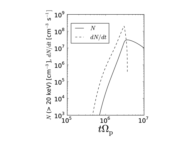
Figure 1: The number $N$ of electrons with energies $E$ exceeding 20 keV (solid line) and the acceleration rate $dN/dt$ in model solution A3. At $t=t_{\rm inj}$, wave injection ceases. Subsequently, the waves decay, and $N$ decreases because of Coulomb collisions.

In Figure 2 we plot the electron energy spectrum

$$N(E)=\frac{2\pi}{c^{2}}\,p\,\sqrt{p^{2}c^{2}+m^{2}_{\rm e}c^{4}}\,\int^{1}_{-1}d\mu\,f_{\rm e}(p,\mu),$$ (46)

in numerical calculation A3, where $\mu=p_{\parallel}/p$ and $E=\sqrt{p^{2}c^{2}+m^{2}_{\rm e}c^{4}}-m_{\rm e}c^{2}$. As this figure shows, a power-law-like structure develops over a narrow range of energies. At the end of the wave-injection period (i.e., at $t=t_{\rm inj}=3\times 10^{6}\mbox{ eV}$), this approximate power law extends from  $\sim 7\mbox{ keV}$ to $\sim 25\mbox{ keV}$, and $N(E)$ is roughly proportional to $E^{-3.3}$ in this range, shown in Figure 2. A similar power-law-like feature appears in Case 4 of MLM96 (their Figure 11). However, their approximate power law is much flatter than ours ($\sim E^{-\eta}$ with $\eta$ as small as 1.2) and extends to larger energies ($>100\mbox{ keV})$.

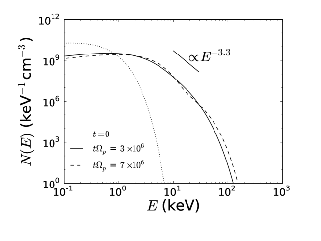
Figure 2: The electron energy spectrum $N(E)$ at three different times in model solution A3.

For reference, we carry out a fourth numerical calculation, A4, that is identical to A3, except that $E_{kz}$ is included. In this calculation, about 16% of the total energy injected into waves is transferred to electrons, which is about half as much as in solution A3. The values of $N_{20\rm max}$ and $R_{20\rm max}$ are $3.7\times 10^{6}$ and $2.0\times 10^{7}$ s^-1, respectively. These values are $\sim$ 8 times and 10 times smaller than those in solution A3. These reductions occur for the same reasons that the inclusion of $E_{kz}$ reduces the linear damping rate of fast waves in Maxwellian plasmas by a factor of 2 relative to the case in which $E_{kz}$ is neglected (Stix, 1992): the parallel electric force on electrons is $180^{\circ}$ degrees out of phase with the magnetic-mirror force, as discussed in Section 2.

5 Evolution of the Wave Power Spectrum $F_{k}$

In this section, we describe the characteristic way that $F_{k}$ evolves in our numerical calculations, using solutions A1 and A2 as examples. In Figure 3, we plot the energy-weighted average wavenumber

$$\langle k\rangle\equiv\frac{\int d^{3}k\;kF_{k}}{\int d^{3}k\;F_{k}}$$ (47)

for solution A2 (dashed line) and for a modified version of solution A2 in which transit-time damping is turned off (dash-dot-dash line). In this modified version of numerical calculation A2, the value of $\langle k\rangle$ is somewhat larger than in the original solution A2, consistent with the fact that TTD preferentially removes fast-wave energy at large $k$.

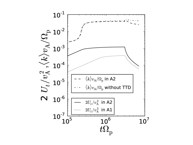
Figure 3: The total wave energy $U_{t}$ in model solution A2 (solid line) and solution A1 (dotted line). The dashed line is $\langle k\rangle$ in solution A2, and the dash-dot-dash line is $\langle k\rangle$ in a modified version of solution A2 in which transit-time damping is turned off.

In Figure 3 we also plot the total fast-wave fluctuation energy $U_{t}$ in numerical calculations A1 and A2. In Figure 4 we plot the angle-integrated, $k^{2}$-compensated power spectrum

$$E_{k}=2\pi\int_{0}^{\pi}d\theta\,\sin(\theta)k^{2}F_{k}$$ (48)

in numerical calculation A3 at three different times. At early times, $U_{t}$ grows, but this growth saturates while wave energy is still being injected. The reason for this saturation is that $F_{k}$ approaches a state in which energy injection at small $k$ is balanced by energy dissipation at large $k$. At early times, $\langle k\rangle$ also grows, as $F_{k}$ evolves towards a broad power-law-like spectrum. As can be seen in Figure 3, $U_{t}$ reaches its maximum value at an earlier time in solution A2 than in solution A1. This is because the larger values of $\dot{E}_{0}$ and $F_{k}$ in solution A2 reduce the energy cascade timescale at the forcing wavenumber $k_{0}$.

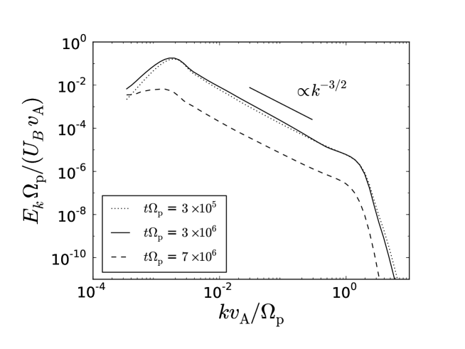
Figure 4: The angle-integrated, $k^{2}$-compensated fast-wave power spectrum $E_{k}$ at three different times in model solution A3.

As mentioned in Section 4, less than half of the energy that is injected into waves in all previously described numerical calculations is transferred to the electrons, and more than half cascades to $k>k_{\rm max}$ where it is dissipated by hyperviscosity. We note that much of the wave energy that cascades to $k>k_{\rm max}$ in our numerical calculations is in highly oblique waves with comparatively large values of $\sin\theta$. There are two reasons for this. As discussed in Section 2, the energy cascade time in fast-wave turbulence decreases as $\sin\theta$ increases. In addition, because of the TTD resonance condition, waves with $\sin\theta\sim 1$ interact with only a small number of high-speed electrons, and thus experience comparatively little damping.

6 The Anisotropic Electron Distribution Function

In this section, we focus on how resonant wave-particle interactions and Coulomb collisions affect the anisotropic electron distribution function. We begin with an example, solution B of Table 1, in which $t_{\rm inj}=\infty$, so that wave-injection is never shut off. Figure 5 shows $f_{\rm e}$ at three different times in this numerical calculation. In the middle and right panels of this figure, and at a fixed $p$, $f_{\rm e}$ peaks at a pitch angle corresponding approximately to the black line. (We discuss the precise way in which this black line is determined later in this section.) The electron distribution becomes increasingly anisotropic at higher energies, in the sense that the value of $p_{\parallel}/p_{\perp}$ along the black line increases as $p_{\parallel}$ increases. As we will argue in this section, the anisotropic structure of $f_{\rm e}$ reflects a balance between resonant interactions, which accelerates electrons to larger $|p_{\parallel}|$, and collisions, which isotropize the distribution. For reference, we plot the curve $p=p_{\rm T}$ (white quarter circles) in Figure 5, where

$$p_{\rm T}=\sqrt{2k_{B}m_{\rm e}T_{\rm e}}$$ (49)

is the thermal momentum.

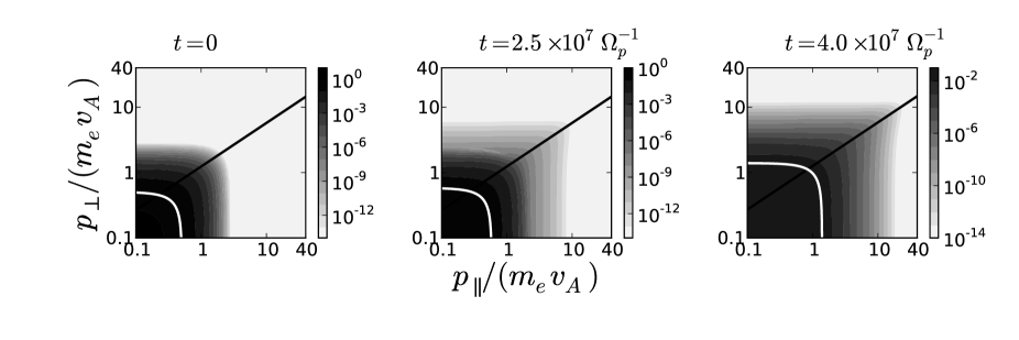
Figure 5: Grey-scale plot of the distribution function $f_{\rm e}$ in model solution B at $t=0$, $2.5\times 10^{7}\Omega^{-1}_{p}$, and $4.0\times 10^{7}\Omega^{-1}_{p}$. The solid lines are plots Equation (60), which represents the condition that the TTD timescale $\tau_{\rm ttd}$ equals the collisional timescale $\tau_{\perp\rm col}$.

To describe the interplay between wave-particle interactions and collisions analytically, we begin by obtaining an approximate analytic expression for the momentum diffusion coefficient $D_{\rm res}$ in Equation (23). Although some fast-wave energy at $k<k_{\rm max}=\Omega_{\rm p}/3v_{\rm A}$ is transferred to electrons via wave-particle interactions, we make the approximation that most of the fast-wave energy injected at small wavenumbers cascades to $k>k_{\rm max}$, as in the numerical calculations described in Section 4. We then model $F_{k}$ at $k<k_{\rm max}$ using weak-turbulence theory, neglecting losses of fast-wave energy due to wave-particle interactions. If fast-wave energy (per unit mass) is injected into the turbulence isotropically at small $k$ at rate $\dot{E}_{0}$ (i.e., $\sigma=1$ in (7)), then at $k_{0}\ll k<k_{\rm max}$

$$F_{k}=\left(\frac{4v_{\rm A}\dot{E}_{0}}{9\pi^{3}c_{2}}\right)\frac{k^{-7/2}}{\sin\theta},$$ (50)

where $c_{2}=\int_{0}^{\infty}dx\,\ln(1+x)[x(1+x)]^{-5/2}[(1+x)^{9/2}-x^{9/2}-1]\simeq 26.2$ (Chandran, 2005). We discuss Equation (50) further in Appendix C. We restrict our discussion to superthermal electrons, setting

$$p_{\perp}\gg p_{\perp\rm T},$$ (51)

which implies that TTD interactions dominate over LD interactions, as discussed following Equation (23). Upon substituting Equations (50) and (51) into Equation (23), we find that

$$D_{\rm res}\simeq D_{\rm ttd}$$ (52)

where

$$D_{\rm ttd}=\left(\frac{\pi}{9c_{2}}\right)^{1/2}\frac{m_{\rm e}^{2}\gamma^{2}v_{\perp}^{4}}{v_{\parallel}^{4}}\left[k_{\rm max}v_{\rm A}\dot{E}_{0}(v_{\parallel}^{2}-v_{\rm A}^{2})\right]^{1/2}$$ (53)

is the parallel-momentum diffusion coefficient arising from TTD interactions. We henceforth restrict our analysis to non-relativistic or trans-relativistic electrons, setting

$$\gamma\simeq 1.$$ (54)

The characteristic timescale on which TTD changes an electron’s parallel momentum by a factor of order unity is

$$\tau_{\rm ttd}\sim\frac{p_{\parallel}^{2}}{D_{\rm ttd}}.$$ (55)

We define the perpendicular (parallel) collisional timescale $\tau_{\perp\rm col}$ ($\tau_{\parallel\rm col}$) to be the characteristic time required for Coulomb collisions to change $p_{\perp}$ ($p_{\parallel}$) by a factor of order unity. At $p\gg p_{\rm T}$ and below the black line in Figure 5, $p_{\perp}\ll p_{\parallel}$. In this region, $p_{\perp}$ can change by a factor of order unity when an electron’s pitch angle changes by much less than one radian, which causes $\tau_{\perp\rm col}$ to be $\ll\tau_{\parallel\rm col}$. We can show from Equation (37) that when $p\gg p_{\rm T}$ and $|p_{\parallel}|\gg p_{\perp}$, the momentum diffusion coefficient for diffusion in $p_{\perp}$ is approximately

$$D_{\perp\rm col}\simeq\frac{\nu_{0}(m_{\rm e}v_{\rm A})^{3}}{2|p_{\parallel}|},$$ (56)

where

$$\nu_{0}=\frac{4\pi\Lambda e^{4}n_{\rm e}}{m_{\rm e}^{2}v_{\rm A}^{3}}$$ (57)

is the characteristic collision frequency for electrons with momentum $m_{\rm e}v_{\rm A}$. The perpendicular collision timescale is then

$$\tau_{\perp\rm col}\sim\frac{p_{\perp}^{2}}{D_{\perp\rm col}}.$$ (58)

The relative importance of TTD and collisions can be determined by comparing $\tau_{\rm ttd}$ and $\tau_{\perp\rm col}$. Since $D_{\rm ttd}\propto v^{4}_{\perp}$ for electrons with $\gamma\simeq 1$, and since Coulomb collisions become weaker as $v_{\perp}$ increases, $\tau_{\rm ttd}\ll\tau_{\perp\rm col}$ at sufficiently large $v_{\perp}$. When $\tau_{\rm ttd}\ll\tau_{\perp\rm col}$, electrons diffuse primarily in $p_{\parallel}$ rather than $p_{\perp}$, which explains why the contours of constant $f_{\rm e}$ are horizontal at large $p_{\perp}$ in Figure 5. On the other hand, at very small $p_{\perp}$, $\tau_{\perp\rm col}\ll\tau_{\rm ttd}$ and electrons diffuse in $\ln(p_{\perp}/p_{\rm T})$ much more rapidly than they diffuse in $\ln(p_{\parallel}/p_{\rm T})$. This explains why the contours of constant $f_{\rm e}$ are nearly vertical at small $p_{\perp}$ in Figure 5.

The transition between the TTD-dominated regime at large $p_{\perp}$ and the collision-dominated regime at small $p_{\perp}$ occurs when

$$\tau_{\rm ttd}\sim\tau_{\perp\rm col}.$$ (59)

If we set $\tau_{\rm ttd}=\tau_{\perp\rm col}$, take $|p_{\parallel}|$ to be $\gg m_{\rm e}v_{\rm A}$, and replace the $\sim$ signs in Equations (55) and (58) with equals signs, we obtain

$$\frac{p_{\perp}}{m_{\rm e}v_{\rm A}}=1.3c_{3}\left(\frac{v_{\rm A}\nu_{0}^{2}}{k_{\rm max}\dot{E}_{0}}\right)^{1/12}\left(\frac{p_{\parallel}}{m_{\rm e}v_{\rm A}}\right)^{2/3},$$ (60)

where $c_{3}$ is a dimensionless constant, which we have inserted to account for the uncertainties in replacing the $\sim$ signs with $=$ signs. The black lines in Figure 5 are plots of Equation (60) with

$$c_{3}=0.89.$$ (61)

As mentioned previously, at a fixed $p>p_{\rm T}$, $f_{\rm e}$ reaches its maximum value close to the black lines in Figure 5. To a reasonable approximation, we can thus take the majority of the electrons at any fixed non-thermal energy $E$ to satisfy Equation (60) to within a factor of order unity. In this approximation, we can view all properties of the non-thermal electrons as functions of the single variable $p_{\parallel}$. For example, $p_{\perp}=p_{\perp}(p_{\parallel})$, $\tau_{\rm ttd}=\tau_{\rm ttd}(p_{\parallel})$, etc. The way that electrons diffuse out to larger energies along the black lines in Figure 5 is through a combination of two processes. TTD causes electrons to diffuse in $p_{\parallel}$ at a fixed $p_{\perp}$, and Coulomb collisions scatter electrons to larger values of $p_{\perp}$. If we focus on one of the horizontal lines of constant $f_{\rm e}$ above the black lines in Figure 5, the timescale $\tau_{\rm ttd}$ increases as $p_{\parallel}$ increases. The time it takes an electron to reach a point on one of the black lines in Figure 5 with parallel velocity $p_{\parallel}$ is thus $\sim\tau_{\rm ttd}(p_{\parallel})$, or equivalently $\tau_{\perp\rm col}(p_{\parallel})$. This timescale is the acceleration timescale, denoted $\tau_{\rm acc}$:

$$\tau_{\rm acc}(p_{\parallel})=\tau_{\perp\rm col}(p_{\parallel}).$$ (62)

With the use of Equations (56), (58), and (60), we find that

$$\tau_{\rm acc}=3.4c_{3}^{2}\left(\frac{v_{\rm A}}{\nu_{0}^{4}\,k_{\rm max}\dot{E}_{0}}\right)^{1/6}\left(\frac{p_{\parallel}}{m_{\rm e}v_{\rm A}}\right)^{7/3}.$$ (63)

The largest $|p_{\parallel}|$ to which an electron can be accelerated, denoted $p_{\parallel\rm max}$, is approximately given by the condition

$$\tau_{\rm acc}(p_{\parallel\rm max})=\Delta t,$$ (64)

where

$$\Delta t=t-\tau_{\rm cas}$$ (65)

is the duration of the acceleration process. The values of the energy cascade timescale $\tau_{\rm cas}$ (defined in Equation (9)) in our numerical calculations are listed in Table 1. (We note that at $0<t<t_{\rm cas}$, $F_{k}$ is still growing, and Equation (53), which is the basis of our analysis, does not apply.) Equation (64) leads to a maximum parallel momentum of

$$p_{\parallel\rm max}=0.59c_{3}^{-6/7}\nu_{0}^{2/7}\left(\frac{k_{\rm max}\dot{E}_{0}}{v_{\rm A}}\right)^{1/14}\left(\Delta t\right)^{3/7}m_{\rm e}v_{\rm A}.$$ (66)

In the $\gamma\simeq 1$ limit that we have been focusing on, the maximum energy $E_{\rm max}$ that electrons can be accelerated to via TTD is then

$$E_{\rm max}\simeq\frac{[p_{\perp}(p_{\parallel\rm max})]^{2}+p_{\parallel\rm max}^{2}}{2m_{\rm e}}$$ (67)

We note that Equations (66) and (67) are valid only when $t_{\rm cas}<t<t_{\rm inj}$. At larger values of $t$, after wave injection ceases, the fast-wave energy decays away, TTD interactions cease, and the electrons undergo a purely collisional evolution, which is described further in Section 7.

Referring to Figure 2, the energy $E_{\rm max}$ is the high-energy cutoff of the non-thermal tail in the electron energy distribution. We now discuss, with the aid of Figure 6, the physics that determines the minimum energy of this non-thermal tail, which we denote $E_{\rm nt}$, again restricting our discussion to $t<t_{\rm inj}$. The vertical dashed line Figure 6 represents the minimum parallel momentum $p_{\parallel}=m_{\rm e}v_{\rm A}$ at which electrons can satisfy the TTD resonance condition, Equation (2).

The solid line in this figure is a plot of the solution of Equation (60) for some arbitrary choice of parameters. Above this line, and to the right of the dashed line, $\tau_{\rm ttd}<\tau_{\perp\rm col}$ and TTD interactions are dominant. That is, electrons diffuse primarily in $p_{\parallel}$ rather than in $p_{\perp}$, as illustrated schematically with the horizontal double-headed arrow. The $p_{\perp}$ coordinate at the intersection of the solid and dashed lines is denoted $p_{\perp\rm min}$ and is the minimum value of $p_{\perp}$ for which TTD can dominate over collisions. Assuming that $E<E_{\rm max}$, electrons with $p_{\perp}>p_{\perp\rm min}$ diffuse rapidly in $p_{\parallel}$ within the interval $p_{\parallel}\in[m_{\rm e}v_{\rm A},p_{\parallel}(p_{\perp})]$, where the function $p_{\parallel}(p_{\perp})$ is obtained by inverting Equation (60). In the non-relativistic limit, the energies at the endpoints of this $p_{\parallel}$ interval are

$$E_{1}(p_{\perp})=\frac{1}{2m_{\rm e}}\left(p^{2}_{\perp}+m^{2}_{\rm e}v^{2}_{\rm A}\right)$$ (68)

and

$$E_{2}(p_{\perp})=\frac{1}{2m_{\rm e}}\left\{p^{2}_{\perp}+[p_{\parallel}(p_{\perp})]^{2}\right\}.$$ (69)

These endpoints are labeled $E_{1}$ and $E_{2}$ in Figure 6. We define the ratio

$$R(p_{\perp})=\frac{N_{\rm M}(E_{1})}{N_{\rm M}(E_{2})},$$ (70)

where $N_{\rm M}(E)$ is the Maxwellian energy spectrum, obtained by replacing $f_{\rm e}$ in Equation (46) with $f_{\rm M}$, the Maxwellian distribution that has the same total energy as the instantaneous value of $f_{\rm e}$. When $p_{\perp}$ is just slightly larger than $p_{\perp\rm min}$, $E_{1}$ and $E_{2}$ are not too dissimilar, $R(p_{\perp})$ is not very large, and the diffusion of electrons from $p_{\parallel}=m_{\rm e}v_{\rm A}$ to $p_{\parallel}=p_{\parallel}(p_{\perp})$ causes only a minor enhancement of the energy spectrum at $E=E_{2}$ relative to a Maxwellian energy spectrum. Such a minor enhancement is unable to produce a noticeable non-thermal tail in $N(E)$. However, as $p_{\perp}$ increases, $R(p_{\perp})$ grows, and eventually the diffusion of electrons from $p_{\parallel}=m_{\rm e}v_{\rm A}$ to $p_{\parallel}=p_{\parallel}(p_{\perp})$ produces a major enhancement in the value of $N(E)$ at $E=E_{2}$, leading to the presence of a substantial non-thermal tail in the distribution. In our numerical calculations, we find that the non-thermal tail begins at an energy $\sim E_{2}(p_{\perp\rm nt})$, where $p_{\perp\rm nt}$ is the solution of the equation

$$R(p_{\perp\rm nt})=100.$$ (71)

That is,

$$E_{\rm nt}=E_{2}(p_{\perp\rm nt}).$$ (72)

Figure 6: The solid line is the solution to Equation (60) for some arbitrary choice of parameters. This line gives the location in the $(p_{\parallel},p_{\perp})$ plane at which $\tau_{\rm ttd}=\tau_{\perp\rm col}$. The vertical dashed line $p_{\parallel}=m_{\rm e}v_{\rm A}$ shows the minimum $p_{\parallel}$ for which electrons can undergo resonant TTD interactions. The horizontal dotted line represents $p_{\parallel}$-diffusion due to TTD, which dominates over collisions above the solid line and to the right of the dashed line. In order for TTD to be dominant, $p_{\perp}$ must exceed $p_{\perp\rm min}$, which is the $p_{\perp}$ coordinate of the intersection between the solid and dashed lines. The energies $E_{1}(p_{\perp})$ and $E_{2}(p_{\perp})$ are evaluated, respectively, along the dashed and solid lines.

Qualitatively, there are two main factors that control the value of $E_{\rm nt}$. The first is the amplitude of the fast-wave turbulence. As $\dot{E}_{0}$ and $F_{k}$ decrease, $p_{\perp\rm min}$ increases, since electrons need larger values of $p_{\perp}$ for TTD to dominate over collisions. This causes $E_{\rm nt}$ to increase as a consequence. On the other hand, if $\dot{E}_{0}$ and $F_{k}$ are sufficiently large, $E_{\rm nt}$ can be reduced to energies just moderately above the thermal energy. The second factor that influences $E_{\rm nt}$ is the electron temperature. As electrons are heated, the effects of TTD on $f_{\rm e}$ become pronounced only at higher and higher electron energies, causing $E_{\rm nt}$ to increase. For example, if at a fixed $p_{\perp}$, the difference in the energy between the dashed line and solid line in Figure 6 is less than $k_{\rm B}T_{\rm e}$, then the diffusion of electrons from $p_{\parallel}=m_{\rm e}v_{\rm A}$ to $p_{\parallel}=p_{\parallel}(p_{\perp})$ at that value of $p_{\perp}$ will have only a minor effect on $N(E_{2}(p_{\perp}))$. We note that the location of the black solid lines in Figures 5 and 6 do not depend upon $T_{\rm e}$, since $T_{\rm e}$ does not enter into Equation (60).

In Figures 7 and 8, we compare our expressions for $E_{\rm max}$ and $E_{\rm nt}$ in Equations (67) and (72) with the electron energy spectrum in model solution B at three different times. We show the same comparison for two snapshots of solutions C and D in Figure 9. For the most part, our expressions for $E_{\rm max}$ and $E_{\rm nt}$ in Equations (67) and (72) approximately bound the non-thermal tail in the electron distribution in our numerical calculations. The least successful fit occurs in solution C, for which Equation (67) underestimates $E_{\rm max}$ by a factor of $\sim 2$. A discrepancy of this magnitude, however, is not entirely surprising, given the approximations we have made in deriving Equation (67).

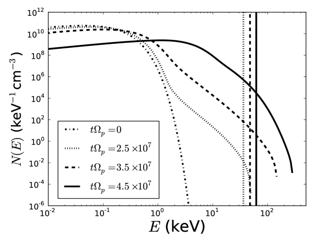
Figure 7: The electron energy spectrum $N(E)$ in model solution B at $t=0$, $2.5\times 10^{7}\Omega^{-1}_{p}$, $3.5\times 10^{7}\Omega^{-1}_{p}$, and $4.5\times 10^{7}\Omega^{-1}_{p}$. The dotted, dashed, and solid vertical lines indicate the values of $E_{\rm max}$ from Equation (67) at $t=2.5\times 10^{7}\Omega^{-1}_{p}$, $t=3.5\times 10^{7}\Omega^{-1}_{p}$, and $t=4.5\times 10^{7}\Omega^{-1}_{p}$, respectively.

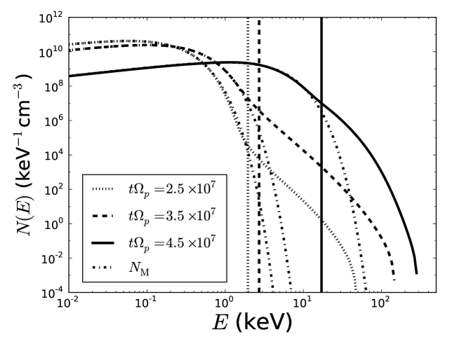
Figure 8: The dotted-line, dashed-line, and solid-line curves are plots of $N(E)$ in model solution B at $t=2.5\times 10^{7}\Omega^{-1}_{p}$, $t=3.5\times 10^{7}\Omega^{-1}_{p}$, and $t=4.5\times 10^{7}\Omega^{-1}_{p}$, respectively. The dash-dot-dash curves are Maxwellian energy spectra $N_{\rm M}(E)$ that have the same total energy as $N(E)$ at these same three times. The vertical dotted, dashed, and solid lines show the values of $E_{\rm nt}$ at the times $t=2.5\times 10^{7}\Omega^{-1}_{p}$, $t=3.5\times 10^{7}\Omega^{-1}_{p}$, and $t=4.5\times 10^{7}\Omega^{-1}_{p}$, respectively.

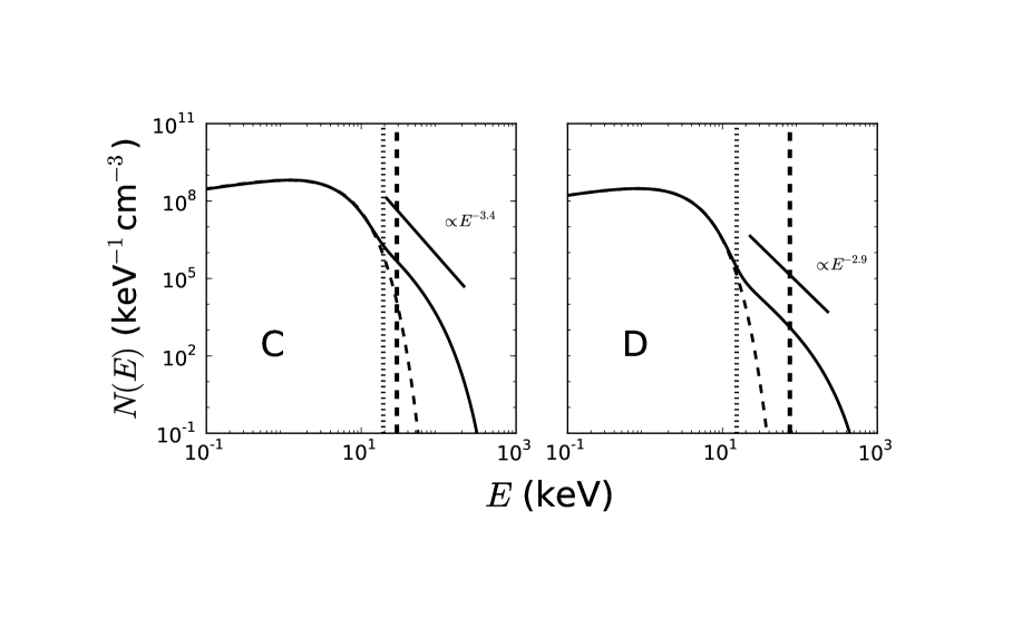
Figure 9: Solid-line curves are $N(E)$ in model solution C at $t=2.8\times 10^{7}\Omega^{-1}_{p}$ (left panel) and solution D at $t=2\times 10^{8}\Omega^{-1}_{p}$ (right panel). The thin dashed lines are plots of Maxwellian distributions with the same total energy as the (non-Maxwellian) electron spectra. The vertical dotted (thick-dashed) lines show the locations of $E_{\rm nt}$ ($E_{\rm max}$) in these numerical calculations at these same times. At the moments, the spectral indices are $3.4$ and $2.9$ from the solutions C and D, respectively. The straight solid lines are power-law fits to $N(E)$ in the energy interval $E_{\rm nt}<E<E_{\rm max}$.)

6.1 The Minimum $\beta_{\rm e}$ Required for Efficient TTD

The fraction of the electron population that is significantly affected by TTD depends strongly on $\beta_{\rm e}$. If $\beta_{\rm e}\ll m_{\rm e}/m_{\rm p}$, then the electron thermal speed is much less than $v_{\rm A}$, and the number of electrons with $|p_{\parallel}|\gg m_{\rm e}v_{\rm A}$ is exponentially small. Since $|p_{\parallel}|$ must exceed $m_{\rm e}v_{\rm A}$ in order for electrons to satisfy the TTD resonance condition, TTD interactions with fast waves are exceedingly weak if $\beta_{\rm e}\ll m_{\rm e}/m_{\rm p}$.

If $\beta_{\rm e}$ is initially small compared to $m_{\rm e}/m_{\rm p}$ in a flare, there may be a transient early stage in a flare in which some process heats the electrons until $\beta_{\rm e}\sim m_{\rm e}/m_{\rm p}$. During this initial heating stage, TTD is ineffective at accelerating electrons to non-thermal energies since only a minuscule fraction of the electrons have $p_{\parallel}>m_{\rm e}v_{\rm A}$. However, after this heating stage, a significant fraction of electrons satisfy $p_{\parallel}>m_{\rm e}v_{\rm A}$, and TTD acceleration to higher energies becomes much more efficient.

6.2 Power-Law Fits to the Non-thermal Tail

TTD results in a non-thermal tail in the electron energy spectrum that resembles a power law within the energy range $E_{\rm min}<E<E_{\rm max}$. We fit the energy spectra in our numerical calculations within this energy range with a power-law of the form $N(E)\propto E^{-\eta}$ and show these fits in Figures 2, 9, and 10. The resulting values of $\eta$ range from $2.9$ to $3.4$. As mentioned in Section 4, our electron energy spectra are steeper than in the isotropic-$f_{\rm e}$ model of Miller et al. (1996), in which the non-thermal tail in $N(E)$ can scale like $E^{-\eta}$ with eta as small as 1.2.

7 Time Evolution of the Electron Energy Spectrum

In Figure 10 we plot the electron energy spectrum $N(E)$ at different times in model solution D. Between $t=0$ and $t\sim 42\mbox{ s}$, the electron distribution develops a non-thermal, power-law-like tail extending to $\sim 80\mbox{ keV}$. As time progresses, this power-law tail shifts to larger energies, and the temperature of the thermal particles increases, so that the thermal distribution shifts into the energy window shown in the figure. After wave injection ceases at $t=t_{\rm inj}=$ 3 min 23 s, the heating of the thermal distribution ends, and the non-thermal particles are gradually pulled back into the thermal distribution by Coulomb collisions. However, the collision frequency is $\propto p^{-3}$ at these non-thermal energies, and thus the low-energy end of the non-thermal tail is affected by collisions earlier than the high-energy end is affected. As a result, during the collisional evolution at $t>t_{\rm inj}$, the non-thermal tail drops to lower amplitudes but becomes flatter, as can be seen in the middle and right panels of Figure 10.

The evolution of $N(E)$ shown in Figure 10 is qualitatively similar to the evolution of the hard x-ray spectrum observed in the June 27, 1980 flare, which is plotted in Figure 3 of Lin et al. (1981). In both our model and the observations: (1) the power-law part of the spectrum is confined to a fairly narrow energy range, with $N(E)$ steepening at $E\sim 100\mbox{ keV}$; (2) the thermal distribution and non-thermal tail shift to higher energies as time progresses during the early stages of the flare; and (3) during the late stages of the flare, the non-thermal tail becomes flatter, but drops in amplitude.

Although the electron spectrum in solution D qualitatively resembles the photon spectrum in the June 27, 1980 flare, our model is not yet sufficiently sophisticated to produce a synthetic hard x-ray spectrum $I(E)$ for a detailed comparison to the observations. In order for us to map $N(E)$ in our model, which is the electron energy spectrum in the coronal acceleration region, into an x-ray spectrum $I(E)$, we would need to calculate the flux of electrons per unit energy $F(E)$ into the chromosphere, and we would need to account for the way that the escape of particles from the corona modifies $N(E)$.

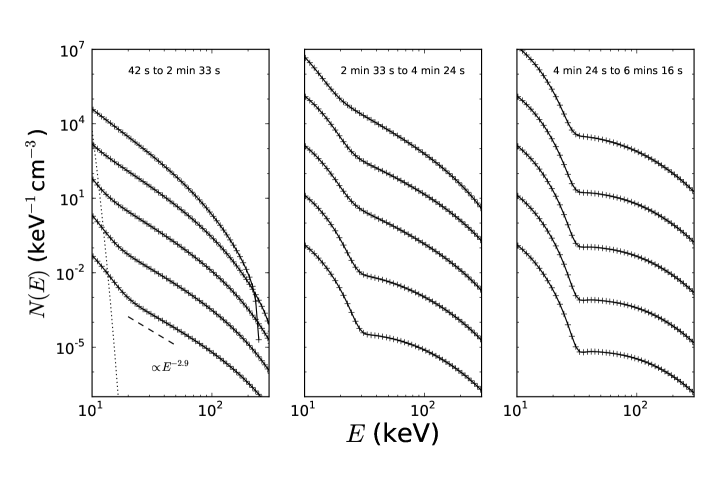
Figure 10: The time evolution of the electron energy spectrum $N(E)$ in model solution D. The dotted-line curve in the left panel is the initial Maxwellian spectrum at $t=0$ s. The curves plotted with $+$ signs in all three panels are plots of $N(E)$ at $t=(42+27.75j)\mbox{ s}$ with $j=0,1,2,...12$. These curves are ordered in time, from top to bottom in each panel, with $j\in(0,4)$ in the left panel, $j\in(4,8)$ in the middle panel, and $j\in(9,12)$ in the right panel. The scale on the vertical axis applies to the topmost $+$-sign curve in each panel as well as the dotted line in the left panel, with each succeeding plot of $N(E)$ in each panel offset downward by a factor of $10^{-2}$.

8 Discussion and Conclusion

In this paper, we develop a stochastic-particle-acceleration (SPA) model in which electrons are energized by weakly turbulent fast magnetosonic waves via a combination of transit-time-damping (TTD) interactions, Landau-damping (LD) interactions, and pitch-angle scattering from Coulomb collisions. We use quasilinear theory and weak turbulence theory to describe the time evolution of the electron distribution function $f_{\rm e}$ and the fast-wave power spectrum $F_{k}$. We solve the equations of this model numerically and find that TTD leads to power-law-like non-thermal tails in the electron energy spectrum $N(E)$ extending from a minimum energy $E_{\rm nt}$ to a maximum energy $E_{\rm max}$. We derive approximate analytic expressions for $E_{\rm nt}$ and $E_{\rm max}$ and find that these expressions agree with our numerical solutions reasonably well. For a fast wave, the parallel electric field exerts a force on electrons that is $180^{\circ}$ out of phase with the magnetic-mirror force, and thus the inclusion of the parallel electric field (LD interactions) in our model reduces the rate of electron acceleration (see, e.g., the discussion of numerical calculation A4 at the end of Section 4).

The main new feature of our model that distinguishes it from previous studies is our inclusion of anisotropy in both momentum space and wavenumber space. We assume cylindrical symmetry about the magnetic field direction in both velocity space and wavenumber space, but allow $f_{\rm e}$ to depend upon both $p_{\perp}$ and $p_{\parallel}$ and $F_{k}$ to depend on both $k_{\perp}$ and $k_{\parallel}$. Another new feature of our work in the context of SPA models is our use of weak turbulence theory to describe the fast-wave energy cascade, which enables us to avoid introducing an adjustable free parameter into the energy cascade rate and to account for the weakening of the energy cascade as $\sin\theta$ decreases, where $\theta$ is the angle between the wavevector $\bm{k}$ and the background magnetic field $\bm{B}_{0}$.

To investigate how much these new features affect our results, we compare one of our numerical solutions with a numerical example (“Case 4”) published by Miller et al. (1996) (MLM96), which is based on their isotropic SPA model. We find that there are two main differences between our model and theirs. The first concerns the energy cascade rate. They modeled the fast-wave energy cascade by solving a nonlinear diffusion equation for $F_{k}$, in which the diffusion coefficient contained an adjustable free parameter. If we set the injection rate to produce $k^{2}F_{k}=Ak^{-3/2}$ in both models, where $A$ is some constant, then the energy cascade rate in our model is roughly 9 times faster than in their model. Conversely, if we set the energy cascade rates to be equal in the two models, then $F_{k}$ is smaller in our model than in theirs by a factor of $\simeq 3$, which weakens electron acceleration by fast waves in our model relative to theirs. The second main difference between the two models is that the anisotropy of $f_{\rm e}$ reduces the efficiency of electron acceleration via TTD. This is because TTD accelerates electrons to larger values of $|p_{\parallel}|$, but not to larger values of $p_{\perp}$, which causes most of the electrons in our model to satisfy $|p_{\parallel}|>p_{\perp}$. The TTD momentum diffusion coefficient $D_{\rm ttd}$ for energetic electrons (with $|v_{\parallel}|\gg v_{\rm A}$), however, is $\propto\gamma^{2}v_{\perp}^{4}/|v_{\parallel}|^{3}$, and the electrons in our anisotropic model thus have smaller values $D_{\rm ttd}$ than in MLM96’s isotropic model. Because of these differences, the total number of electrons accelerated to energies $>20\mbox{ keV}$ is smaller in our model than in MLM96’s, the power-law-like non-thermal tails in the electron energy spectrum are steeper in our model, and these tails are limited to lower maximum energies in our model.

Beyond the comparison with MLM96, our principal results are the following:

1. In the presence of TTD and Coulomb collisions, the electron distribution function at non-thermal energies approaches a specific characteristic form, which is shown in Figure 5. At a fixed $p$, $f_{\rm e}$ peaks at a pitch angle that corresponds to the black line in Figure 5. This line is a plot of Equation (60) and corresponds to the locations in the $p_{\perp}$-$p_{\parallel}$ plane at which the TTD timescale $\tau_{\rm ttd}$ equals the collisional timescale $\tau_{\perp\rm col}$. Above this black line (at large $p_{\perp}$), TTD dominates over collisions, and rapid $p_{\parallel}$-diffusion of electrons causes $f_{\rm e}$ to become almost independent of $p_{\parallel}$. Below this curve, collisions dominate over TTD, and $f_{\rm e}$ depends more strongly on $\ln p_{\parallel}$ than on $\ln p_{\perp}$.

2. As can be seen in our expression for $E_{\rm max}$ in Equation (67), the maximum energy of the non-thermal tail increases with increasing electron density $n_{\rm e}$. This is because collisions help electrons to reach higher energies by converting some of the parallel kinetic energy ($m_{\rm e}v_{\parallel}^{2}/2$) gained via TTD interactions into perpendicular kinetic energy ($m_{\rm e}v_{\perp}^{2}/2$), which increases the rate of TTD acceleration (since $D_{\rm ttd}\propto\gamma^{2}v_{\perp}^{4}/|v_{\parallel}|^{3}$ for energetic electrons). Another way of thinking about this is that an electron can only reach a point $(p_{\parallel},p_{\perp})$ on the black line in Figure 5 after the elapsed time $\Delta t$ has grown to a value of order the collisional timescale $\tau_{\perp\rm col}$ at that point (which equals the TTD timescale $\tau_{\rm ttd}$ at that point). Consistent with this reasoning, $E_{\rm max}$ increases with $t$ up until the wave injection ceases and the waves decay away.

3. One of the ways that the magnetic field strength $B_{0}$ and the initial electron temperature affect electron acceleration via TTD is through their influence on the value of $\beta_{\rm e}$. If the initial value of $\beta_{\rm e}$ is $\ll m_{\rm e}/m_{\rm p}$, then only an exponentially small fraction of the electrons have large enough values of $|v_{\parallel}|$ that they can satisfy the TTD resonance condition Equation (2), and TTD acceleration is exceedingly weak.

4. The time evolution of $N(E)$ in our model solution D qualitatively resembles the time evolution of the hard x-ray spectrum $I(E)$ in the June 27, 1980 flare reported by Lin et al. (1981). However, our model is not yet sophisticated enough to produce synthetic x-ray spectra, because we have neglected the escape of electrons from the acceleration region, which alters $N(E)$ and is needed to determine $I(E)$.

There are several processes that we have not included in our model. As just mentioned, we have not accounted for the escape of electrons from the flare acceleration region or the flow of low-energy electrons into the acceleration region from the chromosphere. We have also neglected the escape of fast waves from the acceleration region (see Pongkitiwanichakul et al. (2012) for a detailed discussion of wave escape) and resonance broadening in wave-particle interactions (Shalchi et al., 2004; Shalchi & Schlickeiser, 2004; Yan & Lazarian, 2008; Lynn et al., 2012, 2013, 2014). In the numerical calculations we have carried out so far, a significant amount of the power injected into fast waves at small $k$ cascades to $k>\Omega_{\rm p}/v_{\rm A}$, where it presumably initiates a cascade of whistler waves. However, our model neglects the effects of whistler waves and other waves at $k\gtrsim\Omega_{\rm p}/v_{\rm A}$ on the electrons. A related point is that we have neglected non-collisional forms of pitch-angle scattering. One of the effects that waves at $k>\Omega_{\rm p}/v_{\rm A}$ could have is to enhance the electron pitch-angle scattering rate. By converting perpendicular electron kinetic energy into parallel kinetic energy, such enhanced pitch-angle scattering would increase the efficiency of TTD electron acceleration in flares.

A useful direction for future research would be to incorporate some or all of these processes into the type of anisotropic SPA model that we have developed. Another valuable direction for future research would be to determine the amplitude of fast-wave turbulence in solar flares using large-scale direct numerical simulations. Because the turbulence amplitude plays a critical role in SPA models, a determination of this amplitude would lead to much more rigorous tests of SPA models than have previously been possible.

Appendix A Analytic Expression for the Wave Damping Rate Allowing for Relativistic Particles

We follow the standard approach in quasilinear theory of treating the plasma as infinite and homogeneous. To obtain Fourier transforms of the fluctuating quantities, we define the “windowed” Fourier transform

$$\tilde{g}(\bm{k})=\frac{1}{(2\pi)^{3}}\int d^{3}x\,\,g(\bm{x})H(\bm{x})\exp{(-i\bm{k}\cdot\bm{x})},$$ (A1)

where

$$H(\bm{x})=\left\{\begin{array}[]{cc}\displaystyle 1&\mbox{ if $|x|<\displaystyle\frac{L}{2}$, $|y|<\displaystyle\frac{L}{2}$, and $|z|<\displaystyle\frac{L}{2}$ }\vspace{0.2cm}\\ 0&\mbox{otherwise}\end{array}\right..$$ (A2)

As mentioned in Section 2, our Fourier-transform convention is the same as that of Stix (1992), except that we have an extra factor of $(2\pi)^{-3/2}$ on the right-hand side of Equation (A1). Accounting for this difference, we can use Eq. (67) of Chapter 4 of Stix (1992) to write the wave energy density $\epsilon_{w}$ in the form

$$\varepsilon_{w}=\lim_{L\rightarrow\infty}\left(\frac{2\pi}{L}\right)^{3}\int d^{3}k\,2W_{k},$$ (A3)

where $W_{k}$ is defined in Equation (25).

Wave-particle interactions cause the particle kinetic energy density of species $s$ to change at the rate

$$\dot{K}_{s}=\int d^{3}p\,\,[(p^{2}c^{2}+m^{2}_{s}c^{4})^{1/2}-m_{s}c^{2}]\left(\frac{\partial f_{s}}{\partial t}\right)_{\rm res},$$ (A4)

where $(\partial f_{s}/\partial t)_{\rm res}$ is given in Equation (2). The second term in brackets in Equation (A4), $m_{s}c^{2}$, can be dropped, because $\int d^{3}p(\partial f_{s}/\partial t)_{\rm res}=0$. Equation (A3) implies that wave-particle interactions cause the wave energy density to change at the rate

$$\dot{\varepsilon}_{w}=\left(\frac{2\pi}{L}\right)^{3}\int d^{3}k\,4\gamma_{k}W_{\bm{k}},$$ (A5)

where $\gamma_{k}$ is the imaginary part of the wave frequency. Because the sum of the wave and particle-kinetic-energy densities is conserved,

$$\sum_{s}\dot{K}_{s}+\dot{\varepsilon}_{w}=0.$$ (A6)

Upon substituting Equation (2) into the right-hand side of Equation (A4), integrating by parts, and using the identity

$$\frac{\partial v_{\perp}}{\partial p_{\parallel}}=\frac{\partial v_{\parallel}}{\partial p_{\perp}},$$ (A7)

we can rewrite Equation (A6) in the form

$$\int d^{3}kW_{k}I_{k}=0,$$ (A8)

where

$$I_{k}=\gamma_{k}-\sum_{s}\sum_{n=-\infty}^{\infty}\frac{\pi^{2}q_{s}^{2}}{2}\int_{0}^{\infty}dp_{\perp}\int_{-\infty}^{\infty}dp_{\parallel}\frac{p_{\perp}^{2}c^{2}}{\sqrt{p^{2}c^{2}+m_{s}^{2}c^{4}}}\frac{|\psi_{n,k}^{(s)}|^{2}}{W_{k}}\delta(\omega_{kr}-k_{\parallel}v_{\parallel}-n\Omega_{s})Gf_{s}.$$ (A9)

Equation (A8) must be satisfied for any function $W_{k}$, and hence $I_{k}$ must vanish at all $k$. The condition that $I_{k}=0$ at each $k$ reflects the fact that the change in the energy of the waves within any small volume $V$ of wavenumber space is equal and opposite to the change in the particle kinetic energy that results from wave-particle interactions involving waves with $\bm{k}\in V$. We make use of this fact when we evaluate $\gamma_{k}$ in our numerical calculations. Specifically, when we evaluate $(\partial f_{\rm e}/\partial t)_{\rm res}$, we keep track of the change in particle kinetic energy that results from interactions with waves within each grid cell in wavenumber space. We use the term $\Delta K_{i}$ to denote the change in particle kinetic energy resulting from waves in the $i^{\rm th}$ grid cell. We then evaluate $\gamma_{k}$ within the $i^{\rm th}$ cell by setting $(2\pi/L)^{3}4\gamma_{k}W_{k}(\Delta k)_{i}^{3}\Delta t$ within that cell equal to $-\Delta K_{i}$, where $(\Delta k)_{i}^{3}$ is the volume of the grid cell in $k$ space, and $\Delta t$ is the time step. By using this procedure, we ensure that the changes in $f_{\rm e}$ and $F_{k}$ that result from wave-particle interactions conserve energy to machine accuracy.

From the equation $I_{k}=0$, we obtain

$$\gamma_{k}=\sum_{s}\sum_{n=-\infty}^{\infty}\frac{\pi^{2}q_{s}^{2}}{2}\int_{0}^{\infty}dp_{\perp}\int_{-\infty}^{\infty}dp_{\parallel}\frac{p_{\perp}^{2}c^{2}}{\sqrt{p^{2}c^{2}+m_{s}^{2}c^{4}}}\frac{|\psi_{n,k}^{(s)}|^{2}}{W_{k}}\delta(\omega_{kr}-k_{\parallel}v_{\parallel}-n\Omega_{s})Gf_{s}.$$ (A10)

In the non-relativistic limit, Equation (A10) can be written in the form

$$\gamma_{\bm{k}}=\sum_{s}\sum_{n=-\infty}^{\infty}\frac{\pi\omega^{2}_{ps}}{8n_{\rm e}}\left|\frac{1}{k_{\|}}\right|\int^{\infty}_{0}dv_{\perp}v^{2}_{\perp}\int^{\infty}_{-\infty}dv_{\parallel}\frac{|\psi_{n,\bm{k}}^{(s)}|^{2}}{W_{\bm{k}}}\delta\left(v_{\|}-\frac{\omega_{kr}-n\Omega}{k_{\|}}\right)G_{v}f_{s}^{(v)},$$ (A11)

where $\omega_{ps}=\sqrt{4\pi n_{s}q_{s}^{2}/m_{s}}$ is the plasma frequency of species $s$, $f_{s}^{(v)}=f_{s}/m_{\rm e}^{3}$ is (in the non-relativistic limit) the usual velocity-space distribution function, and

$$G_{v}=\left(1-\frac{k_{\parallel}v_{\parallel}}{\omega_{kr}}\right)\frac{\partial}{\partial v_{\perp}}+\left(\frac{k_{\parallel}v_{\perp}}{\omega_{kr}}\right)\frac{\partial}{\partial v_{\parallel}}.$$ (A12)

Equation (A11) is exactly the result derived by Kennel & Wong (1967). Equation (A10) can thus be viewed as a generalization of Kennel & Wong’s (1967) result that allows for relativistic particles.

Appendix B Estimating the Error in our Approximate Collision Operator

The Coulomb collision operator involves the quantities

$$K_{1}(\bm{p})=\int d^{3}p^{\prime}f_{\rm e}(\bm{p}^{\prime})u^{-1},$$ (B1)

and

$$K_{2}(\bm{p})=\int d^{3}p^{\prime}f_{\rm e}(\bm{p}^{\prime})u,$$ (B2)

where $u=|\bm{p}^{\prime}-\bm{p}|$. To evaluate these integrals would require a very large number of operations per time step. In order to increase the speed of the calculations, we replace $K_{1}(\bm{p})$ and $K_{2}(\bm{p})$, respectively, with

$$H_{1}(\bm{p})=\int d^{3}p^{\prime}f_{\rm M}(\bm{p}^{\prime})u^{-1}$$ (B3)

and

$$H_{2}(\bm{p})=\int d^{3}p^{\prime}f_{\rm M}(\bm{p}^{\prime})u,$$ (B4)

where $f_{\rm M}$ is the Maxwellian distribution that has the same total particle kinetic energy as $f_{\rm e}$. In this case, $H_{1}(\bm{p})$ and $H_{2}(\bm{p})$ can be pre-calculated and depend only on $p_{\perp}$, $p_{\parallel}$, $n_{\rm e}$, and $T_{\rm e}$.

To estimate the error introduced by this approximation we compare $H_{1}(\bm{p})$ to $K_{1}(\bm{p})$ and $H_{2}(\bm{p})$ to $K_{2}(\bm{p})$ in numerical calculations A3, B, C, and D. The maximum values of $|H_{1}-K_{1}|/K_{1}$ and $|H_{2}-K_{2}|/K_{2}$ increase as $f_{\rm e}$ deviates from a Maxwellian shape. They increase and reach their maximum value approximately at $t=t_{\rm inj}$. In model solutions A3 and D, which have finite injection times, the maximum values of $|H_{1}-K_{1}|/K_{1}$ are 0.06 and 0.004, and the maximum values of $|H_{2}-K_{2}|/K_{2}$ are 0.18 and 0.02, respectively. In numerical calculations B and C, the maximum value of $|H_{1}-K_{1}|/K_{1}$ is 0.06 and the maximum value of $|H_{2}-K_{2}|/K_{2}$ is 0.16 within the time period we consider. The plots of $|H_{1}-K_{1}|/K_{1}$ and $|H_{2}-K_{2}|/K_{2}$ from numerical calculation B at $t=6.9\times 10^{7}\Omega^{-1}_{p}$ are shown in Figure 11. The reason these errors are not much larger is that most of the electrons in the numerical calculations remain at low energies, where $f_{\rm e}$ is approximately Maxwellian.

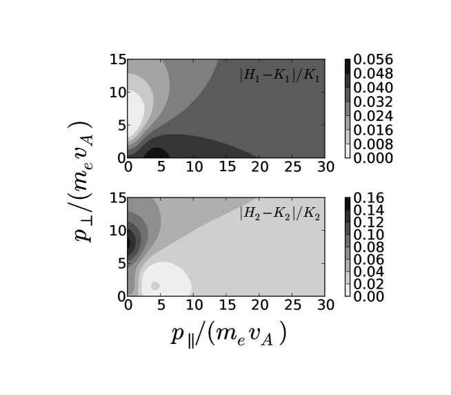
Figure 11: Difference between $H_{1}$ and $K_{1}$ (top panel) and $H_{2}$ and $K_{2}$ (bottom panel) in model solution B at $t=6.9\times 10^{7}\Omega^{-1}_{p}$.

Appendix C Fast-Wave Turbulence

In many situations involving turbulence, fluctuations or waves are excited at some large scale $\sim 1/k_{0}$ and then cascade to smaller scales. In our model, this large-scale excitation is represented by the term $S_{k}$ in Equation (5), where

$$\dot{E}_{0}=\frac{1}{2}\int d^{3}kS_{k},$$ (C1)

is the total energy injection rate. Since $S_{k}\propto e^{-k^{2}/k^{2}_{0}}$ in our model, wave injection is limited to small wavenumbers $\lesssim k_{0}$. If dissipation is only effective at wavenumbers exceeding some dissipation wavenumber $k_{d}$, then wavenumbers $\gg k_{0}$ and $\ll k_{d}$ are said to be in the inertial range of the turbulence. In steady state, the energy cascade rate in the inertial range must equal $\dot{E}_{0}$. From Equation (8), when waves reach a steady state in which $F_{k}=A_{1}g_{\theta}k^{-7/2}$, the energy cascade rate per solid angle per unit mass density is given by (Chandran, 2005),

$$\epsilon=\frac{9\pi^{2}c_{2}A_{1}^{2}g^{2}_{\theta}\sin^{2}\theta}{16v_{\rm A}},$$ (C2)

where $c_{2}\simeq 26.2$ is defined following Equation (53). The quantity $g_{\theta}$ is a function of $\theta$ that depends on the angular distribution of the input power at $k\lesssim k_{0}$. Equating the total energy injection rate with the total cascade power, we obtain

$$\dot{E}_{0}=2\pi\int_{0}^{\pi}\epsilon\sin\theta d\theta.$$ (C3)

If waves are injected isotropically (as in numerical calculation A4, B, C, and D, in which $\epsilon$ is independent of $\theta$), then $g_{\theta}=1/\sin\theta$ (Chandran, 2005), and

$$\dot{E}=\frac{9\pi^{3}c_{2}A_{1}^{2}}{4v_{\rm A}}\hskip 28.45274pt\mbox{(isotropic $\epsilon$)}.$$ (C4)

On the other hand, in our numerical calculations A1, A2, and A3, we take $S_{k}\propto\sin\theta$, which leads to $g_{\theta}=1$ (Chandran, 2005). Equation (C3) then yields

$$\dot{E}=\frac{3\pi^{3}c_{2}A^{2}_{1}}{2v_{\rm A}}\hskip 28.45274pt\mbox{(isotropic $F_{k}$)}.$$ (C5)

We can compare Equation (C5) to the cascade rate implied by the equation 3.3 in MLM96,

$$\dot{E}=\frac{14\pi^{2}A^{2}_{1}}{v_{\rm A}}.\hskip 28.45274pt\mbox{(MLM96)}$$ (C6)

The cascade rate in our model in Equation (C5) is larger than MLM96’s by a factor of $3\pi c_{2}/28=8.8$ for a fixed isotropic $F_{k}$. Therefore, if $\dot{E}$ is the same in our model and MLM96’s, then $F_{k}$ be will smaller in our model by a factor of $\simeq 3$.

References

- Aschwanden (2007) Aschwanden, M. J. 2007, ApJ, 661, 1242
- Benz (2008) Benz, A. O. 2008, Living Reviews in Solar Physics, 5, 1
- Brown (1971) Brown, J. C. 1971, Sol. Phys., 18, 489
- Carmichael (1964) Carmichael, H. 1964, NASA Special Publication, 50, 451
- Caspi & Lin (2010) Caspi, A., & Lin, R. P. 2010, ApJ, 725, L161
- Chandran (2003) Chandran, B. D. G. 2003, 599, 1426
- Chandran (2005) —. 2005, Physical Review Letters, 95, 265004
- Chandran (2008) —. 2008, Physical Review Letters, 101, 235004
- Cho & Lazarian (2002) Cho, J., & Lazarian, A. 2002, Physical Review Letters, 88, 245001
- Eichler (1979) Eichler, D. 1979, ApJ, 229, 413
- Ginzburg (1960) Ginzburg, V. L. 1960, The Propagation of Electromagnetic Waves in Plasmas (Oxford: Pergammon)
- Grigis & Benz (2004) Grigis, P. C., & Benz, A. O. 2004, A&A, 426, 1093
- Hirayama (1974) Hirayama, T. 1974, Sol. Phys., 34, 323
- Ishikawa et al. (2011) Ishikawa, S., Krucker, S., Takahashi, T., & Lin, R. P. 2011, ApJ, 737, 48
- Kennel & Engelmann (1966) Kennel, C., & Engelmann, F. 1966, Phys. Fluids, 9, 2377
- Kennel & Wong (1967) Kennel, C. F., & Wong, H. V. 1967, Journal of Plasma Physics, 1, 75
- Kopp & Holzer (1976) Kopp, R. A., & Holzer, T. E. 1976, Sol. Phys., 49, 43
- Krucker et al. (2010) Krucker, S., Hudson, H. S., Glesener, L., White, S. M., Masuda, S., Wuelser, J.-P., & Lin, R. P. 2010, ApJ, 714, 1108
- Krucker et al. (2011) Krucker, S., Hudson, H. S., Jeffrey, N. L. S., Battaglia, M., Kontar, E. P., Benz, A. O., Csillaghy, A., & Lin, R. P. 2011, ApJ, 739, 96
- Lin et al. (1981) Lin, R. P., Schwartz, R. A., Pelling, R. M., & Hurley, K. C. 1981, ApJ, 251, L109
- Lin et al. (2003) Lin, R. P., et al. 2003, ApJ, 595, L69
- Liu et al. (2009) Liu, W., Petrosian, V., & Mariska, J. T. 2009, ApJ, 702, 1553
- Lynn et al. (2012) Lynn, J. W., Parrish, I. J., Quataert, E., & Chandran, B. D. G. 2012, ArXiv e-prints
- Lynn et al. (2013) Lynn, J. W., Quataert, E., Chandran, B. D. G., & Parrish, I. J. 2013, ApJ, 777, 128
- Lynn et al. (2014) —. 2014, ArXiv e-prints
- Miller et al. (1996) Miller, J. A., Larosa, T. N., & Moore, R. L. 1996, ApJ, 461, 445
- Miller et al. (1997) Miller, J. A., et al. 1997, J. Geophys. Res., 102, 14631
- Petrosian et al. (2006) Petrosian, V., Yan, H., & Lazarian, A. 2006, ApJ, 644, 603
- Pongkitiwanichakul et al. (2012) Pongkitiwanichakul, P., Chandran, B. D. G., Karpen, J. T., & DeVore, C. R. 2012, ApJ, 757, 72
- Priest & Forbes (2000) Priest, E., & Forbes, T. 2000, Irish Astronomical Journal, 27, 235
- Rosenbluth et al. (1957) Rosenbluth, M. N., MacDonald, W. M., & Judd, D. L. 1957, Physical Review, 107, 1
- Schlickeiser & Miller (1998) Schlickeiser, R., & Miller, J. A. 1998, ApJ, 492, 352
- Selkowitz & Blackman (2004) Selkowitz, R., & Blackman, E. G. 2004, MNRAS, 354, 870
- Shalchi et al. (2004) Shalchi, A., Bieber, J. W., Matthaeus, W. H., & Qin, G. 2004, ApJ, 616, 617
- Shalchi & Schlickeiser (2004) Shalchi, A., & Schlickeiser, R. 2004, A&A, 420, 799
- Stix (1992) Stix, T. H. 1992, Waves in plasmas
- Tsuneta (1996) Tsuneta, S. 1996, ApJ, 456, 840
- Tsuneta et al. (1992) Tsuneta, S., Hara, H., Shimizu, T., Acton, L. W., Strong, K. T., Hudson, H. S., & Ogawara, Y. 1992, PASJ, 44, L63
- van de Vorst (2003) van de Vorst, H. 2003, Iterative Krylov Methods for Large Linear Systems (Cambridge: Cambridge Univ. Press)
- Yan & Lazarian (2004) Yan, H., & Lazarian, A. 2004, ApJ, 614, 757
- Yan & Lazarian (2008) —. 2008, ApJ, 673, 942
- Yan et al. (2008) Yan, H., Lazarian, A., & Petrosian, V. 2008, ApJ, 684, 1461
- Zakharov & Sagdeev (1970) Zakharov, V. E., & Sagdeev, R. Z. 1970, Sov. Phys. Dokl., 15, 439