Comfortability of a Team in Social Networks

Abstract

There are many indexes (measures or metrics) in Social Network Analysis (SNA), like density, cohesion, etc. We have defined a new SNA index called “comfortability ”. In this paper, core comfortable team of a social network is defined based on graph theoretic concepts and some of their structural properties are analyzed. Comfortability is one of the important attributes (characteristics) for a successful team work. So, it is necessary to find a comfortable and successful team in any given social network.

It is proved that forming core comfortable team in any network is NP-Complete using the concepts of domination in graph theory. Next, we give two polynomial-time approximation algorithms for finding such a core comfortable team in any given network with performance ratio $O(\ln\Delta)$, where $\Delta$ is the maximum degree of a given network (graph). The time complexity of the algorithm is proved to be $O(n^{3})$, where $n$ is the number of persons (vertices) in the network (graph). It is also proved that the algorithms give good results in scale-free networks.

1 Introduction

There are many factors, lack of which affect the group or team effectiveness. Team processes describe subtle aspects of interaction and patterns of organizing, that transform input into output. The team processes will be described in terms of seven characteristics: coordination, communication, cohesion, decision making, conflict management, social relationships and performance feedback. The readers are directed to refer Michan et al. [9] for further details of characteristics of team and Forsyth [3] for more details on group dynamics. In this paper, we discuss about an attribute or characteristic called “COMFORTABILITY ”, which is also essential for a successful team work. So, we defined it as a new SNA index in our paper [6].

Since the beginning of Social Network Analysis, Graph Theory has been a very important tool both to represent social structure and to calculate some indexes, which are useful to understand several aspects of the social context under analysis. Some of the existing indexes (measures or metrics) are betweenness, bridge, centrality, flow betweenness centrality, centralization, closeness, clustering coefficient, cohesion, degree, density, eigenvector centrality, path length. Readers are directed to refer Martino et. al. [8] for more details on indexes in SNA. In our paper [6], we defined a new SNA index called ‘comfortability ’. Based on this index, we have defined comfortable team, better comfortable team and highly comfortable team in our paper [6] and totally comfortable team in our paper [7].

Let the social network be represented in terms of a graph, with the vertex of the graph denotes a person (an actor) in the social network and an edge between two vertices in a graph represents relationship between two persons in the social network. All the networks are connected networks in this paper, unless otherwise specified. If the given network is disconnected, then each connected component of the network can be considered and hence it is enough to consider only connected networks. Hereafter, the word ‘team’ represents induced sub network (sub graph) of a given network (graph).

Following are some introduction for basic graph theoretic concepts. Some basic definitions from Slater et al. [4] are given below.

The graphs considered in this paper are finite, simple, connected and undirected, unless otherwise specified. For a graph $G$, let $V(G)$ (or simply $V$) and $E(G)$ denote its vertex (node) set and edge set respectively and $n$ and $m$ denote the cardinality of those sets respectively. The degree of a vertex $v$ in a graph $G$ is denoted by $deg_{G}(v)$. The maximum degree of the graph $G$ is denoted by $\Delta(G)$. The length of any shortest path between any two vertices $u$ and $v$ of a connected graph $G$ is called the distance between $u$ and $v$ and is denoted by $d_{G}(u,v)$. For a connected graph $G$, the eccentricity $e_{G}(v)=\max\{d_{G}(u,v):u\in V(G)\}$. If there is no confusion, we simply use the notions $deg(v)$, $d(u,v)$ and $e(v)$ to denote degree, distance and eccentricity respectively for the concerned graph. The minimum and maximum eccentricities are the radius and diameter of $G$, denoted by $r(G)$ and $diam(G)$ respectively. A vertex with eccentricity $r(G)$ is called a central vertex and a vertex with eccentricity $diam(G)$ is called a peripheral vertex.

For $v\in V(G)$, neighbors of $v$ are the vertices adjacent to $v$ in $G$. The neighborhood $N_{G}(v)$ of $v$ is the set of all neighbors of $v$ in $G$. It is also denoted by $N_{1}(v)$. $N_{j}(v)$ is the set of all vertices at distance $j$ from $v$ in $G$. A vertex $u$ is said to be an eccentric vertex of $v$, when $d(u,v)=e(v)$. If $A$ and $B$ are not necessarily disjoint sets of vertices, we define the distance from $A$ to $B$ as $dist(A,B)=\ min\{d(a,b):a\in A,b\in B\}$. Cardinality of a set $D$ represents the number of vertices in the set $D$. Cardinality of $D$ is denoted by $|D|$.

A vertex of degree one is called a pendant vertex. A walk of length $j$ is an alternating sequence $W:u_{0},e_{1},u_{1},e_{2},u_{2},\ldots,u_{j-1},e_{j},u_{j}$ of vertices and edges with $e_{i}=u_{i-1}u_{i}$. If all $j$ edges are distinct, then $W$ is called a trail. A walk with $j+1$ distinct vertices $u_{0},u_{1},\ldots,u_{j}$ is a path and if $u_{0}=u_{j}$ but $u_{1},u_{2},\ldots,u_{j}$ are distinct, then the trail is a cycle. A path of length $n$ is denoted by $P_{n}$ and a cycle of length $n$ is denoted by $C_{n}$. A graph $G$ is said to be connected if there is a path joining each pair of nodes. A component of a graph is a maximal connected sub graph. If a graph has only one component, then it is connected, otherwise it is disconnected. A tree is a connected graph with no cycles (acyclic).

We say that $H$ is a sub graph of a graph $G$, denoted by $H<G$, if $V(H)\subseteq V(G)$ and $uv\in E(H)$ implies $uv\in E(G)$ . If a sub graph $H$ satisfies the added property that for every pair $u,v$ of vertices, $uv\in E(H)$ if and only if $uv\in E(G)$, then $H$ is called an induced sub graph of $G$. The induced sub graph $H$ of $G$ with $S=V(H)$ is called the sub graph induced by $S$ and is denoted by $\left\langle S|G\right\rangle$ or simply $\left\langle S\right\rangle$.

Let $k$ be a positive integer. The $k^{th}$ power $G^{k}$ of a graph $G$ has $V(G^{k})=V(G)$ with $u,v$ adjacent in $G^{k}$ whenever $d(u,v)\leq k$.

The concept of domination was introduced by Ore [10] . A set $D\subseteq V(G)$ is called a dominating set if every vertex $v$ in $V$ is either an element of $D$ or is adjacent to an element of $D$. A dominating set $D$ is a minimal dominating set if $D-\{v\}$ is not a dominating set for any $v\in D$. The domination number $\gamma(G)$ of a graph $G$ equals the minimum cardinality of a dominating set in $G$.

A set $D$ of vertices in a connected graph $G$ is called a $k$-dominating set if every vertex in $V-D$ is within distance $k$ from some vertex of $D$. The concept of the $k$-dominating set was introduced by Chang and Nemhauser [1, 2] and could find applications for many situations and structures which give rise to graphs; see the books by Slater et al [4, 5]. So, dominating set is nothing but 1-dominating set.

Sampath Kumar and Walikar [11] defined a connected dominating set $D$ to be a dominating set $D$, whose induced sub-graph $\left\langle D\right\rangle$ is connected. The minimum cardinality of a connected dominating set is the connected domination number $\gamma_{c}(G)$.

The readers are also directed to refer Slater et al. [4] for further details of basic definitions, not given in this paper.

Let us recall the terminologies as follows: The symbol ($\rightarrow$) denotes “represents ”

• Graph $\rightarrow$ Social Network (connected)

• Vertex of a graph $\rightarrow$ Person in a social network

• Edge between two vertices of a graph $\rightarrow$ Relationship between two persons in a social network

• Induced subgraph of a graph $\rightarrow$ Team or Group of a social network.

Given a connected network of people. Our problem is to find a team (sub graph) which is less dispersive, highly flexible and performing better.

Note 1.

Notation 1:
In all the figures of this paper,

• $\{v_{1},v_{2},\ldots,v_{n}\}$ represent the vertex set of the graph $G$, that is,
  $V(G)=\{v_{1},v_{2},\ldots,v_{n}\}$.

• The numbers besides every vertex represents the eccentricity of that vertex. For example, in Figure 1, in the graph $G$, $e(v_{1})=5$, $e(v_{2})=4$, $e(v_{3})=3$, $e(v_{4})=3$, $e(v_{5})=4$ and $e(v_{6})=5$.

• The set notation $D=\{v_{1},v_{2},\ldots,v_{n}\}$ represents only the individual persons but does not represent the relationship between them.

• The notation $\left\langle D\right\rangle$ represents the team. $\left\langle D\right\rangle$ is the induced sub graph of $G$, which represents the persons as well as the relationship between them. So, the set $D$ represents only the team members and the team represents the persons with their relationship.

The remaining part of the paper is organized as follows:

• Section 2 discusses about prior work.

• Section 3 defines core comfortable team and analyses the concept with some examples.

• In section 4, an approximation algorithm is given for finding core comfortable team in any given network, with illustrations. Time complexity of the algorithm is analyzed. Also, correctness of the algorithm and performance ratio of the algorithm are proved in this section.

• In Section 5, another approximation algorithm is given, based on connected dominating set, for finding core comfortable team in any given network, with illustrations. Time complexity, correctness and performance ratio of this algorithm are discussed in this section.

• In section 6, some advantages of the two algorithms are given.

• Section 7 concludes the paper and discusses about some future work.

2 Prior Work

In our paper  [6], we defined characteristics of a good performing team and mathematically formulated them and given approximation algorithm for finding such a good performing team. In order to make this paper self-contained, we have given all the necessary definitions, examples and properties from our paper [6], which are needed for this paper, in this section.

Definition 1.

[6] A team is said to be good performing or successful if the team is

1. less dispersive

2. having good communication among the team members

3. easily accessible to the non- team members

4. a good service provider to the non-team members (for the whole network).

Mathematical Formulation
Domination $\rightarrow$ good service provider to the non-team members.
Connectedness $\rightarrow$ good communication among team members.

Definition 2.

Less Dispersive Set: [6] A set $D$ is said to be less dispersive, if $e_{\left\langle D\right\rangle}(v)<e_{G}(v)$, for every vertex $v\in D$.

Definition 3.

Less Dispersive Dominating Set: [6] A set $D$ is said to be a less dispersive dominating set if the set $D$ is dominating, connected and less dispersive. The cardinality of minimum less dispersive dominating set of $G$ is denoted by $\gamma_{comf}(G)$. A set of vertices is said to be a $\left\langle\gamma_{comf}-set\right\rangle$, if it is a less dispersive dominating set with cardinality $\gamma_{comf}(G)$.

Definition 4.

Comfortable Team: [6] A team $\left\langle D\right\rangle$ is said to be a comfortable team if $\left\langle D\right\rangle$ is less dispersive and dominating. Minimum comfortable team is a comfortable team with the condition: $|D|$ is minimum.

Example 1: Consider the graph (network) $G$ in Figure 1.

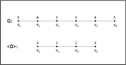
Figure 1: A Network and its Comfortable Team

Here, $G$ is a path of length six ($P_{6}$). $D=\{v_{2},v_{3},v_{4},v_{5}\}$. The induced sub graph $\left\langle D\right\rangle$ of $G$ forms a path of length four ($P_{4}$) and so it dominates all the vertices in $V-D$. Also, $\left\langle D\right\rangle$ forms the comfortable team of $G$, because
$e_{\left\langle D\right\rangle}(v_{2})=3<4=e_{G}(v_{2}).\ \Rightarrow e_{\left\langle D\right\rangle}(v_{2})<e_{G}(v_{2})$. Similarly, $e_{\left\langle D\right\rangle}(v_{i})<e_{G}(v_{i})$ for every $i=3,4,5$. Thus, $D$ forms less dispersive set and hence $\left\langle D\right\rangle$ forms the comfortable team of $G$. $\Rightarrow\gamma_{comf}(P_{6})=4$.

So, the problem is coined as: Find a team which is dominating, connected and less dispersive. It is to be noted that there are many graphs which do not have $\left\langle\gamma_{comf}-set\right\rangle$. So, we must try to avoid such kind of networks for successful team work.
Example 2: Consider the graph $G$ in Figure 2.

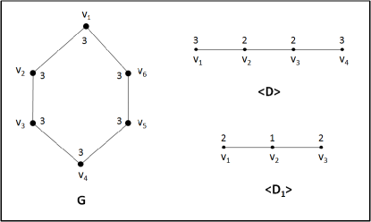
Figure 2: A Network and its CC Team

Here, $G$ is a cycle of length six ($C_{6}$). The vertices $v_{1}$ and $v_{4}$ dominate all the vertices of $G$. So, with connectedness, we can take $D=\{v_{1},v_{2},v_{3},v_{4}\}$. The set $D$ dominates $G$, but $D$ is not less dispersive, because,
$e_{\left\langle D\right\rangle}(v_{1})=3=e_{G}(v_{1})$ and $e_{\left\langle D\right\rangle}(v_{4})=3=e_{G}(v_{4})$. The vertices $v_{1}$ and $v_{4}$ maintained the original eccentricity as in $G$. Thus, $e_{\left\langle D\right\rangle}(v)<e_{G}(v)$, for every vertex $V\in D$ is not satisfied. So, $D$ is not less dispersive and hence $\left\langle D\right\rangle$ is not a comfortable team.
Also, $D_{1}=\{v_{1},v_{2},v_{3}\}$ forms less dispersive set in $G$, (from Figure 2), but $D_{1}$ is not dominating. The vertex $v_{5}$ is left undominated.

Note 2.

From the above discussion in Example 2, we get,

• the less dispersive set may not be dominating

• the dominating set may not be less dispersive.

So, under one of these two cases, the graph $G$ does not possess comfortable team. It is to be noted that not only $C_{6}$, but all the cycles $C_{n}$, do not possess a comfortable team. Also, there are infinite families of graphs which do not possess comfortable team.

Disadvantage of the comfortable team [6]:
As discussed in the Example 2, comfortable team does not exist in any given network. Infinite families of networks do not possess comfortable team.

The main aim of this paper is to find a team which is more comfortable and less dispersive, in any given social network.
So, we define a core comfortable team with a modification in the comfortable team in the next section.

3 Core Comfortable Team

As discussed in Note 2, the less dispersive set may not be dominating. So, we define less dispersive set with $k^{*}-$domination.

Definition 5.

Less Dispersive $k^{*}-$ Dominating Set:

A set $D$ is said to be a ‘less dispersive $k^{*}$-dominating’  set if $D$ is a less dispersive set and a $k^{*}-$ dominating set. That is,

1. $e_{\left\langle D\right\rangle}(v)<e_{G}(v)$, for every vertex $v\in D$ (less dispersive)

2. $dist(D,V-D)\leq k^{*}$ ($k^{*}-$ domination). This implies that $k^{*}\leq diam(G)$, (because any vertex in $V-D$ can reach $D$ at a distance of at most $diam(G)$).

Minimum cardinality of a ‘less dispersive $k^{*}$-dominating’  set of $G$ is denoted by $\gamma_{k^{*}comf}(G)$ and maximum cardinality of a ‘less dispersive $k^{*}$-dominating’  set of $G$ is denoted by $\Gamma_{k^{*}comf}(G)$.

Definition 6.

Core Comfortable Team: A team $\left\langle D\right\rangle$ is said to be a Core Comfortable (CC) team if $\left\langle D\right\rangle$ is less dispersive $k^{*}$-dominating.

• Min CC team is a CC team with the condition: $|D|$ and $k^{*}$ are minimum

• Max CC team is a CC team with the condition: $|D|$ is maximum and $k^{*}$ is minimum.

Example 3: Consider the graph $G$ ($C_{6}$) in Figure 2. In $C_{6}$, $D_{1}=\{v_{1},v_{2},v_{3}\}$ forms a less dispersive 2-dominating set, because

1. $e_{\left\langle D_{1}\right\rangle}(v_{i})<e_{G}(v_{i})$, for $i=1,2,3$.

2. $k^{*}=2$, because $v_{5}$ is reachable from $D_{1}$ by distance two, $v_{4}$ and $v_{6}$ are reachable from $D_{1}$ by distance one. $\Rightarrow dist(D_{1},V-D_{1})\leq 2$.

Thus, CC team exists in $C_{6}$ and hence $\gamma_{2comf}(G)=\Gamma_{2comf}(G)=3$.

Theorem 1.

Forming core comfortable team in a given network is NP-complete.

Proof.

Let $D$ be a minimum less dispersive $k^{*}-$ dominating set of $G$.
$\Rightarrow D$ is a connected $k^{*}-$ dominating set of $G$ (since any less dispersive set is a connected set).
$\Rightarrow D$ is a connected dominating set of $G^{k^{*}}$ (by definition of the graph $G^{k}$).
Finding $\gamma_{c}(G)$, for any graph $G$ is NP-complete (by Slater et al. [4]).
$\Rightarrow$ Finding $\gamma_{c}(G^{k^{*}})$ is NP-complete.
$\Rightarrow$ Finding minimum less dispersive $k^{*}-$ dominating set of $G$ is NP-complete (by above points).
Thus forming core comfortable team in a given network is NP-complete. ∎

Next, we give two polynomial time approximation algorithms for finding core comfortable team in any given network.

4 Approximation Algorithm 1

In this section, we give a polynomial-time approximation algorithm for finding CC team from a given network.

4.1 Notation 2

• $D\rightarrow$ minimum less dispersive, $k^{*}$-dominating set.

• $D_{1}\rightarrow$ minimal less dispersive, $k$-dominating set, (output of our algorithm). $\Rightarrow|D_{1}|\geq|D|$.

• $k^{*}\rightarrow$ the distance between two sets $D$ and $V-D$, that is,
  $dist(D,V-D)\leq k^{*}$.

• $k\rightarrow$ the distance between two sets $D_{1}$ and $V-D_{1}$, that is,
  $dist(D_{1},V-D_{1})\leq k$.

• Instant $D\rightarrow$ The set $D$ at a particular iteration.

• Performance ratio = $\displaystyle\frac{|minimal\ set|}{|minimum\ set|}$.

4.2 Algorithm GOCOM

A polynomial time approximation algorithm for finding CC team is given below.
Input: $G$.
Output: $D_{1}$, which is a less dispersive, $k$-dominating set, so that $\left\langle D_{1}\right\rangle$ is a core comfortable team.
GOCOM(G)

1. Choose a central vertex $v$ (ties can be broken arbitrarily) and add it to $D_{1}$.

2. If $diam(G)$ is even, then choose all the vertices in $N_{j}(v)$, for $j\leq\displaystyle\frac{diam(G)}{2}$ and add them to $D_{1}$.
   else choose all the vertices in $N_{j}(v)$, for $j\leq\displaystyle\frac{(diam(G)-1)}{2}$ and add them to $D_{1}$.

3. Put $i=\left\lfloor\displaystyle\frac{diam(G)}{2}\right\rfloor$.

4. If $e_{\left\langle D_{1}\right\rangle}(v)<e_{G}(v)$, for every vertex $v\in D_{1}$, then Goto next step (step 5), else Goto Step 7.

5. Put $i=i+1$.

6. Choose all vertices from $N_{i}(v)$ and add it to $D_{1}$. Then GOTO step 4.

7. Remove suitably some vertices from $D_{1}$ (say from $D_{1}\cap N_{i-1}(v)$, from $D_{1}\cap N_{i-2}(v)$, and so on) such that the condition in step 4 is satisfied.

8. Print $D_{1}$.

9. Stop.

Note 3.

At each iteration after forming $D_{1}$, we check up the condition:

$$e_{\left\langle D_{1}\right\rangle}(v)<e_{G}(v),\ for\ every\ vertex\ v\in D_{1}.$$ (1)

If the condition 1 is not satisfied in Step 4, then the Step 7 is executed in the algorithm. We remove some vertices from $D_{1}$ until the condition 1 is satisfied.

If the condition 1 is satisfied, then we add some vertices to $D_{1}$. There may be a question: why should the process be continued? We add some vertices to $D_{1}$, in order to minimize $k$. Our aim is to minimize $k$ as well as to satisfy the condition 1.

So, in Step 6, we add some vertices to $D_{1}$ and check up the condition 1.

If the condition 1 is satisifed, then we proceed to add vertices to $D_{1}$. But, we can not go on adding vertices to $D_{1}$, because at one stage, the condition  1 will not be satisfied. Then the step 7 will be executed.

After Step 7 is executed, the condition  1 is satisfied. So, no further addition and deletion of vertices are done. The algorithm prints $D_{1}$ and ends.

Note 4.

The algorithm GOCOM finds a CC team. If Min CC team is needed, some vertices can be removed from the output set such that $k^{*}$ is minimum. If Max CC team is needed, then some vertices could be added to the output such that condition 1 is satisified and $k^{*}$ is minimum.

4.3 Illustration

Consider the network (graph) $G$ as in the Figure 3. In this network, $diam(G)=5$.

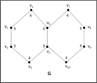
Figure 3: Illustration Figure

Inititally, let us choose the central vertex $v_{6}$ and add them to $D_{1}$. As $diam(G)$ is odd, let us choose up to $\frac{diam(G)-1}{2}=2$ neighborhoods of $v_{6}$ and add them to $D_{1}$. Now, instant $D_{1}=\{v_{1},v_{2},v_{4},v_{5},v_{6},v_{7},v_{8},v_{10}\}$. But, we can see in Figure 4 that vertices $v_{4},v_{5}$ and $v_{10}$ of $D_{1}$ at an intermediate interation violate the condition 1. In order to make $D_{1}$ maintain the condition 1, we remove some vertices from $D_{1}$.

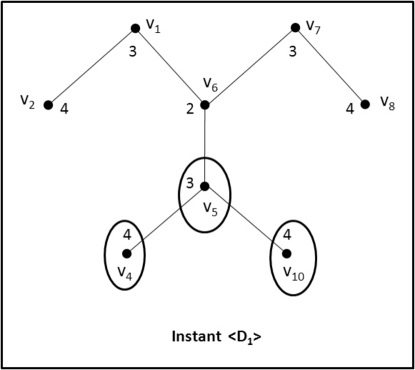
Figure 4: Intermediate Iteration showing vertices violating the condition (1)

We can either remove those vertices $v_{4},v_{5}$ and $v_{10}$ or the vertices $v_{2}$ and $v_{8}$, so that the condition 1 is satisfied. So, we get two different outputs. Let us make the first one as $D_{1}=\{v_{1},v_{2},v_{6},v_{7},v_{8}\}$ and the other one as $D_{2}=\{v_{1},v_{4},v_{5},v_{6},v_{7},v_{10}\}$. Refer Figure 5. Both outputs satisfy the condition 1 and hence both $\left\langle D_{1}\right\rangle$ and $\left\langle D_{2}\right\rangle$ are core comfortable teams. But, for$D_{1}$, we get $k=2$ and for $D_{2}$, we get $k=1$.

$D_{1}$ is a maximal CC team for $k=2$ and hence $\Gamma_{2comf}(G)=5$. Also, for $k=2$, we see that $D_{3}=\{v_{5},v_{6}\}$ forms a minimal CC team. The vertices $v_{5}$ and $v_{6}$ are suuficient and every vertex in $V-D_{3}$ is reachable from $D_{3}$ by a distance of at most two. Also, $D_{3}$ satisfies the condition 1. Refer Figure 5. Thus, $D_{3}$ is a minimal CC team and hence $\gamma_{2comf}(G)=2$.

For $k=1$, $D_{2}$ is a minimal as well as a maximal CC team and hence $\gamma_{1comf}(G)=\Gamma_{1comf}(G)=6$.

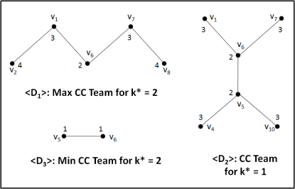
Figure 5: Three Different Outputs

Note 5.

From the Illustration 4.3, we can observe that the core comfortable team is not unique for a given network. A social network may have many core comfortable teams. We can choose one team among all the teams whichever is suitable for a particular situation. We can choose any CC team (minimum or maximum) according to our need for a particular situation.

4.4 Time Complexity of the Algorithm GOCOM

Let us discuss the time complexity of the algorithm as follows:

The definition of CC team and the algorithm GOCOM is dependent on eccentricity of every vertex. So, we have to find eccentricity of every vertex of $G$. By Performing Breadth-First Search (BFS) method from each vertex, one can determine the distance from each vertex to every other vertex. The worst case time complexity of BFS method for one vertex is $O(n^{2})$. As the BFS is method is done for each vertex of $G$, the resulting algorithm has worst case time complexity $O(n^{3})$. As eccentricity of a vertex $v$ is defined as $e(v)=\max\{d(u,v):u\in V(G)\}$, finding eccentricity of vertices of $G$ takes at most $O(n^{3})$.

Thus, the total worst case time complexity of the algorithm is at most $O(n^{3})$.

4.5 Correctness of the Algorithm GOCOM

In order to prove that the algorithm GOCOM yields a CC team, it is sufficient to prove that the condition in Step 4 of the algorithm is satisfied. As proof follows from Note 3, we state the following theorem without proof.

Theorem 2.

$e_{\left\langle D_{1}\right\rangle}(v)<e_{G}(v)$, for every vertex $v\in D_{1}$, where $D_{1}$ is the output of our Algorithm GOCOM.

4.6 Performance Ratio of the Algorithm GOCOM

It is to be noted that the algorithm has two parameters, namely, $|D|$ and $k^{*}$. The set $D$ represents the team members of CC team, and $k^{*}$ represents the distance between the team members and non-team members. We find performance ratio of the algorithm for finding Min CC team. So, it is necessary that both $D$ and $k^{*}$ should be minimized simultaneously.

The following theorem gives the performance ratio for finding the minimum less dispersive $k^{*}-$ dominating set. Performance ratio of the algorithm for finding the minimum CC team is equal to $|D_{1}|/|D|$.

Theorem 3.

The performance ratio of the algorithm for finding Min CC team is at most $O(\ln\Delta(G))$.

Proof.

Let $D_{1}$ be a minimal less dispersive $k-$ dominating set of $G$ and
let $D$ be a minimum less dispersive $k^{*}-$ dominating set of $G$.
$\Rightarrow D$ is a connected $k^{*}-$ dominating set of $G$ (since any less dispersive set is a connected set).
$\Rightarrow D$ is a connected dominating set of $G^{k^{*}}$ (by definition of the graph $G^{k^{*}}$).
Performance ratio for finding $\gamma_{c}(G)$ is at most $O(\ln\Delta(G))$.
$\Rightarrow$ Performance ratio for finding $\gamma_{c}(G^{k^{*}})$ is at most $O(\ln\Delta(G^{k^{*}}))$.
But, $\Delta(G^{k^{*}})\leq(\Delta(G))^{k^{*}}$.
$\Rightarrow$ Performance ratio for finding $\gamma_{c}(G^{k^{*}})$ is at most $O(\ln(\Delta(G))^{k^{*}})=O(k^{*}\ln\Delta(G))=O(\ln\Delta(G))$.
Thus, the performance ratio of the algorithm for finding Min CC team is at most $O(\ln\Delta(G))$. ∎

Next, let us give the performance ratio for finding $k^{*}$. Performance ratio of the algorithm for finding $k^{*}$ is equal to $k/k^{*}$.

Theorem 4.

The performance ratio of the Algorithm GOCOM for finding $k^{*}$ is at most $r(G)$.

Proof.

Let us recall from Notation 2: $dist(D,V-D)\leq k^{*}$ and $dist(D_{1},V-D_{1})\leq k$, that is, $k$ and $k^{*}$ denote the minimal parameter and the minimum parameter respectively.

In the Algorithm GOCOM, we start from a central vertex. So, the output set $D_{1}$ always contains at least one central vertex. This implies that any vertex in $V-D_{1}$ is reachable from $D_{1}$ by distance at most $r(G)$. Thus, $k\leq r(G)$.

Also, as 1-dominating set is possible in many cases, $k^{*}\geq 1$.
Thus, $\frac{k}{k^{*}}\leq r(G)$. ∎

5 Approximation Algorithm 2

In this section, we give another approximation algorithm for finding core comfortable team and analyze its time complexity, correctness and performance ratio.
Algorithm CONCOMF:
Input: $G$.
Output: $D_{1}$, which is a less dispersive $k-$ dominating set, so that $\left\langle D_{1}\right\rangle$ is a CC team.
CONCOMF($G$)

1. Find a connected $k-$ dominating set of $G$ (using an approximation algorithm).

2. Store all the vertices in $D_{1}$.

3. If $e_{\left\langle D_{1}\right\rangle}(v)<e_{G}(v)$, for every vertex $v\in D_{1}$, then GOTO Step 5 else Goto Step 4 (next step).

4. Remove suitably some vertices from $D_{1}$ such that the condition in step 3 is satisfied .

5. Print $D_{1}$.

6. Stop.

Note 6.

The algorithm CONCOMF finds a CC team. If Min CC team is needed, in Step 1, find a minimal $k-$ dominating set of $G$. If Max CC team is needed, in Step 1, find a maximal connected $k-$ dominating set of $G$. Executing the Algorithm CONCOMF in graph $G$ of Figure 3, we get $D_{1}$ is maximal CC team and $D_{3}$ is minimal CC team for $k=2$ and $D_{2}$ is a minimal and maximal CC team for $k=1$.

5.1 Time Complexity of the Algorithm CONCOMF

The worst case time complexity of the approximation algorithm for finding connected dominating set is at most $O(n^{3})$. Also, as discussed in the Section 4.4, the definition of CC team is dependent on eccentricity of every vertex and finding eccentricity of vertices of $G$ takes at most $O(n^{3})$ in worst case.

Thus, the total worst case time complexity of the algorithm is at most $O(n^{3})$.

5.2 Correctness of the Algorithm CONCOMF

At the end of Step 4 in Algorithm CONCOMF, the output $D_{1}$ satisfies the condition 1. So, we state the following theorem without proof.

Theorem 5.

$e_{\left\langle D_{1}\right\rangle}(v)<e_{G}(v)$, for every vertex $v\in D_{1}$, where $D_{1}$ is the output of our Algorithm GOCOM.

5.3 Performance Ratio Of the Algorithm CONCOMF

As discussed in the Section 4.6, for finding a Min CC team, it is necessary that the two parameters $|D|$ and $k^{*}$ should be minimized simultaneously.

The following theorem gives the performance ratio for finding the minimum less dispersive $k^{*}-$ dominating set. As proof follows form Theorem 3, we state the following theorem without proof.

Theorem 6.

The performance ratio of the Algorithm CONCOMF for finding Min CC team is at most $O(\ln\Delta(G))$.

Next, we give performance ratio of the algorithm CONCOMF for finding $k^{*}$.

Theorem 7.

The performance ratio of the Algorithm CONCOMF for finding $k^{*}$ is at most $diam(G)$.

Proof.

As 1-dominating set is possible in many cases, $k^{*}\geq 1$.

Also, any vertex in $D_{1}$ is reachable form $V-D_{1}$ by a distance of at most $diam(G)$. This implies that $k\leq diam(G)$.

Thus, $\frac{k}{k^{*}}\leq diam(G)$. ∎

6 Advantages

Advantage 1: The algorithms give good results in scale free networks for finding core comfortable team.
Explanation: The performance ratio of the Algorithms GOCOM and CONCOMF for finding $k^{*}$, are dependent on $r(G)$ and $diam(G)$ respectively (by Theorems 7 and  4). It is known that the growing scale-free networks have almost constant diameter in practice. So, the algorithms give constant performance ratio in scale free networks.
Advantage 2: The algorithms can be applied in any random networks for finding CC team.
Explanation: From the theorems 3, 4, 6 and 7, it is clear that the performance ratio of the algorithm for finding $|D|$ and $k^{*}$ is dependent on $diam(G)$ and $\Delta(G)$. As both these terms can be expressed in terms of the probability $p$, the performance ratio of the algorithm can be easily obtained for random networks in terms of $p$.
Advantage 3: CC team can be obtained in disconnected networks also using the algorithms.
Explanation: If the network (graph) is disconnected, then as mentioned in the Section 1, algorithm can can be applied to each connected component of the network. Thus, algorithm can be applied to find CC team in any given network.

7 Conclusion

In this paper, core comfortable team of a social network is defined. It is proved that forming core comfortable team in any given network is NP-complete. Two polynomial time approximation algorithms are given for finding a CC team in any given network and the time complexity of those algorithms are given to be $O(n^{3})$, where $n$ is the number of vertices of $G$. The correctness of the algorithms are analyzed. The performance ratio of the algorithms for finding Min CC team is proved to be $O(\ln\Delta)$, where $\Delta$ is the maximum degree of $G$. The performance ratio of the two algorithms for finding $k^{*}$ is proved to be at most $r(G)$ and $diam(G)$ respectively. It is also proved that the algorithms give good results in scale free networks.

7.1 Future Work

The algorithms can be applied in a particular social network, for example, Poisson network and can be tried to reduce the performance ratio in that network. Algorithms can be implemented to get exact values also in some particular networks, for example scale free networks and so on. Also, as discussed in Note 5, a social network can have many CC teams. So, we can analyse the different situations for which the CC teams are suitable.

References

- [1] G.J. Chang, k-domination and graph covering problems, Ph.D. Thesis, School of OR and IE, Cornell University, Ithaca, NY, 1982.
- [2] G.J. Chang, G.L. Nemhauser, The k-domination and k-stability problems on sun-free chordal graphs, SIAM J. Algebraic Discrete Methods, 5, (1984), 332-345.
- [3] Donelson R.Forsyth, Group Dynamics, 3rd ed. Belmont, CA: Wadsworth, (1999).
- [4] T. W. Haynes, S. T. Hedetniemi, P. J. Slater, Fundamentals of domination in graphs, Marcel Dekker, New York, (1998).
- [5] T.W.Haynes, Stephen T.Hedetniemi, Peter J.Slater, Domination in Graphs: Advanced Topics, Marcel Dekker, Inc. New York, (1998).
- [6] Lakshmi Prabha S, T.N.Janakiraman, Polynomial-time Approximation Algorithm for finding Highly Comfortable Team in any given Social Network, ArXiv, 18 May 2014, http://arxiv.org/abs/1405.4534 or http://arxiv.org/pdf/1405.4534v1.pdf.
- [7] Lakshmi Prabha S, T.N.Janakiraman, Polynomial-time Approximation Algorithm for finding Totally Comfortable Team in any given Social Network, Accepted in Proceddings of the ICHSS 2014.
- [8] F.Martino and A.Spoto, Social Network Analysis: A brief theoretical review and further perspectives in the study of Information Technology, PsychNology Journal, Volume 4, Number 1, (2006), pp. 53-86.
- [9] S. Mickan and S.Rodger, Characteristics of effective teams: a literature review, Australian Health Review, Vol 23 No 3, (2000), 201-208.
- [10] O.Ore, Theory of Graphs, Amer. Soc. Colloq. Publ. vol. 38. Amer. Math. Soc., Providence, RI, (1962).
- [11] E. Sampathkumar, H. B. Walikar, The connected domination number of a graph, J.Math.Phys.Sci., 13, (1979), 607-613.