ABSTRACT. Does quantum mechanics matter at everyday scales? We generally assume that its consequences are confined to microscopic scales. It would be very surprising if quantum effects were to be manifest in a macroscopic system. This has been claimed for the problem of balancing a pencil on its tip. The claim has also been disputed. We argue that the behaviour of a tipping pencil can be explained by the asymptotic properties of the complete elliptic function, and can be understood in purely classical terms.

Modelling a balanced pencil

We have all tried to balance a pencil on its sharp end. Although this is essentially impossible, you may often notice someone at a tedious committee meeting trying to do it. We examine the dynamics and see why this unstable equilibrium is unattainable. We can analyse the pencil using rigid body dynamics, but it is simpler to replace it by a point mass constrained by a light rod to move in a circle centred at the point of contact with the underlying surface.

We model the pencil as an inverted simple pendulum with a bob of mass $m$ at one end of a rigid massless rod of length $\ell$, the other end being fixed at a point. The position of the bob corresponds to the centre of oscillation of the pencil. We ignore the fine structural details of the pencil tip, treating it as a point.

For equilibrium, the bob must be positioned exactly over the fixed point, and the angular momentum must vanish. In classical physics, this is theoretically possible. In a quantum system, it is precluded by the uncertainty principle.

Dynamics of a simple pendulum

The story of how Galileo found inspiration in the Cathedral at Pisa is well known. His mind must have wandered from his prayers as he noticed the regular oscillations of the chandelier. He concluded, using his pulse to measure the time, that the period of the back-and-forth swing was constant. Had he been able to measure it more precisely, he would have realised that the swing-time increases with the amplitude.

Denoting the deflection of the pendulum from the downward vertical by $\theta$, the dynamical equation is

$$m\ell\ddot{\theta}=-mg\sin\theta$$

where $m$ is the mass of the bob, $\ell$ is the length of the rod and $g$ is the acceleration due to gravity. Defining the frequency $\omega=\sqrt{g/\ell}$, this is

$$\ddot{\theta}+\omega^{2}\sin\theta=0\,.$$

For small amplitude motion, we can replace the sine by its argument and the solution is simple harmonic motion with period $T=2\pi/\omega$, independent of the amplitude.

For finite — that is, non-infinitesimal — motions, the equation is harder to solve but it is a standard problem in classical dynamics. The solution may be expressed as

$$\sin\textstyle{\frac{1}{2}}\theta=\sin\textstyle{\frac{1}{2}}\theta_{0}\ \mathrm{sn}[\omega(t-t_{0}),k]$$

where $\theta_{0}$ is the amplitude, $k=\sin\textstyle{\frac{1}{2}}\theta_{0}$ and $\mathrm{sn}$ is the Jacobian elliptic function (see Synge and Griffith, 1959 for full details). The period is

$$T=\frac{4K}{\omega}$$

where $K=K(k)$ is the complete elliptic integral of the first kind,

$$K(k)=\int_{0}^{\pi/2}\frac{\mathrm{d}\phi}{\sqrt{1-k^{2}\sin\phi}}\,.$$

For small amplitude — and therefore small $k$ — $K$ is approximately $\pi/2$, so $T\approx{2\pi}/{\omega}$, as in the linear case. The function $K$ varies very slowly with $k$ so that, for moderate amplitudes, the period depends only weakly on the value of $\theta_{0}$. However, $K$ is unbounded as $\theta_{0}\rightarrow\pi$ and the period becomes infinitely long in this limit (see Fig. 1).

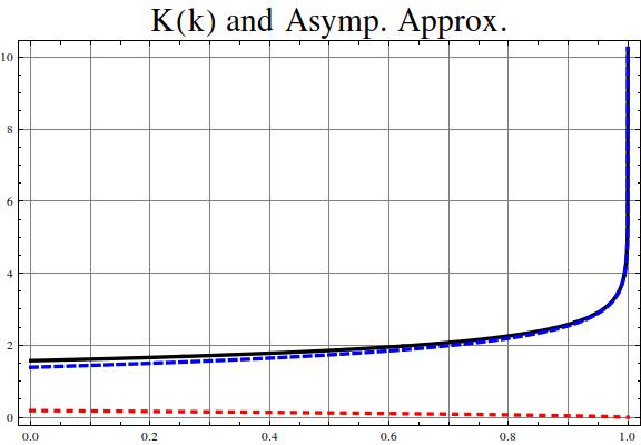
Figure 1: Complete elliptic integral of the first kind for $0<k^{2}<1-10^{-8}$. Solid: $K(k)$. Dashed: $\log(4/k^{\prime})$. Dotted: Difference, $K(k)-\log(4/k^{\prime})$.

Asymptotic Estimate of the Period

There is a solution $\theta\equiv\pi$, independent of time, where the pendulum remains stationary in an inverted position. This corresponds to a pencil balanced perfectly on its tip with its centre of mass exactly above the contact point. However, this solution is unstable and the slightest disturbance will cause the bob to move away from equilibrium.

The equilibrium implies initial conditions $\theta(0)=\theta_{0}=\pi$ and $\dot{\theta}(0)=\omega_{0}=0$. From the viewpoint of quantum mechanics, we are not free to specify both the angle $\theta_{0}$ and angular momentum $p_{0}=m\ell^{2}\omega_{0}$ exactly, since they are complementary variables, subject to the Heisenberg uncertainty principle:

$$\Delta\theta_{0}\cdot\Delta p_{0}\geq\textstyle{\frac{1}{2}}\hbar\,.$$

In the classical case there is no such limitation. However, we will choose initial conditions such that the deviation of the pendulum from its unstable equilibrium is at the quantum scale.

We set the pendulum parameters to $m=0.1\,$kg and $\ell=0.1\,$m. Assuming that at $t=0$ the bob is stationary ($p_{0}=0$) and its displacement from the vertical is at the atomic scale, we set

$$\theta_{0}=\pi-\delta\qquad\mbox{where}\qquad\delta=10^{-10}\,\mbox{rad}\,,$$

and compute the quarter-period using the classical formula $T/4=K/\omega$. The linear displacement of the bob is $\ell\delta=10^{-11}\,$m, less than an atomic radius.

With $g=10\,$m s^-2 we have $\omega=\sqrt{g/\ell}=10\,$s^-1 and

$$k=\sin\textstyle{\frac{1}{2}}\theta_{0}=\sin\left(\displaystyle{\frac{\pi}{2}-\frac{\delta}{2}}\right)=\cos\left(\displaystyle{\frac{\delta}{2}}\right)\approx 1-\displaystyle{\frac{1}{8}\delta^{2}}$$

We define $k^{\prime}$ by $k^{2}+k^{\prime 2}=1$. Then

$$k^{2}\approx 1-\displaystyle{\frac{1}{4}\delta^{2}}\qquad\mbox{implies}\qquad k^{\prime}\approx\displaystyle{\frac{\delta}{2}}$$

We can use an asympototic expression for the integral $K(k)$. The Digital Library of Mathematical Functions gives the expansion

$$K(k)=\sum_{m=0}^{\infty}\left[\frac{(\textstyle{\frac{1}{2}})_{m}}{m!}\right]^{2}k^{\prime 2m}\left(\log\left(\frac{1}{k^{\prime}}\right)+d(m)\right)$$

(DLMF, Eqn. 19.12.1. See this reference for full notation). This expansion is valid for $0<|k|<1$. For $k\approx 1$ we can consider only the first term:

$$K(k)\approx\left(\log\left(\frac{1}{k^{\prime}}\right)+2\log 2\right)=\log\left(\frac{4}{k^{\prime}}\right)\,.$$

But since $k^{\prime}\approx\textstyle{\frac{1}{2}}\delta$, this means

$$K(k)\approx\log\left(\frac{4}{k^{\prime}}\right)=\log\left(\displaystyle{\frac{8}{\delta}}\right)\,.$$

Using the numerical value $\delta=10^{-10}$, we get $K=25.1$. Finally, since $\omega=10\,$s^-1, the quarter-period is

$$\frac{T}{4}=\frac{K}{\omega}=2.51\,\mbox{seconds}.$$

The conclusion is that, even with a tiny deviation of the initial position from vertical — less than the width of an atom — the bob will reach the bottom point within just a few seconds.

Solution in Elementary Functions

We can get an estimate of the time-scale for motion starting near the unstable equilibrium without using elliptic integrals (Morin, 2008). If $\psi$ is the angle between the rod and the upward vertical, then the motion is governed by

$$m\ell\ddot{\psi}=mg\sin\psi\,.$$

Defining the time scale $\tau=\sqrt{\ell/g}$, the motion near equilibrium, where $\psi$ is small, is described by

$$\ddot{\psi}-\left(\frac{1}{\tau^{2}}\right)\psi=0$$

and the solution is

$$\psi(t)=\textstyle{\frac{1}{2}}[\psi_{0}+\tau v_{0}]\exp\left({t}/{\tau}\right)+\textstyle{\frac{1}{2}}[\psi_{0}-\tau v_{0}]\exp\left(-{t}/{\tau}\right)$$

where $\psi_{0}=\psi(0)$ and $v_{0}=\dot{\psi}(0)$. If $\psi_{0}=v_{0}=0$, we get the (unstable) stationary solution $\psi\equiv 0$. The negative exponential term is of significance only if the coefficient of the growing term vanishes. Since we are interested in the growing solution, we drop this second term.

The initial conditions are constrained by the uncertainty principle

$$\Delta_{x}\Delta_{p}=(\ell\psi_{0})\times(m\ell v_{0})\geq\textstyle{\frac{1}{2}}\hbar\,.$$

We assume that the uncertainties in the dimensionless quantities $\pi-\theta_{0}$ and $\omega_{0}/\omega$ are comparable in magnitude. This is an arbitrary but reasonable choice, and the results are not sensitively dependent on it. The coefficient $\textstyle{\frac{1}{2}}(\psi_{0}+\tau v_{0})$ is minimum when the two components are equal. Thus, we set

$$\psi_{0}=\sqrt{\frac{\tau\hbar}{2m\ell^{2}}}\quad\qquad\mbox{and}\quad\qquad v_{0}=\sqrt{\frac{\hbar}{2m\ell^{2}\tau}}$$

Then the solution becomes

$$\sqrt{\frac{\tau\hbar}{2m\ell^{2}}}\exp\left(\frac{t}{\tau}\right)$$

Since we wish to know how quickly this grows, let us set it equal to unity. Substituting numerical values $\ell=10^{-1}\,$m and $g=10\,$m s^-2, we have $\tau=10^{-1}$s, so that

$$t=-\frac{\tau}{2}\log\left(\frac{\tau\hbar}{2m\ell^{2}}\right)=-\frac{1}{20}\log\left(\frac{10^{-34}}{2\times 10^{-2}}\right)=3.72\,\mbox{s}\,.$$

Once again, we find that, even with the smallest disturbances that quantum physics will allow, the time for the pendulum to swing to the bottom is less than four seconds.

Discussion

Are the above results really due to quantum effects? It seems not: in a classical system, there are no constraints on the initial conditions. There is an equilibrium solution, corresponding to a perfectly balanced pencil. It is effectively unattainable, but theoretically possible. In reality, there are always small errors in setting the initial conditions. What the analysis of the inverted pendulum shows is that, however tiny the initial displacement, the pencil will drop within a few seconds. This is a consequence of the asymptotic properties of the complete elliptic function. Persistence of balance is impossible in practice.

Morin (2008) interprets the tipping pencil as a macroscopic manifestation of quantum mechanics. He concludes that ‘It is remarkable that a quantum effect on a macroscopic object can produce an everyday value for a time scale.’ However, Easton (2007) concludes that quantum effects are not responsible for the observed behaviour of pencils, describing this idea as ‘an urban myth of physics’.

Conclusion

The above analysis of a balanced pencil can be carried through purely in the context of classical mechanics, without any reference to the uncertainty principle. In that context, we are free to choose arbitrary initial conditions. The time to tip is just a few seconds, even when the deviation of the initial state from the ideal vertical or equilibrium position is of the order of an atomic radius. This is a consequence of the asymptotic behaviour of the elliptic integral, which tends logarithmically to infinity as $k\rightarrow 1$. The tipping is not a quantum effect, but the result is certainly surprising.

Sources

$\bullet$ DLMF: NIST Digital Library of Mathematical Functions. Release 1.0.8 of 2014-04-25. http://dlmf.nist.gov/19.12.E1.

$\bullet$ Easton, Don, 2007: The quantum mechanical tipping pencil — a caution for physics teachers. Eur. J. Phys., 28, 1097–1104.

$\bullet$ Morin, David, 2008: Introduction to Classical Mechanics: With Problems and Solutions, Cambridge University Press. ISBN: 978-0521876223

$\bullet$ Synge, J. L. and B. A. Griffith, 1959: Principles of Mechanics. McGraw-Hill, Third Edition, 552pp.

[Correspondence to Peter.Lynch :at: ucd.ie]