Velocities hasten to tell us about the Universe

Abstract

The peculiar velocities of galaxies are driven by gravity, and hence hold the promise of probing details of how gravity forms structures. In particular it is possible to constrain cosmological parameters and to test extensions to the standard model, such as modifications to the theory of gravity or the existence of primordial density perturbations which are non-Gaussian. This constraining power has been frustrated by systematic effects, but we appear to be entering an era when velocity measurements may finally be living up to their promise.

1 Introduction

Gravity grows galaxies from low contrast seed perturbations, and hence the galaxies will have motions which depend on the neighbouring density field. It has been understood since at least the 1960s (e.g. in the work of van Albada) that so-called “peculiar velocities” could help us to understand structure formation. In the 1970s the theoretical framework for such calculations was worked out (by Peebles and others) and by the 1980s there was a vigorous programme of estimating velocities and using them to constrain cosmologies.

The cosmic velocity field appeared to yield a high average density for the Universe and hence provided support for the “Standard Cold Dark Matter” paradigm (e.g., , 1993). However, it became clear that the determination of redshift-independent distances (necessary to estimate the velocities) was fraught with problems, leading to correlated errors that were fiendishly difficult to get rid of. Hence, by the 1990s, the use of velocities was largely abandoned in favour of other cosmological probes.

However, the situation now seems to be changing for the better, with new data sets and techniques enabling the cosmic flow field to be mined for cosmological information. This is a gratifying development, since velocities offer some distinct advantages as tests of the cosmological paradigm in which gravity plays a dominant role on large scales.

2 Testing the standard model

In the Universe, galaxies are not only moving outwards with cosmic expansion (known as the Hubble flow), but also have their own peculiar motions, coming from initial perturbations enhanced by gravity. The observed galaxy redshift is the combined effect of cosmic expansion and the radial component of these peculiar velocities (, 1993):

$$cz=H_{0}r+\hat{r}\cdot\vec{v}(\vec{r}),$$ (1)

where $z$ and $r$ are the redshift and true distance of the object, $H_{0}$ is the Hubble constant ($=100h\,{\rm km}\,{\rm s}^{-1}\,{\rm Mpc}^{-1}$) and $\vec{v}(\vec{r})$ is the proper motion of the galaxy (at position $\vec{r}$) with respect to a comoving frame (such as the cosmic microwave background, or CMB, rest frame). This equation shows that only the radial component of a galaxy is directly measurable.

Understanding the motion of galaxies and galaxy clusters is an important way of exploring the large-scale nature of the Universe. Any viable model should not only be able to predict the evolution of the density field, but also the velocity field and correlations between the two. Therefore, one can use maps of the peculiar velocity field to determine the validity of underlying cosmology models, making it a powerful way of testing structure formation theories. Peculiar velocity studies can be used to test basic assumptions such as the “Copernican” principle of cosmology, i.e. whether we are in a special position in the Universe, and how far we have to look to see beyond our inhomogeneous patch. We can also investigate fundamental issues, such as testing modified theories of gravity (see e.g. , 2014) or constraining the non-Gaussianity of primordial density perturbations (see e.g. , 2013).

3 Velocity field versus density field

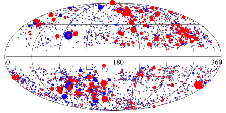
Figure 1: Peculiar velocity catalogue of 3456 spiral field galaxies, selected in the I-band and plotted in Galactic coordinates (taken from 2012). The red points are moving away from us and the blue points are moving towards us, with the size of the points proportional to the magnitude of the line-of-sight peculiar velocity.

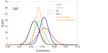
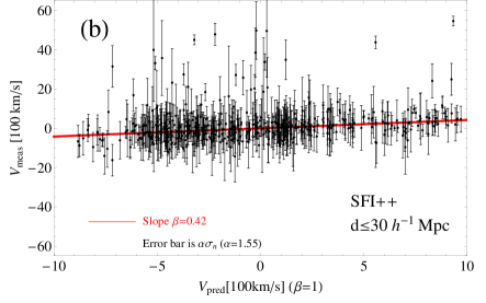
Figure 2: Panel (a): Posterior distribution of the linear flow parameter $\beta$ ($\equiv f/b$) for several surveys, together with a combined “hyper-parameter” analysis. Panel (b): comparison between measured peculiar velocities (from the SFI++ catalogue) and the smoothed reconstructed velocities (from the PSC$z$ galaxy redshift survey). Figure taken from (2012).

Equation (1) suggests that, in order to calculate the peculiar motion of a galaxy, one needs independently to measure the cosmological redshift, $z$, and the real distance, $r$ (in the same comoving frame). To determine the redshift, one uses spectroscopy, comparing features in the galaxy spectrum with known features in terrestrial spectra. Spectroscopic techniques are sufficiently mature that they produce negligible measurement error. On the other hand, determining the distance of a galaxy is considerably more difficult, because one needs to use an empirical relation between two intrinsic properties of a galaxy (or object within a galaxy, such as a supernova) to infer the distance. Among the most well used methods are the Tully-Fisher (hereafter TF) relation (, 1977) for spiral galaxies, the Fundamental Plane for elliptical galaxies (, 2010), and the luminosity-distance relation for Type-Ia supernovae (, 2003). Such distance estimates normally have much larger errors than spectroscopic redshifts (for more information on distance indicators, please see Appendix A).

In Fig. 1, we show the largest and densest peculiar velocity catalogue currently available. This is a close to full-sky sample of $3456$ spiral galaxies in the field and in galaxy groups. One can see that some peculiar velocities are positive, i.e. the galaxies are moving away from us (coloured red), while others are moving towards us (blue). The question is, what determines the motion of these galaxies?

In the standard $\Lambda$ cold dark matter (hereafter $\Lambda$CDM) cosmology, gravitational instability causes the growth of density perturbations and the emergence of the cosmic flow field. In the regime where the density perturbation is linear, the time evolution of the density contrast $\delta\equiv(\rho-\overline{\rho})/\rho$ and the galaxy peculiar velocity field are linked through the continuity equation (, 1993):

$$\vec{v}_{\rm g}(\vec{x})=\frac{H_{0}f_{0}}{4\pi}\int{\rm d}^{3}\vec{x}^{\prime}\delta_{\textrm{m}}(\vec{x}^{\prime},t_{0})\frac{(\vec{x}^{\prime}-\vec{x})}{\left|\vec{x}^{\prime}-\vec{x}\right|^{3}},$$ (2)

where $f_{0}\equiv{\rm d}\log(D(a))/{\rm d}\log(a)|_{a=1}$ is the present day growth rate, with $D(a)$ the growth factor describing how fast the density contrast grows. A complication is that galaxies and matter are related by some kind of bias parameter $b$, such that $\delta_{\rm g}=b\delta_{\rm m}$. This means that the relationship between $\vec{v}_{\rm g}$ and $\delta_{\rm m}$ is governed by the combination $f_{0}/b$, normally labelled $\beta$. Equation (2) can be adapted to provide at least two different kinds of test.

1. The velocity field ($v_{\rm g}$) is completely predictable given the underlying density distribution ($\delta_{\rm m}$). If we can measure both $v_{\rm g}$ and $\delta_{\rm m}$, we therefore can check the predictions of linear perturbation theory, and constrain cosmological parameters.

2. We can use Eq. (2) to compute the overall “streaming motion” of galaxies within a given volume. This can be compared with $\Lambda$CDM predictions of cosmic bulk motion as a function of scale and also used to test homogeneity.

The twin approaches, of comparing $\delta$ vs. $\vec{v}_{\rm g}$ and determining the bulk motion, have dominated this research area for over two decades (e.g. see previous reviews 1994, 2002). As a recent example, (2012) used the PSC$z$ (Point Source Catalogue of redshifts) sample (, 1995, 1999, 2000) to trace the underlying mass density field within $300\,{h^{-1}{\rm Mpc}}$, under the assumption of linear and deterministic bias. Then using this $\delta_{\rm m}(\vec{x})$ function the predicted velocity field can be compared with the measured velocities. By minimizing the deviations between the smoothed reconstructed velocities and the measured velocity catalogues (including the Early galaxy catalogue ENEAR, Bernardi et al. 2002, Spiral galaxies in SFI++ 2007 and two supernova catalogues, 2003 and 2012), constraints were placed on $\beta$, as shown in Fig. 2a. Different peculiar velocity catalogues give quite consistent constraints on $\beta$, and the velocity–velocity comparison is consistent with the predictions of $\Lambda$CDM (Fig. 2b). More detailed future comparisons between these two vector fields would then constitute tests of the gravitational instability paradigm and for the $\Lambda$CDM model (e.g. see the constraint on modified gravity models in 2012).

4 How large is the streaming motion?

Figure 3: A schematic illustration of bulk motion $\vec{u}$ and small scale velocity dispersion $\sigma_{\ast}$.

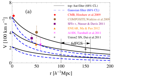
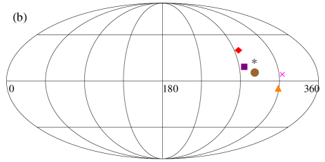
Figure 4: Panel (a): comparison between the bulk velocity amplitude and theoretical evaluation (Eq. (4)) for various catalogues and methods at difference depths. The theoretical expectation is given for two different choices of window function (top-hat in solid black and Gaussian in dashed blue), together with the $\pm 1\,\sigma$ expected scatter. Panel (b): direction of the bulk flow found using different data sets.

The above comparison tells us the extent to which the velocity field follows the mass-density field in the way predicted by the standard cosmology. The individual velocity modes, on the other hand, contain information both on large and small scales. To see this, consider a few galaxy samples on the sky (as shown schematically in Fig. 3), which may share the same streaming motion towards some particular direction, even while each of them has its own small-scale velocity. The bulk motion reflects the large-scale density perturbations, while the small-scale peculiar motions can be considered as a velocity dispersion arising from the local environment.

The straightforward way of calculating the bulk flow is to average all of the peculiar velocities out to survey depth $R$ as (, 2011)

$$\vec{V}_{\rm{bulk}}(R)=\int_{r<R}\vec{v}_{\rm{pec}}(\vec{x}){\rm d}^{3}x\left/\int_{r<R}{\rm d}^{3}x.\right.$$ (3)

However, since individual peculiar velocities $\vec{v}_{\rm{pec}}(\vec{x})$ are subject to both an intrinsic velocity dispersion ($\sigma_{\ast}$) and measurement error ($\sigma_{\rm n}$), it is hard to determine the left-hand-side of Eq. (3). Instead, a variety of methods have been developed to estimate the bulk flow given the measured radial velocities. Figure 4 shows the results of some bulk flow reconstructions on various scales, including: the observed CMB dipole that characterises our peculiar motion with respect to the CMB rest frame (, 2009); a “minimal weight” method for a composite galaxy catalogue as well as the Type-Ia supernovae catalogue (2009 and 2012); the inverse Tully-Fisher relation for the SFI++ catalogue (, 2011); and the Fundamental Plane method for the ENEAR catalogue (, 2014).

What is the amplitude of the bulk flow that we expect in the $\Lambda$CDM model and how certainly can it be predicted? The expected variance $\sigma_{V}$ of the bulk flow on a given scale can be calculated knowing the power spectrum of density perturbations and using Eqs. 2 and 3. The probability distribution of the bulk flow is a Maxwell-Boltzmann distribution, skewed towards higher velocities (Bahcall et al., 1994; Coles & Lucchine, 2002):

$$p(V){\rm d}V=\sqrt{\frac{54}{\pi}}\left(\frac{V}{\sigma_{V}}\right)^{2}e^{-3/2(V/\sigma_{V})^{2}}\left(\frac{{\rm d}V}{\sigma_{V}}\right).$$ (4)

The variance of the flow magnitude is also asymmetric, because of the non-Gaussian shape for the distribution.

Fig. 4a shows the most likely value and $\pm 1\,\sigma$ scatter of the bulk flow as a function of scale $R$, using two choices of smoothing function (top-hat and Gaussian). One can see that the size of bulk motion decreases with $R$, which is because more modes are averaged over in a larger volume. In addition, the scatter is larger for smaller scales, because of the increased sampling variance. It is also clear that the expected scatter means that bulk flow measurements can never be very strongly constraining. Nevertheless, they provide good tests of the standard picture. We certainly expect that for very large scales the Universe becomes homogeneous, and so as $R\rightarrow\infty$ the bulk velocity should be close to zero in the $\Lambda$CDM model. However, deviations from that model could give quite different predictions, e.g. if there were isocurvature-type initial perturbations, then it would be possible to have a large relative motion between the matter and CMB rest frames (Turner, 1991; , 2011).

The observational estimates plotted on Fig. 4 converge with the theoretical prediction out to $150\,{h^{-1}{\rm Mpc}}$, but at larger distance the situation is still not entirely clear. (2011) has argued that there is a “dark flow” with an amplitude around $1000\,{\rm km}{\rm s^{-1}}$ on scales of $z\simeq 0.2$, while recent results from the Planck satellite did not find such a flow (, 2013). Further information on large-scale bulk flows will come from the six-Degree-Field Galaxy Survey (6dFGS), which is probing the southern hemisphere out to $150\,{h^{-1}{\rm Mpc}}$ with the largest peculiar velocity survey yet constructed.

5 Tracing the missing baryons

   

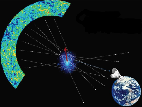
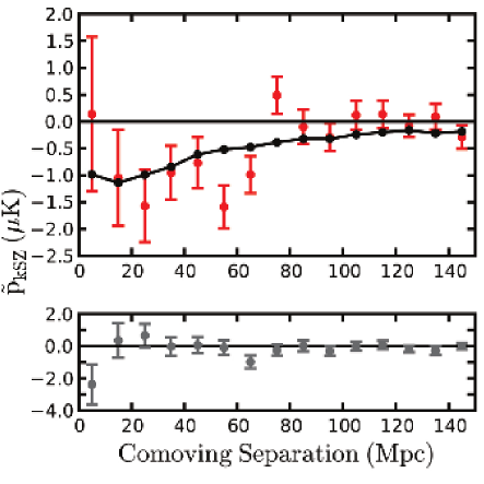
Figure 5: Left: illustration of the kinetic Sunyaev-Zeldovich (kSZ) effect. A small fraction of the CMB photons are scatter by hot gas in clusters of galaxies (and other structures), and Doppler shifted by the line of sight velocity of the scattering gas. Right: first statistical detection of the kSZ effect from the Atacama Cosmology Telescope (ACT), produced by averaging over the positions of galaxies. The red points are data, the black points are the expectation from numerical simulations (Sehgal et al., 2010) and the lower panel is a null test (taken from , 2012).

For traditional ways of estimating distance, the error increases as the objects get farther away, and hence it is increasingly difficult to estimate peculiar velocities for deeper samples and larger volumes. However, there is another entirely different method of estimating the line-of-sight peculiar velocity, which does not suffer from this distance-dependent uncertainty. This method is called the “kinetic Sunyaev-Zeldovich effect,” as first proposed by Sunyaev and Zeldovich in 1972 (Sunyaev & Zeldovich, 1972, 1980). The idea is shown in the left panel of Fig. 5. CMB photons travel to us from the last-scattering surface at $z\simeq 1100$, passing through all the intervening structures. Ionised gas in galaxy clusters (for example) can re-scatter a fraction of the CMB photons, Doppler shifting them to either higher or lower energy, depending on the line-of-sight peculiar velocity of the cluster. This causes an anisotropy on the CMB sky of amplitude

$$\frac{\delta T}{T}=\sigma_{\rm T}\int n_{\rm e}\left(\frac{v}{c}\right){\rm d}l,$$ (5)

where $n_{\rm e}$ is the electron density in the cluster, $v$ is the radial peculiar motion, $\sigma_{\rm T}$ is the cross-section of Compton scattering and $l$ integrates through the cluster. The effect is weak for an individual cluster, and has the same spectrum as the CMB itself (unlike the larger “thermal SZ effect”), making it difficult to extract. However, by knowing the positions of large-scale structures it is possible to measure an average effect. Upper limits from Planck have already placed constraints on the large-scale monopole and dipole, ruling out some speculative models (, 2013). Improvements in measurement techniques should allow interesting constraints to be placed on the peculiar motion $v$ of individual galaxy clusters.

In fact the kSZ effect was firstly detected statistically by (2012), who explored the CMB temperature map from the Atacama Cosmology Telescope (ACT) at the positions of $5000$ Sloan Digital Sky Survey samples (, 2006). By estimating the velocity differences between pairs of galaxies with separation distance $r$, and weighting the ACT map appropriately, (2012) were able to detect the average kSZ effect as a function of $r$ (shown in the right panel of Fig. 5).

The kSZ signal is not dominated by the very cores of clusters and hence is a direct probe of the “missing baryons” in the Universe. As assessed at low redshift by (2004), for example, the baryon fraction from identified sources – main sequence stars, stellar remnants, substellar objects and gas – adds up to only around 10% of the amount baryons known from cosmological studies. Theoretical considerations suggest that most of the undetected baryons are in gaseous form in the outskirts of virialised groups and clusters, and in the overdense filaments that connect them. Numerical simulations (Cen & Ostriker, 2006; Bregman, 2007) show that most of the baryons are effectively hiding in a phase with temperatures of $10^{5}$–$10^{7}\,$K (that is difficult to detect directly), in the Warm-Hot-Intergalactic-Medium (WHIM), which has overdensities in the range 1–1000. The kSZ effect essentially uses the CMB as a backlight to find those missing baryons, probing the outskirts of galaxy clusters and large-scale structure in general. Further study of cross-correlations between tracers of the gravitational potential and the gas (e.g. , 2014) hold great promise for teaching us more about the distribution of gas in the WHIM on larger scales than has previously been possible to probe.

6 Analysis tools

In order to use velocities to test cosmological paradigms and constrain parameters, it is necessary to develop analysis approaches that carefully control systematic uncertainties. Many different techniques have been introduced over the last 30 years. However, there are some signs that more recent methods might be offering distinct improvements. Cosmology is now dominated by Bayesian approaches to data analysis, with techniques derived from linear algebra being commonplace, so that likelihood functions and de-correlation studies become feasible. Such methods can be applied to compare velocity and density fields and examine bulk flows.

Burkey & Taylor (2004) discuss such approaches for reconstructing the peculiar veolocity power spectrum. (2009) describe how to combine multiple data sets using a minimum variance weighting scheme for constructing the bulk flow. (2011) use basis functions and the TF relation to compare velocity and density fields, as well as to calibrate uncertainties and hence determine $\beta$. (2012) discuss the use of a “hyper-parameter” technique for combining multiple noisy peculiar velocity data sets. These are just a few examples of the encouraging signs that statistical techniques are keeping pace with the improving quality of velocity data.

7 Conclusions

The study of peculiar velocities provides direct tests of several fundamental issues relating to structure formation. It is possible to examine the gravitational instability paradigm, as well as probing homogeneity and limiting non-Gaussianity. This is in addition to the use of velocities for yielding constraints on cosmological parameters, which was once the sole focus.

In the past the use of peculiar velocities has been hampered by the dominance of systematic uncertainties in estimates of the peculiar velocity field. New statistical analysis techniques and improved data, including the use of the kinetic Sunyaev-Zeldovich effect, mean that there is increasing interest in the use of peculiar velocities in cosmology. If this trend continues, then the next decade may see the promise of cosmic flows finally being fulfilled.

Appendix A Distance indicators

The Tully-Fisher (hereafter TF) relation (, 1977) is an example of a distance estimator for spiral galaxies. Spirals are flattened systems supported by rotation, with the rotational velocity well defined due to the flat rotation curves (, 1970). One expects bigger galaxies to rotate faster, and empirically there is an approximate power-law relating the luminosity and rotation speed. Hence, by measuring linewidths and apparent magnitudes one can estimate the distance of a galaxy. An analogous relation exists for elliptical galaxies, connecting luminosity and velocity dispersion and known as the Faber-Jackson relation (, 2010). An improved correlation for ellipticals comes from recognising a “fundamental plane” in the 3-dimensional space of surface brightness, velocity dispersion and effective radius. Tighter distance estimates can be found for galaxies with Type-Ia supernovae, since they have characteristic light curves, with the peak luminosity being effectively a constant, so that the peak apparent magnitude is a distance indicator.

Typically the supernova distances can have a scatter as small as 8%, while the best Tully-Fisher and Fundamental Plane distances have uncertainties of around 20%. Improving such distance estimates is crucial for obtaining better cosmological velocity constraints. However, more critical that the statistical scatter is controlling the systematic uncertainties; distance errors which correlate with galaxy properties or positions can lead to undesirable biases in velocity analyses. Hence reducing the systematic uncertainties requires large samples and analysis techniques which investigate (and correct for) such correlations.

References

- Bahcall et al. (1994) Bahcall N.A., Cen R., Gramann M., 1994, ApJ, 430, L13
- Bernardi et al. (2002) Bernardi M., Alonso M.V., da Costa L.N., Willmer C.N.A., Wegner G., Pellegrini P.S., Rite C., Maia M.A.G., 2002, AJ, 123, 2990
- (3) Branchini E., et al., 1999, MNRAS, 308, 1
- Bregman (2007) Bregman J.N., 2007, ARAA, 45, 221
- Burkey & Taylor (2004) Burkey D., Taylor A.N., 2004, MNRAS, 347, 255
- Cen & Ostriker (2006) Cen R., Ostriker J.P., 2006, ApJ, 650, 560
- Coles & Lucchine (2002) Coles P., Luccine F., 2002, Cosmology: The Origin and Evolution of Cosmic Structure, John Wiley & Sons, New York
- (8) Dai D.C., Kinney W.H., Stojkovic D., 2011, JCAP, 4, 15
- (9) Davis M., Nusser A., Masters K.L., Springob C., Huchra J.P., Lemson G., 2011, MNRAS, 413, 2906
- (10) Dekel A., et al., 1993, ApJ, 412, 1
- (11) Dekel A., 1994, ARAA, 32, 371
- (12) Faber S.M., Jackson R.E., 1976, ApJ, 204, 668
- (13) Fisher K., Huchra J., Strauss M., Davis M., Yahil A., Schlegel D., 1995, ApJ, 100, 69
- (14) Fukugita M., Peebles P.J.E., 2004, ApJ, 616, 643.
- (15) Gunn J.E., et al., 2006, ApJ, 131, 2332.
- (16) Hand N., et al. (Atacama Cosmology Telescope collaboration), 2012, PRL, 109, 041101
- (17) Hellwing W.A., Barreira A., Frenk C.S., Li B., Cole S., 2014, arXiv:1401.0706
- (18) Hinshaw G., et al., 2009, ApJS, 180, 225
- (19) Hudson M.J., Turnbull S.J., 2012, ApJL, 751, 30
- (20) Jones D.H., et. al, 2009, MNRAS, 399, 683
- (21) Kashlinsky A., et al., 2011, ApJ, 732, 1
- (22) Ma Y.Z., Branchini E., Scott D., 2012, MNRAS, 425, 2880
- (23) Ma Y.Z., Gordon C., Feldman H., 2011, PRD, 83, 103002
- (24) Ma Y.Z., Pan J., 2014, MNRAS, 437, 1996
- (25) Ma Y.Z., Scott D., 2013, MNRAS, 428, 2017.
- (26) Ma Y.Z., Taylor J.E., Scott D., 2013, MNRAS, 436, 2029.
- (27) Nusser A., Davis M., 2011, ApJ, 736,93
- (28) Peebles P.J.E., 1993, Principles of Physical Cosmology, Princeton University Press, Princeton
- (29) Planck Collaboraton Int. XIII, A&A, in press, arXiv: 1303.5090
- (30) Rubin V.C., Ford W.K., 1970, ApJ, 159, 379
- (31) Saunders W., et al., 2000, MNRAS, 317, 55
- Sehgal et al. (2010) Sehgal N., et al., 2010, ApJ, 709, 920.
- (33) Springob C.M., Masters K.L., Haynes M.P., Giovanelli R., Marinoni C., 2007, ApJS, 172, 599
- Sunyaev & Zeldovich (1972) Sunyaev R.A., Zeldovich Y.B., 1972, CoASP, 4, 173
- Sunyaev & Zeldovich (1980) Sunyaev R.A., Zeldovich Y.B., 1980, ARAA, 18, 537
- (36) Tonry J.L., et al., 2003, ApJ, 594, 1
- (37) Tully R.B., Fisher J.R., 1997, A&A, 54, 661
- (38) Turnbull S.J., Hudson M.J., Feldman H.A., Hicken M., Kirshner R.P., Watkins R., 2012, MNRAS, 420, 447
- Turner (1991) Turner M., 1991, PRD, 44, 3737
- (40) van Waerbeke L., Hinshaw G., Murray N., 2014, PRD, 89, 023508
- (41) Watkins R., Feldman H.A., Hudson M.J., 2009, MNRAS, 392, 743
- (42) Zaroubi S., 2002, in ‘Frontiers of the Universe’, ed. L. Celnikier & J. Tran Thanh Van, Tha Giai Publishers, Vietnam [arXiv:astro-ph/0206052]