SIMULATION AND ANALYTICAL APPROACH TO THE IDENTIFICATION

OF SIGNIFICANT FACTORS

Alexander V. Bulinski¹ and Alexander S. Rakitko ​​

Faculty of Mathematics and Mechanics, Lomonosov Moscow State University

Moscow 119991, Russia

bulinski@yandex.ru

Keywords: nonbinary random response; identification of significant factors; regularized estimates of prediction error; exchangeable random variables; central limit theorem.

ABSTRACT

We develop our previous works concerning the identification of the collection of significant factors determining some, in general, non-binary random response variable. Such identification is important, e.g., in biological and medical studies. Our approach is to examine the quality of response variable prediction by functions in (certain part of) the factors. The prediction error estimation requires some cross-validation procedure, certain prediction algorithm and estimation of the penalty function. Using simulated data we demonstrate the efficiency of our method. We prove a new central limit theorem for introduced regularized estimates under some natural conditions for arrays of exchangeable random variables.

1. INTRODUCTION

In a number of models the (random) response variable $Y$ depends on some factors $X_{1},\ldots,X_{n}$. A nontrivial problem is to identify the set of the most “significant factors”. Loosely speaking, for a given $r<n$ one can try to find such collection $\{k_{1},\ldots,k_{r}\}\subset\{1,\ldots,n\}$ that $Y$ depends “essentially” on $X_{k_{1}},\ldots,X_{k_{r}}$ and the impact of other factors can be viewed as negligible. Note that the problem of this type is important in medical and biological studies where $Y$ can describe the state of a patient health. For instance, $Y=1$ or $Y=-1$ may indicate that a person is sick or healthy, respectively. Note also that in pharmacological studies the values $-1$ or $1$ of a response variable can describe efficient or inefficient application of some medicine. Thus it is clear that binary response variables play an important role in various disciplines. At the same time it is obvious that more detailed description of experiments can be desirable. In this regard we refer, e.g., to Bulinski and Rakitko (2014) where non-binary response variables were studied.

There exist various complementary approaches concerning the prediction of response variable and selection of significant combinations of factors. Such analysis in medical and biological studies is included in special research domain called the genome-wide association studies (GWAS). The problems and progress in this important domain are considered, e.g., in Moore et al. (2010) and Visscher et al. (2012). Among powerful statistical tools applied in GWAS one can indicate the principle component analysis (Lee et al. (2012)), logistic and logic regression (Schwender and Ruczinski (2010), Sikorska et al. (2013)), LASSO (Tibshirani and Taylor (2012)) and various methods of statistical learning (Hastie et al. (2008)). Note also that there are various modifications of these methods.

We are interested in the “dimensionality reduction” of the whole collection of factors and so employ the term “MDR method”. This term was introduced, for binary response variable, in the paper Ritchie et al. (2001) and goes back to the Michalski algorithm. However, instead of considering contiguity tables (to specify zones of low and high risk) presented in Ritchie et al. (2001) and many subsequent works we choose another way. Namely, to predict (in general non-binary) $Y$ we use some function $f$ in factors $X_{1},\ldots,X_{n}$. The quality of such $f$ is determined by means of the error function $Err(f)$ involving a penalty function $\psi$. This penalty function allows us to take into account the importance of different values of $Y$. As the law of $Y$ and $X=(X_{1},\ldots,X_{n})$ is unknown we cannot evaluate $Err(f)$. Thus statistical inference is based on the estimates of error function. Developing Bulinski et al. (2012), Bulinski (2012), Bulinski (2014) we propose (in more general setting) statistics constructed by means of a prediction algorithm for response variable and $K$-fold cross-validation procedure. One of the main results of Bulinski and Rakitko (2014) gives the criterion of strong consistency of the mentioned error function estimates when the number of observations tends to infinity. The strong consistency is essential because to identify the “significant collection” of factors we have to compare simultaneously a number of statistics. Moreover, we proposed in Bulinski (2014) and Bulinski and Rakitko (2014) the regularized versions of the employed statistics (involving the appropriate estimates of the penalty function) to establish the central limit theorem (CLT).

The paper is organized as follows. Section 2 contains notation and auxiliary results. In Section 3 we discuss the results of simulations to identify (according to our method) the collection of significant factors determining a binary response variable. In Section 4 we prove the new CLT for our estimates (in general for non-binary response $Y$) using some natural conditions concerning the arrays of exchangeable random variables.

2. NOTATION AND AUXILIARY RESULTS

Further on we suppose that all random variables under consideration are defined on a probability space $(\Omega,\mathcal{F},{\sf P})$. Let $Y$ take values in a finite set $\mathbb{Y}$ which we will identify with the set $\{-m,\ldots,m\}$ where $m\in\mathbb{N}$. To comprise binary variables we can assume that their values belong to the set $\{-1,0,1\}$ and the value $0$ is taken with probability $0$. Let also $X_{1},\ldots,X_{n}$ take values in an arbitrary finite set $\mathbb{X}=\{0,\ldots,s\}$. Choose $f:\mathbb{X}\to\mathbb{Y}$ and a penalty function $\psi:\mathbb{Y}\to\mathbb{R}_{+}$. The trivial case $\psi\equiv 0$ is excluded. Introduce the error function

$$Err(f):={\sf E}|Y-f(X)|\psi(Y).$$

It is easily seen that one can write $Err(f)$ in the following way

$$Err(f)=\sum_{y,z\in\mathbb{Y}}|y-z|\psi(y){\sf P}(Y=y,f(X)=z)=\sum_{z\in\mathbb{Y}}\sum_{x\in A_{z}}w^{\top}(x)q(z)$$

where $q(z)$ is the $z$-th column of $(2m+1)\times(2m+1)$ matrix $Q$ with entries $q_{y,z}=|y-z|$, $y,z\in\mathbb{Y}$ (the entry $q_{-m,-m}$ is located at the left upper corner of $Q$),

$$w(x)=(\psi(-m){\sf P}(Y=-m,X=x),\ldots,\psi(m){\sf P}(Y=m,X=x))^{\top}$$

and $\top$ stands for transposition. All vectors are considered as column-vectors. According to Bulinski and Rakitko (2014) we can rewrite $Err(f)$ as follows

$$Err(f)=\sum_{i=0}^{2m-1}\sum_{i-m<|y|\leq m}\psi(y){\sf P}(Y=y,|f(X)-y|>i).$$ (1)

The law of $(X,Y)$ is unknown, therefore, for each $f:\mathbb{X}\to\mathbb{Y}$, we can not evaluate $Err(f)$. Thus it is natural that statistical inference concerning the quality of prediction of the response variable $Y$ by means of $f(X)$ is based on the estimates of $Err(f)$.

Let $\xi^{1},\xi^{2},\ldots$ be a sequence of independent identically distributed (i.i.d.) random vectors having the same law as $(X,Y)$. For $N\in\mathbb{N}$, set $\xi_{N}=(\xi^{1},\ldots,\xi^{N})$. We will use approximation of $Err(f)$ by means of $\xi_{N}$ (as $N\to\infty$) and a prediction algorithm (PA). This PA employs a function $f_{PA}=f_{PA}(x,\xi_{N})$ defined for $x\in\mathbb{X}$ and $\xi_{N}$ and taking values in $\mathbb{Y}$. More exactly, we operate with a family of functions $f_{PA}(x,v_{p})$ (with values in $\mathbb{Y}$) defined for $x\in\mathbb{X}$ and $v_{p}\in(\mathbb{X}\times\mathbb{Y})^{p}$ where $p\in\mathbb{N}$, $p\leq N$. To simplify the notation we write $f_{PA}(x,v_{p})$ instead of $f_{PA}^{p}(x,v_{p})$. For $S\subset\{1,\ldots,N\}$ we set $\xi_{N}(S)=\{\xi^{j},j\in S\}$ and $\overline{S}:=\{1,\ldots,N\}\setminus S$. For $K\in\mathbb{N}$ $(K>1)$, introduce a partition of a set $\{1,\ldots,N\}$ by means of subsets

$$S_{k}(N)=\{(k-1)[N/K]+1,\ldots,k[N/K]\mathbb{I}\{k<K\}+N\mathbb{I}\{k=K\}\},\leavevmode\nobreak\ k=1,\ldots,K,$$

here $[a]$ is the integer part of a number $a\in\mathbb{R}$. Following Bulinski (2012) we can construct an estimate of $Err(f)$ involving $\xi_{N}$, prediction algorithm defined by $f_{PA}$ and $K$-cross-validation (on cross-validation we refer, e.g., to Arlot and Celisse (2010)). Namely, set

$$\widehat{Err}_{K}(f_{PA},\xi_{N}):=\sum_{i=0}^{2m-1}\sum_{i-m<|y|\leq m}\frac{1}{K}\sum_{k=1}^{K}\sum_{j\in S_{k}(N)}\frac{\widehat{\psi}(y,\xi_{N}({S_{k}(N)}))\mathbb{I}\{A_{N}(y,i,k,j)\}}{\sharp S_{k}(N)}$$ (2)

where $A_{N}(y,i,k,j)=\{Y^{j}\!=\!y,|f_{PA}(X^{j},\xi_{N}(\overline{S_{k}(N)}))\!-\!y|>i\}$. Here, for each $k\in\{1,\ldots,K\}$, let $\widehat{\psi}(y,\xi_{N}({S_{k}(N)}))$ be strongly consistent estimates of $\psi(y)$ (as $N\to\infty$) for all $y\in\mathbb{Y}$, i.e.

$$\widehat{\psi}(y,\xi_{N}({S_{k}(N)}))\to\psi(y)\;\;\mbox{a.s.},\;\;y\in\mathbb{Y},\;\;N\to\infty.$$

In Bulinski and Rakitko (2014) the criterion was established to guarantee the relation

$$\widehat{Err}_{K}(f_{PA},\xi_{N})\to Err(f)\;\;\mbox{a.s.},\;\;N\to\infty.$$

For $r\in\{1,\ldots,n\}$ set $\mathbb{X}_{r}=\{0,1\ldots,s\}^{r}$. Then $\mathbb{X}=\mathbb{X}_{n}$. We write $\alpha=(k_{1},\ldots,k_{r})$, $X_{\alpha}=(X_{k_{1}},\ldots,X_{k_{r}})$ and $x_{\alpha}=(x_{k_{1}},\ldots,x_{k_{r}})$ where $x_{i}\in\{0,\ldots,s\}$, $i=1,\ldots,n$. In many models it is natural to assume that $Y$ depends only on some collection of factors $X_{\alpha}$. We say that a vector $\alpha$ (and the corresponding vector $X_{\alpha}$) is significant if, for $x\in\mathbb{X}$ and $y\in\mathbb{Y}$, one has ${\sf P}(Y=y|X=x)={\sf P}(Y=y|X_{\alpha}=x_{\alpha})$ whenever ${\sf P}(X=x)>0$. In Bulinski and Rakitko (2014) (formula (14)), for each $\beta=(m_{1},\ldots,m_{r})$ with $1\leq m_{1}<\ldots<m_{r}\leq n$, the function $f^{\beta}$ was introduced and (formula (19)) prediction algorithm $\widehat{f}^{\beta}(x,\xi_{N}(W_{N}))$ was proposed where $x\in\mathbb{X}$ and $\xi_{N}(W_{N})=(\xi_{n_{1}},\ldots,\xi_{n_{u}})$, $W_{N}=\{n_{1},\ldots,n_{u}\}\subset\{1,\ldots,N\}$. It was proved (Theorem 2 in Bulinski and Rakitko (2014)) that if $\alpha=(k_{1},\ldots,k_{r})$ is significant then, for any $\beta=(m_{1},\ldots,m_{r})$ and each $\nu>0$, one has $\widehat{Err}_{K}(\widehat{f}^{\alpha}_{PA},\xi_{N})\leq\widehat{Err}_{K}(\widehat{f}^{\beta}_{PA},\xi_{N})+\nu$ a.s. for all $N$ large enough. Thus it is reasonable to choose among all $\beta=(m_{1},\ldots,m_{r})$ such vector $\alpha$ that $\alpha={\sf argmin}_{\beta}\{\widehat{Err}_{K}(\widehat{f}^{\beta}_{PA},\xi_{N})\}$ or take for further analysis (using permutation tests, see, e.g., Golland et al. (2005)) several vectors giving the estimated prediction error close to the minimal value. Moreover, for specified sequence $\varepsilon=(\varepsilon_{N})_{N\in\mathbb{N}}$ of positive numbers, the regularized versions $\widehat{f}^{\beta}_{PA,\varepsilon}$ of $\widehat{f}^{\beta}_{PA}$ were introduced and the CLT was established (Theorem 3 in Bulinski and Rakitko (2014)) for these estimates. Further extension of such CLT is obtained in Section 4 of the present paper.

3. SIMULATION

To illustrate our approach we consider three examples. For each example we simulated i.i.d. random vectors $\xi_{1},\ldots,\xi_{N}$. Then (for each example) we evaluated the estimate $\widehat{Err}_{K}(\widehat{f}^{\beta}_{PA,\varepsilon},\xi_{N})$ where $K=10$, vector $\beta$ had appropriate dimension, and for regularization of estimates we employed $\varepsilon_{N}=N^{-1/4}$, $N\in\mathbb{N}$. After that we took all possible collections $\beta$ of $r$ factors among $n$ and selected $10$ of them with lowest values of estimated prediction error $\widehat{Err}_{K}(\widehat{f}^{\beta}_{PA,\varepsilon},\xi_{N})$. For saving time of calculations we used $n=50$ factors. However the results are interesting and instructive. Let the factors $X_{i}$, $i=1,\ldots,n$, be i.i.d. random variables taking values $-1,0,1$ with probabilities $1/3$ and $Y$ be a binary response variable with values $-1$ and $1$. We assume also that $r$ (the cardinality of the collection of significant factors) is equal to 3 in Example 1 and equals 4 in Examples 2 and 3. In Examples 1 and 2 the impact of the “noise” on response variable is described by means of multiplication of $Y$ by the random variable $(-1)^{Z_{\gamma}}$ where $Z_{\gamma}$ is the Bernoulli random variable, namely, ${\sf P}(Z_{\gamma}=1)=\gamma$ and ${\sf P}(Z_{\gamma}=0)=1-\gamma$. We consider $\gamma=0.1$, that is the mean level of noise is $10\%$. Assume that $Z_{\gamma}$ and $X=(X_{1},\ldots,X_{n})$ are independent.

Example 1. Let $r=3$ and $Y=Y^{0}\cdot(-1)^{Z_{\gamma}}$ where

$$Y^{0}=\begin{cases}\;\;1,\leavevmode\nobreak\ \leavevmode\nobreak\ \leavevmode\nobreak\ &X_{2}=1,\leavevmode\nobreak\ X_{3}\geq 0,\vspace{-0.3cm}\\ \;\;1,&X_{2}=-1,\leavevmode\nobreak\ X_{3}+X_{5}\geq 1,\vspace{-0.3cm}\\ -1,\leavevmode\nobreak\ \leavevmode\nobreak\ \leavevmode\nobreak\ &\text{otherwise}.\end{cases}$$

Here $X_{2},X_{3},X_{5}$ are the factors determining $Y$.

Example 2. Take $r=4$ and set $Y=Y^{0}\cdot(-1)^{Z_{\gamma}}$ where

$$Y^{0}=\begin{cases}\;\;1,\leavevmode\nobreak\ \leavevmode\nobreak\ \leavevmode\nobreak\ &X_{2}=1,\vspace{-0.3cm}\\ \;\;1,&X_{3}+X_{5}+X_{8}\geq 2,\vspace{-0.3cm}\\ -1,\leavevmode\nobreak\ \leavevmode\nobreak\ \leavevmode\nobreak\ &\text{otherwise}.\end{cases}$$

The factors determining $Y$ are $X_{2},X_{3},X_{5},X_{8}$.

In the following example we consider nonlinear constrains.

Example 3. Let $r=4$. Set

$$Y=\begin{cases}\;\;1,\leavevmode\nobreak\ \leavevmode\nobreak\ \leavevmode\nobreak\ &3^{X_{1}+X_{2}+X_{4}}\sin(X_{3}Z^{\ln(X_{3}-2X_{4}+7)})>1,\vspace{-0.3cm}\\ -1,\leavevmode\nobreak\ \leavevmode\nobreak\ \leavevmode\nobreak\ &\text{otherwise,}\end{cases}$$

assuming the random variable $Z$ be uniformly distributed on $[0,1]$. Let $Z$ and $X$ be independent. Here $X_{1},X_{2},X_{3},X_{4}$ are the factors determining $Y$.

Collections of various factors and corresponding values of $\widehat{Err}_{K}(\widehat{f}^{\beta}_{PA,\varepsilon},\xi_{N})$ obtained for $N=500$ are presented in Tables 1, 2 and 3. Namely, $EPE_{i}$ stands for $\widehat{Err}_{K}$ found in the framework of Example $i$ where $i=1,2,3$. Columns $n_{1},n_{2},n_{3}$ (and $n_{1},n_{2},n_{3},n_{4}$) in the tables indicate the choice of factors $X_{n_{1}},X_{n_{2}},X_{n_{3}}$ (and $X_{n_{1}},X_{n_{2}},X_{n_{3}},X_{n_{4}}$), respectively. The same information is provided in Tables 4, 5 and 6 where one has $N=1000$.

It is worth to emphasize that in all considered examples for large ($N=1000$) and rather modest ($N=500$) samples our method permits to identify correctly the collections of significant factors (corresponding to the minimum of prediction error estimates). Moreover, these tables show that the estimated prediction error for significant collections of factors has visible advantage w.r.t. other collections.

$n_{1}$	$n_{2}$	$n_{3}$	$EPE_{1}$
2	3	5	0.6336
2	3	32	0.8020
2	3	48	0.8100
2	3	28	0.8260
2	3	4	0.8515
2	3	31	0.8527
2	3	22	0.8528
2	3	34	0.8551
2	3	50	0.8649
2	3	23	0.8652

Table 1: $r=3$, N=500

$n_{1}$	$n_{2}$	$n_{3}$	$n_{4}$	$EPE_{2}$
2	3	5	8	0.3997
2	3	5	24	0.5901
2	3	5	46	0.5911
2	3	5	32	0.5961
2	3	5	31	0.6014
2	3	5	10	0.6059
2	3	5	14	0.6224
2	3	5	42	0.6250
2	3	5	29	0.6251
2	3	5	22	0.6267

Table 2: $r=4$, N=500

$n_{1}$	$n_{2}$	$n_{3}$	$n_{4}$	$EPE_{3}$
1	2	3	4	0.0939
1	3	20	42	0.2956
2	3	5	29	0.3211
1	3	4	39	0.3228
1	2	3	8	0.3322
1	3	24	42	0.3355
1	2	3	5	0.3395
1	2	3	20	0.3431
1	2	3	40	0.3487
1	2	3	27	0.3558

Table 3: $r=4$, N=500

$n_{1}$	$n_{2}$	$n_{3}$	$EPE_{1}$
2	3	5	0.5675
2	3	32	0.7981
2	3	47	0.8096
2	3	34	0.8126
2	3	4	0.8127
2	3	44	0.8334
2	3	48	0.8369
2	3	22	0.8401
2	3	23	0.8441
2	3	31	0.8442

Table 4: $r=3$, N=1000

$n_{1}$	$n_{2}$	$n_{3}$	$n_{4}$	$EPE_{2}$
2	3	5	8	0.4768
2	3	5	42	0.6936
2	5	8	11	0.6970
2	5	8	26	0.6974
2	3	5	6	0.6981
2	5	8	12	0.7035
2	5	8	50	0.7039
2	3	5	32	0.7045
2	3	5	27	0.7060
2	3	5	46	0.7063

Table 5: $r=4$, N=1000

$n_{1}$	$n_{2}$	$n_{3}$	$n_{4}$	$EPE_{3}$
1	2	3	4	0.2278
2	3	4	32	0.3355
1	2	3	6	0.4352
1	2	3	46	0.4663
1	3	4	15	0.4694
1	2	3	27	0.4697
1	2	3	50	0.4704
2	3	4	18	0.4812
2	3	4	44	0.4856
1	3	4	40	0.4862

Table 6: $r=4$, N=1000

However, if $N$ is not large enough the proposed stochastic approach can lead to the choice of a collection of factors which is not (the most) significant. For instance, if $N=500$ then the right identifications of significant factors have occurred in $99\%$, $97\%$, $69\%$ of respective simulations for Examples 1, 2 and 3 (averaging is over 100 performance procedures). In Example 3 this frequency of right identification increases till $93\%$ when $N=1000$.

Figures 1, 2 and 3 demonstrate for each example the character of stabilization of $\widehat{Err}_{K}$ fluctuations as $N$ grows. This stabilization of estimates can be explained not only by their strong consistency but also on account of their asymptotic normality. In this regard we concentrate further on the new conditions which guarantee the CLT validity for proposed prediction error estimates.

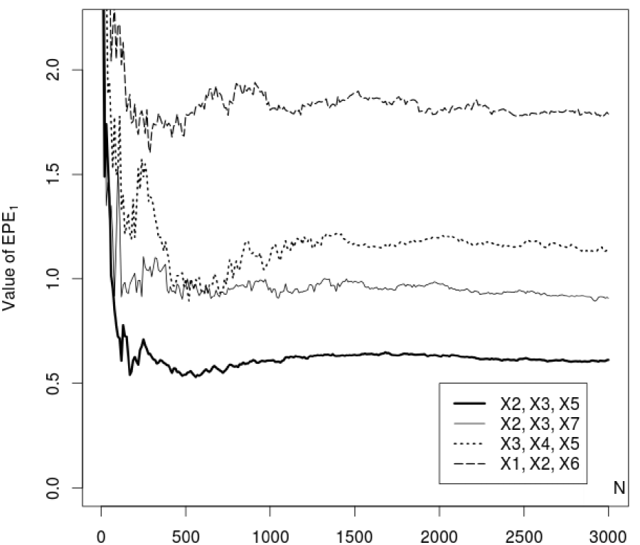
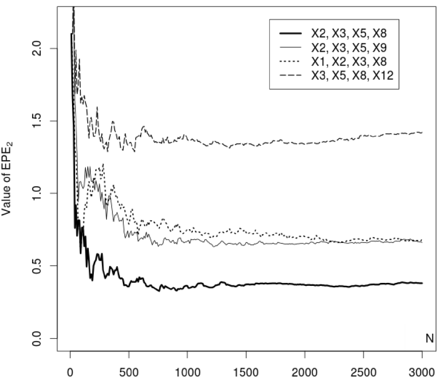
Figure 1: Simulations corresponding to Example 1.

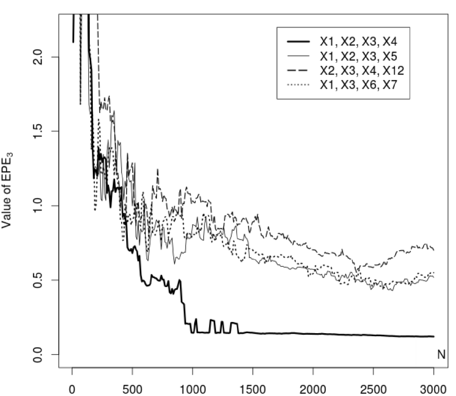
Figure 2: Simulations corresponding to Example 2.

Figure 3: Simulations corresponding to Example 3.

4. NEW VERSION OF THE CENTRAL LIMIT THEOREM

We proved in Bulinski and Rakitko (2014) that asymptotic distribution of random variables $\sqrt{N}(\widehat{Err}_{K}(f_{PA},\xi_{N})-Err(f))$ coincides with the limit law of

$$\sqrt{N}(\widehat{T}_{N}(f)-Err(f))=\dfrac{\sqrt{N}}{K}\sum_{k=1}^{K}\sum_{i=0}^{2m-1}\sum_{i-m<|y|\leq m}\dfrac{1}{\sharp S_{k}(N)}\sum_{j\in S_{k}(N)}h_{N}(y,i,k,j),$$ (3)

as $N\to\infty$, where

$$h_{N}(y,i,k,j)=\widehat{\psi}(y,{S_{k}(N)})\mathbb{I}\{Y^{j}=y,|f(X^{j})-y|>i\}-\psi(y){\sf P}(Y=y,|f(X)-y|>i)$$

and $\widehat{\psi}(y,{S_{k}(N)}):=\widehat{\psi}(y,\xi_{N}(S_{k}(N)))$.

Evidently the summands here are not independent in view of the presence of $\widehat{\psi}(\cdot,{S_{k}(N)})$. To prove the CLT for random variables appearing in (3) we used in Bulinski and Rakitko (2014) the hypothesis of asymptotic normality of the vector consisting of two subvectors, one of them being $\sqrt{N}(\widehat{\psi}(\cdot,{S_{k}(N)})-\psi(\cdot))$. Now we employ another approach assuming symmetry of the estimates $\widehat{\psi}(\cdot,{S_{k}(N)})$ of a penalty function. Recall the following

Definition 1.

A collection of random variables $(X_{1},\ldots,X_{n})$, $n\in\mathbb{N}$, is called exchangeable if, for any permutation $\sigma\in S(n)$ of the set $\{1,\ldots,n\}$, one has

$$Law(X_{1},\ldots,X_{n})=Law(X_{\sigma(1)},\ldots,X_{\sigma(n)}).$$

Take $K\in\mathbb{N}$ and suppose that $N/K=q$ where $q\in\mathbb{N}$. Thus $\sharp S_{k}(N)=q$ for each $k=1,\ldots,K$. Consider the sequence of $K\times q$ matrices $(C^{(N)})_{N\in\mathbb{N}}$ with entries

$$\xi^{(N)}_{k,j}:=\sum_{i=0}^{2m-1}\sum_{i-m<|y|\leq m}\widehat{\psi}(y,S_{k}(N))\cdot\mathbb{I}\{Y^{j+(k-1)q}=y,|f(X^{j+(k-1)q})-y|>i\}$$ (4)

where $k=1,\ldots,K$ and $j=1,\ldots,q$. Introduce

$$X_{N,j}:=\dfrac{1}{\sqrt{K}}\sum_{k=1}^{K}\xi_{k,j}^{(N)},\leavevmode\nobreak\ \leavevmode\nobreak\ \leavevmode\nobreak\ j=1,\ldots,q.$$ (5)

Then

$$\sqrt{N}(\widehat{T}_{N}(f)-Err(f))=\frac{1}{\sqrt{q}}\sum_{j=1}^{q}(X_{N,j}-\sqrt{K}Err(f)).$$ (6)

We take the functions $\widehat{\psi}(y,\cdot)$ which are symmetric for each $y\in\mathbb{Y}$. Then any row and any column of $C^{(N)}$ contain exchangeable random variables (row-column exchangeability). Clearly, the triangular array $\{X_{N,j},\leavevmode\nobreak\ 1\leq j\leq q,N\in\mathbb{N}\}$ is row-wise exchangeable.

We will establish the CLT for sums appearing in (6). In Berti et al. (2004) one can find several results which guarantee the CLT validity when the summands $\{X_{i}\}_{i=1}^{n}$ are (in appropriate manner) conditionally identically distributed. Namely,

$$\dfrac{1}{\sqrt{n}}\big{(}f(X_{1})+\ldots+f(X_{n})-L_{n}\big{)}\xrightarrow{law}Z_{0,\sigma^{2}}\sim\mathcal{N}(0,\sigma^{2})$$ (7)

where $f$ is a measurable function such that ${\sf E}|f(X_{1})|<\infty$ and $L_{n}=L_{n}(X_{1},\ldots,X_{n})$. In the mentioned paper the authors applied the martingale techniques. Such approach was developed for exchangeable variables in Weber (1980). We will prove the CLT in the form (7) with $f(x)=x$ for row-wise exchangeable arrays by means of other tools. We will employ the recent result of Röllin (2013). Let ${\sf Y}=(Y_{1},\ldots,Y_{m})$ be a collection of exchangeable random variables such that

$${\sf E}Y_{1}=0,\leavevmode\nobreak\ \leavevmode\nobreak\ \leavevmode\nobreak\ {\sf E}|Y_{1}|^{3}<\infty.$$ (8)

Consider $\Sigma=(\sigma_{i,j})_{1\leq i,j\leq m}$ with $\sigma_{i,j}={\sf E}(Y_{i}Y_{j})$, i.e. the covariance matrix of $\sf Y$. Set $\sigma_{i,i}=\sigma^{2}$. Suppose that $Y_{1}+\ldots+Y_{m}=C_{m}$ a.s. where $C_{m}$ is a constant. Then w.l.g. we can assume that

$$\sum_{i=1}^{m}Y_{i}=0\leavevmode\nobreak\ \leavevmode\nobreak\ \leavevmode\nobreak\ {a.s.}$$ (9)

For a function $h:\mathbb{R}^{d}\rightarrow\mathbb{R}$ and $k\in\mathbb{N}$ set

$$C_{h}^{(k)}:=\max_{i_{1},\ldots,i_{d}\geq 0,\sum_{j=1}^{d}i_{j}=k}\left\|\frac{\partial^{k}h}{\partial x_{1}^{i_{1}}\ldots\partial x_{d}^{i_{d}}}\right\|_{\infty}.$$

Theorem 1 (Röllin (2013)).

Let $\sf Y$ be a vector consisting of exchangeable random variables and having a covariance matrix $\Sigma$. Assume that conditions (8) and (9) are satisfied. Then

$$|{\sf E}h({\sf Y})-{\sf E}h({\sf Z})|\leq C_{h}^{(2)}\Big{[}{\sf var}\Big{(}\sum_{i=1}^{m}Y_{i}^{2}\Big{)}\Big{]}^{\frac{1}{2}}+16mC_{h}^{(3)}{\sf E}|Y_{1}|^{3}$$ (10)

where ${\sf Z}\sim\mathcal{N}(0,\Sigma)$.

For an array $\{X_{n,i},1\leq i\leq k_{n},n\in\mathbb{N}\}$ we will use the following notation

$$\widehat{\mu}_{k_{n}}:=\dfrac{1}{k_{n}}\sum_{i=1}^{k_{n}}X_{n,i},\;\;\;\;\widehat{\sigma}^{2}_{k_{n}}:=\dfrac{1}{k_{n}}\sum_{i=1}^{k_{n}}(X_{n,i}-\widehat{\mu}_{k_{n}})^{2}.$$ (11)

We apply (10) to prove the following result.

Lemma 1.

Let $\{X_{n,i},1\leq i\leq k_{n},n\in\mathbb{N}\}$ be a row-wise exchangeable array where positive integers $k_{n}\to\infty$ as $n\to\infty$. Suppose that    $1^{\circ}\!.\;\;\sup_{n\in\mathbb{N}}{\sf E}X_{n,1}^{4}<\infty,$    $2^{\circ}\!.\;\;{\sf E}X_{n,1}^{2}-{\sf E}X_{n,1}X_{n,2}\to\sigma^{2}>0,\;n\to\infty,$    $3^{\circ}\!.\;\;{\sf cov}(X_{n,1}^{2},X_{n,2}^{2})+{\sf cov}(X_{n,1}X_{n,2},X_{n,3}X_{n,4})-2\,{\sf cov}(X_{n,1}^{2},X_{n,2}X_{n,3})\to 0,\;n\to\infty.$ Then, for any sequence $(m_{n})_{n\in\mathbb{N}}$ of positive integers such that $m_{n}\to\infty$ and $m_{n}/k_{n}\to\alpha<1$ as $n\to\infty$, the following relation holds

$$\dfrac{1}{\sqrt{m_{n}}}\sum_{i=1}^{m_{n}}(X_{n,i}-\widehat{\mu}_{k_{n}})\xrightarrow{law}Z_{0,(1-\alpha)\sigma^{2}}\sim\mathcal{N}(0,(1-\alpha)\sigma^{2}),\;\;n\to\infty.$$

Proof. First of all, for each $n\in\mathbb{N}$, we introduce the auxiliary random variables

$$Y_{n,i}:=X_{n,i}-\widehat{\mu}_{k_{n}},\leavevmode\nobreak\ \leavevmode\nobreak\ \leavevmode\nobreak\ i=1,\ldots,k_{n}.$$

The collection $\{Y_{n,1},\ldots,Y_{n,k_{n}}\}$ is exchangeable as $\{X_{n,1},\ldots,X_{n,k_{n}}\}$ has this property. Obviously $\sum_{i=1}^{k_{n}}Y_{n,i}=0$ a.s. for any $n\in\mathbb{N}$. Moreover, ${\sf E}Y_{n,1}=0,$ for any $n\in\mathbb{N}$. One can verify that

$${\sf E}Y_{n,1}^{2}=\left(1-\frac{1}{k_{n}}\right)({\sf E}X_{n,1}^{2}-{\sf E}X_{n,1}X_{n,2}),\;\;\;{\sf E}Y_{n,1}Y_{n,2}=-\,\frac{1}{k_{n}}({\sf E}X_{n,1}^{2}-{\sf E}X_{n,1}X_{n,2}).$$

For each $n\in\mathbb{N}$, take a vector ${\bf Z}=(Z_{n,1},\ldots,Z_{n,m_{n}})$ independent of $(X_{n,1},\ldots,X_{n,k_{n}})$ and such that ${\bf Z}\sim\mathcal{N}(0,\Sigma)$. Here $\Sigma$ is a covariance matrix of ${\bf Y}=(Y_{n,1},\ldots,Y_{n,m_{n}})$. Thus ${\sf cov}(Z_{n,i},Z_{n,j})={\sf cov}(Y_{n,i},Y_{n,j})$, $1\leq i,j\leq m_{n}$. Clearly,

$$\dfrac{1}{\sqrt{m_{n}}}\sum_{i=1}^{m_{n}}(X_{n,i}-\widehat{\mu}_{k_{n}})=\frac{1}{\sqrt{m_{n}}}\sum_{i=1}^{m_{n}}Y_{n,i}=:S_{{\bf Y},m_{n}}.$$

Set $S_{{\bf Z},m_{n}}:=\frac{1}{\sqrt{m_{n}}}\sum_{i=1}^{m_{n}}Z_{n,i}.$ In view of $2^{\circ}$ condition $m_{n}/k_{n}\to\alpha$ ($n\to\infty$) yields

$${\sf var}S_{{\bf Z},m_{n}}={\sf E}Y_{n,1}^{2}+(m_{n}-1){\sf E}Y_{n,1}Y_{n,2}=\left(1-\dfrac{m_{n}}{k_{n}}\right)({\sf E}X_{n,1}^{2}-{\sf E}X_{n,1}X_{n,2})\to(1-\alpha)\sigma^{2}.$$

Consequently, $S_{{\bf Z},m_{n}}\stackrel{{\scriptstyle law}}{{\longrightarrow}}\mathcal{N}(0,(1-\alpha)\sigma^{2}),\;\;n\to\infty.$ Now we show that $S_{{\bf Y},m_{n}}$ and $S_{{\bf Z},m_{n}}$ have the same limit distribution. Due to Theorem 7.1 Billingsley (1968) it is sufficient to verify that

$${\sf E}f(S_{{\bf Y},m_{n}})-{\sf E}f(S_{{\bf Z},m_{n}})\to 0,\leavevmode\nobreak\ \leavevmode\nobreak\ \leavevmode\nobreak\ n\to\infty,$$ (12)

for any three times continuously differentiable function $f:\mathbb{R}\to\mathbb{R}$ such that

$$c_{f}^{(j)}:=\left\|\frac{d^{j}f}{dx^{j}}\right\|_{\infty}<\infty,\;\;j=1,2,3.$$

For any fixed $n\in\mathbb{N}$, apply Theorem 1 with $m=m_{n}$, $Y_{i}=\frac{1}{\sqrt{m_{n}}}Y_{n,i}$, $i=1,\ldots,m_{n}$, and

$$h(x_{1},\ldots,x_{m_{n}}):=f(x_{1}+\ldots+x_{m_{n}}).$$

Then we can write

$$\big{|}{\sf E}f(S_{{\bf Y},m_{n}})-{\sf E}f(S_{{\bf Z},m_{n}})\big{|}=\big{|}{\sf E}h({\bf Y})-{\sf E}h({\bf Z})\big{|}$$

$$\leq C_{f}^{(2)}m_{n}^{-1}\Big{[}{\sf var}\Big{(}\sum_{i=1}^{m_{n}}Y_{n,i}^{2}\Big{)}\Big{]}^{\frac{1}{2}}+16C_{f}^{(3)}m_{n}^{-1/2}{\sf E}|Y_{n,1}|^{3}.$$

Note that

$${\sf var}\Big{(}\sum_{i=1}^{m_{n}}Y_{n,i}^{2}\Big{)}=m_{n}{\sf E}Y_{n,1}^{4}+m_{n}(m_{n}-1){\sf E}Y_{n,1}^{2}Y_{n,2}^{2}-m_{n}^{2}\big{(}{\sf E}Y_{n,1}^{2}\big{)}^{2}$$

$$=m_{n}\big{(}{\sf E}Y_{n,1}^{4}-({\sf E}Y_{n,1}^{2})^{2}\big{)}+m_{n}(m_{n}-1){\sf cov}(Y_{n,1}^{2},Y_{n,2}^{2}).$$

We claim that

$${\sf cov}(Y_{n,1}^{2},Y_{n,2}^{2})-\Big{[}{\sf cov}(X_{n,1}^{2},X_{n,2}^{2})+{\sf cov}(X_{n,1}X_{n,2},X_{n,3}X_{n,4})-2{\sf cov}(X_{n,1}^{2},X_{n,2}X_{n,3})\Big{]}\to 0$$

as $n\to\infty$. Indeed, set $S_{n}=\frac{1}{k_{n}}\sum_{i=1}^{k_{n}}X_{n,i}$. Using exchangeability property of $(X_{n,1},\ldots,X_{n,k_{n}})$ and taking into account that covariance function is bilinear we obtain

$${\sf cov}(Y_{n,1}^{2},Y_{n,2}^{2})={\sf E}Y_{n,1}^{2}Y_{n,2}^{2}-({\sf E}Y_{n,1}^{2})^{2}$$

$$={\sf cov}(X_{n,1}^{2},X_{n,2}^{2})+2\,{\sf cov}(X_{n,1}^{2},S_{n}^{2})-4\,{\sf cov}(X_{n,1}^{2},X_{n,2}S_{n})$$

$$-4\,{\sf cov}(X_{n,1}S_{n},S_{n}^{2})+4\,{\sf cov}(X_{n,1}S_{n},X_{n,2}S_{n})+{\sf cov}(S_{n}^{2},S_{n}^{2}).$$

For $n\to\infty$, by virtue of $1^{\circ}$ we get

$${\sf cov}(X_{n,1}^{2},S_{n}^{2})={\sf cov}(X_{n,1}^{2},X_{n,2}X_{n,3})+O(k_{n}^{-1}),$$

$${\sf cov}(X_{n,1}^{2},X_{n,2}S_{n})={\sf cov}(X_{n,1}^{2},X_{n,2}X_{n,3})+O(k_{n}^{-1}),$$

$${\sf cov}(X_{n,1}S_{n},S_{n}^{2})={\sf cov}(X_{n,1}X_{n,2},X_{n,3}X_{n,4})+O(k_{n}^{-1}),$$

$${\sf cov}(X_{n,1}S_{n},X_{n,2}S_{n})={\sf cov}(X_{n,1}X_{n,2},X_{n,3}X_{n,4})+O(k_{n}^{-1}).$$

Therefore, condition $3^{\circ}$ implies that ${\sf cov}(Y_{n,1}^{2},Y_{n,2}^{2})\to 0$ as $n\to\infty$. Thus relation (12) holds and the proof is complete. $\square$

Remark 1.

Assume that

$$\sup_{n\in\mathbb{N}}{\sf E}\big{(}(X_{n,1}-\widehat{\mu}_{k_{n}})/\widehat{\sigma}_{k_{n}}\big{)}^{4}<\infty.$$

Then, for a sequence $(m_{n})_{n\in\mathbb{N}}$ appearing in Lemma 1, one can prove the following version of the CLT

$$\dfrac{1}{\sqrt{m_{n}}}\sum_{i=1}^{m_{n}}\Big{(}\dfrac{X_{n,i}-\widehat{\mu}_{k_{n}}}{\widehat{\sigma}_{k_{n}}}\Big{)}\stackrel{{\scriptstyle law}}{{\longrightarrow}}Z_{0,1-\alpha}\sim\mathcal{N}(0,1-\alpha),\leavevmode\nobreak\ \leavevmode\nobreak\ \leavevmode\nobreak\ n\to\infty.$$

Remark 2.

In Chernoff and Teicher (1958) the result similar to Lemma 1 was established but the important case $\alpha=0$ (which we consider further) was not comprised. One can also employ the martingale approach of Weber (1980) to obtain the result of Lemma 1. However Rollin’s Theorem 1 permits us to estimate the convergence rate to the limit Gaussian law. Moreover, we can prove that under certain conditions the asymptotic behavior of the specified partial sums is described by the mixture of the normal laws.

Now we consider the triangular array $\{X_{N,i},1\leq i\leq q,N\in\mathbb{N}\}$ with elements defined by (5). Thus we take $k_{n}=q$ in Lemma 1 and write $N$ instead of $n$.

Lemma 2.

Suppose that, for each $N\in\mathbb{N}$, any $y\in\mathbb{Y}$ and all $k=1,\ldots,K$,

$$\sup_{y\in\mathbb{Y},\;N\in\mathbb{N},\;k\in\{1,\ldots,K\}}{\sf E}\left(\widehat{\psi}(y,S_{k}(N))\right)^{4}<\infty.$$ (13)

Let $(m_{N})_{N\in\mathbb{N}}$ be a sequence of positive integers such that $m_{N}\leq q$, $m_{N}\to\infty$ and$m_{N}/N\to\alpha<1$ as $N\to\infty$. Then

$$\dfrac{1}{\sqrt{m_{N}}}\sum_{i=1}^{m_{N}}(X_{N,i}-\widehat{\mu}_{N})\xrightarrow{law}Z_{0,(1-\alpha)\sigma^{2}}\sim\mathcal{N}(0,(1-\alpha)\sigma^{2})$$

where $\mu_{N}$ is introduced in (11) $($with $k_{n}=q$ and $n$ replaced by $N)$ and

$$\sigma^{2}\!=\!{\sf E}\left[\sum_{i=0}^{2m-1}\sum_{i-m<|y|\leq m}\psi(y)(\mathbb{I}\{Y\!=\!y,|f(X)-y|\!>\!i\}-{\sf P}(Y\!=\!y,|f(X)-y|\!>\!i))\right]^{2}\!\!.$$ (14)

Proof. We show that conditions of Lemma 1 are met. $1^{\circ}$ follows by virtue of (3), (5) and (13) as indicator function takes values in the set $\{0,1\}$. Now we turn to $2^{\circ}$. The exchangeability of the columns of the array $\{\xi^{(N)}_{k,j}\}$ implies that

$${\sf E}X_{N,1}X_{N,2}=\dfrac{1}{K}{\sf E}\left(\sum_{k=1}^{K}\xi^{(N)}_{k,1}\right)\left(\sum_{k=1}^{K}\xi^{(N)}_{k,2}\right)={\sf E}\xi_{1,1}^{(N)}\xi_{1,2}^{(N)}+(K-1){\sf E}\xi^{(N)}_{1,1}\xi^{(N)}_{2,2}.$$

The Lebesgue theorem on majorized convergence yields that the limit behavior of ${\sf E}\xi_{1,1}^{(N)}\xi_{1,2}^{(N)}$ as $N\to\infty$ will be the same as for ${\sf E}\zeta_{1,1}^{(N)}\zeta_{1,2}^{(N)}$ where

$$\zeta_{k,j}^{(N)}:=\sum_{i=0}^{2m-1}\sum_{i-m<|y|\leq m}\psi(y)\,\mathbb{I}\{Y^{j+(k-1)q}=y,|f(X^{j+(k-1)q})-y|>i\}.$$

Random vectors $(X^{1},Y^{1}),(X^{2},Y^{2}),\ldots$ are independent. Therefore, ${\sf E}\zeta_{1,1}^{(N)}\zeta_{1,2}^{(N)}={\sf E}\zeta_{1,1}^{(N)}{\sf E}\zeta_{1,2}^{(n)}$ and in view of (1) we get

$$\lim_{N\to\infty}{\sf E}\xi^{(N)}_{1,1}\xi^{(N)}_{1,2}=\lim_{N\to\infty}\big{(}{\sf E}\zeta_{1,1}^{(N)}\big{)}^{2}=\big{(}Err(f)\big{)}^{2}.$$

In a similar way we come to the relation

$$\lim_{N\to\infty}{\sf E}\xi^{(N)}_{1,1}\xi^{(N)}_{2,2}=\lim_{N\to\infty}\big{(}{\sf E}\zeta_{1,1}^{(N)}\big{)}^{2}=\big{(}Err(f)\big{)}^{2}.$$

Thus ${\sf E}X_{N,1}X_{N,2}\to K\big{(}Err(f)\big{)}^{2}$ as $N\to\infty$. Applying the Lebesgue theorem once again we conclude that

$$\lim_{N\to\infty}{\sf E}(X_{N,j})^{2}=\lim_{N\to\infty}{\sf E}(Z_{N,j})^{2}=\lim_{N\to\infty}\Big{[}{\sf E}(\zeta^{(N)}_{1,1})^{2}+(K-1){\sf E}\zeta^{(N)}_{1,1}\zeta^{(N)}_{1,2}\Big{]},$$

where

$$Z_{N,j}:=\dfrac{1}{\sqrt{K}}\sum_{k=1}^{K}\zeta_{k,j}^{(N)},\leavevmode\nobreak\ \leavevmode\nobreak\ \leavevmode\nobreak\ j=1,\ldots,q.$$

Taking into account that ${\sf E}\zeta^{(N)}_{1,1}\zeta^{(N)}_{1,2}=\big{(}Err(f)\big{)}^{2}$ (for each $N\geq 2K$) we get

$$\sigma^{2}={\sf E}\Big{[}\sum_{i=0}^{2m-1}\sum_{i-m<|y|\leq m}\psi(y)\,\mathbb{I}\{Y=y,|f(X)-y|>i\}\Big{]}^{2}-\big{(}Err(f)\big{)}^{2}$$

$$={\sf E}\left[\sum_{i=0}^{2m-1}\sum_{i-m<|y|\leq m}\psi(y)\big{(}\mathbb{I}\{Y=y,|f(X)-y|>i\}-{\sf P}(Y=y,|f(X)-y|>i)\big{)}\right]^{2}\!.$$

To complete the proof we verify condition $3^{\circ}$. Due to the Lebesgue theorem

$$\lim_{N\to\infty}{\sf Cov}(X_{N,1}^{2},X_{N,2}^{2})=\lim_{k\to\infty}{\sf Cov}(Z_{k,1}^{2},Z_{k,2}^{2})=0$$

as $Z_{k,1}$ and $Z_{k,2}$ are independent. Quite similar arguments justify the following relations ${\sf Cov}(X_{N,1}X_{N,2},X_{N,3}X_{N,4})\to 0$ and ${\sf Cov}(X_{N,1}^{2},X_{N,2}X_{N,3})\to 0$ as $N\to\infty$. $\square$

Let us discuss the established result. Instead of the initial task to study asymptotic behavior of $\sqrt{N}(\widehat{T}_{N}(f)-Err(f))$ we are able to specify the limit law for difference of two estimates of $Err(f)$. Namely, set

$$\widehat{L}_{m_{N}}=\dfrac{1}{m_{N}}\sum_{j=1}^{m_{N}}\dfrac{1}{\sqrt{K}}\sum_{k=1}^{K}\sum_{i=0}^{2m-1}\sum_{i-m<|y|\leq m}\Big{[}\widehat{\psi}(y,S_{k}(N))\cdot\mathbb{I}\{Y^{j+(k-1)q}=y,|f(X^{j+(k-1)q})-y|>i\}\Big{]}$$

and introduce $\widehat{L}_{q}$ by the same formula with $q$ instead of $m_{n}$. Then Lemma 2 affirms that $\sqrt{m_{N}}(\widehat{L}_{m_{N}}-\widehat{L}_{q})\stackrel{{\scriptstyle law}}{{\longrightarrow}}Z_{0,(1-\alpha)\sigma^{2}}\sim\mathcal{N}(0,(1-\alpha)\sigma^{2})$ as $N\to\infty$. Therefore, if we provide conditions to guarantee that $\sqrt{m_{N}}\big{(}\widehat{L}_{q}-Err(f)\big{)}\xrightarrow{{\sf P}}0$ then we can construct the approximate confidence intervals for $Err(f)$. We demonstrate that this is possible for regularized statistics introduced in Bulinski and Rakitko (2014) to identify the significant collections of factors.

For a sequence of random variables $(\eta_{N})_{N\in\mathbb{N}}$ we write $\eta_{N}=O_{\sf P}(1)$ if, for any $\gamma>0$, there exists $M(\gamma)>0$ such that ${\sf P}(|\eta_{N}|\geq M(\gamma))\leq\gamma$ for all $N$ large enough. Let $(m_{N})_{N\in\mathbb{N}}$ be a sequence of positive integers such that $m_{N}\leq q$ for $q=[N/K]$ and

$$m_{N}\to\infty,\;\;m_{N}/N\to 0,\;\;\mbox{as}\;\;N\to\infty.$$

Theorem 2.

Let $(m_{N})_{N\in\mathbb{N}}$ be a sequence introduced above. Assume that $\varepsilon=(\varepsilon_{N})_{N\in\mathbb{N}}$ is a sequence of positive numbers such that $\varepsilon_{N}\to 0$ and $m_{N}^{1/2}\varepsilon_{N}\to\infty$ as $N\to\infty$. Take any vector $\beta=(k_{1},\ldots k_{r})$ with $1\!\leq\!k_{1}\!<\!\ldots\!<\!k_{r}\!\leq\!n$, the corresponding function $f=f^{\beta}$ and the prediction algorithm defined by $f_{PA}=\widehat{f}_{PA,\varepsilon}^{\beta}$. Let, for any $y\in\mathbb{Y}$ and $k\in\{1,\ldots,K\}$, the estimate $\widehat{\psi}(y,S_{k}(N))$ be strongly consistent and

$$\sqrt{\sharp S_{k}(N)}(\widehat{\psi}(y,S_{k}(N))-\psi(y))=O_{{\sf P}}(1),\;\;N\to\infty.$$ (15)

Let also (13) hold. Then, as $N\to\infty$,

$$\sqrt{m_{N}}\Big{(}\dfrac{1}{m_{N}}\sum_{j=1}^{m_{N}}\dfrac{1}{\sqrt{K}}\sum_{k=1}^{K}\sum_{i=0}^{2m-1}\sum_{i-m<|y|\leq m}\Big{[}\widehat{\psi}(y,S_{k}(N))\mathbb{I}\{A_{N}(i,j,k,y)\}\Big{]}\!-\!Err(f)\Big{)}\stackrel{{\scriptstyle law}}{{\longrightarrow}}Z_{0,\sigma^{2}}.$$

Here $A_{N}(i,j,k,y)=\{Y^{j+(k-1)q}=y,|f_{PA}(X^{j+(k-1)q})-y|>i\}$, $Z_{0,\sigma^{2}}\sim\mathcal{N}(0,\sigma^{2})$ and $\sigma^{2}$ was introduced in (14).

Proof. One can show that

$$\sqrt{m_{N}}\big{(}\widehat{L}_{q}-Err(f)\big{)}$$

$$-\,\dfrac{\sqrt{m_{N}}}{\sqrt{K}}\sum_{k=1}^{K}\sum_{i=0}^{2m-1}\sum_{i-m<|y|\leq m}\Big{[}(\widehat{\psi}(y,{S_{k}(N)})-\psi(y)){\sf P}(Y=y,|f(X)-y|>i)$$

$$+\,\psi(y)\Big{(}\dfrac{1}{\sharp S_{k}(N)}\sum_{j\in S_{k}(N)}H_{N}(y,i,j)\Big{)}\Big{]}\xrightarrow{{\sf P}}0$$

as $N\to\infty$. Here $H_{N}(y,i,j)=\mathbb{I}\{Y^{j}=y,|f(X^{j})-y|>i\}-{\sf P}(Y=y,|f(X)-y|>i)$. For any $i\in\{0,\ldots,2m-1\}$ and $y\in\mathbb{Y}$, the CLT for arrays of i.i.d. random variables with finite second moment implies that

$$\dfrac{1}{\sqrt{\sharp S_{k}(N)}}\sum_{j\in S_{k}(N)}H_{N}(y,i,j)=O_{{\sf P}}(1),\;\;\;N\to\infty.$$

Since $m_{N}/\sharp S_{k}(N)\to 0$ we get

$$\dfrac{\sqrt{m_{N}}}{\sqrt{K}}\sum_{k=1}^{K}\sum_{i=0}^{2m-1}\sum_{i-m<|y|\leq m}\psi(y)\dfrac{1}{\sharp S_{k}(N)}\sum_{j\in S_{k}(N)}H_{N}(y,i,j)\xrightarrow{{\sf P}}0,\;\;\;N\to\infty.$$

In a similar way in view of (15) one has

$$\dfrac{\sqrt{m_{N}}}{\sqrt{K}}\sum_{k=1}^{K}\sum_{i=0}^{2m-1}\sum_{i-m<|y|\leq m}\big{(}\widehat{\psi}(y,{S_{k}(N)})-\psi(y)\big{)}{\sf P}(Y=y,|f(X)-y|>i)\xrightarrow{{\sf P}}0,\;\;\;N\to\infty.$$

Thus under conditions of Theorem 2 the asymptotic behavior of $\sqrt{m_{N}}\big{(}\widehat{L}_{m_{N}}-\widehat{L}_{q}\big{)}$ is the same as for $\sqrt{m_{N}}\big{(}\widehat{L}_{m_{N}}-Err(f)\big{)}$. $\square$

In Velez et al. (2007) the following choice of the penalty function $\psi$ was proposed

$$\psi(y)=\dfrac{c}{{\sf P}(Y=y)},\;\;y\in\mathbb{Y},\;\;c=\text{const}>0.$$

This choice was justified in Bulinski (2012) for binary response $Y$. We will employ this penalty function for nonbinary response as well, i.e. when $\mathbb{Y}=\{-m,\ldots,0,\ldots,m\}$. Futher we assume that ${\sf P}(Y=y)>0$ for all $y\in\mathbb{Y}$ and w.l.g. $c=1$.

Introduce $A_{N}(y,S_{k}(N))=\{Y^{j}\neq y,\;j\in S_{k}(N)\},\;N\in\mathbb{N},\;k\in\{1,\ldots,K\},\;y\in\mathbb{Y}$ and set (as usual $0/0:=0$)

$$\widehat{{\sf P}}_{S_{k}(N)}(Y=y):=\dfrac{\sum_{j\in S_{k}(N)}\mathbb{I}\{Y^{j}=y\}}{\sharp S_{k}(N)},\;\;\widehat{\psi}(y,S_{k}(N)):=\dfrac{\mathbb{I}\{\Omega\setminus A_{N}(y,S_{k}(N))\}}{\widehat{{\sf P}}_{S_{k}(N)}(Y=y)}.$$ (16)

Corollary 1.

The estimate $\widehat{\psi}$ defined by (16) satisfies conditions of Theorem 2.

Proof. Fix arbitrary $y\in\mathbb{Y}$ and $k=1,\ldots,K$. One can easily check that $\widehat{\psi}(y,S_{k}(N))$ is a strongly consistent estimate of $\psi(y)$. Moreover, by CLT for arrays of i.i.d. random variables we have

$$\sqrt{\sharp\,S_{k}(N)}\big{(}\widehat{{\sf P}}_{S_{k}(N)}(Y=y)-{\sf P}(Y=y)\big{)}\xrightarrow{law}Z_{0,\sigma_{1}^{2}(y)}\sim\mathcal{N}\big{(}0,\sigma_{1}^{2}(y)\big{)},\;\;\;N\to\infty,$$

where $\sigma_{1}^{2}(y)={\sf P}(Y=y)(1-{\sf P}(Y=y))$. Taking into account that $\widehat{{\sf P}}_{S_{k}(N)}(Y\!=\!y)\!\to\!{\sf P}(Y\!=\!y)$ a.s. and $\sqrt{S_{k}(N)}\mathbb{I}\{A_{N}(y,S_{k}(N))\}\xrightarrow{\sf P}0$ as $N\to\infty$, one can write by Slutsky’s lemma that

$$\sqrt{\sharp S_{k}(N)}\big{(}\widehat{\psi}_{S_{k}(N)}(y)-\psi(y)\big{)}\xrightarrow{law}Z_{0,\sigma_{2}^{2}(y)}\sim\mathcal{N}\big{(}0,\sigma_{2}^{2}(y)\big{)},\;\;\;N\to\infty,$$

where $\sigma_{2}^{2}(y)=(1-{\sf P}(Y=y)){\sf P}(Y=y)^{-3}$. Thus (15) holds. Now we verify (13). Clearly, $\widehat{\psi}(y,S_{k}(N))\leq\sharp S_{K}(N)$ for any $N\in\mathbb{N}$. Put $\varepsilon:=\min_{y\in\mathbb{Y}}{\sf P}(Y=y)$. Then by the Hoeffding inequality

$${\sf E}|\widehat{\psi}(y,S_{k}(N))|^{4}={\sf E}\Big{[}|\widehat{\psi}_{N,k}(y)|^{4}\mathbb{I}\Big{\{}\big{|}\widehat{{\sf P}}_{S_{k}(N)}(Y=y)-{\sf P}(Y=y)\big{|}>\varepsilon/2\Big{\}}\Big{]}$$

$$+{\sf E}\Big{[}(\widehat{\psi}(y,S_{k}(N)))^{4}\mathbb{I}\Big{\{}\big{|}\widehat{{\sf P}}_{S_{k}(N)}(Y=y)-{\sf P}(Y=y)\big{|}\leq\varepsilon/2\Big{\}}\Big{]}$$

$$\leq 2(\sharp S_{K}(N))^{4}\exp\{-\sharp S_{1}(N)\varepsilon^{2}/2\}+2^{4}/\varepsilon^{4}.$$

Thus we come to (13). $\square$

To simplify notation we will write in the following theorem $\widehat{Err}_{K}(f_{PA},\xi_{N})$ for random variable introduced in (2) replacing $\widehat{\psi}(y,S_{k}(N))$ by $\widehat{\psi}(y,\overline{S_{k}(N)})$, $y\in\mathbb{Y}$, $k=1,\ldots,K$. After such replacement in (4) – (6) we obtain the new row-wise exchangeable array $\{X_{N,j},1\leq j\leq q,N\in\mathbb{N}\}$ and therefore all established results hold true in this case.

Theorem 3.

Let $\varepsilon_{N}\to 0$ and $N^{1/2}\varepsilon_{N}\to\infty$ as $N\to\infty$. Then, for each $K\in\mathbb{N}$, any vector $\beta=(k_{1},\ldots k_{r})$ with $1\leq k_{1}<\ldots<k_{r}\leq n$, the corresponding function $f=f^{\beta}$ and prediction algorithm defined by $f_{PA}=\widehat{f}_{PA,\varepsilon}^{\beta}$, the following relation holds:

$$\sqrt{N}(\widehat{Err}_{K}(f_{PA},\xi_{N})-Err(f))\stackrel{{\scriptstyle law}}{{\longrightarrow}}Z_{0,\sigma^{2}}\sim\mathcal{N}(0,\sigma^{2}),\;\;N\to\infty.$$ (17)

Here $\sigma^{2}$ is variance of the random variable

$$V=\sum_{i=0}^{2m-1}\sum_{i-m<|y|\leq m}\frac{\mathbb{I}\{Y=y\}}{{\sf P}(Y=y)}\left(\mathbb{I}\{|f(X)-y|>i\}-{\sf P}(|f(X)-y|>i\big{|}Y=y)\right).$$ (18)

Proof. Set, for $f:\mathbb{X}\to\mathbb{Y}$ and $N\in\mathbb{N}$,

$$T_{N}(f):=\dfrac{1}{K}\sum_{k=1}^{K}\dfrac{1}{\sharp S_{k}(N)}\sum_{i=1}^{2m-1}\sum_{i-m<|y|\leq m}\psi(y)\sum_{j\in S_{k}(N)}\mathbb{I}\{Y^{j}=y,|f(X^{j})-y|>i\}.$$

The Slutsky lemma shows that the limit behavior of the random variables introduced in (3) will be the same as for random variables

$$\rho_{N}:=\sqrt{N}(T_{N}(f)-Err(f))$$

$$-\,\frac{\sqrt{N}}{K}\sum_{k=1}^{K}\sum_{i=0}^{2m-1}\sum_{i-m<|y|\leq m}\frac{(\widehat{\sf P}_{\overline{S_{k}(N)}}(Y=y)-{\sf P}(Y=y)){\sf P}(Y=y,|f(X)-y|>i)}{{\sf P}(Y=y)^{2}}$$

$$=\frac{\sqrt{N}}{K}\sum_{k=1}^{K}\sum_{i=0}^{2m-1}\sum_{i-m<|y|\leq m}\frac{1}{\sharp\,S_{k}(N)}\sum_{j\in S_{k}(N)}\frac{\mathbb{I}\{Y^{j}=y,|f(X^{j})-y|>i)}{{\sf P}(Y=y)}$$

$$-\,\frac{\sqrt{N}}{K}\sum_{k=1}^{K}\sum_{i=0}^{2m-1}\sum_{i-m<|y|\leq m}\frac{1}{\sharp\,\overline{S_{k}(N)}}\sum_{j\in\overline{S_{k}(N)}}\mathbb{I}\{Y^{j}=y\}\frac{{\sf P}(Y=y,|f(X)-y|>i\}}{({\sf P}(Y=y))^{2}}.$$

Let $a_{k},b_{k}$, $k=1,\ldots,K$, be any real numbers. We use the following simple observation

$$\frac{1}{\sharp\,S_{k}(N)}\sum_{k=1}^{K}a_{k}+\frac{1}{\sharp\,\overline{S_{k}(N)}}\sum_{l=1,\ldots,K;l\neq k}b_{l}=\sum_{k=1}^{K}\left(\frac{a_{k}}{\sharp\,S_{k}(N)}+b_{k}\sum_{l=1,\ldots,K;l\neq k}\frac{1}{\sharp\,\overline{S_{l}(N)}}\right).$$

Combining the latter formulas we can write

$$\rho_{N}=\frac{\sqrt{N}}{K}\sum_{k=1}^{K}\sum_{j\in S_{k}(N)}\left(\frac{V^{j}_{1}}{\sharp\,S_{k}(N)}+V^{j}_{2}\sum_{l=1,\ldots,K;l\neq k}\frac{1}{\sharp\,\overline{S_{l}(N)}}\right)$$

where

$$V^{j}_{1}=\sum_{i=0}^{2m-1}\sum_{i-m<|y|\leq m}\frac{\mathbb{I}\{Y^{j}=y,|f(X^{j})-y|>i\}}{{\sf P}(Y=y)},$$

$$V^{j}_{2}=-\sum_{i=0}^{2m-1}\sum_{i-m<|y|\leq m}\frac{\mathbb{I}\{Y^{j}=y\}{\sf P}(Y=y,|f(X)-y|>i)}{({\sf P}(Y=y))^{2}}.$$

Take any $k\in\{1,\ldots,K\}$ and employ CLT for an array of bounded centered i.i.d. random variables $\{V^{j}_{1}+V^{j}_{2},j\in S_{k}(N),N\in\mathbb{N}\}$. Then

$$\frac{1}{\sqrt{\sharp\,S_{k}(N)}}\sum_{j\in S_{k}(N)}(V^{j}_{1}+V^{j}_{2})\stackrel{{\scriptstyle law}}{{\longrightarrow}}Z_{0,\sigma^{2}}\sim\mathcal{N}(0,\sigma^{2}),\;\;N\to\infty,$$

where $\sigma^{2}={\sf var}(V_{1}^{j}+V_{2}^{j})$. Note now that, for each $k=1,\ldots,K$,

$$\frac{N}{\sharp\,S_{k}(N)}\to\frac{1}{K},\;\;\;\sum_{l=1,\ldots,K;l\neq k}\frac{N}{\sharp\,\overline{S_{l}(N)}}\to\frac{1}{K},\;\;\;N\to\infty.$$

For each $N\in\mathbb{N}$, the families of random variables $\{V^{j}_{1}+V^{j}_{2},j\in S_{k}(N)\}$, $k=1,\ldots,K$, are independent. Thus we come to the following relation

$$\rho_{N}\stackrel{{\scriptstyle law}}{{\longrightarrow}}Z_{0,\sigma^{2}}\sim\mathcal{N}(0,\sigma^{2}),\;\;N\to\infty.$$

Obviously we can write $\sigma^{2}={\sf var}\,V$ where $V$ is introduced in (18). The proof is complete. $\square$

Remark 3.

It is not difficult to construct the consistent estimates $\widehat{\sigma}_{N}$ of unknown $\sigma$ appearing in (17). Therefore (if $\sigma^{2}\neq 0$) we can claim that under conditions of Theorem 3

$$\frac{\sqrt{N}}{\widehat{\sigma}_{N}}(\widehat{E}rr_{K}(f_{PA},\xi_{N})-Err(f))\stackrel{{\scriptstyle law}}{{\longrightarrow}}\frac{Z}{\sigma}\sim\mathcal{N}(0,1),\;\;N\to\infty.$$

Remark 4.

It is interesting to compare Theorem 3 with simulations corresponding to Example 3 when $N$ is rather small (e.g., $N=200$). In this case the choice of $\widehat{\psi}(y,\overline{S_{k}(N)})$ can lead to better identification of significant factors.

BIBLIOGRAPHY

Arlot, S., Celisse, A. (2010). A survey of cross-validation procedures for model selection. Statist. Surv.. 4, 40–79.

Berti, Patrizia; Pratelli, Luca; Rigo, Pietro. (2004). Limit theorems for a class of identically distributed random variables. Ann. Probab. 32, no. 3, 2029–2052.

Billingsley P. (1968). Convergence of Probability Measures. John Wiley $\&$ Sons Inc., New York.

Bulinski, A.V. (2014). On foundation of the dimensionality reduction method for explanatory variables. J. Math. Sci., DOI 10.1007/s10958-014-1838-7.

Bulinski, A.V. (to appear, 2014). Central limit theorem related to MDR method.: Proceedings of the Fields Institute International Symposium on Asymptotic Methods in Stochastics, in Honour of Miklós Csörgő’s Work on the occasion of his anniversary. arXiv:1301.6609 [math.PR].

Bulinski, A., Butkovsky, O., Sadovnichy, V., Shashkin, A., Yaskov, P., Balatskiy, A., Samokhodskaya, L., Tkachuk, V. (2012). Statistical methods of SNP data analysis and applications. Open Journal of Statistics. 2(1), 73–87.

Bulinski A.V., Rakitko A.S. (2014). Estimation of nonbinary random response. Dokl. Math., 455(6), 1–5.

Chernoff, H., Teicher, H. (1958). A Central Limit Theorem for Sums of Interchangeable Random Variables. Ann. Math. Statist. 29(1),118–130.

Golland, P., Liang, F., Mukherjee, S., Panchenko, D. (2005). Permutation Tests for Classification. LNCS, 3559, 501–515.

Hastie T., Tibshirani R. and Friedman J. (2008). The Elements of Statistical Learning; Data Mining, Inference and Prediction. Springer, New York. Second edition.

Lee S., Epstein M.P., Duncan R. and Lin X. (2012). Sparse Principal Component Analysis for Identifying Ancestry-Informative Markers in Genome Wide Association Studies. Genet. Epidemiol. 36, 293–302.

Moore J.B., , Asselbergs F.W. and Williams S.M. (2010). Bioinformatics challenges for genome-wide association studies. Bioinformatics. 26, 445–455.

Ritchie, M.D., Hahn, L.W., Roodi, N., Bailey, R.L., Dupont, W.D., Parl, F.F., Moore, J.H. (2001). Multifactor-dimensionality reduction reveals high-order interactions among estrogen-metabolism genes in sporadic breast cancer. Am. J. Hum Genet. 69(1), 138–147.

Röllin, A. (2013). Stein’s method in high dimensions with applications. Ann. Inst. Henri Poincaré Probab. Stat. 49(2), 529–549.

Schwender, H., Ruczinski, I. (2010). Logic regression and its extensions. Adv. Genet.. 72, 25-45.

Sikorska K., Lesaffre E., Groenen P.F.G., and Eilers P.H.C. (2013). GWAS on your notebook: fast semi-parallel linear and logistic regression for genome-wide association studies. BMC Bioinformatics, 14:166.

Tibshirani R.J. and Taylor J. (2012). Degrees of freedom in lasso problems. Ann. Statist. 40, 1198–1232.

Velez, D.R., White, B.C., Motsinger, A.A., Bush, W.S., Ritchie, M.D., Williams, S.M., Moore, J.H. (2007). A balanced accuracy function for epistasis modeling in imbalanced datasets using multifactor dimensionality reduction. Genet. Epidemiol.. 31(4), 306–315.

Visscher, P.M., Brown, M.A., McCarthy, M.I., Yang, J. (2012). Five Years of GWAS Discovery. Am. J. Hum. Genet.. 90, 7–24.

Weber N.C. (1980). A martingale approach to central limit theorems for exchangeable random variables. J. Appl. Probab., 17(3), 662-673.