Radiating Current Sheets in the Solar Chromosphere

Abstract

An MHD model of a Hydrogen plasma with flow, an energy equation, NLTE ionization and radiative cooling, and an Ohm’s law with anisotropic electrical conduction and thermoelectric effects is used to self-consistently generate atmospheric layers over a $50$ km height range. A subset of these solutions contain current sheets, and have properties similar to those of the lower and middle chromosphere. The magnetic field profiles are found to be close to Harris sheet profiles, with maximum field strengths $\sim 25-150$ G. The radiative flux $F_{R}$ emitted by individual sheets is $\sim 4.9\times 10^{5}-4.5\times 10^{6}$ ergs-cm^-2-s^-1, to be compared with the observed chromospheric emission rate of $\sim 10^{7}$ ergs-cm^-2-s^-1. Essentially all emission is from regions with thicknesses $\sim 0.5-13$ km containing the neutral sheet. About half of $F_{R}$ comes from sub-regions with thicknesses 10 times smaller. A resolution $\lesssim 5-130$ m is needed to resolve the properties of the sheets. The sheets have total H densities $\sim 10^{13}-10^{15}$ cm^-3. The ionization fraction in the sheets is $\sim 2-20$ times larger, and the temperature is $\sim 2000-3000$ K higher than in the surrounding plasma. The Joule heating flux $F_{J}$ exceeds $F_{R}$ by $\sim 4-34\%$, the difference being balanced in the energy equation mainly by a negative compressive heating flux. Proton Pedersen current dissipation generates $\sim 62-77\%$ of the positive contribution to $F_{J}$. The remainder of this contribution is due to electron current dissipation near the neutral sheet where the plasma is weakly magnetized.

1. Introduction

Understanding diffusive transport processes in the chromosphere is the key to understanding how it is heated, and how it couples to the corona. These processes include resistive and viscous dissipation, thermal conduction, and thermoelectric effects. They are anisotropic due to the strong magnetization of the chromosphere. Since transport processes play a major role in determining the plasma temperature $T$, they play a major role in determining the radiative emission, which is dominated by inelastic collisions of atomic ions with electrons. Models that include accurate representations of these processes, and that are solved with sufficient resolution to resolve the length scales associated with these processes are necessary for accurately computing their effects.

One such model is presented here. It is remarkable that the model self-consistently generates solutions containing current sheets under solar chromospheric conditions, and that radiative emission from these sheets is large enough so that the collective emission from a reasonable number of them can account for the observed chromospheric radiative loss of $\sim 10^{7}$ ergs-cm^-2-sec^-1. The Joule heating that drives this emission does not involve Sweet-Parker type magnetic reconnection (Parker 1979, 1994; Biskamp 1997, 2000, 2003; Priest & Forbes 2000; Boozer 2004, 2005; Yamada 2007; Yamada, Kulsrud & Ji 2010) since the flow velocity is normal to the sheets, and cannot change sign due to mass conservation. It may be that such current sheets are sites of significant chromospheric heating before or without undergoing reconnection.

It is equally remarkable that these current sheet solutions arise spontaneously as a result of the intrinsic transport physics of the model. There is no a priori specification of solutions to the model to cause it to generate solutions of this or any other type.

The current sheet solutions might be relevant to magnetic flux emergence, and associated heating and emission in the real Sun. Since the model is 1D with variation along the direction of gravity, and since the vertical magnetic field is assumed zero, any current sheets generated by the model must be horizontal current sheets. Solar observations indicate that magnetic bipoles on the scale of the granulation continually emerge in quiet and active regions, and that some of them rise into the chromosphere while their footpoint separations increase to $\sim 500-4000$ km, creating an extended horizontal magnetic field between the footpoints that may form horizontal current sheets as it rises into regions with opposite horizontal magnetic polarity (Guglielmino, Zuccarello, Romano & Bellot Rubio 2008; Martínez González & Bellot Rubio 2009; Lites 2009; Petrie & Patrikeeva 2009). These bipoles have lifetimes $\sim 2-40$ minutes, and field strengths up to several hectoGauss (Martínez González & Bellot Rubio 2009). Enhanced emission with a duration $\sim 30$ minutes is observed to be associated with bipoles rising into the chromosphere, and is suggested as being due to the formation, and heating within current sheets formed as mentioned above (Guglielmino, Zuccarello, Romano & Bellot Rubio 2008). This process, along with current sheet formation that might occur between vertical sections of bipoles with opposite magnetic polarity (Shibata et al. 2007; Chae et al. 2010), might be a significant source of chromospheric heating. The current sheet solutions presented here show that magnetic reconnection is not the only possible explanation of thermal chromospheric phenomena involving flux emergence.

2. The Model

All quantities are assumed to depend only on height $z$ in Cartesian coordinates $(x,y,z)$. A steady state is assumed, and it is assumed that $B_{y}=B_{z}=0$, where ${\bf B}$ is the magnetic field. Let ${\bf V}$ be the center of mass (CM) velocity. Omitting viscous effects, the $x$ and $y$ components of the momentum equation reduce to $V_{x}$ and $V_{y}$ being arbitrary constants. $V_{x}$ does not play any role in determining the properties of the solutions, and $V_{y}$ enters the model only through the vertical electric field $E_{z}$, which does not play an important role in determining the solutions. The transport processes included in the model are anisotropic electrical conduction, thermoelectric current drive, and NLTE radiative cooling. They are respectively represented in the model by an electrical conductivity tensor and thermoelectric term in the Ohm’s law, and by a radiative cooling term in the energy equation.

The mass conservation equation reduces to $\rho V_{z}=M$, where $M$ is the constant vertical mass flux. The $z$ component of the momentum equation is

$$(MV_{z}+p+B_{x}^{2}/8\pi)^{\prime}=-\rho g.$$ (1)

Here $p,\rho$, and $g$ are the total pressure, total mass density, and gravitational acceleration, and the prime denotes $d/dz$. The electrostatic condition $\nabla\times{\bf E}=0$ reduces to $E_{x}$ and $E_{y}$ being constant.

Since a pure H atmosphere is assumed along with quasi-neutrality and the ideal gas equation of state for each species, the electron, proton, and HI number densities $n_{e},n_{p}$, and $n_{H}$ may be written in terms of $p,\rho$, and $T$ as

$$n_{e} = \frac{p}{k_{B}T}-\frac{\rho}{m_{p}}=n_{p}$$ (2)

$$n_{H} = \frac{2\rho}{m_{p}}-\frac{p}{k_{B}T}.$$ (3)

Here $k_{B}$ is Boltzmann’s constant.

2.1. Ohm’s Law

The Ohm’s law is a reduced form of the exact generalized Ohm’s law for a three species plasma derived by Mitchner & Kruger (1973). This reduced Ohm’s law results from imposing long time-scale approximations on the system of particle momentum equations, neglecting viscous effects, and assuming the net ionization rate of HI is zero. Under typical chromospheric conditions, the long time scale approximations translate into the constraint that the characteristic minimum time scale $t_{c}$ over which a significant change in the macroscopic state of the plasma occurs satisfies $t_{c}^{-1}\ll$ a few hundred Hz. This constraint is satisfied for the current sheets generated here. The Ohm’s law used here is

$${\bf E}_{CM}=-\frac{\nabla p_{e}}{en_{e}}+\eta\left\{{\bf J}+M_{e}{\bf J}\times\hat{\bf B}+\Gamma\hat{\bf B}\times\left({\bf J}\times\hat{\bf B}\right)-\frac{\Gamma c}{B\xi_{H}}\hat{\bf B}\times\left(\xi_{H}\nabla p-\nabla p_{H}\right)\right\}.$$ (4)

Here ${\bf E}_{CM}\equiv{\bf E}+({\bf V}\times{\bf B})/c$ is the center of mass electric field, ${\bf E}$ is the electric field, $\xi_{H}=\rho_{H}/\rho$ is the ratio of neutral to total mass densities, $\hat{\bf B}$ is a unit vector in the direction of ${\bf B}$, $p_{H}=n_{H}k_{B}T$ is the HI pressure, $\eta$ is the parallel (Spitzer) resistivity, and $\Gamma=\xi_{H}^{2}M_{e}M_{p}$, where $M_{e}$ and $M_{p}$ are the electron and proton magnetizations. The magnetization of a particle species $s$ is $M_{s}=\omega_{s}/\nu_{s}$, where $\nu_{s}$ and $\omega_{s}$ are the total momentum transfer collision frequency and the cyclotron frequency of species $s$.

The term $(\Gamma c/B\xi_{H})\hat{\bf B}\times(\xi_{H}\nabla p-\nabla p_{H})$ in equation (4) is sometimes neglected under the assumption that $\xi_{H}\sim 1$, and nearly uniform. If $\xi_{H}\sim 1$, this term reduces to $(2\Gamma c/B)\hat{\bf B}\times\nabla p_{e}$, since $p=p_{H}+2p_{e}$. Comparing this term with the Hall term $M_{e}{\bf J}\times\hat{\bf B}$ in the Ohm’s law, and assuming that $({\bf J}\times{\bf B})/c\sim\nabla p$ based on force balance, it follows that $(2\Gamma c/B)\hat{\bf B}\times\nabla p_{e}$ may be neglected relative to the Hall term if the condition $|2M_{p}\nabla_{\perp}p_{e}|\ll|\nabla_{\perp}p|$ is satisfied. Here $\nabla_{\perp}$ denotes the gradient $\perp{\bf B}$. Since $p_{e}\rightarrow 0$ as $\xi_{H}\rightarrow 1$, it follows that this condition is satisfied for sufficiently low ionization since $M_{p}$ is bounded. No assumptions are made about $\xi_{H}$ in this paper. The full effect of the term $(\Gamma c/B\xi_{H})\hat{\bf B}\times(\xi_{H}\nabla p-\nabla p_{H})$ is included. It is found to have a small to moderate thermoelectric effect that reduces the Joule heating rate in the current sheet solutions presented in §4.

For the model considered here the $x,y$, and $z$ components of the Ohm’s law reduce to $E_{x}=0$,

$$E_{y}+\frac{V_{z}B_{x}}{c} = \frac{c\eta}{4\pi}\left((1+\Gamma)B_{x}^{\prime}+\frac{4\pi\Gamma}{B_{x}\xi_{H}}(\xi_{H}p^{\prime}-p_{H}^{\prime})\right),$$ (5)

$$E_{z}-\frac{V_{y}B_{x}}{c} = -\frac{p_{e}^{\prime}}{en_{e}}-\frac{\eta cM_{e}B_{x}B_{x}^{\prime}}{4\pi|B_{x}|}.$$ (6)

2.2. NLTE Saha Equation

For a hydrogen plasma out of LTE, the ionization balance (equivalent of the LTE Saha equation) determining $n_{H},n_{p}$, and $n_{e}(=n_{p})$ can be approximated from earlier work (e.g. Hartmann & MacGregor 1980) by considering a simplified hydrogen atom sitting above the solar photosphere in chromospheric plasma. To a first approximation, we can assume radiative detailed balance in the Lyman lines and continuum, as the bulk of the chromosphere is effectively thick in these transitions. Ionization of hydrogen occurs through collisions with electrons, but has a strong contribution from the flux of photospheric light in the Balmer continuum. Recombination effectively occurs to the $n=2$ levels ($n=$ the principal quantum number), and higher because the Lyman continuum is in detailed balance (photoionization balances radiative recombination). Under these conditions, photoionization in the Balmer continuum, in cm^-3-s^-1, occurs at a rate of 8000 s^-1 for each atom in the $n=2$ quantum levels (Vernazza, Avrett & Loeser 1981), or

$$R_{i}=3.2\times 10^{4}n_{H}\exp(-T_{2}/T).$$ (7)

Here $T_{2}=eE_{n2}/k_{B}$, where $E_{n2}=(3/4)\times 13.58$ eV is the $n=2$ level energy, and $T_{2}\sim 1.18187\times 10^{5}$ K.

The radiative recombination rate in the same units is

$$R_{r}=\alpha n_{e}n_{p}\left(\frac{T}{10^{4}}\right)^{b}.$$ (8)

We have computed recombination only to the $n=2$ levels and higher which yields $\alpha=3.373\times 10^{-13}$, and $b=-0.786$.

Assuming statistical equilibrium implies $R_{i}=R_{r}$. This equality yields the following equation for $n_{e}$ as a function of $n_{H}$ and $T$, noting that $n_{e}=n_{p}$.

$$n_{e} = n_{H}^{1/2}\left(\frac{3.2\times 10^{4}}{\alpha}\right)^{1/2}\left(\frac{T}{10^{4}}\right)^{|b|/2}\exp\left(-T_{2}/2T\right).$$ (9)

$$\equiv n_{H}^{1/2}I(T)$$ (10)

Equation (9) includes all lowest order NLTE effects under solar chromospheric conditions.

Combining equation (10) with equations (2) and (3) for $n_{e}(p,T)$, and $n_{H}(p,t)$ gives the following equation for $\rho(p,T)$, which is used in the equations in §3 that are solved numerically to determine the state of the plasma.

$$\rho(p,T)=m_{p}\left(I^{2}(T)+\frac{p}{k_{B}T}-I(T)\left(I^{2}(T)+\frac{p}{k_{B}T}\right)^{1/2}\right).$$ (11)

2.3 Effectively Thin Radiative Loss Rate

Radiation losses represent a dominant sink of energy from chromospheric plasma. Decades of radiative transport calculations enable us to treat, at a similar level of approximation to the ionization balance, these losses as if they are “effectively thin”: the chromosphere has strong contributions from trace elements in spite of their lower abundances, because lines of H and He are effectively thick in the deeper chromospheric layers and also they require enormous energies to excite them ($T_{2}\gg T$, for example). Anderson & Athay (1989) found that an effectively thin approximation works to within a factor of two in comparison with detailed transfer calculations, because lines of Fe II, Ca II, and Mg II separately tend to dominate the radiation losses each under effectively thin conditions at the different heights where they are formed. Therefore, we have computed the radiation losses under effectively thin conditions, assuming again the Lyman lines contribute nothing to the losses, using data from the CHIANTI database (see the Appendix). Below $T=1.5\times 10^{4}$K, the effectively thin radiative loss rate, in ergs-cm^-3-sec^-1, is represented by

$$Q_{R} = 8.63\times 10^{-6}C_{E}\frac{n_{e}(n_{H}+n_{p})}{T^{1/2}}\Sigma_{i=1}^{2}E_{i}\Upsilon_{i}\exp(-eE_{i}/k_{B}T).$$ (12)

$$\equiv R(T)n_{e}(n_{H}+n_{p})$$ (13)

The form of this solution is a physical fit to a three level generic “hydrogen atom” with two excited states at energies $E_{1,2}$ in eV, excited by collisions from a ground state. The quantities $\Upsilon_{i}$ are in the form of Maxwellian-averaged collision strengths. To match the radiation losses from all the elements their values were found to be $E_{1}=3.54$ eV, $E_{2}=8.28$ eV, $\Upsilon_{1}=0.15\times 10^{-3}$, and $\Upsilon_{2}=0.065$. The temperature $T$ is in K, $C_{E}=1.6022\times 10^{-12}$ ergs-eV^-1, and $n_{e},n_{p}$, and $n_{H}$ are in cm^-3.

As shown in the Appendix, below $1.5\times 10^{4}$ K, this three level mean H atom radiates the same energy as a solar plasma with the solar photospheric trace element abundances. Equation (12) for $Q_{R}$ is accurate to within $\sim 10\%$ for $T\leq 1.5\times 10^{4}$ K.

2.4. Thermal Energy Equation

The thermal and ionization energy per unit volume is $3p/2+\chi_{H}n_{e}$, where $\chi_{H}$ is the ionization energy of H. The thermal energy equation is

$$\left(\left(\frac{3p}{2}+\chi_{H}n_{e}\right)V_{z}\right)^{\prime}=-pV_{z}^{\prime}+\frac{c}{4\pi}B_{x}^{\prime}\left(E_{y}+\frac{V_{z}B_{x}}{c}\right)-Q_{R}.$$ (14)

The terms on the right hand side (RHS) of this equation are the compressive and Joule heating rates, and the radiative cooling rate. The first two rates can be positive or negative. Joule dissipation and compressive heating are the local thermal energy generation mechanisms included in the model, respectively converting electromagnetic and CM kinetic energy into thermal energy and vice versa. Viscous heating and diffusive thermal energy flux are omitted.

3. Equations for Numerical Solution

Using $\rho V_{z}=M$, and equations (2), (3), and (11), the momentum, Ohm’s law, and energy equations (1), (5), and (14) may be written as a set of three coupled equations involving only $p,T$, and $B_{x}$.

The momentum equation (1) becomes

$$\left[1-\frac{M^{2}m_{p}}{2k_{B}T\rho^{2}}\left(3-\frac{m_{p}p}{\rho k_{B}T}\right)\right]p^{\prime}+\frac{M^{2}m_{p}}{2T\rho^{2}}\left[\left(\frac{\rho}{m_{p}}\right)^{1/2}\left(2-\frac{m_{p}p}{\rho k_{B}T}\right)^{3/2}\times\right.$$

$$\left.I\left(|b|+\frac{T_{2}}{T}\right)+\frac{p}{k_{B}T}\left(3-\frac{m_{p}p}{\rho k_{B}T}\right)\right]T^{\prime}+\frac{B_{x}B_{x}^{\prime}}{4\pi}=-\rho g.$$ (15)

The Ohm’s law equation (5) becomes

$$E_{y}+\frac{MB_{x}}{\rho c}=\eta\left\{\frac{c}{4\pi}\left(1+\Gamma\right)B_{x}^{\prime}+\frac{\Gamma c}{B_{x}}\left(\frac{p}{k_{B}T}-\frac{\rho}{m_{p}}\right)\left(1+|b|+\frac{T_{2}}{T}\right)k_{B}T^{\prime}\right\}.$$ (16)

The parallel resistivity $\eta$, and the magnetization induced resistivity $\eta\Gamma$ are expressed as functions of $p,T$, and $B_{x}$ as follows

$$\eta = \frac{m_{e}(\nu_{ep}+\nu_{eH})}{n_{e}e^{2}}$$ (17)

$$= m_{e}^{1/2}\left\{\frac{4(2\pi)^{1/2}e^{2}\ln\Lambda}{3(k_{B}T)^{3/2}}+\frac{\sigma(2\rho k_{B}T-m_{p}p)(k_{B}T)^{1/2}}{e^{2}(m_{p}p-\rho k_{B}T)}\right\}$$ (18)

$$\Lambda = \frac{3m_{p}^{1/2}(k_{B}T)^{2}}{2e^{3}\pi^{1/2}(m_{p}p-\rho k_{B}T)^{1/2}}$$ (19)

$$\eta\Gamma = \frac{(2\rho k_{B}T-m_{p}p)B^{2}m_{p}^{3/2}}{(m_{p}p-\rho k_{B}T)\rho^{2}c^{2}\sigma(k_{B}T)^{1/2}}.$$ (20)

Here $\ln\Lambda$ is the Coulomb logarithm, and the electron-HI scattering cross section $\sigma=5\times 10^{-15}$ cm² (Osterbrock 1961 §VI; Krall & Trivelpiece 1986 §6.8.3). The magnetization factor $\Gamma\propto((\nu_{ep}+\nu_{eH})\nu_{pH})^{-1}$, where $\nu_{pH}=n_{H}\sigma(k_{B}T/m_{p})^{1/2}$.

The thermal energy equation becomes

$$\frac{M}{2\rho}\left\{3-\frac{5pm_{p}}{2\rho k_{B}T}\left(3-\frac{m_{p}p}{\rho k_{B}T}\right)+\frac{\chi_{H}}{k_{B}T}\left(\frac{m_{p}p}{\rho k_{B}T}-2\right)\left(\frac{m_{p}p}{\rho k_{B}T}-1\right)\right\}p^{\prime}+$$

$$\frac{Mp}{4\rho k_{B}T}\left\{\frac{5m_{p}}{\rho}\left[\left(\frac{\rho}{m_{p}}\right)^{1/2}\left(2-\frac{m_{p}p}{\rho k_{B}T}\right)^{3/2}I\left(|b|+\frac{T_{2}}{T}\right)+\frac{p}{k_{B}T}\times\right.\right.$$

$$\left.\left.\left(3-\frac{m_{p}p}{\rho k_{B}T}\right)\right]+\frac{2\chi_{H}}{k_{B}T}\left(2-\frac{m_{p}p}{\rho k_{B}T}\right)\left[\left(\frac{m_{p}}{\rho}\right)^{1/2}\left(2-\frac{m_{p}p}{\rho k_{B}T}\right)^{1/2}I\left(|b|+\frac{T_{2}}{T}\right)+\right.\right.$$

$$\left.\left.\left(\frac{m_{p}p}{\rho k_{B}T}-1\right)\right]\right\}k_{B}T^{\prime}=\frac{c}{4\pi}B_{x}^{\prime}\left(E_{y}+\frac{MB_{x}}{\rho c}\right)-\frac{\rho}{m_{p}}\left(\frac{p}{k_{B}T}-\frac{\rho}{m_{p}}\right)R(T).$$ (21)

In equations (15)-(21), $\rho(p,T)$ is given by equation (11). The solution of equations (15), (16), and (21) for $T,p$, and $B_{x}$ is uniquely determined by specifying the values of the constant parameters $E_{y}$ and $M$, and specifying the boundary conditions $T(0),p(0)$, and $B_{x}(0)$ at an initial height denoted as $z=0$. The equations are then integrated along the direction of increasing height.

3.1. Joule Heating Rate

The Joule heating rate $Q_{J}$ and its components are obtained by multiplying equation (16) by $J_{y}$. The equation becomes $Q_{J}=Q_{S}+Q_{P}+Q_{T}$, where $Q_{S},Q_{P}$, and $Q_{T}$ are the Spitzer, Pedersen, and thermoelectric heating rates defined below.

The first term on the RHS of equation (16) gives rise to a resistive heating rate $Q_{S}+Q_{P}\equiv(\eta+\Gamma\eta)J_{y}^{2}>0$, where $Q_{P}\propto$ the magnetization induced resistivity $\Gamma\eta$. For the current sheet solutions presented in §4, $Q_{P}$ is the main driver of the radiative cooling rate.

The second term on the RHS side of equation (16) is the term $(\Gamma c/B\xi_{H})\hat{\bf B}\times(\xi_{H}\nabla p-\nabla p_{H})$ in equation (4) in §1.1. This term corresponds to a thermoelectric contribution $Q_{T}$ to $Q$, since it is $\propto T^{\prime}$, given by

$$Q_{T}=\frac{\Gamma c^{2}\eta B_{x}^{\prime}}{4\pi B_{x}}\left(\frac{p}{k_{B}T}-\frac{\rho}{m_{p}}\right)\left(1+|b|+\frac{T_{2}}{T}\right)k_{B}T^{\prime}.$$ (22)

Insight into the sign of $Q_{T}$ is obtained as follows. Define $\bar{\Gamma}$ by $\Gamma=\bar{\Gamma}B_{x}^{2}$. Then $\bar{\Gamma}>0$, and since $p/(k_{B}T)-\rho/m_{p}=n_{e}$, $Q_{T}$ may be written as

$$Q_{T}=\frac{\bar{\Gamma}c^{2}\eta n_{e}}{8\pi}(B_{x}^{2})^{\prime}\left(1+|b|+\frac{T_{2}}{T}\right)k_{B}T^{\prime}.$$ (23)

The sign($Q_{T}$)=sign($(B_{x}^{2})^{\prime}T^{\prime}$), so $Q_{T}$ may be positive or negative.

4. Numerical Solutions

Four solutions are presented in four ranges of density, temperature, and magnetic field strength believed to represent conditions in the lower to the mid-chromosphere. This is the region of the chromosphere that emits almost all of the net chromospheric radiative loss of $\sim 10^{7}$ ergs-cm^-2-s^-1. For the solutions presented here, the largest radiative loss rate is from current sheets in the lower chromosphere, and the radiative loss rate tends to decrease with increasing height, in qualitative agreement with the losses predicted by semi-empirical models (e.g. Vernazza, Avrett & Loeser 1981).

A way to derive the values of the model inputs that cause the model to generate current sheets is not known. The inputs used to generate the current sheet solutions presented here are obtained using heuristic guidelines discussed in §6.1. The boundary conditions and input parameters for the solutions presented here are as follows. Define a set of characteristic densities $(n_{1},n_{2},n_{3},n_{4})=(4\times 10^{12},10^{13},10^{14},10^{15})$ cm^-3. Then the four sets of inputs that determine the solutions are $(B_{x}(0)(\mbox{G}),T(0)(\mbox{K}),p(0)(\mbox{dynes-cm${}^{-2}$}),V_{z}(0)(\mbox{m-s${}^{-1}$}),\\ E_{y}(\mbox{V-m${}^{-1}$}))=$ $(25,7500,k_{B}n_{1}7500,46,-0.1182)$,$(50,6500,k_{B}n_{2}6500,30,-0.1951)$, $(50,5000,k_{B}n_{3}5000,$ $4.84,0.1211)$, and $(100,4000,k_{B}n_{3}4000,4,-0.2452)$. Here $V_{z}(0)$ is specified instead of the vertical mass flux $M$ since given $p(0),T(0)$, and $V_{z}(0)$, $\rho(0)$ is known from equation (11), and $M=V_{z}(0)/\rho(0)$.

Given these initial values, the corresponding total H density at $z=0$ is $n(0)=n_{H}(0)+n_{p}(0)=$$(3.8\times 10^{12},9.91\times 10^{12},10^{14},10^{15})$ cm^-3. These values of $n(0)$ are used to label the solutions in the figures. The solutions are labeled in order of increasing density, and are proposed to correspond to decreasing height in the chromosphere.

The solutions are generated over a 50 km height range. For each solution the current sheet is found to occupy a small fraction of this range.

4.1. Harris Type Current Sheets

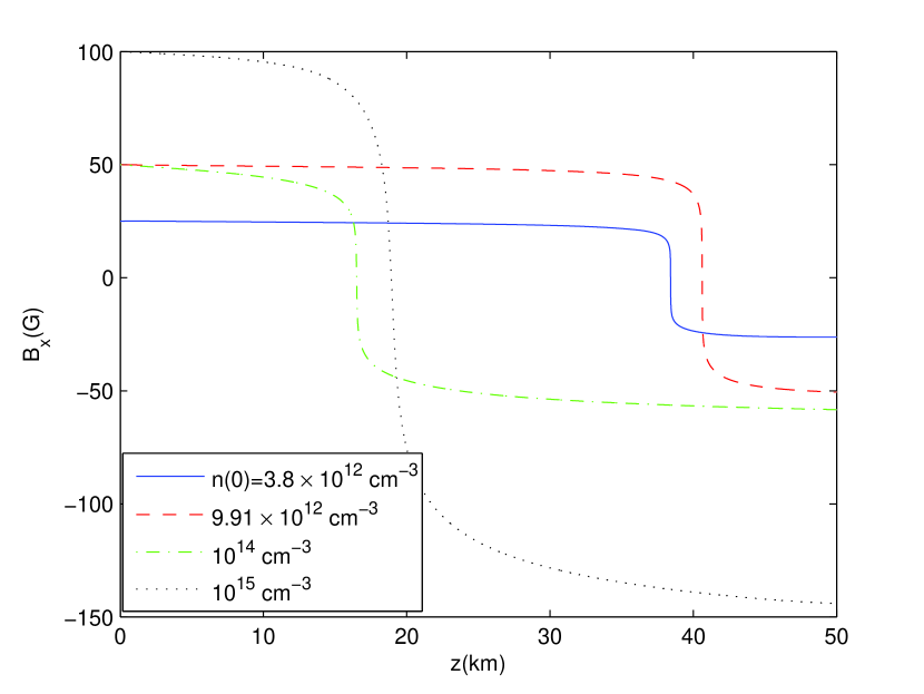
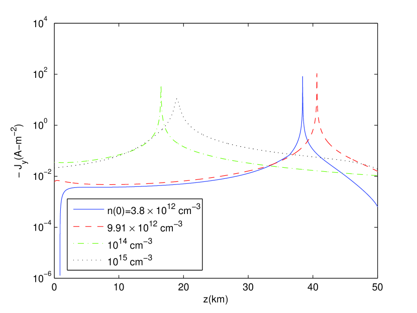
Figure 1: Magnetic field vs. height (left), current density vs. height (right).

Figure 1 shows $B_{x}$ (left panel) and $J_{y}$ (right panel) vs. height for the four solutions. The profiles of $B_{x}$ are close to Harris sheet profiles. There is nothing deliberately built into the model or its inputs to make $B_{x}$ have these profiles.

Not all solutions to the model contain current sheets. Smooth solutions for chromospheric atmospheres extending over a 260 km height range that do not contain current sheets are also found, but not presented here. These atmospheres are weakly heated and weakly radiating compared to the current sheet solutions, and to the energy requirements of the chromosphere.

4.2 Length Scales, Radiative Emission Rate, and Required Numerical Resolution

From the Ohm’s law equation (5) the resistive diffusivity is $c^{2}(1+\Gamma)\eta/(4\pi)$. Dividing this by $V_{z}$ gives the resistive length scale

$$L_{r}=\frac{c^{2}(1+\Gamma)\eta}{4\pi V_{z}}.$$ (24)

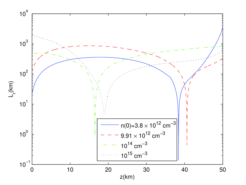
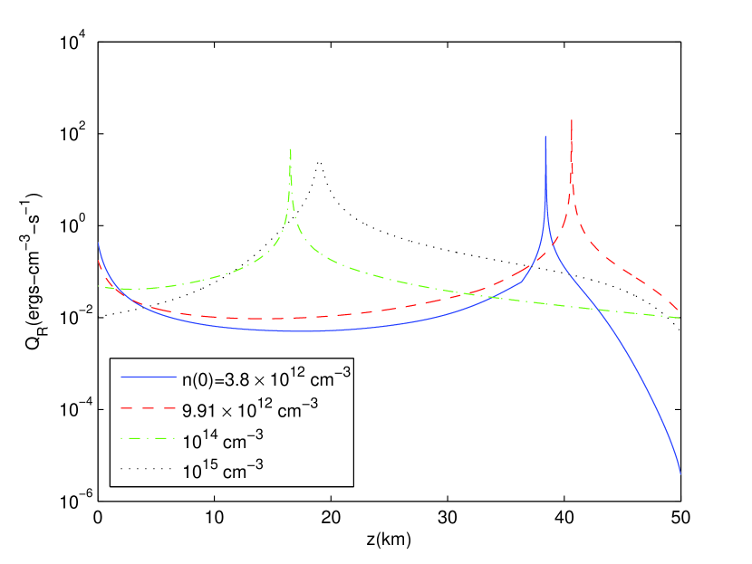
Figure 2: Resistive length scale (equation 24) vs. height (left), radiative cooling rate (equation 12) vs. height (right).

Figure 2 (left panel) shows $L_{r}$ vs. height for each solution. It is found that $L_{r}$ characterizes the thickness of the current sheets in that essentially all of the radiative emission is from a region with a thickness equal to a few times the minimum value of $L_{r}$ for a given sheet. This region is centered around the height at which $Q_{R}$ is a maximum and $L_{r}$ is a minimum.

Figure 2 (right panel) shows $Q_{R}$. The radiative flux $F_{R}$ is the integral of $Q_{R}$ over the height range of the solutions. For the four sheets, in order of increasing $n(0)$, $F_{R}=(0.488,1.55,1.03,4.45)\times 10^{6}$ ergs-cm^-2-s^-1. Although the maximum peak values of $Q_{R}$ occur for the smallest values of $n(0)$, the overall trend is for $F_{R}$ to increase as $n(0)$ increases. This is due to the increase of $L_{r}$ as $n(0)$ increases. Although the peak values of $Q_{R}$ tend to decrease with increasing $n(0)$, $L_{r}$ increases enough with increasing $n(0)$ to make $F_{R}$ follow the same trend. The sheets are strongly radiating in that each sheet radiates $\sim 5-45\%$ of the observed chromospheric radiative loss, with the percentage increasing with increasing $n(0)$, interpreted as decreasing height in the chromosphere.

Magnification of the profiles for $Q_{R}$ show that essentially all of $F_{R}$ is due to emission from a region with a thickness $\sim 2-4$ times the minimum value of $L_{r}$ for a given solution. These regions are centered around the height where $Q_{R}$ is a maximum. These thicknesses are $\sim 0.5,0.7,2.7$, and $13$ km. It is also found that for the four sheets $\sim 50,50,40$, and $70\%$ of $F_{R}$ is due to emission from a sub-region 10 times thinner.

The sheets are fully resolved since the minimum allowed step size of the adaptive step code used to solve equations (15)-(21) is many orders of magnitude smaller than the smallest values of $L_{r}$.

These results suggest that simulations and observations need a resolution $\sim 5-100$ m to accurately resolve, and compute the emission from strongly radiating current sheets in the most strongly radiating regions of the chromosphere.

4.3. Temperature, Ionization, Density, and Pressure

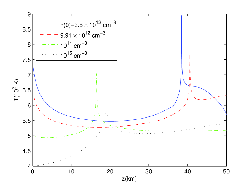
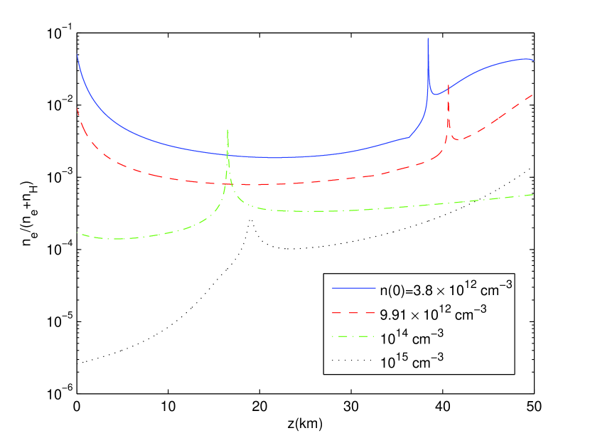
Figure 3: Temperature vs. height (left), ionization fraction vs. height (right).

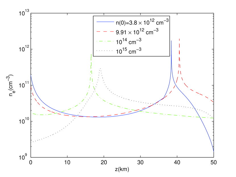
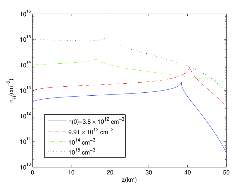
Figure 4: Electron number density vs height (left), HI number density vs. height (right).

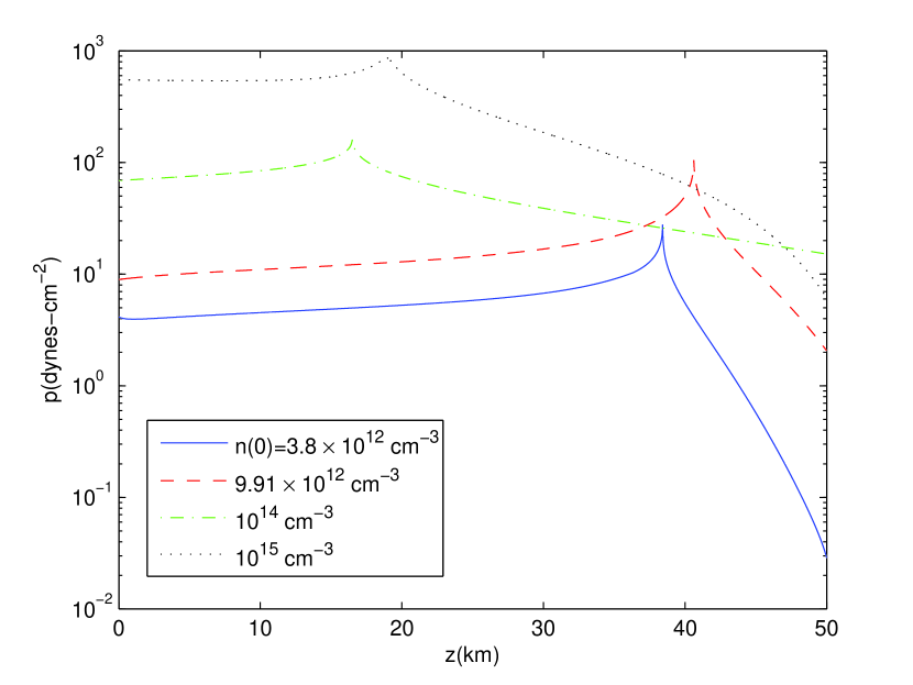
Figure 5: Pressure vs. height.

Figures 3 and 4 show the temperature, ionization fraction $n_{e}/(n_{e}+n_{H})$, and electron and HI densities. Figure 5 shows the pressure. The temperature in the sheets is $\sim 2000-3000$ K higher than in the surrounding plasma. The maximum sheet temperatures are 5800-9000 K. The ionization fraction in the sheets is $\sim 2-20$ times higher than in the surrounding plasma. The maximum values of the ionization fraction are $\sim 2.7\times 10^{-4}-8.4\times 10^{-2}$. The electron density in the sheets is $\sim 10-100$ times higher than in the surrounding plasma. The maximum neutral density in the sheets is $\sim 1.2-3$ times larger than in the surrounding plasma. The pressure experiences a similar increase since the plasma is mainly neutral, and since the maximum temperature in the sheets is $\sim 1.5$ times higher than the temperature in the surrounding plasma.

The results of §§4.1-4.3 show that the current sheet solutions are characterized by plasma conditions believed to exist in the lower and middle chromosphere. As $n(0)$ increases, the conditions within and near the corresponding sheet vary from those characteristic of the middle chromosphere to those characteristic of the lower chromosphere.

The sheets are so strongly radiating that, for increasing $n(0)$, the number of sheets needed to emit the total net radiative flux from the chromosphere is $\sim 20,7,10$, and 2. This result is discussed further in §5 in the context of the constraints that observations place upon the existence and filling factor of such strongly radiating sheets.

4.4. Thermal Energy Balance and Driver of the Radiative Emission

The thermal energy equation (14) may be written symbolically as $Q_{R}=Q_{J}+Q_{c}-Q_{ce}$, which indicates the energy sources that determine the radiative emission. Here $Q_{c}\equiv-p\nabla\cdot{\bf V}=-pV_{z}^{\prime}$ is the compressive heating rate, and $Q_{ce}\equiv\nabla\cdot\left(\left(3p/2+\chi_{H}n_{e}\right){\bf V}\right)=\left(\left(3p/2+\chi_{H}n_{e}\right)V_{z}\right)^{\prime}$ is the heating rate due to the convective energy (ce) flux of thermal and ionization energy, which describes the net flow of this energy into a region.

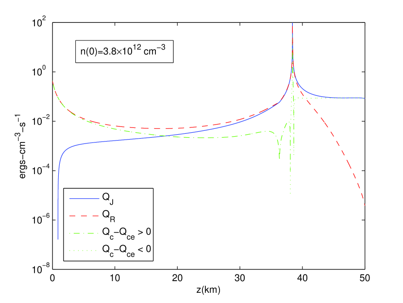
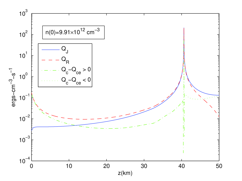
Figure 6: Terms in the thermal energy equation (14) vs. height for the solution with $n(0)=3.8\times 10^{12}$ cm^-3 (left), and for the solution with $n(0)=9.91\times 10^{12}$ cm^-3 (right).

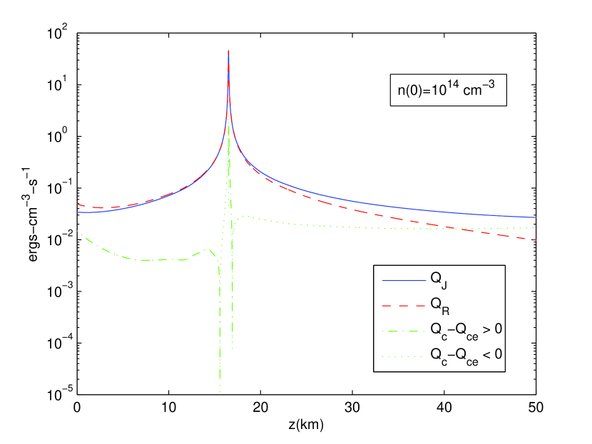
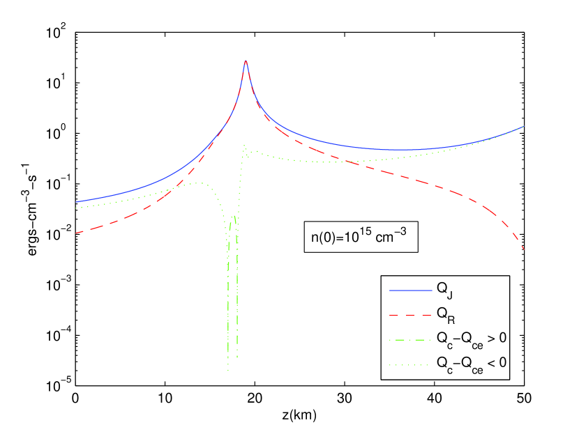
Figure 7: Terms in the thermal energy equation (14) vs. height for the solution with $n(0)=10^{14}$ cm^-3 (left), and for the solution with $n(0)=10^{15}$ cm^-3 (right).

Figures 6 and 7 show $Q_{J},Q_{R}$, and $Q_{c}-Q_{ce}$ for each of the solutions. $Q_{c}-Q_{ce}$ does not make a significant contribution to $F_{R}$, but plays an important role in energy balance outside the sheets where $Q_{R}$ is not significant.

Define the Joule, compressive, and convective energy fluxes $F_{J},F_{c}$, and $F_{ce}$ as the integrals of $Q_{J},Q_{c}$, and $Q_{ce}$ over the height range of a solution. Then $F_{R}=F_{J}+F_{c}-F_{ce}$.

In order of decreasing $n(0)$ the values of these fluxes for each of the four sheets, in units of $10^{6}$ ergs-cm^-2-s^-1, are $(F_{R},F_{J},F_{c},F_{ce})=$$(4.4507,5.9742,-1.3915,-0.13206)$, $(1.0253,1.0845,-0.0561,$ $-0.00311)$, $(1.5499,1.6035,-0.0444,-0.00914)$, $(0.4875,0.5560,$ $-0.0786,0.00999)$.

In the same order, $F_{J}/F_{R}=(1.34,1.06,1.04,1.14)$, so Joule heating is more than sufficient to balance radiative cooling. The excess is balanced mainly by the negative contribution of $F_{c}$.

Joule heating is the primary source of the thermal energy that drives the radiative emission. As discussed in the next section, the primary driver of $F_{R}$ is the static electric field $E_{y}$, and most of $F_{R}$ is due to proton Pedersen current dissipation.

4.5. Driver and Components of the Joule Heating Rate

The Joule heating rate $Q_{J}=J_{y}(E_{y}+V_{z}B_{x}/c)=Q_{P}+Q_{S}+Q_{T}$. The first equality shows that $Q_{J}$ is driven by the CM electric field, which is the sum of the static electric field $E_{y}$, and the convection electric field $V_{z}B_{x}/c$. The relative importance of these two drivers is discussed in §4.5.1. The second equality shows that $Q_{J}$ has three components, due to different physical processes. The contributions of each one is discussed in §4.5.2, and the related magnetization induced resistivity is discussed in §4.5.3.

4.5.1. Convection vs. Static Electric Field Driven Joule Heating

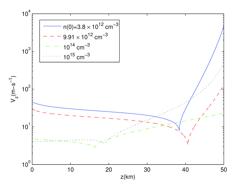
Figure 8: Center of mass flow velocity vs. height.

Let $Q_{J,m}$ be the maximum value of $Q_{J}$ for a given sheet. It is found that for all solutions the ratio $|V_{z}B_{x}/cE_{y}|\sim 10^{-4}-10^{-1}$ in the region where $Q_{J}\geq 10^{-2}Q_{J,m}$, and is $\sim 10^{-3}-10^{-1}$ in the region where $Q_{J}\geq 10^{-1}Q_{J,m}$. For all sheets, the smallest values of the ratio are in the regions where $Q_{J}$ is a maximum. Then it is $E_{y}$ that directly drives $Q_{J}$. Part of the reason for this is the relative smallness of $V_{z}$. As shown in figure 8, $V_{z}\sim 3-10$ m-s^-1 in the regions that emit essentially all of $F_{R}$. This is 2-3 orders of magnitude smaller than characteristic sound and MHD wave speeds, and expected field-aligned flow speeds in the lower and middle chromosphere.

4.5.2. Components of $Q_{J}$

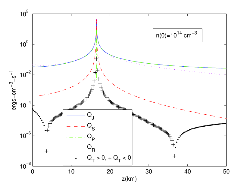
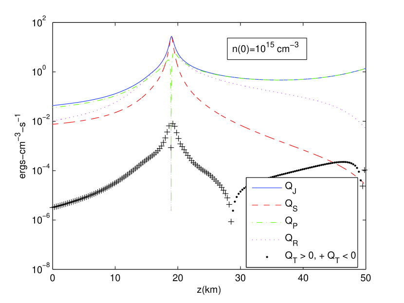
Figure 10: Joule heating rate and its components, together with the radiative cooling rate vs. height for the solution with $n(0)=10^{14}$ cm^-3 (left), and for the solution with $n(0)=10^{15}$ cm^-3 (right).

Figures 9 and 10 show the components of $Q_{J}$ along with $Q_{R}$ for comparison. Define the Spitzer, Pedersen, and thermoelectric heat fluxes $F_{S},F_{P}$, and $F_{T}$ as the integrals of $Q_{S},Q_{P}$, and $Q_{T}$ over $z$. Then $F_{J}=F_{S}+F_{P}+F_{T}.$

In order of decreasing $n(0)$ the values of these fluxes for each of the four sheets, in units of $10^{6}$ ergs-cm^-2-s^-1, are $(F_{R},F_{J},F_{P},F_{S},F_{T})=$ $(4.451,5.974,3.694,2.282,-0.0012)$, $(1.025,1.085,0.779,$ $0.316,-0.0105)$, $(1.55,1.604,1.209,0.486,-0.0913)$, $(0.488,0.556,0.502,$ $0.153,-0.099)$.

In the same order, the fraction of the resistive heating due to Pedersen current dissipation is $F_{P}/(F_{P}+F_{S})=(0.6181,0.7113,0.7131,0.7662)$. This shows that Pedersen current dissipation makes the dominant positive contribution to $F_{J}$ ($F_{T}$ makes a negative contribution), and hence is the main source of the thermal energy that drives radiative loss. The variation of $F_{P}/(F_{P}+F_{S})$ with $n(0)$ suggests that Pedersen current dissipation becomes increasingly dominant with increasing height in the chromosphere, consistent with the expected increase of the magnetization induced resistivity $\Gamma\eta$ with increasing height.

$F_{T}$ makes a small to moderate negative contribution to $F_{J}$ that in magnitude is $\sim 0.02-15\%$ of the positive contribution of $F_{P}+F_{S}$ to $F_{J}$. This thermoelectric cooling effect is largest in the lowest density current sheet. This sheet has the largest temperature gradient.

4.5.3. Magnetization Induced Resistivity

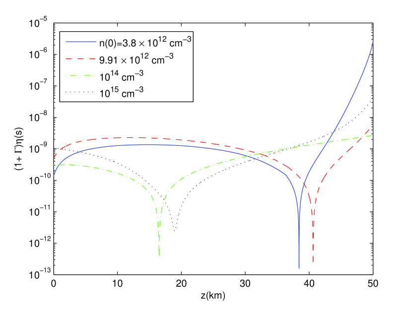
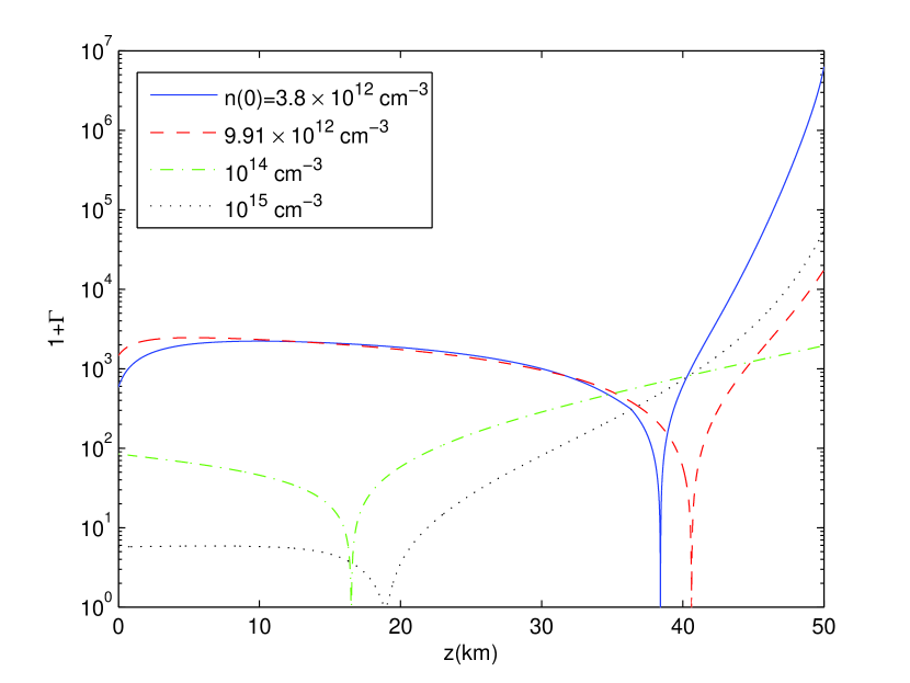
Figure 11: Total resistivity vs. height (left), and ratio of total resistivity to Spitzer resistivity vs. height. This ratio is the magnetization factor + 1 (right).

The total resistivity $(1+\Gamma)\eta$, and the amplification factor $1+\Gamma$ are shown in figure 11. In the thin regions that emit almost all of $F_{R}$, the resistivity decreases by 2-3 orders of magnitude from the exterior to the interior of these regions. Since $\rho_{H}/\rho\sim 1$, and $\Gamma=(\rho_{H}/\rho)^{2}M_{e}M_{p}$, the figure shows that this variation is entirely due to the decrease in magnetization. As the neutral sheet is approached $1+\Gamma\rightarrow 1$ since the magnetization factor $M_{e}M_{p}$ tends to zero. Since, as indicated in §4.5.2, $Q_{P}(=\Gamma\eta J^{2})$ comprises $62-77\%$ of the positive contribution to $Q_{J}$, it follows that the magnetization induced resistivity $\Gamma\eta$ plays a major role in generating $Q_{J}$, which drives the radiative loss. If $\Gamma$ is set equal to zero, the current sheet solutions presented here do not exist.

4.6. Total Energy Conservation and Net Energy Fluxes

Denote the net enthalpy, bulk kinetic energy, gravitational potential energy, ionization energy, and Poynting fluxes into the slab $0\leq z\leq H=50$ km by $F_{H},F_{KE},F_{g},F_{ion}$, and $S_{z}$. They are respectively the differences between the values of $5pV_{z}/2,\rho V_{z}^{3}/2,-\rho gR_{\odot}V_{z},\chi_{H}n_{e}V_{z}$, and $-cE_{y}B_{x}/4\pi$ at $z=0$ and $z=H$, where $R_{\odot}$ is the solar radius. For example $F_{H}=5(p(0)V_{z}(0)-p(H)V_{z}(H))/2$. Here $F_{g}=0$ since $\rho V_{z}$ is constant. Define the total non-radiative flux $F_{NR}=F_{H}+F_{KE}+F_{ion}+S_{z}$.

Combining the momentum and thermal energy equations with Poynting’s theorem gives the total energy equation. It states that the divergence of the total energy flux is zero. Integrating this equation over the slab gives $F_{NR}=F_{R}$.

For the four solutions in order of increasing $n(0)$, and in units of $10^{6}$ ergs-cm^-2-s^-1, the net fluxes are as follows: $(F_{H},F_{KE},F_{ion},S_{z},F_{R})=$ $(-0.1924,-0.7906\times 10^{-3},-1.2571\times 10^{-2},4.7572,4.4507)$, $(-0.309\times 10^{-2},-2\times 10^{-7},-0.427\times 10^{-3},1.043,1.0253)$, $(1.64\times 10^{-3},-3.8\times 10^{-6},-0.3264\times 10^{-2},1.5601,1.5499)$, and $(-0.01183,-3.2161\times 10^{-3},0.4383\times 10^{-2},0.4816,0.4875)$. Since $S_{z}\sim 20-1000$ times larger than any other non-radiative flux, it is essentially the net upward Poynting flux into the slab that drives the heating and corresponding radiative loss.

For the four solutions in order of increasing $n(0)$, $F_{NR}$ equals $F_{R}$ with a relative numerical error of $2.26,1.38,0.55$, and $1.38\%$. This is a check on the accuracy of the numerical solution.

5. Discussion and Conclusions

The current sheet solutions presented here represent the first, first principles theoretical proof of the existence of radiating current sheets under chromospheric conditions, based on a self-consistent model that includes reasonably realistic descriptions of anisotropic electrical conduction and thermoelectric effects, and NLTE ionization and radiative cooling. The existence of these solutions suggests the existence of sub-resolution, horizontal current sheets in the chromosphere that are sites of strong Joule heating driven radiative emission in that no more than a few tens of the sheets collectively emit the total radiation flux from the chromosphere.

Current observations cannot rule out the existence of such strongly radiating current sheets. As indicated in §4.2, the model predicts that essentially all radiative emission from the sheets comes from regions with thicknesses $\lesssim 1-10$ km. A spatial resolution $\lesssim$ a few km would be necessary to image individual sheets seen edge-on, and a resolution $\sim 10-100$ times smaller would be necessary to accurately determine the properties of the sheets. The current best images of chromospheric plasma have a much lower resolution $\sim 100$ km (e.g. van Noort & Rouppe van der Voort 2006). But for random viewing angles most such sheets would be seen as much larger sheet structures with dimensions unspecified in the 1.5 D model used here.

Even if such strongly radiating sheets exist, they cannot be the only significant source of chromospheric heating, for the following reason. Their small thickness combined with the small number of sheets needed to balance the chromospheric net radiative loss imply the filling factor of such a collection of sheets would be so small that their collective emission would be more inhomogeneous than observations of chromospheric emission indicate. Given the complexity of the real chromosphere relative to the model used here, the current sheet solutions presented here are broadly interpreted as evidence that significant chromospheric heating occurs in current sheets with a range of emission rates and filling factors .

The existence of the current sheet solutions presented here proves that the MHD model combined with collision dominated transport and NLTE ionization and radiative cooling contains the essential physics for current sheet formation under chromospheric conditions. The current sheet solutions presented here arise spontaneously as a result of the intrinsic transport physics of the model in that there is no a priori specification of solutions to the model to cause it to generate solutions of this or any other type. These current sheets are not of Sweet-Parker type since the only component of the flow velocity with a gradient is in the direction perpendicular to the sheets, and since the mass flux normal to the sheet is constant.

The horizontal current sheets modeled here might form as a result of magnetic bipoles rising into the chromosphere as their footpoints separate, creating a region of horizontal magnetic field that may form a current sheet as it is forced into an overlying region with a magnetic field having a horizontal component of opposite magnetic polarity. Since this bipole emergence and rising process occurs continually over the entire surface of the Sun, it might be an important quasi-steady state driver of chromospheric heating.

The Joule heating rate $Q_{J}$ that drives the radiative loss in the current sheets is mainly due to proton Pedersen current dissipation, but electron current dissipation makes a significant contribution due to it being the dominant heating mechanism near the neutral sheet where the plasma is weakly magnetized. It is the absence of a guide magnetic field (i.e. $B_{z}=0$) that causes the magnetization to go to zero at the neutral sheet, causing heating by electron current dissipation determined by the Spitzer resistivity $\eta$ to dominate the heating rate near the neutral sheet. Introducing a guide field strong enough to maintain a state of strong magnetization $(\mbox{i.e.}\;M_{e}M_{p}\gg 1)$ throughout the current sheet would cause $Q_{J}$ to be essentially entirely due to proton Pedersen current dissipation. Introducing a nonzero guide field significantly complicates the model, mainly by increasing the dimensionality of the input parameter space from five to nine. This is discussed in §6.2.

The radiative cooling rate $Q_{R}$, and the degree of ionization are exponentially sensitive functions of $T$, as shown by the ionization and radiative cooling rate equations (9) and (12). Since $T$ is largely determined by $Q_{J}(\sim(1+\Gamma)\eta J_{\perp}^{2})$, it follows that $Q_{R}$ and the degree of ionization are exponentially sensitive functions of the resistivity $(1+\Gamma)\eta$, especially its magnetization induced component $\Gamma\eta$ that gives rise to most of the thermal energy that drives $Q_{R}$. This is an example of why it is necessary to accurately model and numerically resolve transport processes to accurately predict radiative loss in the atmosphere. This argument applies to all potential drivers of chromospheric and coronal heating.

Since most of the heating in the current sheet solutions is due to Pedersen current dissipation, these solutions provide yet another example of how Pedersen current dissipation, in this case driven by what is viewed as a quasi-static induction electric field, can be an important chromospheric heating mechanism. There is a long standing proposition that Pedersen current dissipation is the main chromospheric heating mechanism, causing and maintaining the chromospheric temperature inversion. This proposition is discussed in §6.3.

6. Further Discussion

6.1. Determining the Input Parameters

The input parameter space for the model presented here is five dimensional. There does not appear to be any way to know a priori what sets of input parameter values lead to physically reasonable solutions. After choosing values for $p(0),B_{x}(0)$, and $T(0)$ based on current knowledge of chromospheric conditions, the following three heuristic guidelines are used to constrain the search for $E_{y}$ and $V_{z}(0)$, resulting in the discovery of the current sheet solutions presented here, and a set of solutions that do not contain current sheets:

1. If $B_{x}(0)>0(<0)$, a necessary condition for the solution to contain a current sheet is that the constant field $E_{y}$ be $<0(>0)$. The reason is that this is the condition for the vertical Poynting flux to point into the current sheet on both sides. This ensures that electromagnetic energy flows into the sheet to provide the energy for the Joule heating that drives radiative emission and ionization.

2. Although $E_{y}$ is constant in the model, it is assumed that it represents a quasi-static field that is essentially constant over an observed characteristic period $t_{c}\sim 600$ s of Doppler intensity oscillations in the chromospheric network (Lites, Rutten & Kalkofen 1993: the full range of observed periods is $\sim 5-20$ min). The $x$ component of Faraday’s law gives $t_{c}|\dot{B_{x}}|\sim c|E_{y}|t_{c}/L$, where $\dot{B_{x}}\equiv\partial B_{x}/\partial t$, and $L$ is the scale height of $E_{y}$. It is required that $L\gg$ the height range of the solutions to the model since $E_{y}$ is assumed constant over this range. It is also required that $t_{c}|\dot{B_{x}}|\ll B_{x}(0)$ in order that the model assumption $\dot{B_{x}}=0$ be justified. Choose $L$ to be twice the ideal gas pressure scale height for $T=7000$ K. Then $L=422.2$ km, which is $\gg$ the 50 km height range over which the solutions are generated. The magnetic field variation $t_{c}|\dot{B_{x}}|$ is estimated as follows. Observed temporal variations in the intensity of the emission from the lower chromospheric network are typically $\sim 20\%$ (Banerjee, Doyle & O’Shea 1999). It is assumed this emission is mainly due to the Pedersen current dissipation rate $\eta\Gamma J_{\perp}^{2}$. This scales with magnetic field strength $B$ as $B^{4}$, where a factor $B^{2}$ comes from the magnetization induced resistivity factor $\Gamma$, and a factor $B^{2}$ comes from $J_{\perp}^{2}$. The fractional change in intensity during the time $t_{c}$ is then assumed to be $\sim(t_{c}/B^{4})\partial B^{4}/\partial t=4t_{c}\dot{B}/B$. Setting this equal to $20\%$ gives $t_{c}\dot{B}/B\sim 0.05$. Based on this estimate choose $t_{c}|\dot{B_{x}}|\sim 0.05B_{x}(0)$. Then the preceding Faraday law estimate for $|E_{y}|$ gives $|E_{y}|\sim 0.05B_{x}(0)L/ct_{c}\sim 3.52\times 10^{-3}B_{x}(0)$ V-m^-1. Then for $B_{x}(0)=25-100$ G, $|E_{y}|\sim 0.09-0.35$ V-m^-1, which is, remarkably and without our prior knowledge, close to the values of $0.12-0.25$ V-m^-1 found for the current sheet solutions.

3. Given the preceding estimate of $E_{y}$, an estimate for $V_{z}(0)$ is obtained by assuming there is no significant Joule heating at the lower boundary point $z=0$, in which case the Ohm’s law is approximately the ideal MHD Ohm’s law, giving $V_{z}(0)\sim-cE_{y}/B_{x}(0)\sim-0.05L/t_{c}\sim 35.2$ m-s^-1, using the preceding estimate of $E_{y}$. This value is comparable to the values of $4-46$ m-s^-1 found for the current sheet solutions.

These guidelines approximately define the region of the input space where the search for solutions was performed, and where current sheet solutions were found to exist. No solutions were found with $V_{z}(0)=0$ or $E_{y}=0$.

6.2. Including a Guide Magnetic Field

The constant guide field $B_{z}$ is set equal to zero to simplify the model. If $B_{z}\neq 0$ the model becomes significantly more complicated in the following way. If $B_{z}=0$, the $x$ component of the Ohm’s law reduces to $E_{x}=0$, consistent with the fact that $\nabla\times{\bf E}=0$ implies that $E_{x}$ is constant. If $B_{z}\neq 0$, the $x$ component of the Ohm’s law becomes an additional differential equation of the model. Then the model is over determined unless it is assumed that $B_{y}\neq 0$. If $B_{y}\neq 0$, it follows from the $x$ and $y$ components of the momentum equation that $V_{x}$ and $V_{y}$ are not constant. These components of the momentum equation can be analytically integrated to obtain $V_{x}(z)$ and $V_{y}(z)$ in terms of $B_{x},B_{y},B_{z}$, and boundary conditions at $z=0$. The number of input parameters required to determine the solution increases from five to nine if $B_{z}\neq 0$, since $B_{z},B_{y}(0),V_{x}(0)$, and $V_{y}(0)$ must now be specified. Although a nonzero $B_{z}$ does not directly affect the current density since $B_{z}$ is constant, the fact that $B_{y}\neq 0$ implies that $J_{x}\neq 0$, which directly affects the Joule heating rate. Since there is variation only with respect to $z$, $J_{z}$ remains zero.

$B_{y}$ cannot be a guide field. The reason is as follows. Assume $B_{y}$ is constant. Allow the constant $B_{z}$ to have any value. The $x$ component of the Ohm’s law, which is $E_{x}=0$ for the model used in the paper, is now $E_{x}+(V_{y}B_{z}-V_{z}B_{y})/c=\eta J_{y}(M_{e}B_{z}/B-\Gamma B_{x}B_{y}/B^{2})$, where $E_{x}$ and $V_{y}$ are constant. This $z$ dependent equation is an additional equation that must be satisfied. This equation over-determines the solution to the model, so in general there are no non-trivial solutions. Then a nonzero $B_{y}$ must depend on $z$, and so cannot be a guide field.

A guide field prevents the magnetization, and hence the magnetization induced resistivity $\Gamma\eta$, from decreasing to zero at the neutral sheet. An important question is whether a guide field has a significant effect on the radiative emission flux $F_{R}$. Since $F_{R}$ is driven mainly by resistive heating, which is partly determined by the resistivity $(1+\Gamma)\eta$, and since the presence of a guide field increases $\Gamma$, it is expected that the guide field has a direct effect on $F_{R}$. Although the model outlined in the first paragraph of this section must be solved to obtain a reliable estimate of the effect of a guide field, a simple though crude estimate of the effect of a small guide field on $F_{R}$ is obtained as follows. Modify $\Gamma(\propto B^{2}=B_{x}^{2})$ by replacing $B^{2}_{x}$ by $B^{2}_{x}+(0.1B_{x}(0))^{2}$, where $B_{x}(0)$ is the given boundary value of $B_{x}$. This ad hoc modification mimics the effect on the resistivity of a guide magnetic field that is one order of magnitude smaller than $B_{x}(0)$. Then as the neutral sheet is approached, $\Gamma\rightarrow$ a non-zero value instead of zero. Running the code with this modification leads to a set of current sheets as before, and to corresponding values of $F_{R}$ that differ from those for the solutions discussed in the paper by $(-0.04,-0.11,0.09,-0.007)\%$, in order of increasing number density. These differences are insignificant, and are consistent with the values of $\Gamma$ at the neutral sheets, which are $(0.1564,0.1123,0.0975,0.0245)$. Since $\Gamma\ll 1$, the resistivity in the neighborhood of the neutral sheets is $\sim\eta$, as in the absence of a guide field. Since $\eta$ is mainly a function of $T$, and since $T$ in the neighborhood of the neutral sheets for the modified solutions differs by $\lesssim 4.15\times 10^{-2}\;\%$ from its values for the solutions discussed in the paper, it follows that the value of $\eta$ in this neighborhood does not change. These results suggest that the addition of a guide field that is a factor of 10 or more smaller than the asymptotic value of the field component that generates the current density does not have a significant effect on the emission rate.

6.3. Pedersen Current Dissipation and Chromospheric Heating

Pedersen currents are mainly ion currents that flow along and are driven by ${\bf E}_{CM\perp}\equiv$ ${\bf E}_{\perp}+({\bf V}\times{\bf B})/c$, where ${\bf E}_{\perp}$ is the component of ${\bf E}\perp{\bf B}$ (e.g. Mitchner & Kruger 1973).

Osterbrock (1961), following similar work by Piddington (1956), presents an analysis of damping rates of linear MHD waves in the chromosphere due to charged particle-neutral collisions, and a scalar viscosity, and concludes that damping of these waves is not important for chromospheric heating. Due to observational limitations at that time, Osterbrock (1961) uses magnetic field strengths orders of magnitude smaller than those now known to exist, causing the heating rate due to charged-particle neutral collisions to be under estimated by orders of magnitude. Advances in observations since 1961, combined with the largely complete development of the theory of collision dominated transport in variably ionized plasmas (Braginskii 1965) allowed for the recognition through theoretical modeling that Pedersen current dissipation may be an important chromospheric heating mechanism.

There is a longstanding proposition that Pedersen current dissipation provides essentially all the thermal energy that drives chromospheric radiative emission, and that it is the increase in the magnetization of the plasma with height from the photosphere that triggers the onset of heating by Pedersen current dissipation sufficient to cause and maintain the chromospheric temperature inversion (Goodman 2000, 2004a).

Heating by Pedersen current dissipation is not effective in the weakly ionized, weakly magnetized photosphere because the magnetization induced resistivity $\Gamma\eta(=M_{e}M_{i}(\rho_{H}/\rho)^{2}\eta)<\eta$ due to weak magnetization $(M_{e}M_{i}<1)$, and it is not effective in the strongly ionized, strongly magnetized corona because $\Gamma\ll 1$ due to strong ionization $((\rho_{H}/\rho)^{2}\ll 1)$. This heating mechanism can only be effective in the weakly ionized, strongly magnetized chromosphere, between the photosphere and corona, since it is only there where $\Gamma$ can be orders of magnitude greater than unity, causing the plasma to be highly resistive with respect to the flow of Pedersen currents, allowing for, but not guaranteeing significant resistive heating.

Although $\Gamma\eta$ can take on values orders of magnitude larger than $\eta$ under chromospheric conditions (e.g. figure 11, and references cited in this section), a large resistivity does not by itself imply a significant heating rate. An outstanding question is what are the primary drivers of Pedersen current dissipation in the chromosphere, and are they sufficiently strong to cause significant chromospheric heating? Any process that generates an ${\bf E}_{CM\perp}$ can in principle drive a Pedersen current, and hence some level of heating by Pedersen current dissipation. The initial modeling of driving by convection electric fields, generated by the steady bulk flow of plasma $\perp{\bf B}$ is presented in Goodman (1997a,b), and extended in Goodman (2004b). The initial modeling of driving by linear Alfvén waves is presented in DePontieu & Haerendel (1998) and DePontieu, Martens & Hudson (2001). Their basic model is extended in Goodman (2011) to include the full effects of the inhomogeneous background atmosphere on the waves from the photosphere to the lower corona. The initial modeling of driving by slow magnetoacoustic waves, and of Pedersen current dissipation in the shock layers of fast magnetoacoustic shock waves are presented in Goodman (2000, 2001), and Goodman & Kazeminezhad (2010), respectively.

Much additional work has been done in this area. Overall, the models indicate that, under conditions consistent with current understanding of the chromosphere, Pedersen current dissipation driven by several different drivers can provide all the thermal energy needed to balance the total net radiative loss from the chromosphere. What is needed most to determine the effectiveness of this heating mechanism are calculations of ${\bf J}$ based on observations of ${\bf B}$ in the chromosphere. Calculations of this type have been done for sunspot chromospheres (Socas-Navarro 2005a,b; also see comments on those calculations in §6.1.2 of Goodman (2011)). Such calculations are especially challenging since ${\bf J}(\propto\nabla\times{\bf B})$ involves differences of derivatives of components of ${\bf B}$, so any error in the measurement of ${\bf B}$ is multiply compounded in the calculation of ${\bf J}$.

Appendix A Effectively thin radiation loss function

Radiation loss functions $\Phi(T)$ in units of erg cm³ s^-1, have been computed for decades (e.g., Cox & Tucker 1969). When multiplied by electron and hydrogen number densities, they give the power per unit volume, $P$, radiated by an optically thin plasma, given a set of elemental abundances, when the plasma is at a sufficiently low density that only two-body collisions are important, but high enough so that sufficient time has elapsed to reach ionization equilibrium:

$$P=\Phi(T)n_{e}(n_{H}+n_{p})\ \ {\rm erg~{}cm^{-3}~{}s^{-1}}$$ (A1)

Such functions are widely applied in coronal physics. But we need a radiation loss function for the chromosphere, which is in many transitions far from optically thin. Yet it is possible to approximate the radiation losses exactly in the form of eq. (A1), with some care. Radiative transfer affects the radiation loss rates from the chromosphere in two important ways: first, some of the lines become effectively thick, - in such regions these lines must not contribute significantly to the radiation losses; second, the ionization of hydrogen, which in a hydrogen dominated plasma determines $n_{e}$, $n_{H}$ and $n_{p}$, depends on radiation transport in the hydrogen lines and continua. Both of these can be dealt with following the work of Anderson & Athay (1989) and Athay (1986) respectively.

Anderson & Athay (1989) compute radiation losses in detail, using transfer calculations in the abundant emitting species. They show, in their fig. 9, that the function $f(T)\equiv P(T)/(n_{p}+n_{H})$ varies only by a factor of two in quite different models. Furthermore, it follows the form of $n_{e}/n_{H}$, also plotted by them, in regions where the plasma is partially ionized ($n_{e}\ll n_{H}$), i.e. $n_{p}+n_{H}\approx n_{H}$. This figure then demonstrates that the radiation losses in their chromospheric models are reproduced by better than a factor of two, by a formalism of the form of eq. (A1). This is a case where Nature has been kind: while the chromosphere is a difficult, scattering-dominated regime of radiative transfer, the combination of efficient radiating ions (Fe II, Ca II, Mg II) is such that the effectively thin approximation works. All these species belong to dominant stages of ionization in the chromosphere and the scattering does radically affect each individual ion where it is expected to dominate. The bottom line is that the radiation losses can be computed as effectively thin, i.e. the optically thin approximation can be used.

But there are potential problems with this approach. Athay (1986) examined the effects of the inclusion of H L$\alpha$ to genuinely optically thin conditions, versus those that must exist in the upper regions of the chromosphere. The difference is essentially that, under optically thin conditions, photo-ionization of hydrogen by the Balmer continuum photospheric radiation is negligible, whereas under chromospheric conditions, it is significant. The net result is that, compared with optically thin loss functions, the “L$\alpha$ peak” near $2\times 10^{4}$ K is much reduced, since before L$\alpha$ can be emitted at such temperatures, in optically thicker plasmas such as the chromosphere, the otherwise neutral atoms are ionized by the Balmer radiation field from the $n=2$ levels whose populations are enhanced by the scattering of photons that are optically thick in the line core. The proper solution of this problem requires a nLTE transfer calculation, in which transport of radiation (neglected here) is calculated to yield the global coupling of the source function $S$, mean intensity $J$, and then evaluation of $J-S$. Fortunately, in our calculations the temperatures are low enough that the L$\alpha$ radiation never contributes highly to our solutions.

Another potential problem is that we neglect absorption of radiation in the energy equation. But the sheets we have computed are optically thin to most radiation, so that if the internal plasma temperature of the sheet is above the equivalent radiation temperature of radiation from the surrounding plasma (set for example, by light emitted at a far deeper layer of the atmosphere such as the photosphere), then this is not a serious problem. Given that the temperatures we derive are higher than the photosphere of the Sun, we believe that our calculations are accurate enough. So finally, we computed the function $\Phi(T)$ using the following data sources. For ionization balance, we assume iron, calcium and magnesium, the dominant radiators, are singly ionized through the chromosphere- this is a valid approximation (Vernazza, Avrett & Loeser 1981). Otherwise we use the ionization and recombination coefficients of Arnaud+Rothenflug (1985) and compute two-body recombination rates using the OPACITY project cross sections, which includes dielectronic recombination through the inclusion of the resonances in photoionization cross sections. (Seaton 1987). A comparison of typical recombination rates computed from the OPACITY project and more detailed work (Nahar & Pradhan 1992) is given in Judge (2007, fig 13): the agreement in recombination rate coefficients is within a factor of two. Such uncertainties propagate to uncertainties in the radiation losses from each element which are $\leq$ a factor of two, and at any temperature, more than one ion contributes to the losses.

For each radiating ion, the optically thin radiation losses depend primarily on the inelastic collision rate with electrons. to compute these rates, we have adopted the CHIANTI database of 2006 (Landi et al. 2006), supplemented with Ca II data which are important in the chromosphere. Radiation losses were computed for abundant elements, and the sum of all these losses was fitted to the form of eq. (13). This functional form fails above $1.5\times 10^{4}$K.

.

.

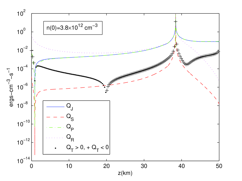
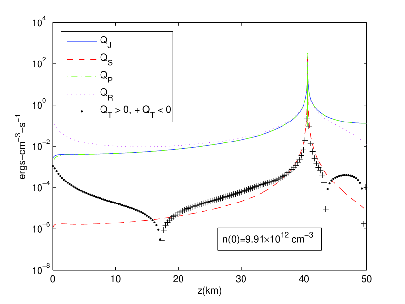
Figure 9: Joule heating rate and its components, together with the radiative cooling rate vs. height for the solution with $n(0)=3.8\times 10^{12}$ cm^-3 (left), and for the solution with $n(0)=9.91\times 10^{12}$ cm^-3 (right).

References

- (1) Anderson, L. & Athay, R. 1989, ApJ, 346, 1010
- (2) Arnaud M. & Rothenflug R. 1985, A&AS, 60, 425
- (3) Athay, R. G. 1986, ApJ, 308, 975
- (4) Banerjee, D., Doyle, J.G. & O’Shea, E. 1999, Solar and Stellar Activity: Similarities and Differences, ASP Conference Series, Vol. 158, C.J. Butler and J.G. Doyle, eds.
- (5) Biskamp, D. 1997, Nonlinear Magnetohydrodynamics, Cambridge Monographs on Plasm Physics (Cambridge University Press)
- (6) Biskamp, D. 2000, Magnetic Reconnection in Plasmas, Cambridge Monographs on Plasm Physics (Cambridge University Press)
- (7) Biskamp, D. 2003, Magnetohydrodynamic Turbulence (Cambridge University Press)
- (8) Boozer, A.H. 2004, Rev. Mod. Phys., 76, 1071
- (9) Boozer, A.H. 2005, Physics of Plasmas, 12, 070706
- (10) Braginskii, S.I., Transport Processes in a Plasma. Reviews of Plasma Physics, edited by Leontovich, M.A., Vol. 1 (Consultants Bureau, New York 1965). p. 205
- (11) Chae, J., Goode, P.R. & Ahn, K. et al. 2010, ApJ, 713, L6
- (12) Cox, D. P. & Tucker, W. H. 1969, ApJ, 157, 1157
- (13) De Pontieu, B. & Haerendel, G. 1998, A&A, 338, 729
- (14) De Pontieu, B., Martens, P.C.H. & Hudson, H.S. 2001, ApJ, 558, 859
- (15) Goodman, M.L. 1997a, A&A, 324, 311
- (16) Goodman, M.L. 1997b, A&A, 325, 341
- (17) Goodman, M.L. 2000, ApJ, 533, 501
- (18) Goodman M.L. 2001, Space Sci. Rev., 95, 79
- (19) Goodman, M.L. 2004a, A&A, 416, 1159
- (20) Goodman, M.L. 2004b, A&A, 424, 691
- (21) Goodman, M. L. & Kazeminezhad, F. 2010 , ApJ, 708, 268
- (22) Goodman, M.L. 2011, ApJ, 735, 45
- (23) Guglielmino, S.F., Zuccarello, F., Romano, P. & Bellot Rubio, L.R. 2008, ApJ, 688, L111
- (24) Hartmann, L. & MacGregor, K.B. 1980, ApJ, 242, 260
- (25) Judge, P.: 2007, THE HAO SPECTRAL DIAGNOSTIC PACKAGE FOR EMITTED RADIATION (haos-diper) Reference Guide (Version 1.0), Technical Report NCAR/TN-473-STR, National Center for Atmospheric Research
- (26) Krall, N.A. & Trivelpiece, A.W. 1986, Principles of Plasma Physics (San Francisco Press)
- (27) Landi, E., Del Zanna, G. & Young, P.R. et al. 2006, ApJS, 162, 261
- (28) Lites, B.W. 2009, Space Sci. Rev., 144, 197
- (29) Lites, B.W., Rutten, R.J. & Kalkofen, W. 1993, ApJ, 414, 345
- (30) Martínez González, M.J. & Bellot Rubio, L.R. 2009, ApJ, 700, 1391
- (31) Mitchner, M. & Kruger, C.H. 1973, Partially Ionized Gases (Wiley, New York)
- (32) Nahar, S. & Pradhan, A. K. 1992, Phys. Rev. Lett., 68, 1488
- (33) Osterbrock, D.E. 1961, ApJ, 134, 347
- (34) Parker, E.N. 1979, Cosmical Magnetic Fields, International Series of Monographs on Physics (Oxford University Press)
- (35) Parker, E.N. 1994, Spontaneous Current Sheets in Magnetic Fields, International Series on Astronomy and Astrophysics (Oxford University Press)
- (36) Petrie, G.J.D. & Patrikeeva, I. 2009, ApJ, 699, 871
- (37) Piddington, J.H. 1956, MNRAS, 116, 314
- (38) Priest, E. & Forbes, T. 2000, Magnetic Reconnection: MHD Theory and Applications (Cambridge University Press)
- (39) Seaton, M. J. 1987, J. Phys. B: At. Mol. Phys., 20, 6363
- (40) Shibata, K., Nakamura, T. & Matsumoto, T. et al. 2007, Science 318, 1591
- (41) Socas-Navarro, H. 2005a, ApJ, 631, L167
- (42) Socas-Navarro, H. 2005b, ApJ, 633, L57
- (43) van Noort, M.J. & Rouppe van der Voort, L.H.M. 2006, ApJ, 648, L67
- Vernazza et al. (1981) Vernazza, J., Avrett, E., and Loeser, R.: 1981, ApJS, 45, 635
- (45) Yamada, M. 2007, Phys. of Plasmas, 14, 058102
- (46) Yamada, M., Kulsrud, R. & Ji, H. 2010, Rev. Mod. Phys., 82, 603
.
.