Impact of approximate oscillation probabilities in the analysis of three neutrino experiments

Abstract

As neutrino oscillation data becomes ever more precise, the use of approximate formulae for the oscillation probabilities ${\mathcal{P}}_{\alpha\beta}$ must be examined to ensure that the approximation is adequate. Here, the oscillation probability ${\mathcal{P}}_{ee}$ is investigated in the context of the Daya Bay experiment; the oscillation probability ${\mathcal{P}}_{\mu\mu}$ is investigated in terms of the T2K disappearance experiment; and the probability ${\mathcal{P}}_{\mu e}$ is investigated in terms of the T2K appearance experiment. Daya Bay requires ${\mathcal{P}}_{ee}$ in vacuum and thus the simple analytic formula negates the need for an approximate formula. However, improved data from T2K will soon become sensitive to the hierarchy, and thus require a more careful treatment of that aspect. For the other cases, we choose an expansion by Akhmedov et al. which systematically includes all terms through second order in $\sin\theta_{13}$ and in $\alpha=:\Delta_{21}/\Delta_{31}$ ($\Delta_{jk}=:m^{2}_{j}-m^{2}_{k}$). For the T2K disappearance experiment the approximation is quite accurate. However, for the T2K appearance experiment the approximate formula is not precise enough for addressing such questions as hierarchy or the existence of CP violation in the lepton sector. We suggest the use of numerical calculations of the oscillation probabilities, which are stable, accurate, and efficient and eliminate the possibility that differences in analyses are emanating from different approximations.

I Introduction

The oscillation of three neutrino flavors can be parameterized in terms of six real independent parameters: three mixing angles $\theta_{jk}$, two mass-squared differences $\Delta_{jk}:=m_{j}^{2}-m_{k}^{2}$, and the Dirac CP phase $\delta_{CP}$. The goal of neutrino oscillation experiments is to measure these parameters with high precision. Broadly, these experiments fall into one of two categories: single-parameter constraint or multi-parameter sensitivity. Through shrewd experimental design or wise choice of baseline or neutrino energy, an experiment can be predominantly sensitive to only one of these parameters. That is, the experiment can cleanly extract the value of a single parameter with little sensitivity to the precise values of the other parameters. As examples, the Daya Bay An et al. (2014) experiment provides a clean measurement of the mixing angle $\theta_{13}$, and long-baseline muon disappearance experiments, like MINOS Adamson et al. and T2K Abe et al. (2013), are able to determine the mass-squared difference $\Delta_{32}$ with minimal knowledge of other parameters.

On the other hand, experiments designed to measure other oscillation properties, like the ordering of the mass eigenstates or the value of the CP phase, are particularly sensitive to the values of the oscillation parameters determined by other experiments. As an example, measurements of electron neutrino appearance in a muon neutrino beam, such as with T2K and NO$\nu$A Jedin (2014), can be used to ascertain the neutrino mass hierarchy or the existence of CP violation, but the extraction of these features relies heavily upon the mixing parameters measured by other experiments. The interdependent sensitivity of these extracted parameters on other parameters requires a careful understanding of how commonly used approximate neutrino oscillation formulae may affect the outcome of an analysis.

Herein, we examine the adequacy of utilizing approximate formulae for the oscillation probabilities in the analysis of neutrino oscillation experimental data. For approximate formulae, we adopt the highly cited perturbative expansion proposed in Ref. Akhmedov et al. (2004), which systematically incorporates all terms of second-order in the small quantities $\sin\theta_{13}$ and the ratio of the mass-squared differences $\alpha:=\Delta_{21}/\Delta_{31}$. To numerically compute the exact oscillation probabilities in matter, we use the method of Ohlsson and Snellman Ohlsson and Snellman (2000). We consider three representative experiments: Daya Bay An et al. (2014), the T2K disappearance experiment Abe et al. (2013), and the T2K appearance experiment Abe et al. (2014a). When evaluating the utility of an approximation, of primary importance is the accuracy of the extracted oscillation parameters, not solely the accuracy of the oscillation probability. Given this, we extend our investigation beyond the usual assessment of deviations between probabilities to deviations between statistical outcomes based on differing probability formulae.

II The Daya Bay Experiment and $\theta_{13}$

In this section, we examine the mixing angle $\theta_{13}$ in the context of the Daya Bay experiment. The exact formula for the vacuum electron neutrino survival probability is

$${\mathcal{P}}_{ee} = 1$$ (1)

$$- \sin^{2}2\theta_{13}\,(c^{2}_{12}\,\sin^{2}\phi_{31}+s^{2}_{12}\,\sin^{2}\phi_{32})$$

$$- c^{4}_{13}\,\sin^{2}2\theta_{12}\,\sin^{2}\phi_{21}\,\,,$$

with $s_{jk}:=\sin\theta_{jk}$, $c_{jk}:=\cos\theta_{jk}$, and $\phi_{jk}:=1.267\,\Delta_{jk}L/E$, where the baseline $L$ is in meters, the neutrino energy $E$ is in MeV, and the mass-squared differences $\Delta_{jk}$ are in eV². Although the exact vacuum oscillation formula is simple and easy to use, we learn some things by investigating its validity.

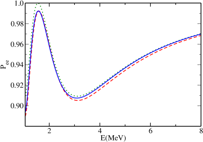
Figure 1: The oscillation probability ${\mathcal{P}}_{ee}$ as a function of $E$ for a baseline of $L=1626$ m. The solid (blue) line represents multiple indistinguishable calculations: the exact vacuum oscillation probability for either hierarchy, the exact oscillation probability through matter of density 2.65 g/cm³, and the $\Delta_{ee}$ approach including the $\phi_{21}$ term from Eq. 1. The dotted (green) curve represents the exact probability minus the last term in Eq. (1). The dashed (red) curve is the result of the approximation of Ref. Akhmedov et al. (2004).

The Daya Bay experiment measures nuclear reactor electron antineutrinos over a baseline of $L=1626$ m, the flux-averaged distance from the reactors to the far detector. It is the dominant experiment in the determination of $\theta_{13}$. In Fig. 1, we use exact and approximate oscillation formulae to plot the survival probability ${\mathcal{P}}_{ee}$ for an energy range relevant to the Daya Bay experiment.

We can check the accuracy of our computer code by comparing its results with the exact oscillation formula Eq. (1) for vacuum oscillations. The numerical calculation reproduces the analytic formula to the accuracy of the computer, for us, fifteen decimal places. The first question is whether the effects of the interactions of the neutrino with the Earth’s matter may be neglected. Utilizing a typical matter density of 2.65 g/cm³, we find that the percent change in ${\mathcal{P}}_{ee}$ caused by the interaction with matter has two peaks, 0.003% at 1.28 MeV and 0.007% at 2.41 MeV. Matter effects are thus negligible. The second question is whether hierarchy can be neglected. Hierarchy refers to the two cases of the mass ordering: normal hierarchy is the situation when the third mass state has a larger mass than the two other states and inverse hierarchy refers to the case when the third mass state has a mass smaller than the masses of the two other states. We move from the normal to the inverse hierarchy via the map $\Delta_{31}\mapsto-\Delta_{31}+\Delta_{21}$. Changing from normal to inverse hierarchy changes ${\mathcal{P}}_{ee}$ by 0.32% at 2.00 MeV and by 0.12% at 4.73 MeV. We here adopt a convention that if the calculation is better than one percent accurate, it is acceptable. Thus neglecting matter and hierarchy effects is acceptable when considering the oscillation probability. The solid (blue) curve in Fig. 1 represents the vacuum results, the inclusion of matter effects, and the results for either hierarchy.

The dotted (green) curve is the result of omitting the small $\phi_{21}$ term in Eq. (1), assuming normal hierarchy and vacuum oscillations. Historically, this term would be referred to as a subdominant effect. This produces maxima in the percent error of 0.05% at 6.09 MeV and 0.8% at 1.80 MeV, just above the peak. At the peak, the muon interaction rate has become so small that this term has little effect. Although it could be ignored, there is no reason to do so.

The approximate formula for the vacuum electron neutrino survival probability from Ref. Akhmedov et al. (2004) is

$${\mathcal{P}}_{ee}=1-4s^{2}_{13}\sin^{2}\phi_{31}-\alpha^{2}\phi_{31}^{2}\sin^{2}2\theta_{12},$$ (2)

valid to second order in both $\sin\theta_{13}$ and $\alpha$. This produces the dashed (red) curve in Fig. 1. The peak percent difference for this approximation from the exact probability is 0.1% at an energy of 1.80 MeV (near the peak) and 0.3% at 3.76 MeV.

We also examine an approximation used by the Daya Bay collaboration. In this approximation, the oscillations driven by $\Delta_{31}$ and $\Delta_{32}$ are replaced by a single oscillation driven by the mass-squared difference $\Delta_{ee}$ Minakata et al. (2006). This effective mass-squared difference $\Delta_{ee}$ is determined by requiring that the exact and approximate oscillation minima are equal. The result is

$$\Delta_{ee}=c^{2}_{12}\,\Delta_{31}+s^{2}_{12}\,\Delta_{32}\,\,.$$ (3)

The $\sin^{2}\phi_{3j}$ terms in Eq. (1) are averaged by a weighting of $c^{2}_{12}$ and $s^{2}_{12}$. The approximation, Eq. (2), simply transfers this weighted averaging to the mass-squared differences, $\Delta_{3j}$. The difference from the exact result is everywhere less than 0.02%, a very good approximation, and this result is also depicted by the blue curve in Fig. 1.

It is not the accuracy of the oscillation probability that determines whether an approximation is adequate; rather, the ability to extract accurate oscillation parameters from data is the bottom line in determining an approximation’s utility. Thus, in our analysis of the Daya Bay experiment, we compare the extracted values for $\theta_{13}$ that result from the various exact and approximate oscillation formulae. In this analysis, we fix the mixing parameters to their measured values Beringer et al. (2012): $\theta_{12}=0.557$, $\Delta_{21}=7.5\times 10^{-5}$ eV²; and we consider maximal mixing for the atmospheric angle: $\theta_{23}=0.7845$ Adamson et al. (2011); Hosaka et al. (2006). For the larger mass-squared difference, we set $\Delta_{32}=2.54\times 10^{-3}$ eV², the value obtained by Daya Bay for normal hierarchy, so as to make our analysis directly comparable to the Daya Bay analysis.

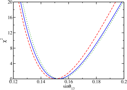
Figure 2: $\Delta\chi^{2}$ versus $\sin\theta_{13}$ for the Daya Bay experiment. The solid (blue) curve is the result of an analysis utilizing the exact oscillation probability, the dashed (red) curve uses the formula from Eq. (2), while the dotted (green) curve uses the exact oscillation probability, neglecting the $\Delta_{21}$ term.

In Fig. 2 we depict $\Delta\chi^{2}$ versus $\sin\theta_{13}$ for our analysis of the Daya Bay experiment. The experimentalists find $\sin^{2}2\,\theta_{13}=0.090^{+0.009}_{-0.008}$ (one sigma errors) An et al. (2014); we find the same result. The color code is the same as for Fig. 1. The solid (blue) curve represents several indistinguishable results achieved by using: the exact expression, either hierarchy, with or without matter effects, or the use of $\Delta_{ee}$ (with the $\phi_{21}$ oscillation term included). The dashed (red) curve employs the approximation in Eq. (2) and the dotted (green) curve employs the exact probability neglecting the $\phi_{21}$ oscillation term. The differences in the three $\Delta\chi^{2}$ curves might seem large for probabilities that differ by tenths of a percent. But the parameter of interest, $\theta_{13}$, is not determined by ${\mathcal{P}}_{ee}$, but rather by $\Delta\mathcal{P}=:1-{\mathcal{P}}_{ee}$. Since $\Delta\mathcal{P}$ peaks at around seven percent, the error for this quantity is larger in percent than the error in ${\mathcal{P}}_{ee}$ itself. From this result, we consider the use of the approximation from Ref. Akhmedov et al. (2004) or dropping the last term in Eq. (1) to be inadequate.

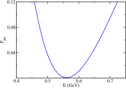
Figure 3: The oscillation probability ${\mathcal{P}}_{\mu\mu}$ versus energy for energies near the oscillation minimum for the T2K experiment with $L=295$ km.

III The T2K $\nu_{\mu}$ disappearance experiment and $\Delta_{32}$

The long-baseline muon disappearance experiments, MINOS Adamson et al. and T2K Abe et al. (2014a), and the Super-K atmospheric experiment Hosaka et al. (2006) yield clean measurements of the mass-squared difference $\Delta_{32}$. We will focus upon the T2K experiment as it is poised to surpass MINOS’ precision in the determination of $\Delta_{32}$ with its next data release. In the T2K experiment, a beam of muon neutrinos travels over a long baseline through the Earth with an, assumed constant, density of 2.6 g/cm³. In Fig. 3 we depict the oscillation probability ${\mathcal{P}}_{\mu\mu}$ as a function of energy in the region near the minimum of the oscillation probability for the T2K experiment assuming a fixed baseline of 295 km. We focus on the minimum of the oscillation probability because we expect to find the differences between the exact and approximate oscillation formulae to be most significant and visible here. In the Figure, the curve represents the oscillation probability using the exact numerical calculation for vacuum oscillations, assuming normal hierarchy. The effects of matter or hierarchy are not sufficiently significant to be visible on this graph. For the inverse hierarchy, there is a 10% change in the probability at the minimum of $\mathcal{P}_{\mu\mu}$, corresponding to an absolute change of only $6\times 10^{-5}$. At higher energies, there is a 0.4% change. Matter results in a 20% change at the minimum, corresponding to an absolute change of $1.5\times 10^{-4}$. At higher energies there is only a 0.02% change.

From Ref. Akhmedov et al. (2004), the approximate formula for the vacuum $\nu_{\mu}$ survival probability, ${\mathcal{P}}_{\mu\mu}$, is:

$${\mathcal{P}}_{\mu\mu} = 1-\sin^{2}2\theta_{23}\,\sin^{2}\phi_{31}$$ (4)

$$+ \alpha\,c^{2}_{12}\,\sin^{2}2\theta_{23}\,\,\phi_{31}\,\sin 2\phi_{31}$$

$$- \alpha^{2}\,c^{2}_{23}\sin^{2}2\theta_{12}\,\phi^{2}_{31}$$

$$- \alpha^{2}\,c^{2}_{12}\,\sin^{2}2\theta_{23}\,\phi^{2}_{31}\,(\cos 2\phi_{31}-s_{12}^{2})$$

$$- 4\,s^{2}_{13}\,s^{2}_{23}\,\sin^{2}\phi_{31}$$

$$+ 2\,s^{2}_{13}\,\sin^{2}2\theta_{23}\,\sin^{2}\phi_{31}$$

$$- 2\,\alpha\,s_{13}\,\sin 2\theta_{12}\,\sin 2\theta_{23}\,s_{23}^{2}\,\phi_{31}\,\sin 2\phi_{31}.$$

This is a very good approximation to use for the T2K experiment. Differences between the exact and approximate oscillation probabilities are so small that they are not visible on the graph in Fig. 3. At the minimum of $\mathcal{P}_{\mu\mu}$ the change is 10%, with an absolute change of $6\times 10^{-5}$. At higher energies, the change is 0.4%.

For the T2K Abe et al. (2014a) disappearance experiment, $\Delta\chi^{2}$ versus $\Delta_{32}$ is shown in Fig. 4. We find that all oscillation probabilities yield equivalent results. That is, the curve represents the exact results of our model for normal and inverse hierarchy, either in vacuum or in constant density matter. The curve also represents the results of using the approximate oscillation formula from Ref. Akhmedov et al. (2004). We have checked to see if any of the terms in this formula might be neglected and found that all are needed to maintain an accuracy better than 0.4%, i.e., less than about a half line width on the plots. There are terms which are zero for $\theta_{23}$ set to maximal mixing, but these cannot be neglected if one wants a generally applicable code.

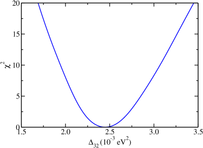
Figure 4: $\Delta\chi^{2}$ versus neutrino mass-squared difference $\Delta_{32}$ for the T2K disappearance experiment. The curve represents the results utilizing the exact probability, either hierarchy, with and without matter effects, and also the use of the approximate oscillation probability given in Eq. (4).

IV The T2K $\nu_{e}$ appearance experiment and hierarchy

The T2K disappearance and Daya Bay experiments are predominantly sensitive to a single parameter, $\Delta_{32}$ and $\theta_{13}$, but with sensitivity to a second parameter, $\theta_{23}$ Abe et al. (2014b) and $\Delta_{32}$, respectively. The $\nu_{\mu}\to\nu_{e}$ appearance probability, ${\mathcal{P}}_{\mu e}$, measured in the T2K appearance experiment is of a different character Abe et al. (2014b). ${\mathcal{P}}_{\mu e}$ is sensitive to matter effects, to the hierarchy of the neutrino oscillations, and to the Dirac CP phase. In order to be able to provide information about these quantities, input is needed from other neutrino oscillation experiments. In what follows, we will assume there is no CP violation and examine the question of hierarchy in the context of the T2K appearance experiment.

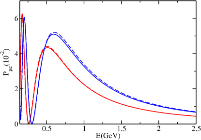
Figure 5: The oscillation probability ${\mathcal{P}}_{\mu e}$ as a function of energy over the energy range appropriate for the T2K appearance experiment. The blue curves employ the normal hierarchy, and red employ the inverse hierarchy. Solid curves use the exact oscillation probability and dashed curves use the approximate probability given in Eq. (5).

As stated earlier, hierarchy refers to the ordering of the mass eigenstates. In particular, is $m_{3}$ less than or greater than $m_{1},m_{2}$? In principle, this can be determined from the T2K appearance data. As shown in Fig. 5, ${\mathcal{P}}_{\mu e}$ is small, only a few percent, in the region where we can presently measure it. This makes getting good statistics difficult. For T2K the detector is located off-axis in order to reduce the background, which also reduces the overall flux, while MINOS Adamson et al. (2013), is on-axis producing a background that is comparable to the signal. The recent T2K results are quite exciting as they are the first measurements that provide clues to the hierarchy question and the existence of CP violation. This is only true because of the relatively large value of $\theta_{13}$ discovered by Daya Bay An et al. (2014) and RENO Ahn et al. (2012).

The approximate oscillation probability for ${\mathcal{P}}_{\mu e}$ from Ref. Akhmedov et al. (2004) is given by

$${\mathcal{P}}_{\mu e} = \alpha^{2}\,c^{2}_{23}\,\sin^{2}2\theta_{12}\,\frac{\sin^{2}(A\,\phi_{31})}{A^{2}}$$ (5)

$$+ 4\,s^{2}_{13}\,s^{2}_{23}\,\frac{\sin^{2}((A-1)\phi_{31})}{(A-1)^{2}}$$

$$+ 2\,\alpha\,s_{13}\,\sin 2\theta_{12}\,\sin 2\theta_{23}\cos\phi_{31}\,$$

$$\times \,\sin(A\phi_{31})\,\frac{\sin((A-1)\phi_{31})}{A(A-1)}\,\,$$

where matter effects are included in the factor $A:=2\,E\,V/\Delta_{31}$ with $V$ the MSW potential in eV.

In Fig. 5 we depict the oscillation probability ${\mathcal{P}}_{\mu e}$ versus energy for the energy range relevant to T2K. The solid curves are exact results, dashed curves the approximation given in Eq. (5). The blue curves are normal hierarchy, the red inverse hierarchy.

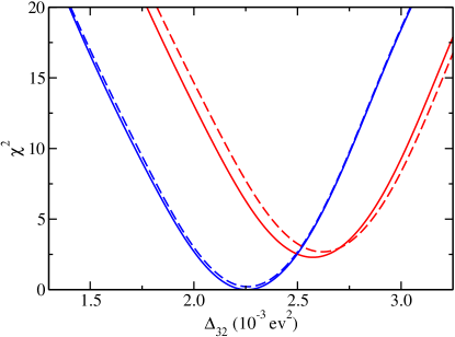
Figure 6: $\Delta\chi^{2}$ versus neutrino mass-squared difference $\Delta_{32}$ for the T2K appearance experiment. The solid curves represent the results of utilizing the exact probability; the dashed curves represent results from utilizing the approximate probability from Eq. (5). The blue curves employ normal hierarchy; the red curves employ inverse hierarchy.

We see the significant hierarchy dependence. The approximate curves are close to the exact curves. For the normal hierarchy, the approximate curve differs from the exact by 3% near the peak, and 4% at higher energies. For the inverse hierarchy, the difference is 2% near the peak and 4% at the higher energies.

In Fig. 6 we show $\Delta\chi^{2}$ versus $\Delta_{32}$ for our analysis of the T2K appearance experiment. The solid curves represent the results utilizing the exact probability; the dashed curves represent results from utilizing the approximate probability from Eq. (5); the blue curves are normal hierarchy; the red curves are inverse hierarchy. For normal hierarchy, the exact curve gives $\Delta_{32}=2.26\pm 0.26\times 10^{-3}$ eV² and the approximate curve gives $2.26\pm 0.25\times 10^{-3}$ eV², a surprisingly good agreement given the difference in the oscillation probabilities. However, for the inverse hierarchy, the exact curve gives $\Delta_{32}=2.57\pm 0.26\times 10^{-3}$ eV² and the approximate curve gives $2.62\pm 0.26\times 10^{-3}$ eV². For the inverse hierarchy, there is a shift in the best fit value for $\Delta_{32}$ of $0.05\times 10^{-3}$ eV² and a shift in the value of $\chi^{2}$ at the minimum of 0.4. This is not large in an absolute sense, but if one wishes to maintain a limit of one percent error on the actual theoretical calculations, this is not acceptable.

V Discussion

We have examined the use of approximate oscillation probabilities for ${\mathcal{P}}_{ee}$ in the context of analyzing the Daya Bay Akhmedov et al. (2004) experiment, ${\mathcal{P}}_{\mu\mu}$ in the context of analyzing the T2K disappearance experiment Abe et al. (2014a), and ${\mathcal{P}}_{\mu e}$ in the context of analyzing the T2K appearance experiment Abe et al. (2014a). Since matter effects for Daya Bay are quite small, the rather simple exact formula for ${\mathcal{P}}_{ee}$ in vacuum can be used. The approximation used by Daya Bay that uses only one mass-squared difference $\Delta_{ee}$ is accurate as long as the $\phi_{21}$ mixing term is included. For the T2K disappearance experiments, the approximation formula of Ref. Akhmedov et al. (2004) is found to be quite accurate, with the vacuum form given in Eq. (4) adequate. All terms in the rather lengthy formula must be included. For the T2K appearance experiment, matter effects must be included. The formula, Eq. (5), is found to give reasonable results for the normal hierarchy but not so for the inverse hierarchy. Based on these results, we find that our investigation raises a number of questions.

First, are these formulae adequate for learning about CP violation? The recent T2K results Abe et al. (2014a) are sensitive to the CP phase and, hence, when combined with reactor data is able to rule out some values of the phase $\delta_{CP}$. Since we are not satisfied by the ability of the approximate formula to discern between hierarchies and since the hierarchy question is deciding between two distinct answers, the approximate formula is certainly not satisfactory to measure the value of the continuous variable $\delta_{CP}$.

The second question is whether or not approximate oscillation probabilities are adequate for the analysis of atmospheric data Hosaka et al. (2006). Atmospheric data are sensitive to both the hierarchy and the CP phase. Can we reliably analyze atmospheric data well enough such that we can extract this information? There exist two published analyses Capozzi et al. (2013); Gonzalez-Garcia et al. (2012) which yield qualitatively different results when addressing the questions of hierarchy and the CP phase. The difference in these results may be due to the use of different approximations for the oscillation probabilities. As it stands, it seems that the approximate probabilities are not adequate for atmospheric data. On the other hand, the atmospheric data has become less significant with the recent, more accurate data from Daya Bay and T2K. The atmospheric data does still affect the final values of $\Delta_{32}$ and $\theta_{23}$, but data coming in from T2K and future data from NO$\nu$A Jedin (2014) will render the contribution from atmospheric data negligible, as Daya Bay has done for $\theta_{13}$.

Third, what is the impact of using various approximate formulae on the consistency of neutrino oscillation analyses? Two points are worth noting. First, different approximations used by different experimental groups applied to data used to constrain the same oscillation parameter, such as the reactor constraints on $\theta_{13}$, may lead to inconsistencies, especially as data becomes more precise. A second, and far more subtle, point is that changing the approximation applied to an updated data set by the same experimental group merits careful interpretation and comparison to previous analyses. The only statistically robust, reproducible analysis is a full exact three neutrino calculation using a numerical code for the case where matter effects are included, or a full exact formula for the case of vacuum. It is not immediately obvious whether or not old and new data releases may appear falsely consistent or inconsistent partly as a result of changing approximations, especially as systematic errors decrease over time. Furthermore, this question reiterates the point discussed above that a possible source of the discrepancy between global analyses is the use of different approximations, particularly for the atmospheric data, which covers a broad range of $L/E$. This leads to one final issue.

For data sets sensitive to many types of oscillation physics, such as matter and hierarchy effects, it is difficult to find or construct reliable approximations that take into account multiple sub-leading effects simultaneously. The danger in using an overly-tailored approximation, designed to constrain only one specific parameter, is the loss of correlations between sub-leading effects which can enrich the final result, much like combining complimentary data sets is more powerful than relying on one data set alone. For data sets which are rich in subtle physics, such as the long-baseline and atmospheric data that are sensitive to matter effects, the CP phase, and the mass ordering, the loss of information resulting from the use of approximate oscillation probabilities has yet to be sufficiently assessed or quantified and, hence, merits continued, careful examination.

VI Conclusions

As neutrino oscillation experiments become increasingly accurate, the need to ensure the robustness and accuracy of analyses of the data becomes more important. Our examination of the variation between analysis outcomes of the same data using different approximate oscillation formulae indicates that the impact of the oscillation formula used on the final results of an analysis should not be underestimated. We stress that our study indicates that the implicit definition of the term “accuracy of an approximate probability” should be expanded to include not only how much it varies from the exact probability but also how robust a statistical analysis of the data is compared to one conducted with the exact probability. The need for continued, thorough pre-assessment of the validity and reliability of approximate oscillation formulae will become increasingly mandatory as systematic errors reach percent level and the signatures of ever more subtle neutrino physics is sought. Already, small discrepancies among global analyses suggest that the data has become precise enough that the “sub-leading effects” picture, which implied the permissible use of expansions that neglect small terms, has outlived its usefulness. For this reason we encourage a shift from the term “sub-leading effects” to “subtle physics,” which implies the need for a more careful and complete treatment of the data.

Fortunately, transitioning from the past era of approximations to the new era of using exact oscillation formulae is simple. To contribute to this effort we will publish the short, concise subroutine implemented here that uses the method of Ref. Ohlsson and Snellman (2000) for calculating oscillation probabilities, including constant matter density and CP effects. The subroutine is stable, efficient, and accurate and thus removes the need to use approximations for the analysis of long-baseline, atmospheric, and solar data. Furthermore, exact vacuum expressions for electron antineutrino disappearance are trivially short and, hence, negate the need to use approximate expressions for analyses of reactor data. The benefit is that progressing to the use of exact oscillation formulae, which is not a computationally burdensome change, will allow future published analyses of neutrino oscillation data to be more robust, more consistent, and more sensitive to the subtle physics of the neutrino mass ordering and CP phase that precision measurement are beginning to make accessible.

References

- An et al. (2014) F. An et al. (Daya Bay Collaboration), Phys. Rev. Lett. 112, 061801 (2014).
- (2) P. Adamson et al. (MINOS Collaboration), arXiv:1403.0867 (2014).
- Abe et al. (2013) K. Abe et al. (T2K Collaboration), Phys. Rev. Lett. 111, 211803 (2013).
- Jedin (2014) F. Jedin (NOvA), J. Phys. Conf. Ser. 490, 012019 (2014).
- Akhmedov et al. (2004) E. K. Akhmedov, R. Johansson, M. Lindner, T. Ohlsson, and T. Schwetz, JHEP 0404, 078 (2004).
- Ohlsson and Snellman (2000) T. Ohlsson and H. Snellman, J. Math. Phys. 41, 2768 (2000).
- Abe et al. (2014a) K. Abe et al. (T2K Collaboration), Phys. Rev. Lett. 112, 061802 (2014a).
- Minakata et al. (2006) H. Minakata, H. Nunokawa, S. J. Parke, and R. Zukanovich Funchal, Phys. Rev. D74, 053008 (2006).
- Beringer et al. (2012) J. Beringer et al. (Particle Data Group), Phys. Rev. D86, 010001 (2012).
- Adamson et al. (2011) P. Adamson et al. (MINOS Collaboration), Phys.Rev. D84, 071103 (2011).
- Hosaka et al. (2006) J. Hosaka et al. (Super-Kamiokande Collaboration), Phys. Rev. D74, 032002 (2006).
- Abe et al. (2014b) K. Abe et al. (T2K Collaboration) (2014b), eprint 1403.1532.
- Adamson et al. (2013) P. Adamson et al. (MINOS Collaboration), Phys. Rev. Lett. 110, 171801 (2013).
- Ahn et al. (2012) J. Ahn et al. (RENO collaboration), Phys. Rev. Lett. 108, 191802 (2012).
- Capozzi et al. (2013) F. Capozzi, G. Fogli, E. Lisi, A. Marrone, D. Montanino, et al. (2013), arXiv:1312.2878.
- Gonzalez-Garcia et al. (2012) M. Gonzalez-Garcia, M. Maltoni, J. Salvado, and T. Schwetz, JHEP 1212, 123 (2012).