Anticipating Activity in Social Media Spikes

Abstract

We propose a novel mathematical model for the activity of microbloggers during an external, event-driven spike. The model leads to a testable prediction of who would become most active if a spike were to take place. This type of information is of great interest to commercial organisations, governments and charities, as it identifies key players who can be targeted with information in real time when the network is most receptive. The model takes account of the fact that dynamic interactions evolve over an underlying, static network that records “who listens to whom.” The model is based on the assumption that, in the case where the entire community has become aware of an external news event, a key driver of activity is the motivation to participate by responding to incoming messages. We test the model on a large scale Twitter conversation concerning the appointment of a UK Premier League football club manager. We also present further results for a Bundesliga football match, a marketing event and a television programme. In each case we find that exploiting the underlying connectivity structure improves the prediction of who will be active during a spike. We also show how the half-life of a spike in activity can be quantified in terms of the network size and the typical response rate.

Keywords network, modelling, microblogging, dynamics, on-line social interaction, spike, Twitter

Lay Summary: Microblogging data offers us the opportunity to understand, and exploit, on-line human behavior. Here, we focus on the task of predicting which users will be influential in the event of an externally-driven spike, such as an unexpected news item. Based on the testable hypothesis that microbloggers generate new content in response to incoming messages, we develop a mathematical model and computational algorithm. The new algorithm combines information about the static user-follower network and the dynamic interaction patterns. We give four Twitter case studies to show that this approach improves our ability to anticipate who would be most active during a spike. This provides a tool for rapid targetting of key users when the network is at its most receptive.

1 Introduction

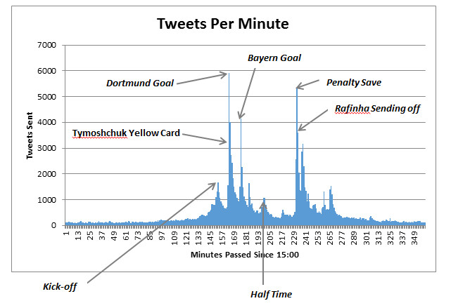
Digital footprints left by our online interactions provide a wealth of information for social scientists and present many new challenges in modelling and computation [16]. In addition to aiding our understanding of how humans interact and make decisions [2], microblogging data offers the prospect of predicting future behavior [8] and engaging in targeted intervention [1]. Commercial organisations, governments and charities are now able to interact with the general public during the course of an online, global conversation, and exploit opportunities to leverage current sentiment. We focus here on the specific case where a rapid spike of activity can be attributed to a high profile event or news item. (For example, a pivotal moment in a sporting event, or an unexpected reality TV voting result.) In Figure 1 we show examples of spikes arising in a European football match: a Bundesliga encounter between Bayern Munich and Borussia Dortmund on May 4th, 2013. The vertical axis records the volume of Twitter activity over each one-minute period. Here, a tweet is deemed to take part in the conversation if it contains one or more specified keywords. The spikes in bandwidth can be attributed to unpredictable external events, including goals and controversial refereeing decisions, as indicated in the figure, with a typical half-life of between ten and twenty minutes. Further Twitter spike examples are illustrated in the next section and in [Supplementary Information]. These dramatic, but short-lived, bursts of interest represent marketing opportunities for suitably agile players, as demonstrated by the cookie company Oreo who produced an effective, and, subsequently award winning, tweet in response to a power failure during Super Bowl XLVII [9].

Several authors have considered how information is passed in the setting of online social media. In [7] the number of followers, Retweets and mentions were used to quantify the influence of Twitter users, with the three measures yielding very different results. Similarly, [14] ranked users by the number of followers and also by Google’s PageRank algorithm. Related work in [18] looked at how network structure affects dynamics of large scale information flow around news stories in Digg and Twitter. In [6] the spread of behavior was examined through artificially constructed, static, social interaction networks, with clustered-lattice structure found to be the most effective in terms of speed and reach. Dynamic analogues of the standard Katz centrality measures were tested on a large scale Twitter data set in [15], and found to be compatible with the rankings produced by social media experts whose job is to identify key targets.

Looking more specifically at temporal patterns within online behavior, [21] used empirical long-time Twitter interaction data to show that the characteristic bursts of activity are compatible with trading volumes of financial securities, and proposed a stochastic point process model to reproduce the distribution of activity levels across time. Person-to-person cascades of information spread have been studied by a number of authors [3, 10, 17, 19, 23, 24]; and we recommend [5] for an overview of models and applications.

Our work differs from previous studies in three main respects. First, rather than looking at the development of cascades within a community (for example the rise of a viral video) we focus on the “event-driven, full attention span” setting where the relevant community has been roused by an external development, as illustrated by the instances labelled in Figure 1. In this type of spike phase, because interest levels are high, there is a clear opportunity for targeted interventions to make an impact. Second, we develop a model that addresses both the dynamic nature of message-passing and the essentially static structure of the underlying “who listens to whom” network. Third, by making our key modelling assumption explicit and developing a simple algorithm that applies to large scale data sets, we produce a tool that can be employed in real time, predicting who will be the most active players as soon as a spike in volume has been detected. Predictions from the new algorithm are tested on a Twitter data set, with further tests reported in [Supplementary Information].

2 Method and Results

The big picture aim of this work is to understand what drives microblogging activity during a full attention span spike phase. More specifically, we aim to develop an algorithm that could be used to monitor the network in real time, and identify who would be the most active players if a spike were to flare up. This forms the initial level of agility required to engage in real-time exploitation of the raised awareness across the user base.

In setting up a general modelling framework, we assume that no new associations are created during the short time scale of the spike; that is, we have a static underlying connectivity structure. To be concrete, we will discuss Twitter activity, but we note that the same principles apply to other time-dependent digital messaging systems. For the relevant set of $N$ users, we let $A\in\mathbb{R}^{N\times N}$ denote a corresponding adjacency matrix where $a_{ij}=1$ if user $i$ is known to receive and take notice of messages from user $j$. Loosely, this might mean that $i$ is known to be a Twitter follower of $j$, although in practice we have in mind the use of more concrete evidence that $i$ cares about the tweets of $j$; for example via Retweets. For simplicity, we take a standard unit of time (one minute in the tests below) during which a user is assumed to send out at most one message. We let $s^{[k]}\in\mathbb{R}^{N}$ denote an indicator vector for the send activity at time $k$, so that $s^{[k]}_{i}=1$ if user $i$ tweeted in time interval $k$ and $s^{[k]}_{i}=0$ otherwise. Then simple bookkeeping tells us that

$$r^{[k]}=As^{[k]},$$ (1)

where $r^{[k]}\in\mathbb{R}^{N}$ is such that $r^{[k]}_{i}$ counts how many messages were received by user $i$ in this time interval.

We can now formalize our main modelling assumption. In words, the probability of a user tweeting at time $k+1$ is proportional to the number of significant tweets they have just received, with proportionality constant denoted $\alpha$, plus a basal rate. We therefore model $s^{[k]}$ as a discrete time Markov chain according to

$$\mathbb{P}\left(s^{[k+1]}_{i}=1\ |\ s^{[k]}\right)=b_{i}+\alpha\,r^{[k]}_{i}.$$ (2)

Here $b_{i}$ denotes the basal tweet rate for user $i$ and the second term on the right-hand side quantifies our assumption that, in the full attention span phase, activity is driven by a desire to join in with the current conversation and engage in topical “banter.” Formally, a normalization factor should be included in the right-hand side of equation [2], to guarantee that probabilities lie between zero and one. However, we will see that for our purpose of ranking nodes, this is not necessary.

As general support for the key modelling assumption, we note that [4] found social influence to play a crucial role in the propagation of information on Facebook: “Those who are exposed [to friends’ information] are significantly more likely to spread information and do so sooner than those who are not exposed.” Further empirical work appeared in [20], which looked at Twitter interactions under shared activity around eight major events during the 2012 U.S. presidential election. The study found that human behavior changes during a “media activity,” when information consumption is characterized by the availability of dual screening technology (television and hand held device) and real-time interaction. The authors proposed the term media event-driven behavioral change for this general effect, and showed that, for the data they collected, differences in behavior were driven by the increasing attention given to a small cohort of elite users. Our work also focuses on this shared-attention, event-based setting, and the leadership role of central users, but considers behavior when the whole network rapidly becomes aware of an item of breaking news.

Combining equations [1] and [2], we see that

$$\mathbb{P}\left(s^{[k+1]}_{i}=1\ |\ s^{[k]}\right)=b_{i}+\alpha\,\left(As^{[k]}\right)_{i}.$$ (3)

It follows that the expected value $\mathbb{E}[s^{[k+1]}]$ evolves according to

$$\mathbb{E}[s^{[k+1]}]=b+\alpha A\mathbb{E}[s^{[k]}];$$ (4)

see [Supplementary Information]. This type of iteration is familiar in many modelling and computation scenarios, notably in numerical analysis, and it is readily shown that as $k$ increases $\mathbb{E}[s^{[k+1]}]$ generically lines up along a preferred direction that is independent of $s^{[0]}$; see [11, Theorem 10.1.1] for details, or [Supplementary Information] for an informal treatment. If the spectral radius of $A$ is below $1/\alpha$ then as $k\to\infty$ the resulting steady state value for $\mathbb{E}[s^{[k]}]$, which we denote by $s^{\star}$, satisfies

$$(I-\alpha A)s^{\star}=b.$$ (5)

Overall, having constructed the matrix $A$ and the right-hand side $b$ from the current data, the vector $s^{\star}$ in equation [5] can be used to predict the typical activity level of each node in the event of a spike, a larger value of $s^{\star}_{i}$ suggesting that user $i$ will be more active. In particular, the current top $r$ components in the vector $s^{\star}$ give a prediction for who would be the $r$ most active users in the event of a spike.

To compute $s^{\star}$ in equation [5] requires the solution of a linear system involving the underlying network adjacency matrix, $A$. Because $A$ is typically very sparse (i.e., has only a small percentage of nonzeroes), this computation is feasible; for example, on a typical current desktop machine the number of nodes can be in the millions. We may regard $s^{\star}$ as a network centrality measure [22]; indeed it is closely related to the widely-used Katz centrality [13], and can be interpreted independently from a combinatoric, graph-theoretic standpoint; see [Supplementary Information]. In the special case where $\alpha=0$, we do not make use of any underlying network information, and predict purely on the basal rate of each user. This provides a natural basis for testing the algorithm, and therefore validating our underlying hypothesis: does the use of $\alpha>0$ add value to the prediction of who will be active during a spike?

We address this question using a Twitter data set, with three further sets tested in [Supplementary Information]. In each case, we define a business as usual period where users operate at their basal rate and a spike period, where network activity has been dramatically increased by an external event. The basal tweet rate $b_{i}$ for user $i$ is taken to be their total number of business as usual period tweets. As mentioned above, since we are only concerned with the relative ranking induced by $s^{\star}$ in equation [5], there is no requirement to normalize this quantity. We also build the matrix $A$ from business as usual data, setting $a_{ij}=1$ if $i$ received at least one relevant tweet from $j$ in this period, and setting $a_{ij}=0$ otherwise. We therefore wish to judge the predictive power of $s^{\star}$ during the spike period. We do this by predicting key users with $s^{\star}$ and recording their total Twitter activity during the spike period.

Our experiment uses data collected on May 9th 2013 surrounding the appointment of David Moyes as manager of Manchester United Football Club, following the retirement of Sir Alex Ferguson. This consisted of 298,335 time-stamped directed message-passing events involving 148,918 distinct Twitter accounts. The upper picture in Figure 2 shows the volume of tweets each minute. The largest spike in volume, at 486 minutes, corresponds to the official announcement of Moyes’ appointment. (The next largest peak, appearing earlier, corresponds to Everton Football Club announcing Moyes’ departure.) For the purposes of our test, we regard zero to 300 minutes as forming the business as usual period where users operate at their basal rate. We define the spike period as lasting from the peak time of 486 minutes to the time of 541 minutes at which the activity level has decayed by a factor of four.

As support for our modelling hypothesis that, in a spike phase, activity is driven by a desire to engage with incoming messages, we show in the lower picture of Figure 2 the responsiveness of the network, defined as the number of tweets that a typical sender has seen in the previous one minute of their timeline. More precisely, we compute the responsiveness over the $i$th one minute period as

$$\frac{1}{N_{i}}\sum_{k=1}^{N_{i}}\mathrm{rec}_{i}^{[k]},$$ (6)

where $N_{i}$ denotes the number of tweets sent out in this minute and, for each such tweet, $\mathrm{rec}_{i}^{[k]}$ denotes the number of tweets that the sender received in the previous 60 seconds.

Now, we test the predictive power of the new measure $s^{\star}$ in equation [5] as a function of the response rate parameter, $\alpha$. Figure 3 shows the change in total spike period activity of the top 100 ranked users, as a function of $\alpha$. In other words, for each choice of $\alpha$ we use the business as usual information to compute $s^{\star}$, find the users with the 100 top-ranked values of $s^{\star}$ and then record the total number of tweets sent by this top 100 during the spike period. The figure shows the difference between the total activity of these users and those from the baseline value of $\alpha=0$. For compatibility with the other three tests reported in [Supplementary Information], we present the results in terms of the normalized parameter $\alpha^{\star}=\alpha/\rho(A)$, where $\rho(\cdot)$ denotes the spectral radius, so that $\alpha^{\star}=1$ becomes a natural upper limit. The $\alpha^{\star}=0$ baseline is marked with a dashed line. In this example, as soon as $\alpha^{\star}$ increases beyond machine precision level (around ${10}^{-16}$), the top 100 list changes and the prediction improves. We also see that there is a broad range of $\alpha^{\star}$ values for which an improved prediction is obtained, relative to the $\alpha^{\star}=0$ case where no underlying connectivity is exploited.

We emphasize that this test was designed to use only data available in the business as usual phase in order to predict activity in a subsequent spike phase. In [Supplementary Information] we present three further case studies involving a sporting event, a marketing event and a TV programme. On the basis of these tests, we conclude that there is value to be had from folding in information about the underlying static network structure: in each case, incorporating a small value of the response parameter, $\alpha$, does not degrade the prediction, and leads to an improvement for a broad range of choices.

We also note that our new model can be used to explain the characteristic geometric decay in tweet volume observed in these examples following a peak of activity. In particular, the half-life of a spike can be estimated as

$$\left|\frac{\log{2}}{\log(\gamma)}\right|,$$ (7)

where $\gamma$ is the product of two factors: the response rate $\alpha$ and the Perron–Frobenius eigenvalue of $A$. The latter may be regarded as roughly the maximum number of followers over all relevant users, and is hence a measure of community size. See [Supplementary Information] for further details.

3 Discussion

This work tackled the important setting where there is a spike in social interaction caused by an external event. We took the novel step of incorporating both the static, underlying “who knows whom” network and the dynamic “who is currently active” information. By making a quantifiable hypothesis that, in this special phase, our activity increases if we see our friends becoming involved in the conversation, we were able to develop a testable algorithm that predicts activity levels in the event of spike. This type of information is of great value to those wishing to control, or interfere with, the rapid spread of information during a spike. The new algorithm has been validated on data from Twitter conversations around high profile events. However, we emphasize that the underlying concepts are relevant to any other digital social media setting where we pass information in real time to a pre-specified group of social neighbors.

Further work in this direction will include (a) testing the algorithm on other data sets from a range of social media settings and (b) looking at optimal methods for constructing the static interaction matrix $A$, the basal activity vector, $b$ and the response strength parameter, $\alpha$.

Acknowledgements
We are grateful to Bloom Agency, Leeds, UK, for supplying the Twitter data. PG was supported by the Research Councils UK Digital Economy Programme via EPSRC grant EP/G065802/1 The Horizon Digital Economy Hub. DJH acknowledges support from a Royal Society Wolfson Award and a Royal Society/Leverhulme Senior Fellowship. AVM was supported by the EPSRC and Bloom Agency via an Impact Acceleration Account secondment. Data was acquired using a grant from the University of Strathclyde through their EPSRC-funded “Developing Leaders”programme. The Manchester United data set used for Figures 2 and 3 will be made publicly available soon at the URL
http://www.mathstat.strath.ac.uk/outreach/twitter/mufc

Figure 1: Tweets in each one minute interval concerning a European football match.

Figure 2: Upper: volume of tweets each minute for a conversation around Manchester United Football Club, May 9th, 2013. Lower: responsiveness of the network, defined in equation [6].

Figure 3: Solid line: change in activity of predicted top 100 tweeters during the spike phase in Figure 2, as a function of the response parameter, $\alpha^{\star}$. Dashed line: corresponding level for $\alpha^{\star}=0$.

4 Supplementary Information

4.1 Evolution of the Expected Value

We note that because $s^{[k+1]}_{i}$ takes only the value $0$ or $1$, its conditional expectation is simply the probability of taking the value $1$, given $s^{[k]}$. So, taking conditional expectation in equation [3], we have

$$\mathbb{E}[s^{[k+1]}_{i}|s^{[k]}]=b_{i}+\alpha\left(As^{[k]}\right)_{i}.$$

Upon taking expected values, we then obtain

$$\mathbb{E}[s^{[k+1]}_{i}]=b_{i}+\alpha\left(A\mathbb{E}[s^{[k]}]\right)_{i},$$

giving equation [4].

4.2 Stationary Iteration

For the iteration in equation [4], we have

$$\mathbb{E}[s^{[1]}] = b+\alpha A\mathbb{E}[s^{[0]}]$$

$$\mathbb{E}[s^{[2]}] = b+\alpha A\left(b+\alpha A\mathbb{E}[s^{[0]}]\right)=b+\alpha Ab+(\alpha A)^{2}\mathbb{E}[s^{[0]}],$$

and the general pattern, which may be proved formally by induction, is

$$\mathbb{E}[s^{[n]}]=b+\alpha Ab+\cdots+(\alpha A)^{n-1}b+(\alpha A)^{n}\mathbb{E}[s^{[0]}].$$

Under our assumption that $\alpha<1/\rho(A)$, it follows that $\|(\alpha A)^{n}\|\to 0$ as $n\to\infty$, for any matrix norm $\|\cdot\|$. Hence, the influence of $s^{[0]}$ becomes negligible, and $\mathbb{E}[s^{[n]}]$ approaches

$$\sum_{i=0}^{\infty}(\alpha A)^{i}b,$$

which may be written $(I-\alpha A)^{-1}b$.

4.3 Katz-like parameter

In our notation, where $A$ denotes an adjacency matrix, the $k$th power, $A^{k}$, has an $(i,j)$ element that counts the number of directed walks from node $i$ to node $j$. It follows that the infinite series

$$I+\alpha A+\alpha^{2}A^{2}+\cdots+\alpha^{k}A^{k}+\cdots$$

has $(i,j)$ element that counts the total number of walks from from node $i$ to node $j$ of all lengths, where a walk of length $k$ is scaled by $\alpha^{k}$. Here “length”  refers to the number of edges traversed during the walk. This series converges for $0<\alpha<1/\rho(A)$, whence it may be written $(I-\alpha A)^{-1}$.

The vector $c\in\mathbb{R}^{N}$ defined by $c=(I-\alpha A)^{-1}\mathbf{1}$, or, equivalently,

$$(I-\alpha A)c=\mathbf{1},$$

where $\mathbf{1}\in\mathbb{R}^{N}$ denotes the vector with all values equal to unity, therefore has $i$th element that counts the number of directed walks from node $i$ to every node in the network, with a walk of length $k$ scaled by $\alpha^{k}$. This is one way to measure the “centrality” of node $i$, as first proposed by Katz [13]. In this way, $\alpha$ becomes the traditional attenuation parameter in the Katz setting, representing the probability that a message successfully traverses an edge. The measure $s^{\star}$ in equation [5] replaces the uniform vector $\mathbf{1}$ with $b$. Hence, the component $s^{\star}_{i}$ can be interpreted as a count of the total number of walks from node $i$ to every node in the network, with walks to node $j$ weighted by $b_{j}\alpha^{k}$. The introduction of $b$ has therefore allowed us to weight the walk count according to basal dynamic activity.

4.4 Half-Life of a Spike

At the start of a spike, it is reasonable to suppose that $\mathbb{E}[s^{[0]}]$ in equation [4] is very large. We then have

$$\mathbb{E}[s^{[1]}]=b+\alpha A\mathbb{E}[s^{[0]}]\approx\alpha A\mathbb{E}[s^{[0]}],$$

and generally, in this spike phase,

$$\mathbb{E}[s^{[k]}]\approx(\alpha A)^{k}\mathbb{E}[s^{[0]}].$$ (8)

In the regime where $\alpha\rho(A)<1$ it follows that the expected level of activity decays over time. More precisely, if we assume that the nonnegative matrix $A$ is irreducible (that is, every node in the network has a path to every other) then the Perron–Frobenius Theorem [12] says that there is a unique, real, positive, largest eigenvalue, $\lambda_{1}$ with corresponding nonnegative eigenvector $v_{1}$. We will expand $\mathbb{E}[s^{[0]}]$ as $\sum_{i=1}^{N}\beta_{i}v_{i}$, where $\{v_{i}\}_{i=1}^{N}$ are the eigenvectors of $A$, which we assume to span $\mathbb{R}^{N}$, with corresponding eigenvalues $\{v_{i}\}_{i=1}^{N}$ and with $\beta_{1}>0$. Then in equation [8],

$$\mathbb{E}[s^{[k]}]\approx\sum_{i=1}^{N}\beta_{i}(\alpha\lambda_{i})^{k}v_{i}.$$

Since $\lambda_{1}$ is dominant, we have

$$\mathbb{E}[s^{[k]}]\approx\beta_{1}(\alpha\lambda_{1})^{k}v_{1},$$

so

$$\mathbf{1}^{T}\mathbb{E}[s^{[k]}]\approx\beta_{1}(\alpha\lambda_{1})^{k}\mathbf{1}^{T}v_{1}.$$

We conclude that $\mathbf{1}^{T}\mathbb{E}[s^{[k]}]$, the overall expected network activity at time $k$, satisfies

$$\mathbf{1}^{T}\mathbb{E}[s^{[k]}]\approx C(\alpha\lambda_{1})^{k},$$

where $C$ is a constant independent of $k$. The half-life then corresponds to $\widehat{k}$ time units, where

$$(\alpha\lambda_{1})^{\widehat{k}}=\frac{1}{2},$$

leading to the expression in equation [7].

The Perron–Frobenius eigenvalue, $\lambda_{1}$, is bounded above by any subordinate matrix norm. Taking the standard $\|\cdot\|_{1}$ or $\|\cdot\|_{\infty}$ corresponds to forming the maximum in-degree or out-degree, respectively.

4.5 Further Twitter Case Studies

Figure 4 presents results for the football match data shown in Figure 1. This involves 37,479 Twitter users. The upper picture shows Twitter volume per minute. We regard time zero to 130 minutes as the business as usual period, and define the spike period as starting at the peak of 165 minutes and finishing at 175 minutes, after which activity starts to increase again. This data is an order of magnitude smaller that the Manchester United data in Figure 2, so we focused on the predicted top 10 users. The lower picture in Figure 4 shows the change in total spike period activity of this top ten as a function of $\alpha^{\star}$.

Figure 4: Upper: volume of tweets each minute for a conversation around a football match. Lower: change in activity of predicted top 10 tweeters during the spike phase, as a function of the response parameter, $\alpha^{\star}$. Dashed line: corresponds to $\alpha^{\star}=0$.

For Figure 5, we used data from a marketing event for the Yorkshire Tea Company on April 24th, 2013, where a range of tea lovers and celebrities, including Louis Tomlinson from pop band One Direction, took part in an Orient-Express style train journey around Yorkshire, UK, and were encouraged to publicize the event. In this case we have 9,163 Twitter users. The large spike at 66 minutes corresponds to awareness being raised about the presence of a One Direction member. We defined the business as usual period to last from zero to 65 minutes. The lower picture shows the change in spike activity of the predicted top ten as a function of the response parameter $\alpha^{\star}$.

Figure 5: Upper: volume of tweets each minute for a conversation around a marketing event. Lower: change in activity of predicted top 10 tweeters during the spike phase, as a function of the response parameter, $\alpha^{\star}$. Dashed line corresponds to $\alpha^{\star}=0$.

Figure 6 shows results for a dual–screening conversation around an episode of the Channel Four UK television programme Utopia, involving 4,154 Twitter users. The spike at time 130 minutes corresponds to a particularly dramatic scene. We defined the spike to finish at 145 minutes, and took the business as usual period to last from time zero to 120 minutes. As before, the change in spike activity as a function of $\alpha^{\star}$ is shown in the lower picture.

Figure 6: Upper: volume of tweets each minute for a conversation around a TV programme. Lower: change in activity of predicted top 10 tweeters during the spike phase, as a function of the response parameter, $\alpha^{\star}$. Dashed line corresponds to $\alpha^{\star}=0$.

In each of these three further tests, we see that extra value is added by increasing $\alpha^{\star}$ above zero; that is, by appropriately incorporating information about the underlying follower network that was built up in advance of the spike.

References

- [1] S. Aral, Social science: Poked to vote, Nature, 489 (2012), pp. 212–214.
- [2] S. Aral and D. Walker, Identifying influential and susceptible members of social networks, Science, 337 (2012), pp. 337–341.
- [3] E. Bakshy, J. M. Hofman, W. A. Mason, and D. J. Watts, Everyone’s an influencer: quantifying influence on Twitter, in Proceedings of the fourth ACM international conference on Web search and data mining, WSDM ’11, New York, NY, USA, 2011, ACM, pp. 65–74.
- [4] E. Bakshy, I. Rosenn, C. Marlow, and L. Adamic, The role of social networks in information diffusion, in Proceedings of the 21st international conference on World Wide Web, WWW ’12, New York, NY, USA, 2012, ACM, pp. 519–528.
- [5] J. Borge-Holthoefer, R. A. Baños, S. González-Bailón, and Y. Moreno, Cascading behaviour in complex socio-technical networks, Journal of Complex Networks, 1 (2013), pp. 3–24.
- [6] D. Centola, The spread of behavior in an online social network experiment, Science, 329 (2010), p. 1194.
- [7] M. Cha, H. Haddadi, F. Benevenuto, and K. P. Gummadi, Measuring user influence in Twitter: The million follower fallacy, in in ICWSM ’10: Proceedings of international AAAI Conference on Weblogs and Social, 2010.
- [8] F. Ciulla, D. Mocanu, A. Baronchelli, B. Gonçalves, N. Perra, and A. Vespignani, Beating the news using social media: the case study of American Idol, EPJ Data Science, 1 (2012), pp. 1–11.
- [9] P. Farhi, Oreo’s tweeted ad was Super Bowl blackout’s big winner, Washington Post, (February 05, 2013).
- [10] J. P. Gleeson, J. A. Ward, K. P. O’Sullivan, and W. T. Lee, Competition-induced criticality in a model of meme popularity, Phys. Rev. Lett., 112 (2014), p. 048701.
- [11] G. H. Golub and C. F. Van Loan, Matrix Computations, The Johns Hopkins University Press, 3rd ed., 1996.
- [12] N. J. Higham, Functions of Matrices: Theory and Computation, Society for Industrial and Applied Mathematics, Philadelphia, PA, USA, 2008.
- [13] L. Katz, A new index derived from sociometric data analysis, Psychometrika, 18 (1953), pp. 39–43.
- [14] H. Kwak, C. Lee, H. Park, and S. Moon, What is Twitter, a social network or a news media?, in Proceedings of the 19th international conference on World wide web, WWW ’10, New York, NY, USA, 2010, ACM, pp. 591–600.
- [15] P. Laflin, A. V. Mantzaris, F. Ainley, A. Otley, P. Grindrod, and D. J. Higham, Discovering and validating influence in a dynamic online social network, Social Network Analysis and Mining, 3 (2013), pp. 1311–1323.
- [16] D. Lazer, A. Pentland, L. Adamic, S. Aral, A.-L. Barabási, D. Brewer, N. Christakis, N. Contractor, J. Fowler, M. Gutmann, and T. Jebara, Computational social science, Science, 323 (2009), pp. 721–723.
- [17] J. Lehmann, B. Gonçalves, J. J. Ramasco, and C. Cattuto, Dynamical classes of collective attention in Twitter, in Proceedings of the 21st international conference on World Wide Web, WWW ’12, New York, NY, USA, 2012, ACM, pp. 251–260.
- [18] K. Lerman, R. Ghosh, and T. Surachawala, Social contagion: An empirical study of information spread on Digg and Twitter follower graphs, arXiv:1202.3162, (2012).
- [19] J. Leskovec, L. A. Adamic, and B. A. Huberman, The dynamics of viral marketing, ACM Trans. Web, 1 (2007).
- [20] Y.-R. Lin, B. Keegan, D. Margolin, and D. Lazer, Rising tides or rising stars?: Dynamics of shared attention on Twitter during media events, PLOS ONE, (2014), DOI: 10.1371/journal.pone.0094093.
- [21] J. Mathiesen, L. Angheluta, P. T. H. Ahlgren, and M. H. Jensen, Excitable human dynamics driven by extrinsic events in massive communities, Proceedings of the National Academy of Sciences, 110 (2013), pp. 17259–17262.
- [22] M. E. J. Newman, Networks: an Introduction, Oxford Univerity Press, Oxford, 2010.
- [23] D. M. Romero, B. Meeder, and J. Kleinberg, Differences in the mechanics of information diffusion across topics: idioms, political hashtags, and complex contagion on Twitter, in Proceedings of the 20th international conference on World wide web, WWW ’11, New York, NY, USA, 2011, ACM, pp. 695–704.
- [24] M. Z. Shafiq and A. X. Liu, Modeling morphology of social network cascades, CoRR, abs/1302.2376 (2013).