On unitary evolution and collapse
in Quantum Mechanics

Abstract

In the framework of an interference setup in which only two outcomes are possible (such as in the case of a Mach-Zehnder interferometer), we discuss in a simple and pedagogical way the difference between a standard, unitary quantum mechanical evolution and the existence of a real collapse of the wave function. This is a central and not-yet resolved question of Quantum Mechanics and indeed of Quantum Field Theory as well. Moreover, we also present the Elitzur-Vaidman bomb, the delayed choice experiment, and the effect of decoherence. In the end, we propose two simple experiments to visualize decoherence and to test the role of an entangled particle.

1 Introduction

Quantum Mechanics (QM) is a well-established theoretical construct, which passed countless and ingenious experimental tests [1]. Still, it is renowned that QM has some puzzling features [2, 3, 4, 5, 6]: are macroscopic distinguishable superpositions (Schrödinger-cat states) possible or there is a limit of validity of QM? Do measurements imply a non-unitary (collapse-like) time evolution or are they also part of a unitary evolution? In the latter case, should we simply accept that the wave function splits in many branches (i.e., parallel worlds), which decohere very fast and are thus independent from each other? It is important to stress that these issues are not only central in nonrelativistic QM but apply also in relativistic Quantum Field Theory. Namely, the generalization to quantized fields does not modify the role of measurements.

In this work we discuss in a introductory way some of the questions mentioned above. We study the quantum interference in an idealized two-slit experiment and we analyze the effect that a detector measuring “which path has been taken” has on the system. In particular, we shall concentrate on the collapse of the wave function, such as the one advocated by collapse models [5, 6, 7, 8, 9, 10, 11, 12] and show which are the implications of it.

Variants of our setup also lead us to the presentation of the famous Elitzur-Vaidman bomb [13] and to delayed choice experiments [14, 15]. Thus, we can describe in a unified framework and with simple mathematical steps (typical of a QM course) concepts related to modern issues and experiments of QM.

Besides the pedagogical purposes of this work, we also aim to propose two experiments (i) to see decoherence at work in an interference setup with only two possible outcomes and (ii) to test the dependence of the interference on an idler entangled particle.

2 Collapse vs no-collapse: no difference?

2.1 Interference setup

We consider an interference setup as the one depicted in Figs. 1 and 2. A particle $P$ flies toward a barrier which contains two ‘slits’ and then flies further to a screen $S$. Usually in such a situation there is a superposition of waves which generates on the screen $S$ many maxima and minima. We would like to avoid this unnecessary complication here but still use the language of a double-slit experiment in which a sum over paths is present. To this end, we assume that the particle can hit the screen in two points only, denoted as $A$ and $B$, see the discussion below. All the issues of QM can be studied in this simplified framework. We assume also to ‘sit on’ the screen $S$: when the particle hits $A$ or $B$ we ‘see’ it.

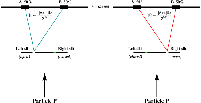
Figure 1: Hypothetical experiment with only two possible outcomes ($A$ and $B$). Left: only the left slit is open. Right: only the right slit is open. Note, each slit is not a simple hole but acts as a filter which projects the particle either to a trajectory with endpoint $A$ or to a trajectory with endpoint $B$.

First, we consider the case in which only the left slit is open (Fig. 1, left side). In order to achieve our goal, the slit is actually not a simple hole in the barrier (out of which a spherical wave would emerge) but a more complicated filter which projects the particle either to a straight trajectory ending in $A$ or to a straight trajectory ending in $B,$ see Fig. 1. In the language of QM, this situation amounts to a wave function $\left|L\right\rangle$ associated to the particle which has gone through the left slit, which is assumed to be:

$$\left|L\right\rangle=\frac{1}{\sqrt{2}}\left(\left|A\right\rangle-\left|B\right\rangle\right)\text{ .}$$ (1)

Then, by simply using the Born rule (i.e., by squaring the coefficient multiplying $\left|A\right\rangle$ or $\left|B\right\rangle$), we predict that the particle ends up either in the endpoint $A$ with probability $50\%$ or in the endpoint $B$ with probability $50\%$. This is indeed what we measure by repeating the experiment many times. As we see, the probability is -for us observer on the screen $S$- a fundamental ingredient of QM, which however enters only in the very last step, i.e. when the measurement comes into the game. The state $\left|L\right\rangle$ is an equal (antisymmetric) superposition of $\left|A\right\rangle$ and $\left|B\right\rangle$, but in a single experiment we do not find a pale spot on $A$ and a pale spot on $B$: we always find the particle either fully in $A$ or in $B.$ It is only after many repetitions of the experiment that we realize that the outcome $A$ and the outcome $B$ are equally probable.

If only the right slit is open (Fig. 1, right side), we have a similar situation in which only two trajectories ending in $A$ and in $B$ are present. The wave function of the particle after having gone through the right slit is denoted by $\left|R\right\rangle$ and is described by the orthogonal combination to $\left|L\right\rangle$:  

$$\text{ }\left|R\right\rangle=\frac{1}{\sqrt{2}}\left(\left|A\right\rangle+\left|B\right\rangle\right)\text{ .}$$ (2)

Then, also in this case one finds the particle in $50\%$ of cases in $A$ and $50\%$ in $B.$

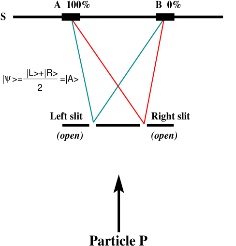
Figure 2: Same setup of Fig. 1, but now both slits are open: interference takes place and all particles hit the screen in $A$.

We now turn to the case in which both slits are open, see Fig. 2. The wave function of the particle is assumed to be the sum of the contributions of the two slits:

$$\left|\Psi\right\rangle=\frac{1}{\sqrt{2}}\left(\left|L\right\rangle+\left|R\right\rangle\right)\text{ ,}$$ (3)

i.e. the contributions of both slits add coherently. A simple calculation shows that

$$\left|\Psi\right\rangle=\left|A\right\rangle\text{ ,}$$ (4)

which means that the particle $P$ always hits the screen in $A$ and never in $B.$ Namely, in $A$ we have a constructive interference, while in $B$ we have a destructive interference. (Notice that the points $A$ and $B$ are not equidistant from the two slits. However, we take the two slits as being close to each other and the points $A$ and $B$ as being far from each other: the difference between the segments $LA$ and $RA$ (and so between $LB$ and $RB$) is assumed to be negligible such that the two contributions of the wave packet of the particle $P$ from the left and right slit arrive almost simultaneously and the depicted interference effect takes place).

In conclusion, we have chosen the language of a two-slit experiment because it is the most intuitive. The price to pay is a slit acting as a filter and not as a simple hole. However, one can easily build analogous setups as the one here described by using photon polarizations, electron spins or equivalent quantum objects, or by using a Mach-Zehnder interferometer, see details in Sec. 2.3.3.

2.2 Detector measuring the path

As a next step we put a detector $D$ right after the two slits (both open). $D$ measures through which hole the particle has passed, without destroying it (see Fig. 3). We analyze the situation in two ways: first, by assuming the collapse of the wave function as induced by $D$ and, second, by studying the entanglement of the particle with the detector. Note, we still assume that we sit on (or watch) the screen $S$ only, but we are not directly connected to the detector $D.$

Collapse: In this case we assume that the detector $D$ generates a collapse of the wave function. Suddenly after the interaction with $D,$ the state of the particle $P$ collapses into $\left|L\right\rangle$ with a probability of $50\%$ or into $\left|R\right\rangle$ with a probability of $50\%$. Then, the state is described by either $\left|L\right\rangle$ or $\left|R\right\rangle$, but not any longer by the superposition of them. As a consequence, we have in half of the cases a situation analogous to having only the left slit open and in the other half to having only the right slit open.

What we will then see on the screen $S$? The probability to find the particle in $A$ is given by

$$P[A]=P[L,A]+P[R,A]=\frac{1}{2}\cdot\frac{1}{2}+\frac{1}{2}\cdot\frac{1}{2}=\frac{1}{2}$$ (5)

where $P[L,A]=1/4$ is the probability that the detector $D$ has measured the particle going through the left slit and then the particle has hit the screen in $A.$ Similarly, $P[R,A]=1/4$ is the probability that the detector $D$ has measured the particle going through the right slit before the latter hits $A.$ A similar description holds for $P[B]=1/2$ with

$$P[B]=P[L,B]+P[R,B]=\frac{1}{2}\cdot\frac{1}{2}+\frac{1}{2}\cdot\frac{1}{2}=\frac{1}{2}\text{ .}$$ (6)

The collapse is obviously part of the standard interpretation of QM, in which a detector is treated as a classical object which induces the collapse of the quantum state. As a result, there is no interference on the screen $S$. As renowned, the standard interpretation does not put any border between what is a classical system and what is a quantum system. Nevertheless, one can interpret the collapse postulate as an effective description of a physical process. Namely, in theories with the collapse of the wave function, the collapse is a real physical phenomenon which takes place when one has a macroscopic displacement of the position wave function of the detector (or, more generally, of the environment). In this framework, somewhere in between the quantum world and the classical macroscopic world, a new physical process takes place which realizes the collapse: this could be, for instance, the stochastic hit in the Ghirardi-Rimini-Weber model [5, 7, 8] or the instability due to gravitation in the Penrose-Diosi approach [6, 10, 11]. Neglecting details, the main point is that such collapse theories realize physically the collapse which is postulated in the standard interpretation and liberates it from inconsistencies. Still, it is an open and well posed physical question if (at least one of) such collapse theories are (is) correct.

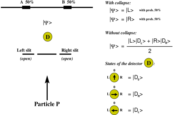
Figure 3: A detector which measures which slit the particle has gone through is placed just after the slits. The wave functions for the collapse and no-collapse scenarios are depicted.

No-collapse: In this case we do not assume that the detector $D$ generates a collapse of the wave function, but we enlarge the whole wave function of the system by including also the wave function of the detector. We assume that, prior to measurement, the detector is in the state $\left|D_{0}\right\rangle$ (we can, for definiteness, think of a old-fashion indicator which points to $0$, see Fig. 3). Then, when both slits are open, the state of the whole system just after having passed through them but not yet in contact with the detector $D$, is given by

$$\left|\Psi\right\rangle=\frac{1}{\sqrt{2}}\left(\left|L\right\rangle+\left|R\right\rangle\right)\left|D_{0}\right\rangle\text{ .}$$ (7)

Then, the particle-detector interaction induces a (we assume very fast) time evolution which generates the following state:

$$\left|\Psi\right\rangle=\frac{1}{\sqrt{2}}\left(\left|L\right\rangle\left|D_{L}\right\rangle+\left|R\right\rangle\left|D_{R}\right\rangle\right)\text{ ,}$$ (8)

where $\left|D_{L}\right\rangle$ ($\left|D_{R}\right\rangle$) describes the pointer of the detector pointing to the left (right). Thus, no collapse is here taken into account, because the whole wave function still includes a superposition of $\left|L\right\rangle$ and $\left|R\right\rangle$, which, however, are now entangled with the detector states $\left|D_{L}\right\rangle$ and $\left|D_{R}\right\rangle$, respectively.

An important point is that the overlap of $\left|D_{L}\right\rangle$ and $\left|D_{R}\right\rangle$ is small:

$$\left\langle D_{L}|D_{R}\right\rangle\simeq 0\text{ ,}$$ (9)

to a very good degree of accuracy. To show it, let us ignore the rest of the detector and the environment and concentrate on the pointer only, which is assumed to be made of $N$ atoms, where $N$ is of the order of the Avogadro constant. The atom $\alpha$ of the pointer is in a superposition of the type $\left(\psi_{L}^{\alpha}(\vec{x})+\psi_{R}^{\alpha}(\vec{x})\right)/\sqrt{2}$, where $\psi_{L}^{\alpha}(\vec{x})$ ($\psi_{R}^{\alpha}(\vec{x})$) is the wave function of the atom when the pointer points to the left (right). We have:

$$\left\langle D_{L}|D_{R}\right\rangle={\displaystyle\prod\limits_{\alpha=1}^{N}}\int d^{3}x\left(\psi_{L}^{\alpha}(\vec{x})\right)^{\ast}\psi_{R}^{\alpha}(\vec{x})\text{ .}$$ (10)

The quantity $\int d^{3}x\left(\psi_{L}^{\alpha}(\vec{x})\right)^{\ast}\psi_{R}^{\alpha}(\vec{x})=\lambda_{\alpha}$ is such that $\left|\lambda_{\alpha}\right|<1$. For a large displacement, $\lambda_{\alpha}$ is itself a very small number (small overlap), but the crucial point is to observe that $\left\langle D_{L}|D_{R}\right\rangle$ is the product of many numbers with modulus smaller then 1. Assuming that $\lambda_{\alpha}=\lambda$ for each $\alpha$ (each atom gets a similar displacement: this assumption is crude but surely sufficient for an estimate), we get

$$\left\langle D_{L}|D_{R}\right\rangle\simeq\lambda^{N}\text{ ,}$$ (11)

which is extremely small for large $N.$ Even if we take $\lambda=0.99$ (which is indeed quite large and actually overestimates the overlap of the wave functions of an atom belonging to macroscopic distinguishable configuration), we obtain

$$\left\langle D_{L}|D_{R}\right\rangle\simeq 0.99^{N_{A}}\sim 10^{-10^{21}}$$ (12)

which is tremendously small.

After having clarified the de facto orthogonality of $\left|D_{L}\right\rangle$ and $\left|D_{R}\right\rangle$, we rewrite the full wave function of the system $\left|S\right\rangle$ as

$$\left|\Psi\right\rangle=\frac{1}{2}\left[\left|A\right\rangle(\left|D_{R}\right\rangle+\left|D_{L}\right\rangle)+\left|B\right\rangle(\left|D_{R}\right\rangle-\left|D_{L}\right\rangle)\right]\text{ .}$$ (13)

Then, the probability to find the particle $P$ in $A$ is obtained (now by using the Born rule, because we are observing the screen $S$):

$$P[A]=P[L,A]+P[R,A]=\frac{1}{2}\cdot\frac{1}{2}+\frac{1}{2}\cdot\frac{1}{2}=\frac{1}{2}$$ (14)

where $P[L,A]=1/4$ is the probability that the system is described by $\left|A\right\rangle\left|D_{L}\right\rangle$ and $P[R,A]=1/4$ the probability that it is described by $\left|A\right\rangle\left|D_{R}\right\rangle.$ A similar situation holds for $P[B]=1/2.$ Thus, also in this case the presence of $D$ causes the disappearance of interference.

The same result is obtained if we use the formalism of the statistical operator, which is defined by $\hat{\rho}=\left|\Psi\right\rangle\left\langle\Psi\right|$ (see, for instance, Refs. [1, 5]). Upon tracing over the detector states (environment states) the reduced statistical operator reads (we use here $\left\langle D_{L}|D_{R}\right\rangle=0$):

$$\hat{\rho}_{red} =\left\langle D_{L}\left|\hat{\rho}\right|D_{L}\right\rangle+\left\langle D_{R}\left|\hat{\rho}\right|D_{R}\right\rangle$$

$$=\left(\begin{array}[c]{cc}\left|A\right\rangle&\left|B\right\rangle\end{array}\right)\left(\begin{array}[c]{cc}\frac{1}{2}&0\\ 0&\frac{1}{2}\end{array}\right)\left(\begin{array}[c]{c}\left\langle A\right|\\ \left\langle B\right|\end{array}\right)\text{ ,}$$ (20)

where the diagonal elements represent $p[A]=p[B]=1/2$ respectively, while the off-diagonal elements vanish in virtue of the (for all practical purposes) orthogonality of $\left|D_{L}\right\rangle$ and $\left|D_{R}\right\rangle$.

Sum up: We find that, for us sitting on the screen $S$, the very same outcome, i.e. the absence of interference, is obtained by applying the collapse postulate as an intermediate step due to the detector $D$ or by considering the whole quantum state -including the detector $D$- and by applying the Born rule only in the very end. This equivalence holds as long as the (anyhow very small) overlap of the detector states of Eq. (12) is neglected (see also the related discussion in Sec. 3). The question is then: do we need the collapse? The second calculation (no-collapse) seems to answer us: ‘no, we don’t’. In this respect, one has a superposition of macroscopic distinct states, which coexist and are nothing else but the branches of the Everett’s or many worlds interpretation (MWI) of QM [16]. Thus, assuming that no collapse takes place brings us quite naturally to the MWI [3, 17, 18, 19, 20].

However, care is needed: in fact, the ‘no collapse’ assumption is a general statement and means also that there is no collapse when the particle $P$ hits the screen $S$ (where our own wave function is part of the game). Let us clarify better this point by going back to the very first case we have studied, in which only the left slit was open and no detector $D$ was present (Fig. 1, left part). The wave function of the particle just before hitting the screen is given by $\left|L\right\rangle=\left(\left|A\right\rangle-\left|B\right\rangle\right)/\sqrt{2}$. But then, after the hit and assuming no collapse, the whole wave function -including us, who are the observers - reads:

$$\left|\Psi\right\rangle =\frac{1}{\sqrt{2}}\left|A\right\rangle\left|\text{Screen recording }A\text{ and we observing }A\right\rangle$$

$$-\frac{1}{\sqrt{2}}\left|B\right\rangle\left|\text{Screen recording }B\text{ and we observing }B\right\rangle\text{ .}$$ (21)

The question is why the coefficient in front of the vector

$$\left|A\right\rangle\left|\text{Screen recording }A\text{ and we observing }A\right\rangle$$

tells us which is the subjective probability of observing $A$ for the observer (us) sitting on the screen. In other words, how does the MWI explain the probabilities according to the Born rule? The Born rule seems to be an additional postulate, which has to be put ad hoc into it. This situation is however not satisfactory, because the main idea of the MWI is to eliminate the collapse from the description of the QM and consequently to derive the standard Born probabilities. Although there are attempts to show that there is no need of postulating the Born rule in this context [21] (see also Ref. [22]), no agreement has been reached up to now [5, 23, 24, 25]. This is indeed an argumentation in favour of the possibility that a collapse really takes place. Surely, ‘real collapse’ scenarios deserve to be studied theoretically and experimentally [5, 6, 7].

Note, up to now we did not mention the decoherence, see e.g. Refs. [2, 26, 27, 28, 29] and refs. therein. This is possible because we have put a detector that makes a measurement by evolving from the state $\left|D_{0}\right\rangle$ into two (almost) orthogonal states $\left|D_{L}\right\rangle$ and $\left|D_{R}\right\rangle$, but actually one can interpret this fast change of the detector state as the result of a decoherence phenomenon. This is however a rather peculiar decoherence, because we have prepared the detector in a particular (low entropic) $\left|D_{0}\right\rangle$ state, which is ‘ready to’ evolve into $\left|D_{L}\right\rangle$ and $\left|D_{R}\right\rangle$ as soon as it interacts with the particle $P$. In Sec. 3 we will describe what changes when the environment, instead of the detector, is taken into account.

2.3 Variants of the setup

2.3.1 The bomb

A simple change of the setup allows us to present the famous Elitzur-Vaidman bomb, first described in Ref. [13] and then experimentally verified in Ref. [30]. We substitute the detector with a ‘bomb’, which can be activated by the particle $P$. We place the bomb only in front of the left slit, see Fig. 4. This means that, if only the left slit is open, the bomb explodes soon after the particle has gone through the slit. If, instead, only the right slit is open, it doesn’t explode. For definiteness and simplicity we assume that the particle is not destroyed nor absorbed by the bomb.

Just as previously, we can interpret the experiment applying either the collapse or by studying the whole wave function. In the collapse approach, the bomb simply makes a measurement. When both slits are open the wave function, before the interaction with the bomb, is given by $\left|\Psi\right\rangle=\left(\left|L\right\rangle+\left|R\right\rangle\right)/\sqrt{2}$: we will have an explosion in $50\%$ of cases and no explosion in the remaining $50\%.$ Notice that in the second case the bomb is doing a null measurement. The very fact that the bomb does not explode means that the particle went to the right slit (we assume 100% efficiency in our ideal experiment). When the bomb explodes there is a collapse into $\left|\Psi\right\rangle=\left|L\right\rangle$, when it doesn’t into $\left|\Psi\right\rangle=\left|R\right\rangle.$ Then, we have a situation which is very similar to the case of the detector $D$ which we have studied previously: no interference on the screen $S$ is observed, but we observe the particle in the endpoint $A$ and $B$ with probability $1/2$ each.

If we do not assume the collapse of the wave function, the whole wave function is given by (after interaction with the bomb)

$$\left|\Psi\right\rangle =\frac{1}{\sqrt{2}}\left(\left|L\right\rangle\left|B_{E}\right\rangle+\left|R\right\rangle\left|B_{0}\right\rangle\right)$$

$$=\frac{1}{2}\left[\left|A\right\rangle(\left|B_{0}\right\rangle+\left|B_{E}\right\rangle)+\left|B\right\rangle(\left|B_{0}\right\rangle-\left|B_{E}\right\rangle)\right]$$ (22)

where $\left|B_{0}\right\rangle$ is the state describing the unexploded bomb and $\left|B_{E}\right\rangle$ the exploded one. Obviously, as in Eq. (12), we have $\left\langle B_{E}|B_{0}\right\rangle\simeq 0.$ Again and just as before no interference is seen on $S$ but the two outcomes $A$ and $B$ are equiprobable. Clearly, no difference between assuming the collapse or not is found, but the interesting fact is that the non-explosion of the bomb is enough to destroy interference.

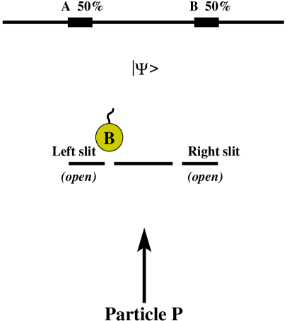
Figure 4: Variant of the Elitzur-Vaidman experiment: a bomb is placed just after the left slit.

If, instead of the bomb we put a fake bomb (referred to as the dud bomb, which has the very same aspect of the real functioning bomb but does not interact at all with the particle $P$), the wave function of the system is given by

$$\left|\Psi\right\rangle=\frac{1}{\sqrt{2}}\left(\left|L\right\rangle+\left|R\right\rangle\right)\left|B_{0}^{dud}\right\rangle=\left|A\right\rangle\left|B_{0}^{dud}\right\rangle$$ (23)

where $\left|B_{0}^{dud}\right\rangle$ describes the wave function of the dud bomb. In this case, there is interference and the particle $P$ always ends up in $A$.

Then, the amusing part comes: if we do not know if the bomb is a dud or not, we can –in some but not all cases– find out by placing it in front of the left slit. If there is no explosion and the particle ends up in $B,$ we deduce for sure that the bomb is real. Namely, this outcome is not possible for a dud, see Eq. (23). Note, we have deduced that the bomb is ‘good’ without making it explode (that would be easy: just send the particle $P$ toward the bomb, if it goes ‘boom’ it was real). This situation occurs in $25\%$ of cases in which a functioning bomb is placed behind the slit, see Eq. (22): we can immediately ‘save’ $25\%$ of the good bombs. Conversely, in $50\%$ of cases the good bomb simply explodes and we lose it (then, the particle $P$ goes to either $A$ (25%) or to $B$ (25%)). In the remaining $25\%$ the good bomb does not explode, but the particle $P$ hits $A.$ Then, we simply do not know if the bomb is good or fake: this situation is compatible with both hypotheses. We can, however, repeat the experiment: in the end, we will be able to save $1/4$ $+1/4\cdot 1/4+...=1/3$ of the functioning bombs.

2.3.2 The idler particle and the delayed choice experiment

Another interesting configuration is obtained by assuming that a second entangled particle, denoted as $I$ (for idler), is emitted when $P$ goes through the slit(s). The system is built in the following way: if the particle $P$ goes through the left slit, the particle $I$ is described by the state $\left|I_{L}\right\rangle$. Similarly, when the particle $P$ goes to the right slit, the particle $I$ is described by the state $\left|I_{R}\right\rangle$. We assume that the two idler states are orthogonal: $\left\langle I_{L}|I_{R}\right\rangle=0.$ This situation resembles closely that of delayed choice experiments [14, 15].

When both slits are open the whole wave function of the system is given by:

$$\left|\Psi\right\rangle =\frac{1}{\sqrt{2}}\left(\left|L\right\rangle\left|I_{L}\right\rangle+\left|R\right\rangle\left|I_{R}\right\rangle\right)$$

$$=\text{ }\frac{1}{2}\left[\left|A\right\rangle(\left|I_{R}\right\rangle+\left|I_{L}\right\rangle)+\left|B\right\rangle(\left|I_{R}\right\rangle-\left|I_{L}\right\rangle)\right]\text{ .}$$ (24)

The particle $I$ is entangled with $P$, but being the latter a microscopic object, we surely cannot apply the collapse hypothesis because the particle $I$ is not a measuring apparatus.

Do we have interference on the screen $S$ in this case? The answer is clear: no. The states $\left|A\right\rangle\left|I_{L}\right\rangle,$ $\left|A\right\rangle\left|I_{R}\right\rangle,$ $\left|B\right\rangle\left|I_{L}\right\rangle,$ $\left|B\right\rangle\left|I_{R}\right\rangle$ represent a basis of this system, thus the probability to obtain $\left|A\right\rangle$ (that is, the probability of $P$ hitting $S$ in $A$) is $1/4+1/4=1/2.$ So for $B.$ The presence of the entangled idler state destroys the interference on $S.$

It is sometime stated that this result is a consequence of the fact that the state of the idler particle $I$ carries the information of which way $P$ has followed. For this reason, the interference has disappeared (this is a modern reformulation of the complementarity principle). However, such expressions, although appealing, are often too vague and need to be taken with care.

As a next step we study what happens if we perform a measurement on the particle $I$. We study separately two distinct types of measurements.

Measuring $I$ in the $\left|I_{L}\right\rangle$-$\left|I_{R}\right\rangle$ basis.

First, we perform a measurement which tells us if the state of the idler particle is $\left|I_{L}\right\rangle$ or $\left|I_{R}\right\rangle.$ For simplicity, we apply the collapse hypothesis (as usual, the results would not change by keeping track of the whole unitary quantum evolution). But first, we have to clarify the following issue: when do we perform the measurement on $I$? We have two possibilities:

• If we measure the state of $I$ before the particle $S$ hits the screen, the wave function reduces to $\left|L\right\rangle\left|I_{L}\right\rangle$ or to $\left|R\right\rangle\left|I_{R}\right\rangle$ with $50\%$ probability, respectively. Then, the screen $S$ performs a second measurement: we find -as usual- 50% of times $A$ ($25\%$ $\left|A\right\rangle\left|I_{L}\right\rangle$ and $25\%$ $\left|A\right\rangle\left|I_{R}\right\rangle$) and 50% of times $B$ ($25\%$ $\left|B\right\rangle\left|I_{L}\right\rangle$ and $25\%$ $\left|B\right\rangle\left|I_{R}\right\rangle$).

• If, instead, the particle $P$ arrives first on the screen $S$, the quantum state collapses into $\left|A\right\rangle(\left|I_{R}\right\rangle+\left|I_{L}\right\rangle)/\sqrt{2}$ in $50\%$ of cases ($A$ has clicked), or into $\left|B\right\rangle(\left|I_{R}\right\rangle-\left|I_{L}\right\rangle)/\sqrt{2}$ in the other $50\%$ of cases ($B$ has clicked). The subsequent measurement of the $I$ particle will then give $\left|I_{L}\right\rangle$ or $\left|I_{R}\right\rangle$ ($50\%$ each).

In conclusion, we realize that it is absolutely not relevant which experiment is done before the other. In particular, for us sitting on the screen $S$, it does not matter at all when and if the measurement of the idler state is performed. We simply see no interference.

Measuring $I$ in the $(\left|I_{R}\right\rangle+\left|I_{L}\right\rangle)/\sqrt{2}$-$(\left|I_{R}\right\rangle-\left|I_{L}\right\rangle)/\sqrt{2}$ basis.

Being the particle $P$ entangled with another particle and not with a macroscopic state, we can also decide to perform a different kind of measurement on $I.$ For instance, we can put a detector measuring $I$ by projecting onto the basis $(\left|I_{R}\right\rangle+\left|I_{L}\right\rangle)/\sqrt{2}$ and $(\left|I_{R}\right\rangle-\left|I_{L}\right\rangle/\sqrt{2}$. If we do this measurement before the particle $P$ has hit the screen $S,$ we have the following outcome as a consequence of the collapse induced by the $I$-detector:

$$\left|\Psi\right\rangle =\left|A\right\rangle(\left|I_{R}\right\rangle+\left|I_{L}\right\rangle)/\sqrt{2}\text{ with prob. 50\% ;}$$ (25)

$$\left|\Psi\right\rangle =\left|B\right\rangle(\left|I_{R}\right\rangle-\left|I_{L}\right\rangle)/\sqrt{2}\text{ with prob. 50\% .}$$ (26)

In the former case, the particle $P$ will surely hit $S$ in $A,$ in the latter in $B.$

One sometimes interpret the experiment in the following way: the detector measuring the state of $I$ as being either $(\left|I_{R}\right\rangle+\left|I_{L}\right\rangle)/\sqrt{2}$ or $(\left|I_{R}\right\rangle-\left|I_{L}\right\rangle/\sqrt{2}$ ‘erases the which-way information’. When the detector measures $(\left|I_{R}\right\rangle+\left|I_{L}\right\rangle)/\sqrt{2}$ we still have interference and we see the particle $P$ in the position $A$, just as the case with two open slits (Fig. 2). In the other case, when the detector measures $(\left|I_{R}\right\rangle-\left|I_{L}\right\rangle)/\sqrt{2}$, we also have a kind of interference in which the final position $B$ is the only outcome. In the language of Ref. [14], one speaks of ‘fringes’ in the former case, and of ‘anti-fringes’ in the latter.

However, care is needed: for us sitting on $S$, if we do not know which measurement is performed on $I,$ we simply see that no interference occurs ($50\%$-$A$ and $50\%$-$B$). But, if we could then speak with a colleague working with the $I$-detector, we would realize that, each time we have measured $A$ he has found the state $(\left|I_{R}\right\rangle+\left|I_{L}\right\rangle)/\sqrt{2},$ while each time we have measured $B$ he has found $(\left|I_{R}\right\rangle-\left|I_{L}\right\rangle/\sqrt{2}.$ Thus, we have a correlation of our results (measurement of the screen $S)$ with those of the $I$-detector. This is actually no surprise if we look at the quantum state of Eq. (24). This statement is indeed more precise than the statement of having interference because we have erased the which-way information. Namely, we do not have interference.

Indeed, we can perform the measurement of $I$ even after (in principle much time after) the screen $S$ has measured $P$ in either $A$ or $B.$ Here the name ‘delayed choice’ comes from: we choose if we retain the which-way information or not. Still, the result is the same because there is no influence on the time-ordering of the measurements. If the measurement of the screen $S$ occurs first, we have a collapse onto the very same Eqs. (25)-(26). Then, a measurement of the idler particle $I$ would simply find either $(\left|I_{R}\right\rangle+\left|I_{L}\right\rangle)/\sqrt{2}$ (correlated with $A$) and $(\left|I_{R}\right\rangle-\left|I_{L}\right\rangle)/\sqrt{2}$ (correlated with $B$). For sure, there is no change of the past by a measurement of the idler state, but simply a correlation of states. Still, such a very interesting setup visualizes many of the peculiarities of QM and can be used for quantum cryptography.

2.3.3 Realizations of the setup

In a two-slit experiment all the peculiarities of QM are evident due to the fact that the particle $P$ follows (at least) two paths at the same time. This is extremely fascinating as well as counterintuitive for our imagination based on a childhood with rolling ‘classical’ marbles. However, as already mentioned in Sec. 1.1, a simple implementation of the two-slit experiment does not produce only two possible outcomes, but gives rise to a superposition of waves with many maxima and minima. In the following we present two possible realizations of our Gedankenexperiment which do not make use of slits.

An interference experiment in which only two outcomes are possible can be realized by using particles with spin $1/2$ (such as electrons in a Stern-Gerlach-type experiment) or photons (spin 1, but due to gauge invariance only two polarizations are realized). Clearly, all the QM features do not depend on which particle or on which quantum number are implemented, but solely on the presence of superpositions and on the effect of measurements. In the case of photon polarizations we can use the fact that a photon can be horizontally or vertically polarized (corresponding to the kets $\left|h\right\rangle$ and $\left|v\right\rangle$ respectively). In our analogy, the state $\left|h\right\rangle$ corresponds to the state of our particle $P$ coming out from the left slit, $\left|h\right\rangle\equiv\left|L\right\rangle,$ and similarly $\left|v\right\rangle$ from the right slit, $\left|v\right\rangle\equiv\left|R\right\rangle.$ Then, we place a detector which acts as the screen $S$ by making a measurement in the basis $\left|A\right\rangle=(\left|v\right\rangle+\left|h\right\rangle)/\sqrt{2}$ and $\left|B\right\rangle=(\left|v\right\rangle-\left|h\right\rangle)/\sqrt{2}$. In addition, we can place a second detector which plays the role of the detector $D$ by measuring the polarization in the $\left|h\right\rangle$-$\left|v\right\rangle$ basis. Indeed, in this case we do not need to send the photons along two different paths, because the polarization d.o.f. is enough for our purposes.

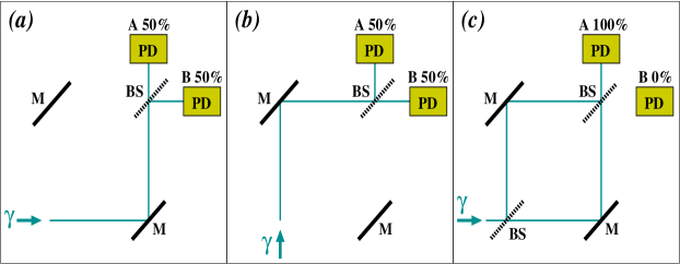
Figure 5: The Mach-Zehnder interferometer. M stands for mirror, BS for beam splitter, and PD for photon detector. The case (a) is analogous to having only the left slit open (Fig. 1, left side), (b) to only the right slit open (Fig. 1, right side), (c) to both slits open (Fig. 2).

Another possible realization of our setup is the Mach-Zehnder interferometer [31], see Fig. 5, which makes use of beam splitters. When a photon is sent to the path of Fig. 5.a (denoted as path-1), both photon counters $A$ and $B$ can detect the photon with a probability of 50% . For our analogy, we have $\left|path\text{-1}\right\rangle\equiv\left|L\right\rangle$. Similarly, when the photon is sent to the path of Fig. 5.b (path-2), we hear a click in $A$ or in $B$ with 50% probability. For the analogy: $\left|path\text{-2}\right\rangle\equiv\left|R\right\rangle$. When a beam splitter is put in the beginning of the setup, after the photon passes through, we get a superposition $(\left|path\text{-1}\right\rangle+\left|path\text{-2}\right\rangle)/\sqrt{2}$ (Fig. 5.c). The inclusion of the detector $D$, the bomb, entangled particle(s) as well as the environment can be easily carried out.

In the end, notice that Mach-Zehnder interferometers can be constructed by using neutrons instead of photons. The so-called neutron interferometers (see the recent review paper [32] and refs. therein) can be very well controlled and allow to experimentally study quantum systems to a great level of accuracy.

3 Collapse vs no-collapse: there is a difference

In this section we show that there is a difference between the collapse and no-collapse scenarios. To this end, instead of having a detector, a bomb, or an idler entangled state, we assume that the space between the slits and the screen is not the vacuum. Then, we study the time evolution of the environment which interacts with the particle $P$. This interaction is assumed to be soft enough not to absorb or kick away the particle in such a way that the final outcomes on the screen $S$ are still the endpoints $A$ or $B$.

Before the particle $P$ goes through the slit(s), the environment is described by the state $\left|E_{0}\right\rangle$. First, we study the case in which only the left slit is open. Denoting as $t=0$ the time at which $P$ passes through the left slit, the wave function of the environment evolves as function of time $t$ as

$$\left|\Psi(t)\right\rangle=\left|L\right\rangle\left|E_{L}(t)\right\rangle\text{ ,}$$ (27)

where by construction $\left|E_{L}(0)\right\rangle=\left|E_{0}\right\rangle$. Similarly, if only the right slit is open, at the time $t$ the system is described by $\left|\Psi(t)\right\rangle=\left|R\right\rangle\left|E_{R}(t)\right\rangle$ with $\left|E_{R}(0)\right\rangle=\left|E_{0}\right\rangle$.

We now turn to the case in which both slits are open. It is important to stress that, by assuming a weak interaction of the particle $P$ with the environment, we surely do not have -at first- a collapse of the wave function, but an evolution of the whole quantum state given by:

$$\left|\Psi(t)\right\rangle =\frac{1}{\sqrt{2}}\left(\left|L\right\rangle\left|E_{L}(t)\right\rangle+\left|R\right\rangle\left|E_{R}(t)\right\rangle\right)$$

$$=\frac{1}{2}\left[\left|A\right\rangle(\left|E_{R}(t)\right\rangle+\left|E_{L}(t)\right\rangle)+\left|B\right\rangle(\left|E_{R}(t)\right\rangle-\left|E_{L}(t)\right\rangle)\right]\text{ .}$$ (28)

This is indeed very similar to the detector case, but there is a crucial aspect that we now take into consideration. The state $\left|E_{L}(t)\right\rangle$ and $\left|E_{R}(t)\right\rangle$ coincide at $t=0$ and then smoothly depart from each other. At the time $t$ we assume to have

$$c(t)=\left\langle E_{L}(t)|E_{R}(t)\right\rangle=e^{-\lambda t}\text{ .}$$ (29)

(where $c(t)$ is taken to be real for simplicity). This is nothing else than a gradual decoherence process. The states of the environment entangled with $\left|L\right\rangle$ and $\left|R\right\rangle$ overlap less and less by the time passing. The constant $\lambda$ describes the speed of the decoherence and depends on the number of particles involved and the intensity of the interaction. Note, strictly speaking, this non-orthogonality is also present in the case of the detector (if no collapse is assumed), but the overlap is amazingly small, see the estimate in Eq. (12). (In the case of the detector $D$ of Sec. 2.2, $\lambda$ is very large and consequently $\lambda^{-1}$ is a very short time scale, shorter than any other time scale in the setup of Fig. 3. For that reason we assumed that the detector state evolved for all practical purposes instantaneously from the ready-state (pointer up) to pointing either to the left or to the right.)

Now we ask the following question: what is the probability that the particle $P$ hits the screen in $A$? We assume that the particle $P$ hits the screen at the time $\tau.$ At this instant, the state is given by $\left|\Psi(\tau)\right\rangle$ with $\left\langle E_{L}(\tau)|E_{R}(\tau)\right\rangle=c(\tau)$.

We now present the mathematical steps leading to $p[A,\tau]$, which, although still simple, are a bit more difficult than the previous ones. The reader who is only interested in the result can go directly to Eq. (34).

At the time $\tau$ we express the state $\left|E_{L}(\tau)\right\rangle$ as

$$\left|E_{L}(\tau)\right\rangle=c(\tau)\left|E_{R}(\tau)\right\rangle+\sum_{\alpha}b_{\alpha}(\tau)\left|E_{R,\perp}^{\alpha}(\tau)\right\rangle$$ (30)

where the summation over $\alpha$ includes all states of the environment which are orthogonal to $\left|E_{R}(\tau)\right\rangle$: $\left\langle E_{R,\perp}^{\alpha}(\tau)|E_{R}(\tau)\right\rangle=0$. This expression is possible because the set $\{E_{R}(\tau),E_{R,\perp}^{\alpha}(\tau)\}$ represents a orthonormal basis for the environment state. Its explicit expression is be extremely complicated, but we do not need to specify it. The normalization of the state $\left|E_{L}(\tau)\right\rangle$ implies that

$$\left|c(\tau)\right|^{2}+\sum_{\alpha}\left|b_{\alpha}(\tau)\right|^{2}=1.$$ (31)

Then, the state of the system at the instant $\tau$ is given by the superposition

$$\left|\Psi(\tau)\right\rangle =\frac{1}{2}\left[1+c(\tau)\right]\left|A\right\rangle\left|E_{R}(\tau)\right\rangle+\frac{1}{2}\left|A\right\rangle\sum_{\alpha}b_{\alpha}(\tau)\left|E_{R,\perp}^{\alpha}(\tau)\right\rangle$$

$$+\frac{1}{2}\left[1-c(\tau)\right]\left|B\right\rangle\left|E_{R}(\tau)\right\rangle+\frac{1}{2}\left|B\right\rangle\sum_{\alpha}b_{\alpha}(\tau)\left|E_{R,\perp}^{\alpha}(\tau)\right\rangle\text{ .}$$ (32)

At the time $\tau$ the probability of the particle $P$ hitting $A$ is given by

$$p[A,\tau]=\frac{1}{4}\left|1+c(\tau)\right|^{2}+\frac{1}{4}\sum_{\alpha}\left|b_{\alpha}(\tau)\right|^{2}=\frac{1}{4}\left|1+c(\tau)\right|^{2}+\frac{1}{4}\left(1-\left|c(\tau)\right|^{2}\right)\text{ ,}$$ (33)

where in the last step we have used Eq. (31). A simple calculation leads to

$$p[A,\tau]=\frac{1}{2}+\frac{1}{2}c(\tau)=\frac{1}{2}+\frac{1}{2}e^{-\lambda\tau}\text{ }.$$ (34)

A similar calculation leads to the probability of the particle $P$ hitting $S$ in $B$ as

$$p[B,\tau]=\frac{1}{2}-\frac{1}{2}c(\tau)=\frac{1}{2}-\frac{1}{2}e^{-\lambda\tau}\text{ .}$$ (35)

We see that ‘a bit’ of interference is left (no matter how large the time interval $\tau$ is):

$$p[A,\tau]-p[B,\tau]=e^{-\lambda\tau}\text{ ,}$$ (36)

showing that there is always an (eventually very slightly) enhanced probability to see the particle in $A$ rather than in $B.$

Notice that the very same result is found by using the reduced statistical operator:

$$\hat{\rho}_{red}(\tau) =\left\langle E_{R}(\tau)\left|\hat{\rho}(\tau)\right|E_{R}(\tau)\right\rangle+\sum_{\alpha}\left\langle E_{R,\perp}^{\alpha}(\tau)\left|\hat{\rho}(\tau)\right|E_{R,\perp}^{\alpha}(\tau)\right\rangle$$

$$=\left(\begin{array}[c]{cc}\left|A\right\rangle&\left|B\right\rangle\end{array}\right)\left(\begin{array}[c]{cc}p[A,\tau]&c(\tau)\\ c(\tau)&p[B,\tau]\end{array}\right)\left(\begin{array}[c]{c}\left\langle A\right|\\ \left\langle B\right|\end{array}\right)\text{ }$$ (42)

where $\hat{\rho}(\tau)=\left|\Psi(\tau)\right\rangle\left\langle\Psi(\tau)\right|$. The diagonal elements are the usual Born probabilities, while the non-diagonal elements quantify the overlap of the two branches and become very small for increasing time. (A related subject to the quantum evolution described here is that of the weak measurement, in which the ‘measurement’ is performed by a weak interaction and thus a unitary evolution of the whole system is taken into account, see the recent review [33] and refs. therein.)

All these considerations do not require any collapse of the wave function due to the environment (see also Ref. [34]). Indeed, if we replace the environment with the detector $D$ of Sec. 2 (which was nothing else than a particular environment), the whole discussion is still valid (but see the comments on time scale after Eq. (29)). The only point when the Born rule enters is when we see the particle being either in $A$ or in $B,$ but -as we commented previously- in this no-collapse MWI scenario, we do not know why the Born rule applies [23, 24]. In this sense, decoherence alone is not a solution of the measurement problem [35]. The wave function is still a superposition of different and distinguishable macroscopic states. Still, because of decoherence, these states (branches) become almost orthogonal, thus decoherence is an important element of the MWI although it does not explain the emergence of probabilities.

What do theories with the collapse of the wave function predict? As long as few particles of the environment are involved (i.e., at small times), for sure we do not have any collapse and the entanglement in Eq. (28) is the correct description of the system. Namely, we know that interference effects occur for systems which contains about $1000$ (and even more) particles [36]. But, if we wait long enough we can reach a critical number of particles at which the collapse takes place. Thus, simplifying the discussion as much as possible, according to collapse models there should be a critical time-interval $\tau^{\ast}$ at which the probability $p[A,\tau]$ suddenly jumps to $1/2$ [37]:

$$p[A,\tau]=\left\{\begin{array}[c]{c}\frac{1}{2}+\frac{1}{2}e^{-\lambda\tau}\text{ for }\tau<\tau^{\ast}\text{ ;}\\ \\ \frac{1}{2}\text{ for }\tau\geq\tau^{\ast}\text{ .}\end{array}\right.$$ (43)

Indeed, such a sudden jump is an oversimplification, but is enough for our purposes: it shows that a new phenomenon, the collapse, takes place. In Fig. 6 we show schematically the difference between the ‘no-collapse’ and the ‘collapse’ cases. Obviously, if $\tau^{\ast}$ is very large, it becomes experimentally very difficult to distinguish the two curves, but the qualitative difference between them is clear.

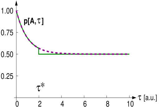
Figure 6: The quantity $p[A,\tau]$ is plotted as function of $\tau.$ The dashed line represents the prediction of the unitary evolution of Eq. (28). The solid line represents the prediction of the collapse hypothesis of Eq. (43): if the detection of the screen takes place for $\tau$ larger than the critical value $\tau^{\ast}$, the state has collapsed to either $A$ or $B,$ therefore $p[A,\tau>\tau^{\ast}]=1/2$. Note, we use arbitrary units. The choice of $\tau^{\ast}$ is also arbitrary and serves to visualize the effect (it is expected to be much larger in reality).

In Ref. [38] the gradual appearance of decoherence due to interaction of electrons with image charges has been experimentally observed. This is analogous to our Eq. (34). (For other decoherence experiment see Ref. [29] and refs. therein.) Indeed, it would be very interesting to study decoherence in a setup with only two outcomes, for instance with the help of a Mach-Zehnder interferometer or by using neutron interferometers. Namely, even if the distinction between collapse/non-collapse is not yet reachable [7], a clear demonstration of decoherence and the experimental verification of Eq. (34) would be useful on its own.

As a last step, we show that the behavior $p[A,t]=1/2$ $\forall t>\tau^{\ast}$ is a peculiarity of the collapse approach which is impossible if only a unitary evolution is taken into account. The proof makes use of the Hamiltonian $H$ of the whole system (particle+slits+environment), for which we assume that $\left\langle R\left|H\right|L\right\rangle=\left\langle L\left|H\right|R\right\rangle=0$, i.e. the full Hamiltonian does not mix the states $\left|L\right\rangle$ and $\left|R\right\rangle$. (This is indeed a quite general assumption for the type of problems that we study: once the particle has gone through the left slit, its wave function is $\left|L\right\rangle$ and stays such (and viceversa for $\left|R\right\rangle).$ Similarly, in the example of a (photon or neutron) Mach-Zehnder interferometer, after the first beam-splitter the path is either the lower or the upper and the whole Hamiltonian does not mix them.) It then follows that:

$$\left|\Psi(t)\right\rangle =e^{-iHt}\frac{1}{\sqrt{2}}\left(\left|L\right\rangle\left|E_{0}\right\rangle+\left|R\right\rangle\left|E_{0}\right\rangle\right)$$

$$=\frac{1}{\sqrt{2}}\left(\left|L\right\rangle e^{-iH_{L}t}\left|E_{0}\right\rangle+\left|R\right\rangle e^{-iH_{R}t}\left|E_{0}\right\rangle\right)$$ (44)

where we have expressed $\left|E_{L}(t)\right\rangle=e^{-iH_{L}t}\left|E_{0}\right\rangle$ and $\left|E_{R}(t)\right\rangle=e^{-iH_{R}t}\left|E_{0}\right\rangle$ by introducing the Hamiltonians $H_{L}=\left\langle L\left|H\right|L\right\rangle$ and $H_{R}=\left\langle R\left|H\right|R\right\rangle$ which act in the subspace of the environment. (These expressions hold because $H^{n}\left|L\right\rangle\left|E_{0}\right\rangle=\left|L\right\rangle H_{L}^{n}\left|E_{0}\right\rangle$ for each $n$). The overlap $c(t)$ defined in Eq. (29) can be formally expressed as

$$c(t)=\left\langle E_{L}(t)|E_{R}(t)\right\rangle=\left\langle E_{0}\left|e^{-i(H_{R}-H_{L})t}\right|E_{0}\right\rangle\text{ .}$$ (45)

Being $H_{L}$ and $H_{R}$ Hermitian, also $H_{R}-H_{L}$ is such. For a finite number of degrees of freedom of the system, the quantity $c(t)$ shows a (almost) periodic behavior and returns (very close) to the initial value $1$ in the so-called Poincaré duration time (which can be very large for large systems). It is then excluded that $c(t)$ vanishes for $t>\tau^{\ast}.$ (At most, it can vanish for certain discrete times, see Sec. 4, but not continuously). Even in the limit of an infinite number of states, the quantity $c(t)$ does not vanish but approaches smoothly zero for $t\rightarrow\infty$.

4 Entanglement with a non-orthogonal idler state

As a last example, we design an ideal setup in which the environment is represented again by a single particle, the idler state (see Sec. 2.3.2). However, we assume now that a time-evolution of the idler state takes place:

$$\left|\Psi(t)\right\rangle=\frac{1}{\sqrt{2}}\left(\left|L\right\rangle\left|E_{L}(t)\right\rangle+\left|R\right\rangle\left|E_{R}(t)\right\rangle\right)\text{ ,}$$ (46)

with the ‘environment’ states now expressed in terms of the orthonormal idler-basis $\{\left|I_{1}\right\rangle,\left|I_{2}\right\rangle\}$.

$$\left|E_{L}(t)\right\rangle =\left|I_{1}\right\rangle\text{ ,}$$ (47)

$$\left|E_{R}(t)\right\rangle =\cos(\omega t)\left|I_{1}\right\rangle+\sin(\omega t)\left|I_{2}\right\rangle\text{ .}$$ (48)

Thus, while $\left|E_{L}(t)\right\rangle=\left|I_{1}\right\rangle$ is a constant over time, we assume that $\left|E_{R}(t)\right\rangle$ rotates in the space spanned by $\left|I_{1}\right\rangle$ and $\left|I_{2}\right\rangle.$ Then, we can rewrite $\left|\Psi(t)\right\rangle$ as

$$\left|\Psi(t)\right\rangle =\frac{1}{2}\left|A\right\rangle\left[\left(1+\cos(\omega t)\right)\left|I_{1}\right\rangle+\sin(\omega t)\left|I_{2}\right\rangle\right]$$

$$+\frac{1}{2}\left|B\right\rangle\left[\left(-1+\cos(\omega t)\right)\left|I_{1}\right\rangle+\sin(\omega t)\left|I_{2}\right\rangle\right]\text{ .}$$ (49)

The probability $p[A,\tau]$ is given by

$$p[A,\tau]=\frac{1}{2}+\frac{1}{2}\cos(\omega\tau)$$ (50)

where $\tau$ is the time at which the particle $P$ hits the screen.

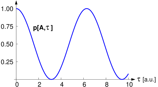
Figure 7: Quantity $p[A,\tau]$ as function of $\tau$ in the case of entanglement with an idler state according to Eq. (49).

In conclusion, in a real implementation of this simple idea, it would be interesting to see the appearance and the disappearance of interference (with both fringes and antifringes) as function of the time of flight $\tau$, see Fig. 7. It should be however stressed that the full interaction Hamiltonian does not act on the idler state alone. Indeed, the corresponding Hamiltonian has the form

$$H=\alpha(\left|R\right\rangle\left|I_{1}\right\rangle\left\langle R\right|\left\langle I_{2}\right|+\text{ h.c.}).$$ (51)

This is indeed a quite peculiar type of interaction because the idler state rotates only if the particle $P$ is in the state $\left|R\right\rangle$ (in the language of Sec. 4, it means: $H_{L}=0,$ $H_{R}=\alpha(\left|I_{1}\right\rangle\left\langle I_{2}\right|+$ h.c.$).$). This implies that the spatial trajectory of both states $\left|I_{1}\right\rangle$ and $\left|I_{2}\right\rangle$ must be the same, otherwise the overlap $\left\langle E_{L}(t)|E_{R}(t)\right\rangle$ would be an extremely small number and the effect that we have described would not take place.

5 Conclusions

We have presented an ideal interference experiment in which we have compared the unitary evolution and the existence of a collapse of the wave function. We have analyzed the case in which a detector measures the which-way information and we have shown that the collapse postulate as well as the no-collapse unitary evolution lead to the same outcome: the disappearance of interference on the screen. In the unitary (no-collapse) evolution, this is true only if the states of the detector are orthogonal. This is surely a very good, but not exact, approximation. It was then possible to describe within the very same Gedankenexperiment two astonishing quantum phenomena: the Elitzur-Vaidman bomb and the delayed-choice experiment.

We have then turned to a description of the entanglement with the environment. The phenomenon of decoherence ensures that the interference smoothly disappears. However, as long as the quantum evolution is unitary, it never disappears completely. Conversely, the real collapse of the wave function introduces a new kind of dynamics which is not part of the linear Schrödinger equation. While the details differ according to which model is chosen [7], the main features are similar: a quantum state in which one has a delocalized object (superposition of ‘here’ and ‘there’) is not a stable configuration, but is metastable and decays to a definite position (either ‘here’ or ‘there’). In conclusion, the collapse and the no-collapse views are intrinsically different, as Fig. 5 shows. At a fundamental level, the unitary (no-collapse) evolution leads quite naturally to the many worlds interpretation in which also detectors and observers are included in a superposition (for a different view see the Bohm interpretation [39]).

Even if the distinction between the collapse and the no-collapse alternatives is probably still too difficult to be detected at the moment, the demonstration of decoherence in an experiment with two final states would be an interesting outcome on its own (see the dashed curve in Fig. 6) . Also a situation in which an entangled particle is emitted in such a way that an ‘oscillating interference’ takes place (see Fig. 7) might be an interesting possibility.

A further promising line of research to test the existence of the collapse of the wave function is the theoretical and experimental study of unstable quantum systems. The non-exponential behavior of the survival probability for short times renders the so-called Zeno and Anti-Zeno effects possible [40, 41, 42, 43]: these are modifications of the survival probability due to the effect of the measurement, which have been experimentally observed [44]. The measurement of an unstable system (for instance, the detection of the decay products) can be modelled as a series of ideal measurements in which the collapse of the wave function occurs, but can also be modelled through a unitary evolution in which the wave function of the detector is taken into account and no collapse takes place [45, 46, 47]. Then, if differences between these types of measurement appear, one can test how a detector is performing a certain measurement [48]. Quite remarkably, such effects are not restricted to nonrelativistic QM, but hold practically unchanged also in the context of relativistic quantum field theory [49] and are therefore applicable in the realm of elementary particles.

In conclusions, Quantum Mechanics still awaits for better understanding in the future. It is surely of primary importance to test the validity of (unitary) standard QM for larger and heavier bodies. In this way the new collapse dynamics, if existent, may be discovered.

Acknowledgment: These reflections arise from a series of seminars on ‘Interpretation and New developments of QM’ and lectures ‘Decays in QM and QFT’, which took place in Frankfurt over the last 4 years. The author thanks Francesca Sauli, Stefano Lottini, Giuseppe Pagliara, and Giorgio Torrieri for useful discussions. Stefano Lottini is also aknwoledged for a careful reading of the manuscript and for help in the preparation of the figures.

References

- [1] J. J. Sakurai, Modern Quantum Mechanics, Addison-Wesley Publishing Company (1994).
- [2] R. Omnes, Interpretation Of Quantum Mechanics, Princenton, Princeton University Press, 1994.
- [3] M. Tegmark and J. A. Wheeler, Wiss. Dossier 2003N1 (2003) 6] [quant-ph/0101077].
- [4] J. S. Bell, (1981) 41; J. S. Bell, (1964) 195; J. S. Bell, (1966) 447.
- [5] A. Bassi and G. C. Ghirardi, Phys. Rept. 379 (2003) 257 [quant-ph/0302164].
- [6] R. Penrose, The road to reality: A complete guide to the laws of the Universe, Vintage Book, London.
- [7] A. Bassi, K. Lochan, S. Satin, T. P. Singh and H. Ulbricht, Rev. Mod. Phys. 85 (2013) 471 [arXiv:1204.4325 [quant-ph]].
- [8] G. C. Ghirardi, O. Nicrosini, A. Rimini and T. Weber, Nuovo Cim. B 102 (1988) 383.
- [9] P. M. Pearle, Phys. Rev. D 13 (1976) 857.
- [10] R. Penrose, (1996) 581.
- [11] L. Diosi, J. Phys. A 21 (1988) 2885.
- [12] T. P. Singh, J. Phys. Conf. Ser. 174 (2009) 012024 [arXiv:0711.3773 [gr-qc]].
- [13] A. C. Elitzur and L. Vaidman, 23, Issue 7 987-997 (1993) [hep-th/9305002].
- [14] Y. -H. Kim, R. Yu, S. P. Kulik, Y. H. Shih and M. .O. Scully, Phys. Rev. Lett. 84 (2000) 1 [quant-ph/9903047].
- [15] S. P. Walborn, M. O. Terra Cunha, S. Padua and C. H. Monken, Phys. Rev. A 65 (2002) 033818.
- [16] H. Everett, Rev. Mod. Phys. 29 (1957) 454.
- [17] J. A. Wheeler, Rev. Mod. Phys. 29 (1957) 463
- [18] DeWitt Bryce S, Physics Today, Vol. 23, No. 9 (September 1970)
- [19] M. Tegmark, Nature 448 (2007) 23 [arXiv:0707.2593 [quant-ph]].
- [20] Originally, Everett [16] introduced the concept of ‘relative state formulation’, which was reinterpreted as the MWI by Wheeler and Dewitt [17, 18]. The MWI is the most natural interpretation when no collapse is present, but the definition of what is a ‘world’ is not trivial. Intuitively, it is a piece of the wave function which is a pointer-state, i.e. it does not contain spacial superpositions of macroscopic objects. Other points of view, such as ‘many histories’ and ‘many minds’ were also considered.
- [21] D. Deutsch, quant-ph/9906015; S. Saunders, Proc.Royal Society A460 67-68 (2004); D. Wallace, Studies in the History and Philosophy of Modern Physics 34, 415-442 (2003).
- [22] W. H. Zurek, Phys. Rev. A 87 (2013) 5, 052111 [arXiv:1212.3245 [quant-ph]].
- [23] A. M. Rae, Studies in Hist Phil Modern Phys 40, 243-250 (2009) [arXiv:0810.2657 [quant-ph]].
- [24] S. D. H. Hsu, Mod. Phys. Lett. A 27 (2012) 1230014 [arXiv:1110.0549 [quant-ph]].
- [25] Notice that in the case of Eq. (21) one could understand the MWI by noticing that there are two worlds, ergo the subjective probability to be in one of those is in agreement with the Born rule. However, this is a particular case with equal coefficients. When the coefficients in front of the kets are not (but -say- and with ) one still has two worlds but the subjective probability to be in one of those is not but the one given by the Born rule ( and respectively). This is exactly the point discussed in Refs. [21, 23, 24] with, however, different conclusions.
- [26] F. Marquardt and A. Püttmann, Lect. Notes given at Langeoog, October 2007, arXiv:0809.4403v1 [quant-ph]; Klaus Hornberger, 221-276 (2009), arXiv:quant-ph/0612118v3.
- [27] W. H. Zurek, Rev. Mod. Phys. 75 (2003) 715.
- [28] M. Schlosshauer, Rev. Mod. Phys. 76 (2004) 1267 [quant-ph/0312059].
- [29] M. Schlosshauer, Compendium of Quantum Physcis: Concepts, History and Philosophy, edited by D. Greenberger, K. Hesntschel, and F. Weinert (Springer, Berlin/Heidelberg 2009).
- [30] G. Kwiat et al, Phys. Rev. Lett. 74 (1995) 4763.
- [31] L. Zehnder, Zeitschrift für Instrumentenkunde. Nr. 11, 1891, S. 275–285; L. Mach Zeitschrift für Instrumentenkunde. Nr. 12, 1892, S. 89–93.
- [32] J. Klepp, S. Sponar, and Y. Hasegawa, to appear in Prog. Theor. Exp. Phys. 2012, arXiv: 1407.2526 [quant-ph].
- [33] B. E. Y. Swensson, Quanta Vol 2 No 1 (2013).
- [34] M. Namiki and S. Pascazio, Phys. Rev. A 44 (1991) 39.
- [35] S. L. Adler, Stud. Hist. Philos. Mod. Phys. 34 (2003) 135 [quant-ph/0112095].
- [36] S. Gernich et al, Nature Communications, Vol. 2, id. 263 (2011).
- [37] In the presented example we vary the time of flight by keeping all the rest unchanged, but the crucial point is the number of particles involved. Alternatively, one could change the density of the particles of the environment, which induces a change of the parameter In that case, one would have a critical .
- [38] P. Sonnentag and F. Hasselbach, Phys. Rec. Lett. 98 200402 (2007).
- [39] An alternative point of view is the Bohm interpretation (D. Bohm, Phys. Rev. A 85 (1952) 166) in which an equation describing the trajectories of the particles is added (the positions are the hidden variables of this approach). The Born rule is put in from the very beginning. An extension of the Bohm interpretation to the relativistic framework and to quantum field theories is a difficult task, see O. Passon, arXiv:quant-ph/0412119 for a critical analysis.
- [40] B. Misra and E. C. G. Sudarshan, J. Math. Phys. 18 (1977) 756; A. Degasperis, L. Fonda and G. C. Ghirardi, Nuovo Cim. A 21 (1973) 471.
- [41] L. Fonda, G. C. Ghirardi and A. Rimini, Rept. Prog. Phys. 41 (1978) 587; L. A. Khalfin, 1957 Zh. Eksp. Teor. Fiz. 33 1371. (Engl. trans. Sov. Phys. JETP 6 1053).
- [42] K. Koshino and A. Shimizu, Phys. Rept. 412 (2005) 191; A. G. Kofman and G. Kurizki, Nature (London) 405, 546 (2000); P. Facchi, H. Nakazato, S. Pascazio Phys. Rev. Lett. 86 (2001) 2699-2703.
- [43] F. Giacosa, Found. Phys. 42 (2012) 1262 [arXiv:1110.5923 [nucl-th]]; F. Giacosa, Phys. Rev. A 88, 052131 (2013) [arXiv:1305.4467 [quant-ph]]; F. Giacosa and G. Pagliara, Quant. Matt. 2 (2013) 54 [arXiv:1110.1669 [nucl-th]].
- [44] S. R. Wilkinson, C. F. Bharucha, M. C. Fischer, K. W. Madison, P. R. Morrow, Q. Niu, B. Sundaram, M. G. Raizen, Nature 387, 575 (1997). M. C. Fischer, B. Gutiérrez-Medina and M. G. Raizen, Phys. Rev. Lett. 87, 040402 (2001).
- [45] L.S. Schulman, Phys. Rev. A 57 1509n (1998).
- [46] P. Facchi and S. Pascazio, Fortschritte der Physik 49, 941 (2001).
- [47] K. Koshino and A. Shimizu, Phys. Rev. Lett. 92 (2004) 030401.
- [48] F. Giacosa and G. Pagliara, arXiv:1405.6882 [quant-ph].
- [49] F. Giacosa, G. Pagliara, Mod. Phys. Lett. A26 (2011) 2247-2259 [arXiv:1005.4817 [hep-ph]]; F. Giacosa and G. Pagliara, Phys. Rev. D 88 (2013) 025010 [arXiv:1210.4192 [hep-ph]]; F. Giacosa and G. Pagliara, Phys. Rev. C 76 (2007) 065204 [arXiv:0707.3594 [hep-ph]]; F. Giacosa and T. Wolkanowski, Mod. Phys. Lett. A 27 (2012) 1250229 [arXiv:1209.2332 [hep-ph]].