Search for anomalous quartic $WWZ\gamma$ couplings at the future linear $e^{+}e^{-}$ collider

Abstract

In this paper, the potentials of two different processes $e^{+}e^{-}\rightarrow W^{-}W^{+}\gamma$ and $e^{+}e^{-}\rightarrow e^{+}\gamma^{*}e^{-}\rightarrow e^{+}W^{-}Z\nu_{e}$ at the Compact Linear Collider (CLIC) are examined to probe the anomalous quartic $WWZ\gamma$ gauge couplings. For $\sqrt{s}=0.5,1.5$ and 3 TeV energies at the CLIC, $95\%$ confidence level limits on the anomalous coupling parameters defining the dimension-six operators are found via the effective Lagrangian approach in a model independent way. The best limits on the anomalous couplings $\frac{k_{0}^{W}}{\Lambda^{2}}$, $\frac{k_{c}^{W}}{\Lambda^{2}}$, $\frac{k_{2}^{m}}{\Lambda^{2}}$ and $\frac{a_{n}}{\Lambda^{2}}$ which can be achieved with the integrated luminosity of $L_{int}=590$ fb^-1 at the CLIC with $\sqrt{s}=3$ TeV are $[-8.80;\,8.73]\times 10^{-8}$ GeV^-2, $[-1.53;\,1.51]\times 10^{-7}$ GeV^-2, $[-3.75;\,3.74]\times 10^{-7}$ GeV^-2 and $[-9.13;\,9.09]\times 10^{-7}$ GeV^-2, respectively.

I Introduction

The Standard Model (SM) of particle physics has been demonstrated to be quite successful until now through very important experimental tests, particularly by the recent discovery of a new particle in the mass region around $125$ GeV which is consistent with the SM Higgs boson higgs1 ; higgs2 . However, the SM does not fully answer some of the most fundamental questions such as the origin of mass, the large hierarchy between electroweak and Planck scale, the strong CP problem, and matter/antimatter asymmetry. To clarify these questions, new physics beyond the SM is needed. A simple way to discover new physics beyond SM is to probe anomalous gauge boson self-interactions. In the electroweak sector of SM, gauge boson self-interactions are completely determined by $SU_{L}(2)\times U_{Y}(1)$ gauge invariance. Hence, the high precision measurements of gauge boson self-interactions are extremely important in the understanding of the gauge structure of the SM. Any deviation from the expected values of these couplings would imply the existence of new physics beyond the SM. Investigation of the new physics through effective Lagrangian method is a well known approach. The origin of this method is based on the assumption that at high energies above the SM, there is a grander theory which reduces to the SM at lower energies. Therefore, SM is supposed to be an effective low energy theory in which heavy fields have been integrated out. Since this fundamental method is independent of the details of the model, it is occasionally called model independent analysis.

In this paper, we examine the anomalous quartic $WWZ\gamma$ gauge boson couplings by analyzing two different processes $e^{+}e^{-}\rightarrow W^{-}W^{+}\gamma$ and $e^{+}e^{-}\rightarrow e^{+}\gamma^{*}e^{-}\rightarrow e^{+}W^{-}Z\nu_{e}$ at the CLIC. Genuine quartic couplings consisting of effective operators, have different origins than anomalous trilinear gauge boson couplings. Hence, we assume that genuine quartic gauge couplings can be independently analyzed from the effects arosen from any trilinear gauge couplings. In the literature, to examine genuine quartic $WWZ\gamma$ couplings, there are usually two different dimension-six effective quartic Lagrangians that keep custodial $SU(2)_{c}$ symmetry and local $U(1)_{QED}$ symmetry. The first one, CP-violating effective Lagrangian is given as the following lag1

$$\textit{L}_{n}=\frac{i\pi\alpha}{4\Lambda^{2}}a_{n}\epsilon_{ijk}W_{\mu\alpha}^{(i)}W_{\nu}^{(j)}W^{(k)\alpha}F^{\mu\nu}$$ (1)

where $\alpha$ is the electroweak coupling constant, $W^{(i)}$ is the $SU(2)_{c}$ weak isospin triplet, $F_{\mu\nu}$, which equals to $\partial_{\mu}A_{\nu}-\partial_{\nu}A_{\mu}$, is the tensor for electromagnetic field strength, $a_{n}$ represents the strength of anomalous coupling and $\Lambda$ represents the energy scale of possible new physics. The anomalous vertex generated from the above effective Lagrangian is given in the Appendix.

Additionally we perform the notation of Ref. lhc in the writing of CP-conserving effective operators. There are fourteen effective photonic operators associated with the anomalous quartic gauge couplings (as shown in Eq. (5) of Ref. lhc ). They are determined by fourteen independent couplings $k_{0,c}^{w,b,m},k_{1,2,3}^{w,m}$ and $k_{1,2}^{b}$ that parameterise the strength of the anomalous quartic gauge couplings. These effective photonic operators can be described in terms of independent Lorentz structures. Among them, the lowest order effective $WW\gamma\gamma$ and $ZZ\gamma\gamma$ interactions are expressed by four Lorentz invariant structures

$$\textit{W}_{0}^{\gamma}=\frac{-e^{2}g^{2}}{2}F_{\mu\nu}F^{\mu\nu}W^{+\alpha}W_{\alpha}^{-},$$ (2)

$$\textit{W}_{c}^{\gamma}=\frac{-e^{2}g^{2}}{4}F_{\mu\nu}F^{\mu\alpha}(W^{+\nu}W_{\alpha}^{-}+W^{-\nu}W_{\alpha}^{+}),$$ (3)

$$\textit{Z}_{0}^{\gamma}=\frac{-e^{2}g^{2}}{4\textmd{cos}^{2}\,\theta_{W}}F_{\mu\nu}F^{\mu\nu}Z^{\alpha}Z_{\alpha},$$ (4)

$$\textit{Z}_{c}^{\gamma}=\frac{-e^{2}g^{2}}{4\textmd{cos}^{2}\,\theta_{W}}F_{\mu\nu}F^{\mu\alpha}Z^{\nu}Z_{\alpha}.$$ (5)

In addition, the lowest order effective $ZZZ\gamma$ operators are parameterized as

$$\textit{Z}_{0}^{Z}=\frac{-e^{2}g^{2}}{2\textmd{cos}^{2}\,\theta_{W}}F_{\mu\nu}Z^{\mu\nu}Z^{\alpha}Z_{\alpha},$$ (6)

$$\textit{Z}_{c}^{Z}=\frac{-e^{2}g^{2}}{2\textmd{cos}^{2}\,\theta_{W}}F_{\mu\nu}Z^{\mu\alpha}Z^{\nu}Z_{\alpha}.$$ (7)

There are only five basic Lorentz structures also related to anomalous quartic $WWZ\gamma$ vertex as follows:

$$\textit{W}_{0}^{Z}=-e^{2}g^{2}F_{\mu\nu}Z^{\mu\nu}W^{+\alpha}W_{\alpha}^{-},$$ (8)

$$\textit{W}_{c}^{Z}=-\frac{e^{2}g^{2}}{2}F_{\mu\nu}Z^{\mu\alpha}(W^{+\nu}W_{\alpha}^{-}+W^{-\nu}W_{\alpha}^{+})$$ (9)

$$\textit{W}_{1}^{Z}=-\frac{eg_{z}g^{2}}{2}F^{\mu\nu}(W_{\mu\nu}^{+}W_{\alpha}^{-}Z^{\alpha}+W_{\mu\nu}^{-}W_{\alpha}^{+}Z^{\alpha})$$ (10)

$$\textit{W}_{2}^{Z}=-\frac{eg_{z}g^{2}}{2}F^{\mu\nu}(W_{\mu\alpha}^{+}W^{-\alpha}Z_{\nu}+W_{\mu\alpha}^{-}W^{+\alpha}Z_{\nu})$$ (11)

$$\textit{W}_{3}^{Z}=-\frac{eg_{z}g^{2}}{2}F^{\mu\nu}(W_{\mu\alpha}^{+}W^{-}_{\nu}Z^{\alpha}+W_{\mu\alpha}^{-}W_{\nu}^{+}Z^{\alpha})$$ (12)

with $g=e/\textmd{sin}\,\theta_{W}$, $g_{z}=e/\textmd{sin}\,\theta_{W}\textmd{cos}\,\theta_{W}$ and $V_{\mu\nu}=\partial_{\mu}V_{\nu}-\partial_{\nu}V_{\mu}$ where $V=W^{\pm},Z$. The vertex functions for the anomalous quartic $WWZ\gamma$ couplings generated from Eqs. ($8$)-($12$) are given in Appendix.

As a result, these fourteen effective operators can be written more simply as the following:

$$\textit{L}= \frac{k_{0}^{\gamma}}{\Lambda^{2}}(\textit{Z}_{0}^{\gamma}+\textit{W}_{0}^{\gamma})+\frac{k_{c}^{\gamma}}{\Lambda^{2}}(\textit{Z}_{c}^{\gamma}+\textit{W}_{c}^{\gamma})+\frac{k_{1}^{\gamma}}{\Lambda^{2}}\textit{Z}_{0}^{\gamma}$$

$$+\frac{k_{23}^{\gamma}}{\Lambda^{2}}\textit{Z}_{c}^{\gamma}+\frac{k_{0}^{Z}}{\Lambda^{2}}\textit{Z}_{0}^{Z}+\frac{k_{c}^{Z}}{\Lambda^{2}}\textit{Z}_{c}^{Z}+\sum_{i}\frac{k_{i}^{W}}{\Lambda^{2}}\textit{W}_{i}^{Z},$$

where

$$k_{j}^{\gamma}=k_{j}^{w}+k_{j}^{b}+k_{j}^{m}\,\,\,\,\,\,\,\,\,\,\,\,\,\,\,\,(j=0,c,1)$$ (14)

$$k_{23}^{\gamma}=k_{2}^{w}+k_{2}^{b}+k_{2}^{m}+k_{3}^{w}+k_{3}^{m}$$ (15)

$$k_{0}^{Z}=\frac{\textmd{cos}\,\theta_{W}}{\textmd{sin}\,\theta_{W}}(k_{0}^{w}+k_{1}^{w})-\frac{\textmd{sin}\,\theta_{W}}{\textmd{cos}\,\theta_{W}}(k_{0}^{b}+k_{1}^{b})+(\frac{\textmd{cos}^{2}\,\theta_{W}-\textmd{sin}^{2}\,\theta_{W}}{2\textmd{cos}\,\theta_{W}\textmd{sin}\,\theta_{W}})(k_{0}^{m}+k_{1}^{m}),$$ (16)

$$k_{c}^{Z}=\frac{\textmd{cos}\,\theta_{W}}{\textmd{sin}\,\theta_{W}}(k_{c}^{w}+k_{2}^{w}+k_{3}^{w})-\frac{\textmd{sin}\,\theta_{W}}{\textmd{cos}\,\theta_{W}}(k_{c}^{b}+k_{2}^{b})+(\frac{\textmd{cos}^{2}\,\theta_{W}-\textmd{sin}^{2}\,\theta_{W}}{2\textmd{cos}\,\theta_{W}\textmd{sin}\,\theta_{W}})(k_{c}^{m}+k_{2}^{m}+k_{3}^{m}),$$ (17)

$$k_{0}^{W}=\frac{\textmd{cos}\,\theta_{W}}{\textmd{sin}\,\theta_{W}}k_{0}^{w}-\frac{\textmd{sin}\,\theta_{W}}{\textmd{cos}\,\theta_{W}}k_{0}^{b}+(\frac{\textmd{cos}^{2}\,\theta_{W}-\textmd{sin}^{2}\,\theta_{W}}{2\textmd{cos}\,\theta_{W}\textmd{sin}\,\theta_{W}})k_{0}^{m},$$ (18)

$$k_{c}^{W}=\frac{\textmd{cos}\,\theta_{W}}{\textmd{sin}\,\theta_{W}}k_{c}^{w}-\frac{\textmd{sin}\,\theta_{W}}{\textmd{cos}\,\theta_{W}}k_{c}^{b}+(\frac{\textmd{cos}^{2}\,\theta_{W}-\textmd{sin}^{2}\,\theta_{W}}{2\textmd{cos}\,\theta_{W}\textmd{sin}\,\theta_{W}})k_{c}^{m},$$ (19)

$$k_{j}^{W}=k_{j}^{w}+\frac{1}{2}k_{j}^{m}\,\,\,\,\,\,\,\,\,\,\,\,\,\,\,\,(j=1,2,3).$$ (20)

In this work, we are only interested in the $k_{i}^{W}$($i=0,c,1,2,3$) parameters given in Eqs. ($18$)-($20$) related to the anomalous $WWZ\gamma$ couplings. These $k_{i}^{W}$ parameters are correlated with couplings defining anomalous $WW\gamma\gamma,ZZ\gamma\gamma$ and $ZZZ\gamma$ interactions lhc . Hence, we need to separate the anomalous $WWZ\gamma$ couplings from the other anomalous quartic couplings. This can be achieved by imposing additional restrictions on $k_{i}^{j}$ parameters lhc1 . Thus, we set all $k_{i}^{j}$ parameters to zero except $k_{2}^{m}$ and $k_{3}^{m}$ in the anomalous $WWZ\gamma$ couplings. Additionally, we require $k_{2}^{m}=-k_{3}^{m}$. Therefore, the effective interactions can be obtained below

$$\textit{L}_{eff}=\frac{k_{2}^{m}}{2\Lambda^{2}}(W_{2}^{Z}-W_{3}^{Z}).$$ (21)

In the literature, the $\frac{k_{2}^{m}}{\Lambda^{2}}$ couplings describing the anomalous quartic $WWZ\gamma$ vertex are examined by Refs. lhc ; lag3 ; lhc1 . However, the $\frac{k_{0}^{W}}{\Lambda^{2}}$ and $\frac{k_{c}^{W}}{\Lambda^{2}}$ couplings obtained with the aid of Eqs. ($18$)-($19$) provide the current experimental limits related to the anomalous quartic $WWZ\gamma$ couplings. In this paper, we analyze the limits on the CP-conserving parameters $\frac{k_{0}^{W}}{\Lambda^{2}}$, $\frac{k_{c}^{W}}{\Lambda^{2}}$ and the CP-violating parameter $\frac{a_{n}}{\Lambda^{2}}$ which are the current experimental limits on the anomalous quartic $WWZ\gamma$ gauge couplings, and compare our limits with the phenomenological studies on $\frac{k_{2}^{m}}{\Lambda^{2}}$.

Anomalous quartic $WWZ\gamma$ couplings at linear colliders and their $e\gamma$ and $\gamma\gamma$ modes have been examined through the processes $e^{+}e^{-}\rightarrow W^{+}W^{-}Z,W^{+}W^{-}\gamma,W^{+}W^{-}(\gamma)\rightarrow 4f\gamma$ lin ; linb ; linc ; lind ; line , $e\gamma\rightarrow W^{+}W^{-}e,\nu_{e}W^{-}Z$ lag1 ; lin2 and $\gamma\gamma\rightarrow W^{+}W^{-}Z$ lin3 ; lin4 . These couplings appear as $W^{+}W^{-}e$ and $\nu_{e}W^{-}Z$ final state productions of $e\gamma$ collision at linear colliders. $\nu_{e}ZW^{-}$ production is more sensitive to anomalous quartic $WWZ\gamma$ couplings with respect to $eW^{-}W^{+}$ production lag1 . This production isolates the anomalous $WWZ\gamma$ couplings from $WW\gamma\gamma$ couplings. These couplings have also been investigated at the Large Hadron Collider (LHC) via the processes $pp\rightarrow$ $W(\rightarrow jj)\gamma Z(\rightarrow\ell^{+}\ell^{-})$ lhc and $pp\rightarrow W(\rightarrow\ell\nu_{\ell})\gamma Z(\rightarrow\ell^{+}\ell^{-})$ lhc1 . Although anomalous quartic $WWZ\gamma$ couplings have been examined in many studies by analyzing either CP-violating or CP-conserving effective Lagrangians in the literature, these couplings have been investigated using two effective Lagrangians only by Ref. lhc1 .

On the other hand, the limits on $\frac{a_{n}}{\Lambda^{2}}$ parameter of the anomalous quartic $WWZ\gamma$ couplings are constrained at the LEP by analysing the process $e^{+}e^{-}\rightarrow W^{+}W^{-}\gamma$ lep1 ; lep2 ; lep3 . This reaction is sensitive to both the anomalous $WW\gamma\gamma$ and $WWZ\gamma$ couplings.

The latest results obtained by L3, OPAL and DELPHI collaborations are given by $-0.14\,\textmd{GeV}^{-2}<\frac{a_{n}}{\Lambda^{2}}<0.13\,\textmd{GeV}^{-2}$, $-0.16\,\textmd{GeV}^{-2}<\frac{a_{n}}{\Lambda^{2}}<0.15\,\textmd{GeV}^{-2}$, and $-0.18\,\textmd{GeV}^{-2}<\frac{a_{n}}{\Lambda^{2}}<0.14\,\textmd{GeV}^{-2}$ at $95\%$ confidence level (C. L.), respectively. However, the recent most restrictive experimental limits on $\frac{k_{0}^{W}}{\Lambda^{2}}$ and $\frac{k_{c}^{W}}{\Lambda^{2}}$ parameters of the anomalous quartic $WWZ\gamma$ couplings are determined through the process $q\overline{q}^{\prime}\rightarrow W(\rightarrow\ell\nu)Z(\rightarrow jj)\gamma$ by CMS collaboration at the LHC sınır . These are $-1.2\times 10^{-5}\textmd{GeV}^{-2}<\frac{k_{0}^{W}}{\Lambda^{2}}<1\times 10^{-5}\textmd{GeV}^{-2}$ and $-1.8\times 10^{-5}\textmd{GeV}^{-2}<\frac{k_{c}^{W}}{\Lambda^{2}}<1.7\times 10^{-5}\textmd{GeV}^{-2}$ at $95\%$ C. L..

The LHC which is the current most powerful particle collider, is able to carry out proton-proton collisions at $\sqrt{s}=14$ TeV. It may generate large massive particles and allow us to reveal new physics effects beyond the SM. However, the analysis of the LHC data is quite difficult due to backgrounds from strong interactions. The linear $e^{-}e^{+}$ colliders generally provide clean environment with reference to hadron colliders and they can be used to determine new physics effects with high precision measurements. The Compact Linear Collider (CLIC) is one of the most popular linear colliders, planned to realize $e^{-}$-$e^{+}$ collisions in three energy stages of $0.5$, $1.5$, and $3$ TeV clic . The CLIC’s first energy stage will provide an opportunity for the achievement of high precision measurements of various observables of the SM gauge bosons, top quark and Higgs boson. The second energy stage will allow the detection of theories that lie beyond the SM. Moreover, Higgs boson properties such as the Higgs self-coupling and rare Higgs decay modes will be investigated in this stage clic1 . CLIC’s operation at $\sqrt{s}=3$ TeV reaches a higher effective center-of-mass energy than the LHC for elementary particle collisions clic2 . This enables the determination of new particles and the testing of various models such as supersymmetry, extra dimensions, and so forth beyond the LHC’s capability. Besides, the linear colliders have $e\gamma$ and $\gamma\gamma$ modes to probe the new physics beyond the SM. High energy real photons in the $e\gamma$ and $\gamma\gamma$ processes can be produced by converting the original $e^{-}$ or $e^{+}$ beam into a photon beam through the Compton back-scattering technique las1 ; las2 . In addition, $e\gamma^{*}$, $\gamma\gamma^{*}$ and $\gamma^{*}\gamma^{*}$ collisions coming from quasireal photons at the linear colliders also are examined. $e\gamma^{*}$ collision is the interaction of an incoming lepton beam and a quasireal $\gamma^{*}$ photon associated with the other beam particle; $\gamma\gamma^{*}$ collision is the interaction of a real photon and a quasireal photon; and $\gamma^{*}\gamma^{*}$ collision is the interaction between quasireal photons. The Weizsacker-Williams approach, known as the Equivalent Photon Approximation (EPA), can be applied to the photons in these processes Brodsky:1971ud ; Terazawa:1973tb ; es1 ; es2 ; es3 . In the framework of EPA, the virtuality of the quasireal $\gamma^{*}$ photons is very low and they are assumed to be almost real. In EPA, these photons carry a small transverse momentum. Hence, they deviate at very small angles from the incoming lepton beam path. Moreover, $e\gamma^{*}$ and $\gamma^{*}\gamma^{*}$ processes are more realistic than $e\gamma$ and $\gamma\gamma$ processes since they naturally occur spontaneously from the $e^{-}e^{+}$ process itself. In the literature, photon-induced reactions through the EPA have been extensively studied at the LEP, Tevatron, and LHC a1 ; a2 ; a3 ; a4 ; Abazov:2010bk ; Tasevsky:2011zz ; a5 ; a6 ; a7 ; a8 ; a9 ; a10 ; a11 ; a12 ; a13 ; a14 ; a15 ; a16 ; a17 ; a18 ; a19 ; a20 ; a21 ; a22 ; a23 ; a24 ; a25 ; a26 ; a27 .

II CROSS SECTIONS AND NUMERICAL ANALYSIS

In this work, we obtain limits on the CP-conserving parameters $\frac{k_{0}^{W}}{\Lambda^{2}}$, $\frac{k_{c}^{W}}{\Lambda^{2}}$ and the CP-violating parameter $\frac{a_{n}}{\Lambda^{2}}$ which are the current experimental limits on the anomalous quartic $WWZ\gamma$ gauge couplings, and also compare our limits with phenomenological studies on $\frac{k_{2}^{m}}{\Lambda^{2}}$ derived in Refs. lhc ; lag1 ; lhc1 . In order to examine our numerical calculations, we have used the $WWZ\gamma$ vertex in CompHEP comphep . The general form of the total cross sections for two processes $e^{+}e^{-}\to W^{-}W^{+}\gamma$ and $e^{+}e^{-}\rightarrow e^{+}\gamma^{*}e^{-}\rightarrow e^{+}W^{-}Z\nu_{e}$ including CP-conserving anomalous quartic couplings $k_{i}^{W}$ ($i=0,c$) can be written as

$$\sigma_{tot}=\sigma_{SM}+\sum_{i}\frac{k_{i}^{W}}{\Lambda^{2}}\sigma_{int}^{i}+\sum_{i,j}\frac{k_{i}^{W}k_{j}^{W}}{\Lambda^{4}}\sigma_{ano}^{ij}$$ (22)

where $\sigma_{SM}$ is the SM cross section, $\sigma_{int}$ is the interference terms between SM and the anomalous contribution, and $\sigma_{ano}$ is the pure anomalous contribution. The contributions of the interference terms to total cross section for both processes are negligibly small comparing to pure anomalous terms. But in this study, the small contributions of the interference terms are taken into account in the numerical calculations. Moreover, the general expression of the cross section including CP-violating anomalous quartic coupling is derived by replacing $k_{i}^{W}=k_{j}^{W}$ with $a_{n}$ in Eq. $(23)$. But this anomalous coupling ($a_{n}$) does not interfere with the SM amplitude in all processes lag3 . Therefore the total cross section depends only on the quadratic function of anomalous coupling $a_{n}$. The total cross sections of the process $e^{+}e^{-}\rightarrow W^{-}W^{+}\gamma$ are presented in Figs. $1$-$4$ as functions of anomalous $\frac{k_{0}^{W}}{\Lambda^{2}}$, $\frac{k_{c}^{W}}{\Lambda^{2}}$, $\frac{k_{2}^{m}}{\Lambda^{2}}$ and $\frac{a_{n}}{\Lambda^{2}}$ couplings with $\sqrt{s}=0.5,1.5$ and $3$ TeV. In Figs. $1$-$4$, we consider that only one of the anomalous quartic gauge coupling parameters is non-zero at any given time, while the other couplings are fixed at zero. We can see from Figs. $1$-$3$ that the value of the anomalous cross section including $\frac{k_{0}^{W}}{\Lambda^{2}}$ is larger than the value of $\frac{k_{2}^{m}}{\Lambda^{2}}$ and $\frac{k_{c}^{W}}{\Lambda^{2}}$ couplings. Hence, the limits on $\frac{k_{0}^{W}}{\Lambda^{2}}$ coupling are expected to be more sensitive according to the limits on $\frac{k_{2}^{m}}{\Lambda^{2}}$ and $\frac{k_{c}^{W}}{\Lambda^{2}}$ couplings. Similarly, the total cross sections of the process $e^{+}e^{-}\rightarrow e^{+}\gamma^{*}e^{-}\rightarrow e^{+}W^{-}Z\nu_{e}$ are presented in Figs. $5$-$8$ as functions of anomalous $\frac{k_{0}^{W}}{\Lambda^{2}}$, $\frac{k_{c}^{W}}{\Lambda^{2}}$, $\frac{k_{2}^{m}}{\Lambda^{2}}$ and $\frac{a_{n}}{\Lambda^{2}}$ couplings with $\sqrt{s}=0.5,1.5$ and $3$ TeV.

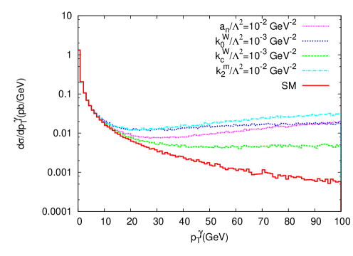
Figure 9: The $p_{T}$ distribution of the final state photon in $e^{+}e^{-}\to W^{-}W^{+}\gamma$ process with the anomalous $WWZ\gamma$ couplings $k_{0,c}^{W}/\Lambda^{2}$, $k_{2}^{m}/\Lambda^{2}$ and $a_{n}/\Lambda^{2}$ at $\sqrt{s}=0.5$ TeV.

The $p_{T}$ distribution of the final state photon in $e^{+}e^{-}\to W^{-}W^{+}\gamma$ process with the anomalous $WWZ\gamma$ couplings $\frac{k_{0}^{W}}{\Lambda^{2}}$, $\frac{k_{c}^{W}}{\Lambda^{2}}$, $\frac{k_{2}^{m}}{\Lambda^{2}}$ and $\frac{a_{n}}{\Lambda^{2}}$, together with SM backgrounds at $\sqrt{s}$=0.5, 1.5 and 3 TeV are given in Figs. $9$-$11$, respectively. From these figures, the final state photon in the $e^{+}e^{-}\to W^{-}W^{+}\gamma$ process is radiated from massless fermion-photon, $WW\gamma$ and $WWZ\gamma$ vertices. The massless fermion-photon vertex causes infrared singularities in the cross section. Therefore, the strong peak arises at the low $p_{T}$ region of the photons. Above $p_{T}$ of 20 GeV we see an obvious splitting and enhancement of the signal from SM background. The effects of infrared singularities which diminish the contribution of anomalous couplings to SM cross section become dominant for the high $p_{T}$ region, as shown in Fig. $9$-$11$. It is clear from Fig. 9 that the distributions are more sensitive to $\frac{k_{2}^{m}}{\Lambda^{2}}$ than to $\frac{a_{n}}{\Lambda^{2}}$. On the other hand, at $\sqrt{s}=$ 1.5 and 3 TeV, it shows exactly the opposite behavior. In addition, the momentum dependence of $\frac{k_{0}^{W}}{\Lambda^{2}}$ for all center of mass energies is bigger than $\frac{k_{c}^{W}}{\Lambda^{2}}$. Especially, the momentum dependence of $\frac{k_{0}^{W}}{\Lambda^{2}}$ between four different anomalous couplings is highest at $\sqrt{s}=$ 3 TeV. Consequently, we impose a $p_{T}>20$ GeV cut to reduce the SM background without affecting the signal cross sections due to anomalous quartic couplings.

In the course of statistical analysis, the limits of anomalous $\frac{k_{0}^{W}}{\Lambda^{2}}$, $\frac{k_{c}^{W}}{\Lambda^{2}}$, $\frac{k_{2}^{m}}{\Lambda^{2}}$ and $\frac{a_{n}}{\Lambda^{2}}$ couplings at $95\%$ C.L. are obtained by using $\chi^{2}$ test since the number of SM background events of the examined processes is greater than $10$. The $\chi^{2}$ function is defined as follows

$$\chi^{2}=\left(\frac{\sigma_{SM}-\sigma_{NP}}{\sigma_{SM}\delta_{stat}}\right)^{2}$$ (23)

where $\sigma_{NP}$ is the total cross section in the existence of anomalous gauge couplings, $\delta_{stat}=\frac{1}{\sqrt{N}}$ is the statistical error in which $N$ is the number of events. The number of expected events of the process $e^{+}e^{-}\rightarrow W^{-}W^{+}\gamma$, $N$ is obtained by $N=L_{int}\times\sigma_{SM}\times BR(W\rightarrow\ell\nu_{\ell})\times BR(W\rightarrow q\bar{q}^{\prime})$ where $L_{int}$ is the integrated luminosity, $\sigma_{SM}$ is the SM cross section and $\ell=e^{-}$ or $\mu^{-}$. Similarly, the number of expected events of the process $e^{+}e^{-}\rightarrow e^{+}\gamma^{*}e^{-}\rightarrow e^{+}W^{-}Z\nu_{e}$ is calculated as $N=L_{int}\times\sigma_{SM}\times BR(W\rightarrow\ell\nu_{\ell})\times BR(Z\rightarrow q\bar{q})$. In addition, we impose the acceptance cuts on the pseudorapidity $|\eta^{\,\gamma}|<2.5$ and the transverse momentum $p_{T}^{\,\gamma}>20\>$ GeV for photons in the process $e^{+}e^{-}\rightarrow W^{-}W^{+}\gamma$. After applying these cuts, the SM background cross sections for the process $e^{+}e^{-}\rightarrow W^{-}W^{+}\gamma$ are $1.65\times 10^{-1}$ pb at $\sqrt{s}=0.5$ TeV, $6.00\times 10^{-2}$ pb at $\sqrt{s}=1.5$ TeV, and $2.63\times 10^{-2}$ pb at $\sqrt{s}=3$ TeV. They are $3.58\times 10^{-3}$ pb at $\sqrt{s}=0.5$ TeV, $5.92\times 10^{-2}$ pb at $\sqrt{s}=1.5$ TeV, and $1.61\times 10^{-1}$ pb at $\sqrt{s}=3$ TeV for the process $e^{+}e^{-}\rightarrow e^{+}\gamma^{*}e^{-}\rightarrow e^{+}W^{-}Ze^{-}$.

The one-dimensional limits on anomalous couplings $\frac{k_{0}^{W}}{\Lambda^{2}}$, $\frac{k_{c}^{W}}{\Lambda^{2}}$, $\frac{k_{2}^{m}}{\Lambda^{2}}$ and $\frac{a_{n}}{\Lambda^{2}}$ at $95\%$ C.L. sensitivity at various integrated luminosities and center-of-mass energies are given in Tables I-VI. As can be seen in Tables I and II, the limits on $\frac{k_{0}^{W}}{\Lambda^{2}}$, $\frac{k_{c}^{W}}{\Lambda^{2}}$ are approximately several orders of magnitude more restrictive than those obtained from the LHC sınır while the best limits obtained on $\frac{a_{n}}{\Lambda^{2}}$ for the process $e^{+}e^{-}\rightarrow W^{-}W^{+}\gamma$ is five orders of magnitude more restrictive than those obtained from the LEP lep1 . In addition, as shown in Table III, we improve sensitivity to $\frac{k_{2}^{m}}{\Lambda^{2}}$ coupling with respect to limits derived by Ref. lhc1 , in which the best limits on this coupling in the literature are obtained. An important advantage of the examined $e^{+}e^{-}\rightarrow e^{+}\gamma^{*}e^{-}\rightarrow e^{+}W^{-}Z\nu_{e}$ process is that it isolates the anomalous $WWZ\gamma$ couplings, and therefore it enables us to examine $WWZ\gamma$ couplings independently from $WW\gamma\gamma$ couplings. In Table IV, the limits on the anomalous couplings $\frac{k_{0}^{W}}{\Lambda^{2}}$ and $\frac{k_{c}^{W}}{\Lambda^{2}}$ are obtained as $[-3.24;\,3.24]\times 10^{-7}$ and $[-4.71;\,4.70]\times 10^{-7}$ which can almost improve the sensitivities up to $37$ times for $\frac{k_{0}^{W}}{\Lambda^{2}}$ and $\frac{k_{c}^{W}}{\Lambda^{2}}$ with respect to LHC’s results. We show in Table V that the best limits on the anomalous coupling $\frac{a_{n}}{\Lambda^{2}}$ through the process $e^{+}e^{-}\rightarrow e^{+}\gamma^{*}e^{-}\rightarrow e^{+}W^{-}Z\nu_{e}$ are calculated as $[-1.17;\,1.17]\times 10^{-6}$ GeV^-2 which are more stringent than LEP’s results by almost five orders of magnitude. The best limits on $\frac{k_{2}^{m}}{\Lambda^{2}}$ via the process $e^{+}e^{-}\rightarrow e^{+}\gamma^{*}e^{-}\rightarrow e^{+}W^{-}Z\nu_{e}$ are $10$ times than the process $e^{+}e^{-}\rightarrow W^{-}W^{+}\gamma$ which improves the current experimental limits by a factor of $1.1$. In addition, we compare our limits with phenomenological studies on the anomalous couplings $\frac{k_{2}^{m}}{\Lambda^{2}}$ and $\frac{a_{n}}{\Lambda^{2}}$. Our limits on $\frac{k_{2}^{m}}{\Lambda^{2}}$ obtained from $e\gamma^{*}$ collision are 11 times more restrictive than the best limits obtained with the integrated luminosity of $200$ fb^-1 corresponding to $W^{\pm}Z\gamma$ production at the $14$ TeV LHC lhc1 . These limits are almost of the same order with our result obtained through the process $e^{+}e^{-}\rightarrow e^{+}\gamma^{*}e^{-}\rightarrow e^{+}W^{-}Z\nu_{e}$ at the CLIC with $L_{int}=100$ fb^-1 and $\sqrt{s}=1.5$ TeV. However, Ref. lin4 has considered incoming beam polarizations as well as the final state polarizations of the gauge bosons in the cross-section calculations to improve the bounds on anomalous $\frac{a_{n}}{\Lambda^{2}}$ coupling. We can see that the limits expected to be obtained for the future $\gamma\gamma$ colliders with $L_{int}=500$ fb^-1 and $\sqrt{s}=1.5$ TeV are $5$ times worse than our best limits when comparing to the unpolarized case. At the CLIC with $\sqrt{s}=3$ TeV for $L_{int}=590$ fb^-1, we can set more stringent limit by two orders of magnitude comparing to the limits on $\frac{a_{n}}{\Lambda^{2}}$ in Ref.lhc1 .

We show $95\%$ C.L. contours in the $\frac{k_{0}^{W}}{\Lambda^{2}}$-$\frac{k_{c}^{W}}{\Lambda^{2}}$ plane for the $e^{+}e^{-}\rightarrow W^{-}W^{+}\gamma$ process in Figs. $12$-$14$ for various integrated luminosity at $\sqrt{s}=0.5$ , 1 and 3 TeV, respectively. Similarly, the same contours for the process $e^{+}e^{-}\rightarrow e^{+}\gamma^{*}e^{-}\rightarrow e^{+}W^{-}Z\nu_{e}$ are depicted in Figs. $15$-$17$. As we can see from Fig. $14$, the best limits on anomalous couplings $\frac{k_{0}^{W}}{\Lambda^{2}}$ and $\frac{k_{c}^{W}}{\Lambda^{2}}$ are $[-1.90;1.92]\times 10^{-7}$ GeV^-2 and $[-3.34;3.29]\times 10^{-7}$ GeV^-2, respectively at $\sqrt{s}=3$ TeV for $L_{int}=590$ fb^-1. According to Fig. $17$, the attainable limits on $\frac{k_{0}^{W}}{\Lambda^{2}}$ and $\frac{k_{c}^{W}}{\Lambda^{2}}$ are $[-3.86;3.85]\times 10^{-7}$ GeV^-2 and $[-5.62;5.60]\times 10^{-7}$ GeV^-2, respectively.

III Conclusions

The CLIC is an proposed collider with energies on the TeV scale and extremely high luminosity. Particularly, operating with its high energy and luminosity is extremely important in order to investigate geniue anomalous $WWZ\gamma$ quartic gauge couplings that are described by dimension-six effective Lagrangians. Since energy dependences of the anomalous couplings are very high, the anomalous cross sections containing these couplings would have a higher momentum dependence than the SM cross section. We can easily understand that the contribution to the cross section of anomalous quartic couplings rapidly increases when the center-of-mass energy increases. Moreover, the geniue anomalous couplings can obtain higher sensitivity via analyzed reactions in the linear colliders due to very clean experimental conditions and being free from strong interactions with respect to LHC. Thus in this paper, we have examined CP-violating and CP-conserving Lagrangians for the anomalous $WWZ\gamma$ couplings in the processes $e^{+}e^{-}\rightarrow W^{-}W^{+}\gamma$ and $e^{+}e^{-}\rightarrow e^{+}\gamma^{*}e^{-}\rightarrow e^{+}W^{-}Z\nu_{e}$ at the CLIC. *

Appendix A The anomalous vertex functions for $WWZ\gamma$

The anomalous vertex for $W^{+}(p_{1}^{\alpha})W^{-}(p_{2}^{\beta})Z(k_{2}^{\nu})\gamma(k_{1}^{\mu})$ with the help of effective Lagrangian Eq. ($1$) is generated as follows

$$i\frac{\pi\alpha}{4\textmd{cos}\,\,\theta_{W}\Lambda^{2}}a_{n}[g_{\alpha\nu}[g_{\beta\mu}\,k_{1}.(k_{2}-p_{1})-k_{1\beta}.(k_{2}-p_{1})_{\mu}]$$

$$-g_{\beta\nu}[g_{\alpha\mu}\,k_{1}.(k_{2}-p_{2})-k_{1\alpha}.(k_{2}-p_{2})_{\mu}]$$

$$+g_{\alpha\beta}[g_{\nu\mu}k_{1}.(p_{1}-p_{2})-k_{1\nu}.(p_{1}-p_{2})_{\mu}]$$

$$-k_{2\alpha}(g_{\beta\mu}k_{1\nu}-g_{\nu\mu}k_{1\beta})+k_{2\beta}(g_{\alpha\mu}k_{1\nu}-g_{\nu\mu}k_{1\alpha})$$

$$-p_{2\nu}(g_{\alpha\mu}k_{1\beta}-g_{\beta\mu}k_{1\alpha})+p_{1\nu}(g_{\beta\mu}k_{1\alpha}-g_{\alpha\mu}k_{1\beta})$$

$$+p_{1\beta}(g_{\nu\mu}k_{1\alpha}-g_{\alpha\mu}k_{1\nu})+p_{2\alpha}(g_{\nu\mu}k_{1\beta}-g_{\beta\mu}k_{1\nu})].$$

In addition, the vertex functions for $W^{+}(p_{1}^{\alpha})W^{-}(p_{2}^{\beta})Z(k_{2}^{\nu})\gamma(k_{1}^{\mu})$ produced from the effective Lagrangians Eqs. ($8$)-($12$) are expressed below

$$2ie^{2}g^{2}g_{\alpha\beta}[g_{\mu\nu}(k_{1}.k_{2})-k_{1\nu}k_{2\mu}],$$ (25)

$$i\frac{e^{2}g^{2}}{2}[(g_{\mu\alpha}g_{\nu\beta}+g_{\nu\alpha}g_{\mu\beta})(k_{1}.k_{2})+g_{\mu\nu}(k_{2\beta}k_{1\alpha}+k_{1\beta}k_{2\alpha})$$

$$-k_{2\mu}k_{1\alpha}g_{\nu\beta}-k_{2\beta}k_{1\nu}g_{\mu\alpha}-k_{2\alpha}k_{1\nu}g_{\mu\beta}-k_{2\mu}k_{1\beta}g_{\nu\alpha}].$$ (26)

$$ieg_{z}g^{2}((g_{\mu\alpha}k_{1}.p_{1}-p_{1\mu}k_{1\alpha})g_{\nu\beta}+(g_{\mu\beta}k_{1}.p_{2}-p_{2\mu}k_{1\beta})g_{\nu\alpha})$$ (27)

$$i\frac{eg_{z}g^{2}}{2}((k_{1}.p_{1}+k_{1}.p_{2})g_{\mu\nu}g_{\alpha\beta}-(k_{1\alpha}p_{1\beta}+k_{1\beta}p_{2\alpha})g_{\mu\nu}$$

$$-(p_{1\mu}+p_{2\mu})k_{1\nu}g_{\alpha\beta}+(p_{1\beta}g_{\mu\alpha}+p_{2\alpha}g_{\mu\beta})k_{1\nu})$$ (28)

$$i\frac{eg_{z}g^{2}}{2}(k_{1}.p_{1}g_{\mu\beta}g_{\nu\alpha}+k_{1}.p_{2}g_{\mu\alpha}g_{\nu\beta}+(p_{1\nu}-p_{2\nu})k_{1\beta}g_{\mu\alpha}$$

$$-(p_{1\nu}-p_{2\nu})k_{1\alpha}g_{\mu\beta}-p_{1\mu}k_{1\beta}g_{\nu\alpha}-p_{2\mu}k_{1\alpha}g_{\nu\beta}).$$ (29)

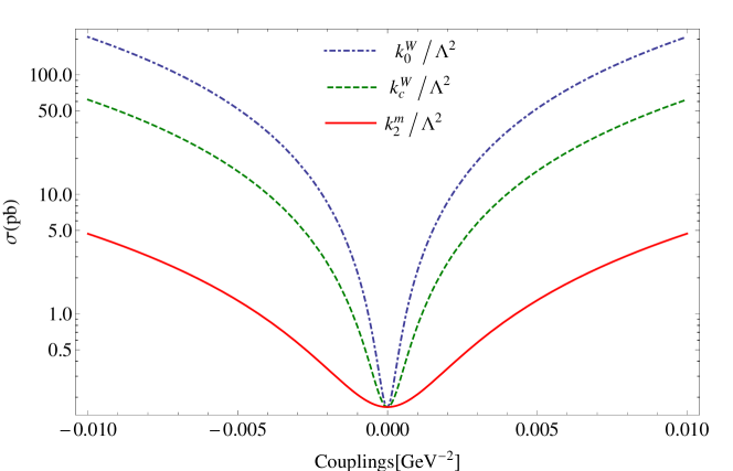
Figure 1: The total cross sections as function of anomalous $\frac{k_{0}^{W}}{\Lambda^{2}}$, $\frac{k_{c}^{W}}{\Lambda^{2}}$ and $\frac{k_{2}^{m}}{\Lambda^{2}}$ couplings for the $e^{+}e^{-}\rightarrow W^{-}W^{+}\gamma$ at the CLIC with $\sqrt{s}=0.5$ TeV.

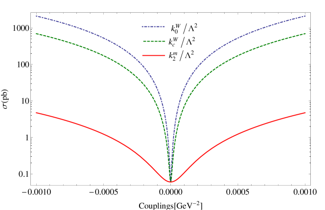
Figure 2: The same as Fig. 1 but for $\sqrt{s}=1.5$ TeV.

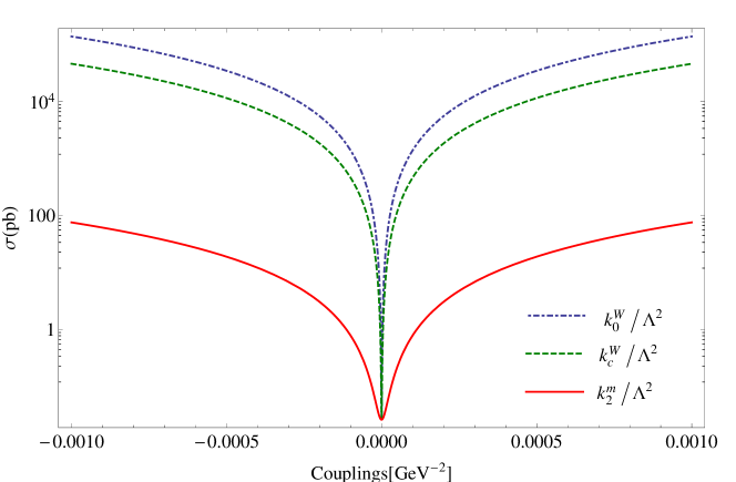
Figure 3: The same as Fig. 1 but for $\sqrt{s}=3$ TeV.

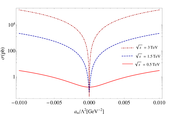
Figure 4: The total cross sections as function of anomalous $\frac{a_{n}}{\Lambda^{2}}$ coupling for the process $e^{+}e^{-}\rightarrow W^{-}W^{+}\gamma$ at the CLIC with $\sqrt{s}=0.5,1.5$ and $3$ TeV.

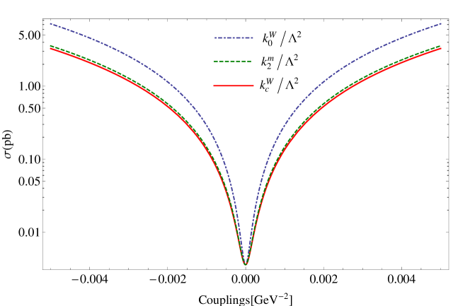
Figure 5: The total cross sections as function of anomalous $\frac{k_{0}^{W}}{\Lambda^{2}}$, $\frac{k_{c}^{W}}{\Lambda^{2}}$ and $\frac{k_{2}^{m}}{\Lambda^{2}}$ couplings for the process $e^{+}e^{-}\rightarrow e^{+}\gamma^{*}e^{-}\rightarrow e^{+}W^{-}Z\nu_{e}$ at the CLIC with $\sqrt{s}=0.5$ TeV.

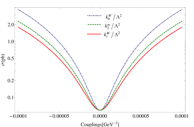
Figure 6: The same as Fig. 5 but for $\sqrt{s}=1.5$ TeV.

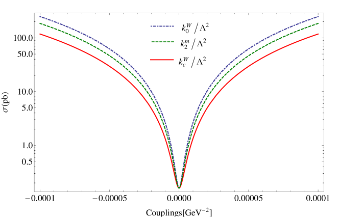
Figure 7: The same as Fig. 5 but for $\sqrt{s}=3$ TeV.

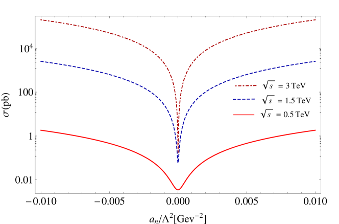
Figure 8: The total cross sections as function of anomalous $\frac{a_{n}}{\Lambda^{2}}$ coupling for the process $e^{+}e^{-}\rightarrow e^{+}\gamma^{*}e^{-}\rightarrow e^{+}W^{-}Z\nu_{e}$ at the CLIC with $\sqrt{s}=0.5,1.5$ and $3$ TeV.

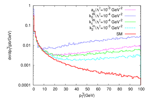
Figure 10: The same as Fig. 9 but for $\sqrt{s}=1.5$ TeV.

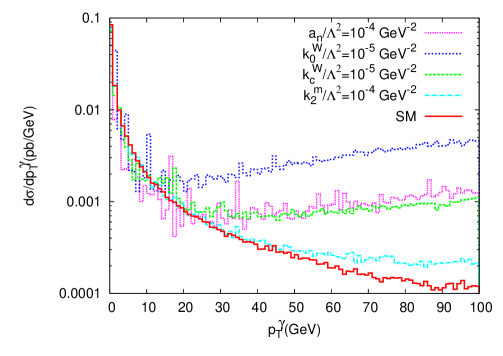
Figure 11: The same as Fig. 9 but for $\sqrt{s}=3$ TeV.

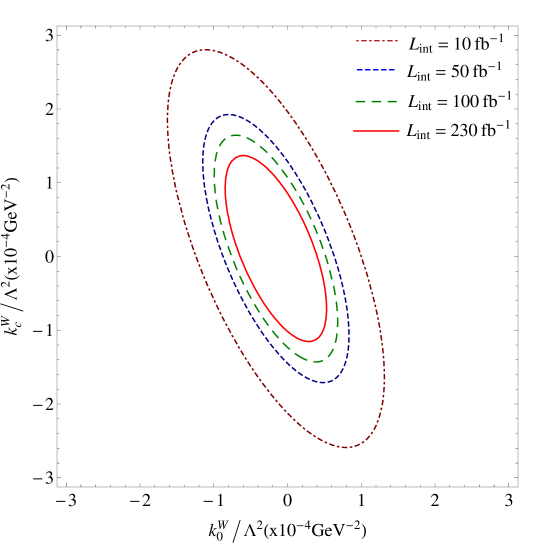
Figure 12: $95\%$ C.L. contours for anomalous $\frac{k_{0}^{W}}{\Lambda^{2}}$ and $\frac{k_{c}^{W}}{\Lambda^{2}}$ couplings for the process $e^{+}e^{-}\rightarrow W^{-}W^{+}\gamma$ at the CLIC with $\sqrt{s}=0.5$ TeV.

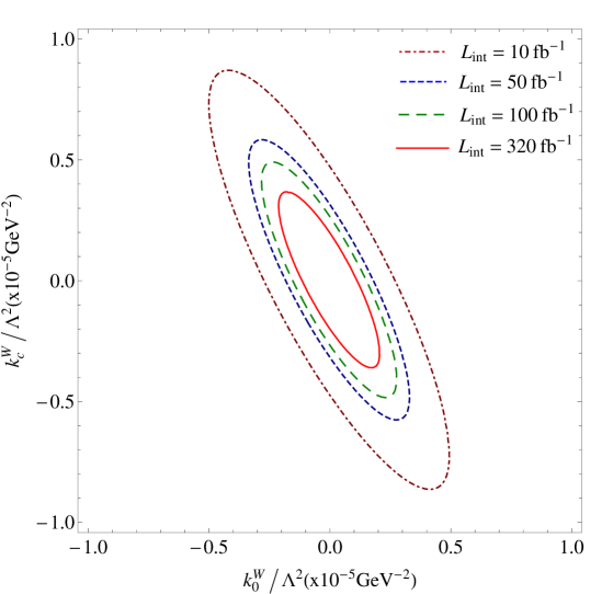
Figure 13: The same as Fig. 12 but for $\sqrt{s}=1.5$ TeV.

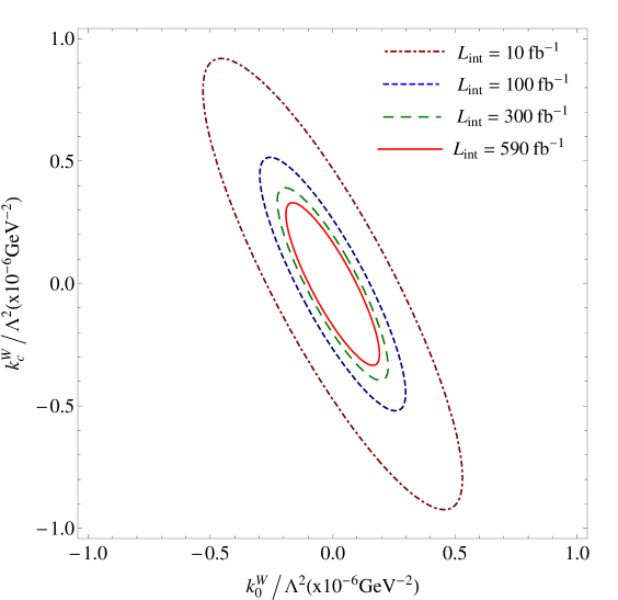
Figure 14: The same as Fig. 12 but for $\sqrt{s}=3$ TeV.

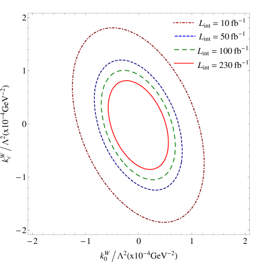
Figure 15: $95\%$ C.L. contours for anomalous $\frac{k_{0}^{W}}{\Lambda^{2}}$ and $\frac{k_{c}^{W}}{\Lambda^{2}}$ couplings for the process $e^{+}e^{-}\rightarrow e^{+}\gamma^{*}e^{-}\rightarrow e^{+}W^{-}Z\nu_{e}$ at the CLIC with $\sqrt{s}=0.5$ TeV.

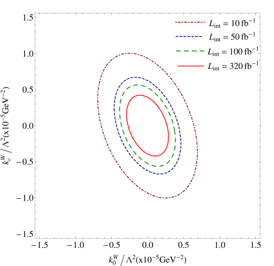
Figure 16: The same as Fig. 15 but for $\sqrt{s}=1.5$ TeV.

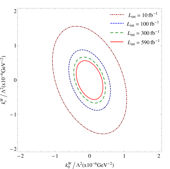
Figure 17: The same as Fig. 15 but for $\sqrt{s}=3$ TeV.

Table 1: $95\%$ C.L. sensitivity bounds of the $\frac{k_{0}^{W}}{\Lambda^{2}}$ and $\frac{k_{c}^{W}}{\Lambda^{2}}$ couplings through the process $e^{+}e^{-}\rightarrow W^{-}W^{+}\gamma$ at the CLIC with $\sqrt{s}=0.5,1.5$ and $3$ TeV.

$\sqrt{s}$ (TeV)	$L_{int}$(fb-1)	$\frac{k_{0}^{W}}{\Lambda^{2}}$(GeV-2)	$\frac{k_{c}^{W}}{\Lambda^{2}}$ (GeV-2)
$0.5$	$10$	$[-1.01;0.99]\times 10^{-4}$	$[-1.83;\,1.82]\times 10^{-4}$
$0.5$	$50$	$[-6.79;\,6.50]\times 10^{-5}$	$[-1.22;\,1.21]\times 10^{-4}$
$0.5$	$100$	$[-5.73;\,5.50]\times 10^{-5}$	$[-1.03;\,1.02]\times 10^{-4}$
$0.5$	$230$	$[-4.67;\,4.44]\times 10^{-5}$	$[-8.39;\,8.32]\times 10^{-5}$
$1.5$	$10$	$[-2.44;\,2.43]\times 10^{-6}$	$[-4.24;\,4.23]\times 10^{-6}$
$1.5$	$50$	$[-1.63;\,1.61]\times 10^{-6}$	$[-2.83;\,2.82]\times 10^{-6}$
$1.5$	$100$	$[-1.38;\,1.36]\times 10^{-6}$	$[-2.38;\,2.37]\times 10^{-6}$
$1.5$	$320$	$[-1.03;\,1.01]\times 10^{-6}$	$[-1.78;\,1.77]\times 10^{-6}$
$3$	$10$	$[-2.43;\,2.42]\times 10^{-7}$	$[-4.23;\,4.21]\times 10^{-7}$
$3$	$100$	$[-1.37;\,1.35]\times 10^{-7}$	$[-2.81;\,2.79]\times 10^{-7}$
$3$	$300$	$[-1.04;\,1.03]\times 10^{-7}$	$[-1.81;\,1.79]\times 10^{-7}$
$3$	$590$	$[-8.80;\,8.73]\times 10^{-8}$	$[-1.53;\,1.51]\times 10^{-7}$

Table 2: $95\%$ C.L. sensitivity bounds of the $\frac{a_{n}}{\Lambda^{2}}$ couplings through the process $e^{+}e^{-}\rightarrow W^{-}W^{+}\gamma$ at the CLIC with $\sqrt{s}=0.5,1.5$ and $3$ TeV.

$\sqrt{s}$ (TeV)	$L_{int}$(fb-1)	$\frac{a_{n}}{\Lambda^{2}}$ (GeV-2)
$0.5$	$10$	$[-8.47;\,8.45]\times 10^{-4}$
$0.5$	$50$	$[-5.67;\,5.65]\times 10^{-4}$
$0.5$	$100$	$[-4.77;\,4.75]\times 10^{-4}$
$0.5$	$230$	$[-3.88;\,3.85]\times 10^{-4}$
$1.5$	$10$	$[-2.59;\,2.57]\times 10^{-5}$
$1.5$	$50$	$[-1.85;\,1.83]\times 10^{-5}$
$1.5$	$100$	$[-1.63;\,1.61]\times 10^{-5}$
$1.5$	$320$	$[-1.35;\,1.33]\times 10^{-5}$
$3$	$10$	$[-2.46;\,2.46]\times 10^{-6}$
$3$	$100$	$[-1.38;\,1.38]\times 10^{-6}$
$3$	$300$	$[-1.05;\,1.05]\times 10^{-6}$
$3$	$590$	$[-9.13;\,9.09]\times 10^{-7}$

Table 3: $95\%$ C.L. sensitivity bounds of the $\frac{k_{2}^{m}}{\Lambda^{2}}$ couplings through the process $e^{+}e^{-}\rightarrow W^{-}W^{+}\gamma$ at the CLIC with $\sqrt{s}=0.5,1.5$ and $3$ TeV.

$\sqrt{s}$ (TeV)	$L_{int}$(fb-1)	$\frac{k_{2}^{m}}{\Lambda^{2}}$(GeV-2)
$0.5$	$10$	$[-6.87;\,6.68]\times 10^{-4}$
$0.5$	$50$	$[-4.62;\,4.43]\times 10^{-4}$
$0.5$	$100$	$[-3.90;\,3.72]\times 10^{-4}$
$0.5$	$230$	$[-3.19;\,3.00]\times 10^{-4}$
$1.5$	$10$	$[-5.17;\,5.15]\times 10^{-5}$
$1.5$	$50$	$[-3.46;\,3.44]\times 10^{-5}$
$1.5$	$100$	$[-2.91;\,2.89]\times 10^{-5}$
$1.5$	$320$	$[-2.18;\,2.16]\times 10^{-5}$
$3$	$10$	$[-1.05;\,1.03]\times 10^{-5}$
$3$	$100$	$[-5.92;\,5.79]\times 10^{-6}$
$3$	$300$	$[-4.51;\,4.38]\times 10^{-6}$
$3$	$590$	$[-3.82;\,3.69]\times 10^{-6}$

Table 4: $95\%$ C.L. sensitivity bounds of the $\frac{k_{0}^{W}}{\Lambda^{2}}$ and $\frac{k_{c}^{W}}{\Lambda^{2}}$ couplings through the processes $e^{+}e^{-}\rightarrow e^{+}\gamma^{*}e^{-}\rightarrow e^{+}W^{-}Z\nu_{e}$ at the CLIC with $\sqrt{s}=0.5,1.5$ and $3$ TeV.

$\sqrt{s}$ (TeV)	$L_{int}$(fb-1)	$\frac{k_{0}^{W}}{\Lambda^{2}}$(GeV-2)	$\frac{k_{c}^{W}}{\Lambda^{2}}$ (GeV-2)
$0.5$	$10$	$[-1.03;\,1.01]\times 10^{-4}$	$[-1.53;\,1.48]\times 10^{-4}$
$0.5$	$50$	$[-6.97;\,6.69]\times 10^{-5}$	$[-1.04;\,0.98]\times 10^{-4}$
$0.5$	$100$	$[-5.88;\,5.60]\times 10^{-5}$	$[-8.75;\,8.22]\times 10^{-5}$
$0.5$	$230$	$[-4.80;\,4.52]\times 10^{-5}$	$[-7.16;\,6.62]\times 10^{-5}$
$1.5$	$10$	$[-5.76;\,5.75]\times 10^{-6}$	$[-8.37;\,8.35]\times 10^{-6}$
$1.5$	$50$	$[-3.86;\,3.85]\times 10^{-6}$	$[-5.60;\,5.58]\times 10^{-6}$
$1.5$	$100$	$[-3.24;\,3.23]\times 10^{-6}$	$[-4.71;\,4.69]\times 10^{-6}$
$1.5$	$320$	$[-2.43;\,2.42]\times 10^{-6}$	$[-3.53;\,3.50]\times 10^{-6}$
$3$	$10$	$[-8.98;\,8.97]\times 10^{-7}$	$[-1.31;\,1.30]\times 10^{-6}$
$3$	$100$	$[-5.05;\,5.04]\times 10^{-7}$	$[-7.34;\,7.33]\times 10^{-7}$
$3$	$300$	$[-3.84;\,3.83]\times 10^{-7}$	$[-5.58;\,5.57]\times 10^{-7}$
$3$	$590$	$[-3.24;\,3.24]\times 10^{-7}$	$[-4.71;\,4.70]\times 10^{-7}$

Table 5: $95\%$ C.L. sensitivity bounds of the $\frac{a_{n}}{\Lambda^{2}}$ couplings through the processes $e^{+}e^{-}\rightarrow e^{+}\gamma^{*}e^{-}\rightarrow e^{+}W^{-}Z\nu_{e}$ at the CLIC with $\sqrt{s}=0.5,1.5$ and $3$ TeV.

$\sqrt{s}$ (TeV)	$L_{int}$(fb-1)	$\frac{a_{n}}{\Lambda^{2}}$ (GeV-2)
$0.5$	$10$	$[-4.08;\,3.96]\times 10^{-4}$
$0.5$	$50$	$[-2.75;\,2.63]\times 10^{-4}$
$0.5$	$100$	$[-2.33;\,2.20]\times 10^{-4}$
$0.5$	$230$	$[-1.90;\,1.78]\times 10^{-4}$
$1.5$	$10$	$[-2.19;\,2.17]\times 10^{-5}$
$1.5$	$50$	$[-1.47;\,1.45]\times 10^{-5}$
$1.5$	$100$	$[-1.23;\,1.22]\times 10^{-5}$
$1.5$	$320$	$[-9.26;\,9.07]\times 10^{-6}$
$3$	$10$	$[-3.16;\,3.16]\times 10^{-6}$
$3$	$100$	$[-1.78;\,1.77]\times 10^{-6}$
$3$	$300$	$[-1.35;\,1.35]\times 10^{-6}$
$3$	$590$	$[-1.17;\,1.17]\times 10^{-6}$

Table 6: $95\%$ C.L. sensitivity bounds of the $\frac{k_{2}^{m}}{\Lambda^{2}}$ couplings through the processes $e^{+}e^{-}\rightarrow e^{+}\gamma^{*}e^{-}\rightarrow e^{+}W^{-}Z\nu_{e}$ at the CLIC with $\sqrt{s}=0.5,1.5$ and $3$ TeV.

$\sqrt{s}$ (TeV)	$L_{int}$(fb-1)	$\frac{k_{2}^{m}}{\Lambda^{2}}$(GeV-2)
$0.5$	$10$	$[-1.48;\,1.41]\times 10^{-4}$
$0.5$	$50$	$[-9.98;\,9.36]\times 10^{-5}$
$0.5$	$100$	$[-8.45;\,7.42]\times 10^{-5}$
$0.5$	$230$	$[-6.92;\,6.29]\times 10^{-5}$
$1.5$	$10$	$[-7.38;\,7.37]\times 10^{-6}$
$1.5$	$50$	$[-4.94;\,4.92]\times 10^{-6}$
$1.5$	$100$	$[-4.15;\,4.14]\times 10^{-6}$
$1.5$	$320$	$[-3.11;\,3.09]\times 10^{-6}$
$3$	$10$	$[-1.04;\,1.04]\times 10^{-6}$
$3$	$100$	$[-5.85;\,5.84]\times 10^{-7}$
$3$	$300$	$[-4.44;\,4.43]\times 10^{-7}$
$3$	$590$	$[-3.75;\,3.74]\times 10^{-7}$