Neutrino Emission in Jet Propagation Process

Abstract

Relativistic jets are universal in long-duration gamma-ray burst (GRB) models. Before breaking out, they must propagate in the progenitor envelope along with a forward shock and a reverse shock forming at the jet head. Both electrons and protons will be accelerated by the shocks. High energy neutrinos could be produced by these protons interacting with stellar materials and electron-radiating photons. The jet will probably be collimated, which may have a strong effect on the final neutrino flux. Under the assumption of a power-law stellar-envelope density profile $\rho\propto r^{-\alpha}$ with an index $\alpha$, we calculate this neutrino emission flux by these shocks for low-luminosity GRBs (LL-GRBs) and ultra-long GRBs (UL-GRBs) in different collimation regimes, using the jet propagation framework developed by Bromberg et al. (2011). We find that LL-GRBs and UL-GRBs are capable for detectable high energy neutrinos up to $\sim{\rm PeV}$, and obtain the final neutrino spectrum. Besides, we conclude that larger $\alpha$ corresponds to greater neutrino flux at high energy end ($\sim{\rm PeV}$) and higher maximum neutrino energy as well. However, such differences are so small that it is not promising for us to distinguish from observations, given the energy resolution we have now.

1 Introduction

The collapsar model of gamma-ray bursts suggests that during the core collapse of a progenitor massive star to a neutron star or a black hole, a relativistic jet punctures the stellar envelope and transports energy to electrons and protons through shock acceleration (Zhang & Mészáros, 2004; Piran, 2005; Mészáros, 2006; Woosley, 1993; MacFadyen & Woosley, 1999). Accelerated electrons dominate radiation via synchrotron or inverse Compton mechanism while accelerated protons produce neutrinos by proton-proton collision and photopion process (Waxman & Bahcall, 1997, 1999; Rachen & Mészáros, 1998; Alvarez-Muniz et al., 2000; Bahcall & Waxman, 2001; Guetta & Granot, 2003; Murase et al., 2006; Becker, 2008). Within this scenario, we can expect high energy neutrinos originating from different stages in a GRB event. First, Waxman & Bahcall (2000) and Dai & Lu (2001) proposed $\epsilon_{\nu}>10^{3}\,{\rm TeV}$ neutrinos from an external reverse shock. Similarly, neutrinos from an external forward shock have been discussed (Li et al., 2002; Dermer et al., 2003; Razzaque, 2013). Second, the prompt photon emission from GRBs can be correlated to the production of neutrinos, since protons are also believed to be accelerated in relativistic internal shocks (Vietri, 1995; Waxman & Bahcall, 1997, 1999; Mészáros & Rees, 2000; Guetta et al., 2004). Murase & Nagataki (2006) obtained a diffuse neutrino background spectrum from GRBs for specific parameter sets in the internal shock model. Alternatively, the neutrino emission might arise in a dissipative jet photosphere (Rees & Mészáros, 2005; Murase, 2008; Wang & Dai, 2009; Gao et al., 2012). Third, neutrinos could also be produced while the jet is still propagating in the envelope. Generally, these neutrinos appear as a precursor burst. Mészáros & Waxman (2001) predicted a neutrino precursor of $\epsilon_{\nu}\geq 5\,{\rm TeV}$, which is produced by internal shocks at radius $r_{\rm IS}\approx 10^{10}-10^{11}\,{\rm cm}$. Enberg et al. (2009) presented a new analysis of the neutrino flux of these internal shocks for two types of source environments: the slow-jet supernova (SJS) model and the GRB model. Still further, Murase & Ioka (2013) studied high energy neutrino production in collimated jets inside progenitors of gamma-ray bursts and supernovae, considering both collimation and internal shocks. Pruet (2003) discussed the neutrinos produced by inelastic neutron-nucleon collisions of a relativistic jet propagating through a stellar envelope. Razzaque et al. (2003) dealt with the high energy neutrino signature in a supernova remnant shell ejected prior to a gamma-ray burst and then Ando & Beacom (2005) extended their model and significantly improved the detection prospects. Horiuchi & Ando (2008) proposed that a reverse shock at the jet head probably will accelerate protons when crossing the jet material, and they calculated in detail the cumulative neutrino event number that may be observed by a ${\rm km}^{2}$ scale detector like IceCube.

The jet propagation dynamics has been studied. Assuming a constant jet velocity, Begelman & Cioffi (1989) discussed the propagation of a galactic jet in the intergalactic medium. Mészáros & Waxman (2001) analyzed the propagation in the envelope of a red supergiant star, ignoring the surrounding cocoon. Matzner (2003) studied the jet-cocoon structure and jet head velocity that is constrained by ram pressure balance, but they did not consider the collimation by cocoon pressure. Lazzati & Begelman (2005) took into account the collimation effect and meanwhile they assumed that the jet expands adiabatically. Bromberg et al. (2011) considered a collimated shock that forms at the base of the jet and dissipates parts of the jet’s energy to counterbalance the cocoon’s pressure. They figured out the geometry of a collimated shock, and thus further obtained the requirement for jet collimation. Moreover, it is worth mentioning that various numerical simulations of jet propagation in the envelope already have been performed (Zhang et al., 2003; Morsony et al., 2007; Mizuta & Aloy, 2009; Mizuta & Ioka, 2013).

In our paper we try to calculate the flux of high energy neutrinos from the shocks formed at the jet head for low-luminosity GRBs (LL-GRBs) and ultra-long GRBs (UL-GRBs), when the jet is still propagating inside the envelope. Most importantly, we take into account the jet collimation which could largely affect the final neutrino flux but was ignored in the previous studies. For simplicity, we only account for jet propagation in the helium core because collimation mainly happens there. We assume a power law envelope density profile $\rho(r)=Ar^{-\alpha}$, where $A=(3-\alpha)M_{\rm He}/(4\pi r_{\rm He}^{3-\alpha})$ and $2\leq\alpha<3$ with $M_{\rm He}$ and $r_{\rm He}$ being the mass and radius of the helium envelope. We employ the analytical solutions described in Bromberg et al. (2011) to further calculate the neutrino flux in different collimation regimes and at last we discuss its dependence on the index $\alpha$, providing an alternative way to probe the GRB progenitor through neutrino precursor signal in the future.

This paper is organized as follows. In section 2 we discuss the jet propagation dynamics. In section 3 we perform detailed calculations of neutrino flux in each regime and a comparison between different regimes. Dependence on $\alpha$ is considered in section 4. We make a comparison with previous works in Section 5 and finally we finish with discussions and conclusions in section 6.

2 Jet Propagation Dynamics

According to Matzner (2003), the head velocity is constrained by ram pressure balance,

$$\rho_{j}h_{j}\Gamma_{j}^{2}\Gamma_{h}^{2}(\beta_{j}-\beta_{h})^{2}+P_{j}=\rho_{a}h_{a}\Gamma_{h}^{2}\beta_{h}^{2}+P_{a},$$

where $\rho,P,\beta,\Gamma$ and $h\equiv 1+4P/\rho c^{2}$ are the density, pressure, velocity, Lorentz factor and dimensionless specific enthalpy, and the subscripts $j$ and $a$ refer to jet and ambient material. Then the jet head velocity is

$$\beta_{h}=\frac{\beta_{j}}{1+\tilde{L}^{-1/2}},$$

with

$$\tilde{L}\equiv\frac{\rho_{j}h_{j}\Gamma_{j}^{2}}{\rho_{a}}\simeq\frac{L_{j}}{\Sigma_{j}\rho_{a}c^{3}},$$

where $L_{j}$ is the jet luminosity and $\Sigma_{j}=\pi r_{j}^{2}$ is the jet’s cross section.

The parameter $\tilde{L}$ is crucial for determining collimation regimes (see Bromberg et al., 2011, Table 1). While $\tilde{L}\lesssim\theta_{0}^{-4/3}$ the jet is strongly collimated by the cocoon pressure, where $\theta_{0}$ is the jet opening angle. Bromberg et al. (2011) would further divide it into two situations: $\tilde{L}\ll 1$ and $1\ll\tilde{L}\lesssim\theta_{0}^{-4/3}$. The uncollimated regime corresponds to $\tilde{L}>\theta_{0}^{-4/3}$, accordingly.

The internal energy and particle number density of the shocked and unshocked regions are correlated by (Blandford & McKee, 1976; Sari & Piran, 1995)

$$\frac{e_{f}}{n_{f}m_{p}c^{2}}=\Gamma_{h}-1,\quad\frac{n_{f}}{n_{a}}=4\Gamma_{h}+3,$$

$$\frac{e_{r}}{n_{r}m_{p}c^{2}}=\bar{\Gamma}_{h}-1,\quad\frac{n_{r}}{n_{j}}=4\bar{\Gamma}_{h}+3,$$

where the subscripts $f$ and $r$ represent regions that have been crossed by the forward shock and reverse shock. $\Gamma_{h}$ is the Lorentz factor of the head and $\bar{\Gamma}_{h}$ is the Lorentz factor of the unshocked jet measured in the jet head frame,

$$\bar{\Gamma}_{h}=\Gamma_{j}\Gamma_{h}(1-\beta_{j}\beta_{h}).$$

Moreover, the density of the unshocked jet materials $\rho_{j}$ is determined by

$$L_{j}=\Gamma_{j}^{2}\pi r_{j}^{2}\rho_{j}c^{3}.$$

Based on the above equations, we can carry on our calculation.

3 Theoretical Calculation of Neutrino Flux

In this section, we take $\alpha=2$ as our premise, and discuss the dependence on $\alpha$ later in section 4.

The most promising acceleration process in a GRB is Fermi acceleration mechanism. But now there are noteworthy arguments that once the the jet bulk kinetic energy is dissipated at the collimation shock, the collimated jet would become radiation dominated and then the reverse shock occurring at the interface of the jet head and collimated jet would also be radiation mediated. At such shocks, photons produced in the downstream diffuse into the upstream and interact with electrons or pairs. There would not be a strong shock jump any more and Fermi acceleration no longer works (Levinson & Bromberg, 2008; Katz et al., 2010; Murase & Ioka, 2013). However, this case is changed for LL-GRBs (Soderberg et al., 2006; Toma et al., 2007; Liang et al., 2007; Murase & Ioka, 2013) and UL-GRBs (Levan et al., 2013; Gendre et al., 2013; Murase & Ioka, 2013). Because of low power or large radii, the Thomson optical depth is low even inside a star (Murase & Ioka, 2013) so that efficient Fermi acceleration would be expected. We consider LL-GRBs and UL-GRBs separately and they fall into different collimation regimes, which will be talked about later.

Due to the first order Fermi acceleration, the accelerated proton spectrum is (Achterberg et al., 2001; Keshet & Waxman, 2005; Horiuchi & Ando, 2008):

$$\frac{{\rm d}n_{p}}{{\rm d}\epsilon_{p}}\propto\epsilon_{p}^{-p},$$

where $\epsilon_{p}$ and $n_{p}$ are the proton energy and number density. We optimistically take $p=2$ in our calculation. The minimum proton energy $\epsilon_{p,\min}\sim\Gamma_{j}m_{p}c^{2}$ and maximum energy $\epsilon_{p,\max}$ is determined by the balance between proton acceleration and cooling process.

3.1 $\tilde{L}\ll 1$

In this regime, the jet head moves forward with a non-relativistic velocity, $\Gamma_{h}\simeq 1$. The unshocked jet’s Lorentz factor in the head frame is $\bar{\Gamma}_{h}=\Gamma_{j}$. We can easily see that the reverse shock is strong while the forward shock is so weak that we need not consider. The internal energy of the shocked jet is $e_{r}\simeq(\Gamma_{j}-1)(4\Gamma_{j}+3)\rho_{j}c^{2}$. In addition, we deduce some crucial terms below analytically (see Bromberg et al., 2011, Appendix B).

$$\tilde{L}=\left(\frac{16}{\pi}\right)^{2/3}L_{j}^{2/3}A^{-2/3}\theta_{0}^{-8/3}c^{-2},$$

$$\theta_{j}=2^{-4/3}\pi^{-1/6}L_{j}^{1/6}A^{-1/6}\theta_{0}^{8/15}c^{-1/2},$$

$$\rho_{j}=2^{8/3}\pi^{-2/3}\Gamma_{j}^{-2}L_{j}^{2/3}A^{1/3}r^{-2}\theta_{0}^{-16/15}c^{-2},$$

where $\theta_{0}$ is the initial jet opening angle and $\theta_{j}$ is the opening angle after collimation. Fortunately, $\tilde{L},\theta_{j}$ do not vary with radius when and only when $\alpha=2$.

The internal energy

$$e_{r}=2^{8/3}\pi^{-2/3}\frac{(4\Gamma_{j}+3)(\Gamma_{j}-1)}{\Gamma_{j}^{2}}L_{j}^{2/3}A^{1/3}r^{-2}\theta_{0}^{-16/15}.$$

We assume the energy equipartition factor $\varepsilon_{e}=\varepsilon_{B}=0.1$ and thus we can get the comoving magnetic field by

$$\frac{B^{2}}{8\pi}=\varepsilon_{B}e_{r},$$

$$B=2^{17/6}\pi^{1/6}\sqrt{\varepsilon_{B}\frac{(4\Gamma_{j}+3)(\Gamma_{j}-1)}{\Gamma_{j}^{2}}}L_{j}^{1/3}A^{1/6}r^{-1}\theta_{0}^{-8/15}.$$

Because of the large opacity of the envelope, the radiation of relativistic electrons will be thermalized, with a typical black body temperature

$$\frac{8\pi^{5}(kT)^{4}}{15(hc)^{3}}=\varepsilon_{e}e_{r},$$

$$kT=2^{2/3}\pi^{-1/6}[\frac{15\varepsilon_{e}(hc)^{3}}{8\pi^{5}}\frac{(4\Gamma_{j}+3)(\Gamma_{j}-1)}{\Gamma_{j}^{2}}]^{1/4}L_{j}^{1/6}A^{1/12}r^{-1/2}\theta_{0}^{-4/15}.$$

The average number density of thermal photons is

$$n_{\gamma}=19.232\pi\times\frac{1}{(hc)^{3}}\times(kT)^{3}.$$

Furthermore, in order to get the numerical values, we adopt the typical values of LL-GRBs, $L_{\rm iso}=10^{46}{\rm erg\,s}^{-1}$, $\theta_{0}=0.02$, which suggests $L_{j}=10^{42}{\rm erg\,s}^{-1}$. So the Lorentz factor of collimated jet is $\Gamma_{j}\sim 1/\theta_{0}\sim 50$(Mizuta & Ioka, 2013). According to Heger et al. (2000) and Woosley & Heger (2006), we assume a typical progenitor with a helium core of mass $\sim 2M_{\odot}$ and radius $r_{\rm He}=4\times 10^{11}\,$cm so that the ambient envelope density can be expressed as $\rho_{a}(r)=7.96\times 10^{20}r^{-2}\;{\rm g\,cm}^{-3}$. From equation (8) we get $\tilde{L}\simeq 0.013\;,\;\rho_{j}=4.95\times 10^{-11}\;{\rm g\,cm}^{-3}$ so that this LL-GRB meets the requirement $\tilde{L}\ll 1$. Moreover, Fermi acceleration is efficient because the Thomson optical depth is $\tau_{T}=n\sigma_{T}l=\frac{\rho_{j}}{m_{p}}\sigma_{T}\frac{r_{\rm He}}{\Gamma_{j}}\simeq 0.158(\frac{L_{j}}{10^{42}{\rm erg\,s}^{-1}})^{\frac{2}{3}}(\frac{\theta_{0}}{0.02})^{\frac{29}{15}}(\frac{M_{\rm He}}{2M_{\odot}})^{\frac{1}{3}}(\frac{r_{\rm He}}{4\times 10^{11}\rm cm})^{-\frac{4}{3}}\sim 0.1C^{-1}\bar{\Gamma}_{h}<1$, where $C=1+2\ln\bar{\Gamma}_{h}^{2}$ is the possible effect by pair production (Murase & Ioka, 2013; Budnik et al., 2010; Nakar & Sari, 2012). Now we can get $B=3.33\times 10^{7}$G, $kT=0.76\,{\rm keV}$, $n_{\gamma}=1.36\times 10^{22}{\rm cm}^{-3}$. Remember that this is measured in the rest frame of the jet head.

A high energy proton loses its energy through radiative and hadronic process. The radiative cooling includes synchrotron and inverse Compton scattering, with typical cooling timescales (Horiuchi & Ando, 2008):

$$t_{\rm sync}=\frac{6\pi m_{p}^{4}c^{3}}{\sigma_{T}m_{e}^{2}B^{2}\epsilon_{p}},$$

$$t_{\rm IC,Th}=\frac{3m_{p}^{4}c^{3}}{4\sigma_{T}m_{e}^{2}\epsilon_{\gamma}n_{\gamma}\epsilon_{p}},$$

$$t_{\rm IC,KN}=\frac{3\epsilon_{\gamma}\epsilon_{p}}{4\sigma_{T}m_{e}^{2}c^{5}n_{\gamma}},$$

where the subscripts ${\rm Th,KN}$ represent the Thomson limit and Klein-Nishina limit of inverse Compton scattering, $\sigma_{T}$ is the Thomson cross section and average photon energy $\bar{\epsilon}_{\gamma}=2.7kT$. If the proton energy $\epsilon_{p}$ is in units of GeV, the numerical values of the timescales given above are

$$t_{\rm sync}=t_{\rm IC,Th}=4.07\times 10^{3}\frac{1}{\epsilon_{p}}\;{\rm s},\;\;\;t_{\rm IC,KN}=2.16\times 10^{-8}\epsilon_{p}\;{\rm s}.$$

Hadronic cooling mechanisms mainly contain proton-proton collision, the Bethe-Heitler interaction and photopion production in the following ways respectively,

$$p+p\longrightarrow\pi^{\pm},K^{\pm}\longrightarrow\mu^{\pm}+\nu_{\mu}(\bar{\nu}_{\mu}),$$

$$p+\gamma\longrightarrow p+e^{\pm},$$

$$p+\gamma\longrightarrow p+\pi^{0}\quad{\rm or}\quad p+\gamma\longrightarrow n+\pi^{+}.$$

We can expect muon neutrinos to be produced in pp and photopion process, via charged pion or kaon decay. Here we do not consider the secondary electron neutrino production.

The cooling timescale of pp collision is

$$t_{pp}=\frac{\epsilon_{p}}{c\sigma_{pp}n_{p}\Delta{\epsilon_{p}}}.$$

We estimate the proton number density in the shocked jet as $n_{p}=(4\Gamma_{j}+3)\rho_{j}/m_{p}\sim 6.02\times 10^{15}{\rm cm}^{-3}$. Assuming in each collision a fraction 20% of the proton energy is lost and $\sigma_{pp}=5\times 10^{-26}{\rm cm}^{2}$ (Eidelman et al., 2004), we can get $t_{pp}=0.55\,{\rm s}$.

At relative higher energy, the protons start to cool through the Bethe-Heiter interaction, for which the energy loss every times is $\Delta{\epsilon_{p}}=2m_{e}c^{2}\gamma_{\rm c.m.}$, where $\gamma_{\rm c.m.}$ is the Lorentz factor of the center of inertia in the comoving frame and can be expressed as $\gamma_{\rm c.m.}=(\epsilon_{p}+\epsilon_{\gamma})/(m_{p}^{2}c^{4}+2\epsilon_{p}\epsilon_{\gamma})^{1/2}$. The BH cross section is given by $\sigma_{\rm BH}=(28/9)\alpha r_{e}^{2}\ln[(2\epsilon_{p}\epsilon_{\gamma})/(m_{p}m_{e}c^{4})-106/9]$, so the BH cooling time is (Razzaque et al., 2004; Horiuchi & Ando, 2008)

$$t_{\rm BH}=\frac{\epsilon_{p}}{2n_{\gamma}c\sigma_{\rm BH}m_{e}c^{2}\gamma_{\rm c.m.}}.$$

The photopion production dominates the cooling even at higher energy. We adopt the photopion cross section described in Stecker (1968) and Asano (2005) as a broken power law: $\sigma(\chi)=5\times 10^{-28}(\chi/590)^{3.2}{\rm cm}^{2}$ for $290<\chi<590$ and $\sigma(\chi)=5\times 10^{-28}(\chi/590)^{-0.7}{\rm cm}^{2}$ for $590<\chi<9800$, where $\chi m_{e}c^{2}$ is the photon energy in the proton rest frame. Thus the cooling timescale is

$$t_{p\gamma}=\frac{\epsilon_{p}}{c\sigma_{p\gamma}n_{\gamma}\Delta{\epsilon_{p}}},$$

where the conventional inelasticity $K=\Delta{\epsilon_{p}}/\epsilon_{p}=[1-(m_{p}^{2}-m_{\pi}^{2})/s]/2$ and $s$ is the invariant mass of the system.

The timescale of the first order Fermi acceleration is $t_{\rm acc}=\theta_{F}\epsilon_{p}/(eBc)$. If the diffusion coefficient is assumed to be proportional to the Bohm diffusion coefficient and $\theta_{F}$ is taken to be the common value $\theta_{F}=10$ (Razzaque et al., 2004; Ando et al., 2005; Horiuchi & Ando, 2008), then $t_{\rm acc}\sim 3.32\times 10^{-11}\epsilon_{p}\,{\rm s}$.

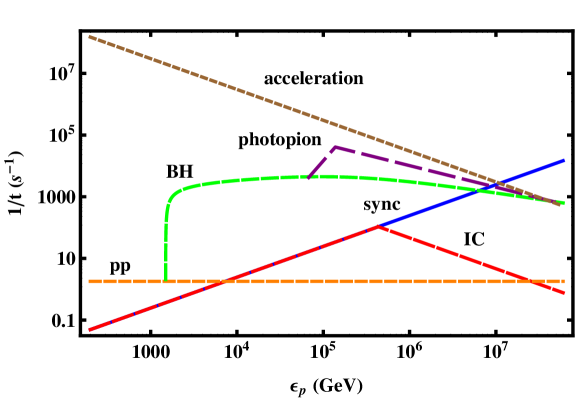
Figure 1: Inverse of proton cooling and acceleration timescales (brown short dashed) versus proton energy, in the jet head rest frame. Cooling mechanisms are synchrotron (blue solid), inverse Compton (red long dashed), proton proton collision (orange dashed), Bethe-Heitler (green dashed) and photopion process (purple dashed). Relevant parameters: $L_{j}=10^{42}{\rm erg\,s}^{-1}$, $\theta_{0}=0.02$, $r_{\rm He}=4\times 10^{11}{\rm cm}$, $\epsilon_{e}=\epsilon_{B}=0.1$.

We now can plot the inverse of all these timescales as functions of proton energy in Figure 1. The maximum proton energy can be obtained by $t_{\rm sync}=t_{\rm acc}$, so $\epsilon_{p,\max}\simeq 1.11\times 10^{7}{\rm GeV}$. Hence we expect the maximum neutrino energy produced by this LL-GRB as $\epsilon_{\nu,\max}\simeq\frac{1}{10}\epsilon_{p,\max}\simeq 1.11{\rm PeV}$.

We can define two threshold proton energies $\epsilon_{p,\rm th}^{({\rm BH})}$ and $\epsilon_{p,\rm th}^{(p\gamma)}$, corresponding to $t_{pp}=t_{\rm BH}$ and $t_{\rm BH}=t_{p\gamma}$ respectively (Horiuchi & Ando, 2008). We know that the proton-proton collision and photopion process will produce muon neutrinos while the Bethe-Heitler interaction does not. Hence, if the proton energy $\epsilon_{p}$ falls into the range $\epsilon_{p,\rm th}^{({\rm BH})}<\epsilon_{p}<\epsilon_{p,\rm th}^{(p\gamma)}$, the BH interaction dominates and has a strong suppression on the final neutrino spectrum. This suppression factor can be written as $\zeta_{\rm BH}$,

$$\zeta_{\rm BH}=\begin{cases}\frac{t_{\rm BH}}{t_{pp}+t_{\rm BH}}&\text{if}\quad\epsilon_{p}<\epsilon_{p,\rm th}^{(p\gamma)},\\ \frac{t_{\rm BH}}{t_{\rm BH}+t_{p\gamma}}&\text{if}\quad\epsilon_{p}>\epsilon_{p,\rm th}^{(p\gamma)}.\end{cases}$$

Further on, the cooling of a meson also needs to be considered. It is similar to protons that the radiative and the hadronic cooling times are

$$t_{\rm rad}=\frac{3m_{\pi}^{4}c^{3}}{4\sigma_{T}m_{e}^{2}\epsilon(U_{\gamma}+U_{B})},$$

$$t_{\rm had}=\epsilon/(c\sigma n_{p}\Delta{\epsilon}),$$

where $\epsilon$ is in units of GeV, the numerical values are $t_{\pi,\rm rad}=1.0\frac{1}{\epsilon_{\pi}}\,{\rm s}$, $t_{K,\rm rad}=1.56\times 10^{2}\frac{1}{\epsilon_{K}}\,{\rm s}$, $t_{\pi,\rm had}=t_{K,\rm had}=0.14\,{\rm s}$. Same as Horiuchi & Ando (2008), for our jet parameters, the meson goes from decay dominated to radiation cooling dominated. We can define the break energy for neutrinos, $\epsilon_{\nu,\rm brk}$ satisfies $\gamma\tau\sim t_{\rm rad}$, and thus the suppression factor due to meson cooling is expressed as

$$\zeta(\epsilon_{\nu})=\begin{cases}1&\text{if}\quad\epsilon_{\nu}<\epsilon_{\nu,brk},\\ \epsilon_{\nu,\rm brk}^{2}/\epsilon_{\nu}^{2}&\text{if}\quad\epsilon_{\nu}\geq\epsilon_{\nu,\rm brk}.\end{cases}$$

With the cooling suppression effect of both protons and mesons, we obtain the final neutrino flux (Totani, 2003; Horiuchi & Ando, 2008)

$$F_{\nu}=\frac{\langle n\rangle B_{\nu}}{\kappa}\frac{L_{\rm iso}}{4\pi D_{L}^{2}\ln(\epsilon_{p,\max}/\epsilon_{p,\min})}\frac{\zeta_{\rm BH}(\epsilon_{\nu})\zeta(\epsilon_{\nu})}{\epsilon_{\nu}^{2}},$$

where $\langle n\rangle$ is the meson multiplicity (1 for pions and 0.1 for kaons), $B_{\nu}$ is the branching ratio of meson decay into neutrinos (1 for pions and 0.6 for kaons), and $\kappa^{-1}$ is the fraction of the primary proton energy carried by neutrinos, regardless of energy loss (1/8 for pions and 1/4 for kaons). The factor $\ln(\epsilon_{p,\max}/\epsilon_{p,\min})$ normalizes the proton spectrum to the jet power. In this paper, we just assume that the highly efficient acceleration occurs and take the acceleration efficiency $\zeta_{p}\simeq 1$ so that $\epsilon_{acc}=\zeta_{p}(1-\epsilon_{e}-\epsilon_{B})=0.8\sim 1$. This is consistent with the fiducial value of baryon loading parameter $\xi_{acc}\simeq\epsilon_{acc}/\epsilon_{e}\simeq 10$ according to Murase (2007).

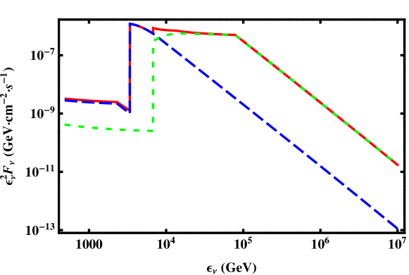
Figure 2: Neutrino flux multiplied by the square of neutrino energy versus neutrino energy for a LL-GRB. The blue dashed line represents the neutrino production through pion decay and the green dashed line is kaon decay. Meanwhile the red solid line is the total neutrino flux produced at jet head. Relevant parameters: $L_{j}=10^{42}{\rm erg\,s}^{-1}$, $\theta_{0}=0.02$, $r_{\rm He}=4\times 10^{11}{\rm cm}$, $\epsilon_{e}=\epsilon_{B}=0.1$, at a distance $D_{L}=10\,{\rm Mpc}$.

So we plot in Figure 2 the flux of neutrinos for the LL-GRB jet mentioned above, with luminosity $L_{j}=10^{42}{\rm erg\,s}^{-1}$, initial opening angle $\theta_{0}=0.02$. We assume that this LL-GRB is at a rather close distance $D_{L}=10\,{\rm Mpc}$. We can see that at low energy end, $\epsilon_{\nu}^{2}F_{\nu}\sim{\rm const}$ suggests a power law neutrino spectrum. The neutrino number from kaon decay is one or two orders of magnitude more than that from pions at high energy end. It is mainly because kaons are heavier and experience less energy loss(Horiuchi & Ando, 2008). A sharp jump is obvious in the spectrum due to the transition of dominance from the BH interaction to photopion process in proton cooling mechanisms thus prominently more neutrinos are produced, that is to say, it is caused by $\zeta_{\rm BH}(\epsilon_{\nu})$.

We now can simply estimate the neutrino events for this LL-GRB in IceCube. We use the following fitting formula of the probability of detecting muon neutrinos (Murase & Nagataki, 2006; Abbasi et al., 2011).

$$P(E_{\nu})=7\times 10^{5}(\frac{E_{\nu}}{10^{4.5}\rm GeV})^{\beta}$$

where $\beta=1.35$ for $E_{\nu}<10^{4.5}\rm GeV$, while $\beta=0.55$ for $E_{\nu}>10^{4.5}\rm GeV$. The number of muon neutrinos from a burst are given by

$$N(>E_{\nu,3})=A_{det}\int_{\rm TeV}^{\epsilon_{\nu,\max}}dE_{\nu}P(E_{\nu})\frac{dN_{\nu}(E_{\nu})}{dE_{\nu}dA}$$

Using a geometrical detector area of $A_{det}=1{\rm km}^{2}$, the expected neutrino number is $N\simeq 4.2\times 10^{-3}$ for above LL-GRB with a neutrino emission duration of $T_{dur}\simeq r_{\rm He}/\beta_{h}c\simeq 117\rm s$. Thus it is not easy to be detected now.

3.2 $1\ll\tilde{L}\lesssim\theta_{0}^{-4/3}$

In this case, the jet is still collimated but the head velocity will become subrelativistic. Similar to the above discussions, we deduce some crucial terms below,

$$\beta_{h}\simeq 1,$$

$$\tilde{L}=4(2\pi)^{-2/5}L_{j}^{2/5}A^{-2/5}\theta_{0}^{-8/5}c^{-6/5},$$

$$\Gamma_{h}=\sqrt{\frac{1}{2}}\tilde{L}^{1/4}=(2\pi)^{-1/10}L_{j}^{1/10}A^{-1/10}\theta_{0}^{-2/5}c^{-3/10},$$

$$\bar{\Gamma}_{h}=\Gamma_{j}\sqrt{\frac{1}{2}}\tilde{L}^{-1/4}=2^{-9/10}\pi^{1/10}\Gamma_{j}L_{j}^{-1/10}A^{1/10}\theta_{0}^{2/5}c^{3/10},$$

$$\theta_{j}=2^{-4/5}\pi^{-3/10}L_{j}^{3/10}A^{-3/10}\theta_{0}^{4/5}c^{-9/10},$$

$$\rho_{j}=2^{8/5}\pi^{-2/5}L_{j}^{2/5}\Gamma_{j}^{-2}A^{3/5}r^{-2}\theta_{0}^{-8/5}c^{-6/5}.$$

The internal energy of the shocked ambient medium by FS and the shocked jet by RS are

$$e_{f}=(4\Gamma_{h}+3)(\Gamma_{h}-1)\rho_{a}c^{2},\quad\quad e_{r}=(4\bar{\Gamma}_{h}+3)(\bar{\Gamma}_{h}-1)\rho_{j}c^{2}.$$

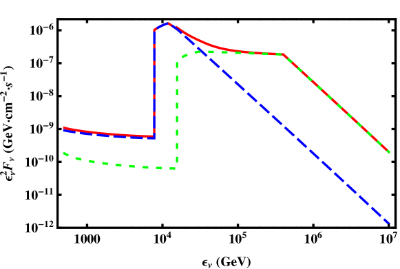
Figure 3: Neutrino flux multiplied by the square of neutrino energy versus neutrino energy, for the case of UL-GRB. The blue dashed line represents the neutrino production through pion decay and the green dashed line is kaon decay. The red solid line is the total neutrino spectrum produced at jet head. Relevant parameters: $L_{j}=2.5\times 10^{44}{\rm erg\,s}^{-1}$, $\theta_{0}=0.01$, $r_{\rm He}=5\times 10^{13}{\rm cm}$, $\epsilon_{e}=\epsilon_{B}=0.1$, at a distance $D_{L}=500\,{\rm Mpc}$.

The protons will be accelerated simultaneously by FS and RS, but the forward shock’s contribution is negligible for the reason that the FS would be radiation mediated, and the shock acceleration would be inefficient. In this case, we choose an ultra-long GRB with $L_{\rm iso}=10^{49}{\rm erg\,s}^{-1}$ and $\theta_{0}=0.01$, which suggests $L_{j}=2.5\times 10^{44}{\rm erg\,s}^{-1}$ The extreme long duration $\sim 10^{4}$s suggests a progenitor like a blue supergiant (BSG) of radii up to $\sim 10^{13}{\rm cm}$. We assume this BSG with a helium core of mass $\sim 2M_{\odot}$ and radius $r_{\rm He}=5\times 10^{13}\,$cm so that the envelope density can be expressed as $\rho_{a}(r)=6.37\times 10^{18}r^{-2}\;{\rm g\,cm}^{-3}$. The assumed radius may be relatively larger than that of typical BSG, but we choose this value in order to realize efficient Fermi acceleration here. These parameters are possible according to Woosley & Heger (2012) and then we focus on the neutrino emission of this single UL-GRB. From equation (21) we get $\tilde{L}\simeq 14.06\;,\;\rho_{j}=3.58\times 10^{-12}\;{\rm g\,cm}^{-3}\;,\;\Gamma_{h}\simeq 1.37\;,\;\bar{\Gamma}_{h}\simeq 36.5$ thus this UL-GRB satisfies $1\ll\tilde{L}\lesssim\theta_{0}^{-4/3}$. The Thomson optical depth is $\tau_{T}=n\sigma_{T}l=\frac{\rho_{j}}{m_{p}}\sigma_{T}\frac{r_{\rm He}}{\Gamma_{j}}\simeq 0.71(\frac{L_{j}}{2.5\times 10^{44}{\rm erg\,s}^{-1}})^{\frac{2}{5}}(\frac{\theta_{0}}{0.01})^{\frac{7}{5}}(\frac{M_{\rm He}}{2M_{\odot}})^{\frac{3}{5}}(\frac{r_{\rm He}}{5\times 10^{13}\rm cm})^{-\frac{8}{5}}\sim 0.1C^{-1}\bar{\Gamma}_{h}<1$ so Fermi acceleration for RS is efficient. In line with the observation now (see Gendre et al. (2013) ), we assume this UL-GRB at a relatively close distance $D_{L}=500\rm Mpc$. We calculate the neutrino flux for RS then we plot it in Figure 3. The maximum proton energy $\epsilon_{p,\max}$ can be obtained by $t_{\rm sync}=t_{\rm acc}$, and the maximum neutrino energy produced by this UL-GRB is $\epsilon_{\nu,\max}\simeq\Gamma_{h}\frac{1}{10}\epsilon_{p,\max}\simeq 3.42{\rm PeV}$. Also, Greater total neutrino fluence is exhibited in this UL-GRB case. Same as before, the expected neutrino number in IceCube for this UL-GRB is $N\simeq 8.3\times 10^{-2}$, with a neutrino emission duration of $T_{dur}\simeq r_{\rm He}/\beta_{h}c\simeq 2438\rm s$.

3.3 $\tilde{L}>\theta_{0}^{-4/3}$

This case corresponds to the uncollimated regime. That is, the collimation effect is weak and to a good approximation the jet remains conical. The head will move forward with an relativistic velocity, $\beta_{h}=1$. In this case, we have

$$\tilde{L}=\frac{L_{j}}{\pi A\theta_{0}^{2}c^{3}},$$

$$\Gamma_{h}=2^{-1/2}\pi^{-1/4}L_{j}^{1/4}A^{-1/4}\theta_{0}^{-1/2}c^{-3/4},$$

$$\bar{\Gamma}_{h}=\Gamma_{j}\sqrt{\frac{1}{2}}\tilde{L}^{-1/4},$$

$$\theta_{j}=\theta_{0},$$

$$\rho_{j}=\pi^{-1}L_{j}\Gamma_{j}^{-2}r^{-2}\theta_{0}^{-2}c^{-3}.$$

Unfortunately, this situation is not suitable for high energy neutrino production. The reason is that, to meet the requirement $\tilde{L}>\theta_{0}^{-4/3}$, we need $L_{j}=10^{53}{\rm erg\,s}^{-1}$ for $\theta_{0}=0.1$ in the helium core we previously assumed. Leaving aside the existence of such a powerful jet, the Fermi acceleration is no longer efficient and meson cooling in this jet is so severe that there will be hardly any high energy neutrinos. Hence we do not need to carry on.

4 Dependence on $\alpha$

It is reasonable to argue that the final neutrino flux depends on the density profile of progenitor envelope. Apparently, with the same assumed envelope mass and radius, different values of the power law index lead to different ambient envelope density, which directly influence the cocoon pressure and the collimation of the jet(Bromberg et al., 2011). Moreover, changing the power law index does affect the jet dynamics and result in different dependency on radius (we will see later). These two reasons cause the revision of collimation effect on the final neutrino spectrum being different. For the sake, we would like to study the influence of the different values of the power law index of the density profile. Here we display one situation (UL-GRB) for simplicity and clearness. We still use the progenitor envelope properties of a helium core of mass $\sim 2M_{\odot}$ and radius $r_{\rm He}=5\times 10^{13}{\rm cm}$, but with $\alpha=2.5,\;2.7$. Respectively, we can write them as $\rho_{a}(r)=2.25\times 10^{25}r^{-2.5}{\rm g\,cm}^{-3}$ and $\rho_{a}(r)=7.42\times 10^{27}r^{-2.7}{\rm g\,cm}^{-3}$. Surely, we could repeat all those calculations above for $\alpha=2.5,\;2.7$.

For a successful jet in the condition $1\ll\tilde{L}\lesssim\theta_{0}^{-4/3}$, we show the crucial, analytical quantities for $\alpha=2.5$,

$$\tilde{L}\simeq 2.85L_{j}^{2/5}A^{-2/5}r^{1/5}\theta_{0}^{-8/5}c^{-6/5},$$

$$\theta_{j}\simeq 0.334L_{j}^{3/10}A^{-3/10}r^{3/20}\theta_{0}^{4/5}c^{-9/10},$$

$$\rho_{j}\simeq 2.85L_{j}^{2/5}\Gamma_{j}^{-2}A^{3/5}r^{-23/10}\theta_{0}^{-8/5}c^{-6/5},$$

and for $\alpha=2.7$,

$$\tilde{L}\simeq 3.66L_{j}^{2/5}A^{-2/5}r^{7/25}\theta_{0}^{-8/5}c^{-6/5},$$

$$\theta_{j}\simeq 0.295L_{j}^{3/10}A^{-3/10}r^{21/100}\theta_{0}^{4/5}c^{-9/10},$$

$$\rho_{j}\simeq 3.66L_{j}^{2/5}\Gamma_{j}^{-2}A^{3/5}r^{-121/50}\theta_{0}^{-8/5}c^{-6/5}.$$

In all of three cases $\alpha=2,\;2.5,\;2.7$, we only consider the reverse shock’s contribution to the final high energy neutrino flux and we plot it in Figure 4. Same as before, we could get the maximum neutrino energy and it is $3.42{\rm PeV},\;4.42{\rm PeV},\;5.31{\rm PeV}$ respectively. Once we could correlate an observed high energy ($\sim\rm PeV$) neutrino precursor with a GRB in the future, we can constrain the envelope property of progenitor by maximum neutrino energy.

We can see in this figure that $\alpha$ has a visible influence on the total neutrino flux, though not so prominent. Differences occur mostly at the high energy end. Also, the energy at which the neutrino spectrum peaks and the maximum neutrino energy in these three cases are a bit different. For a steeper envelope density profile, the density of the jet material and the outer envelope at which neutrino production begins is generally smaller. Hence, the steepest $\alpha=2.7$ case encounters the least cooling impact at high energy end thus leading to a highest maximum neutrino energy and a greatest neutrino flux. Anyway, we can make this dependency more striking, for example, by choosing $\alpha=2.9$. This could result in several times distinction compared to $\alpha=2$ case at high energy end. However, given the energy resolution of IceCube now, these differences are so small that we can hardly distinguish. Here we just provide an alternative way to probe the stellar structure and wish to do this if we could realize better energy resolution in the future.

5 Comparison with Previous Works

The main calculation of our paper is based on the jet propagation dynamics developed by Bromberg et al. (2011), and we further consider the neutrino emission during the jet propagation process. This neutrino emission serves as a precursor signal prior to GRB prompt emission. We differ from Mészáros & Waxman (2001); Enberg et al. (2009); Murase & Ioka (2013) at the point that we deal with the high energy neutrino emission produced by shocks formed at the jet head, while they focused on internal shocks. We have similar handle on the calculation with Horiuchi & Ando (2008) but our result may be very different from theirs, because they adopted a progenitor model from Heger et al. (2000) with a simplified dynamics in which the jet opening angle remains constant and thus just ignored the collimation effect, which should play an important role. Collimation depends on the jet luminosity $L_{j}$, initial opening angle $\theta_{0}$ and the progenitor density profile. We calculate in detail the high energy neutrino flux in each collimation regime, and choose the promising LL-GRBs and UL-GRBs as high energy neutrino sources, leading to a more likely result. And what is more, we discuss the dependence of maximum neutrino energy and high energy neutrino flux on the progenitor density profile.

6 Discussions and Conclusions

High energy neutrinos can be produced while the jet is still propagating in the envelope. These neutrinos appear as a precursor signal, with energy ranges from GeV to PeV. Analytically, we calculate this neutrino flux. To handle this, we first need to determine whether the jet is in collimation regime. Collimation has a crucial effect on jet propagation dynamics. We adopt the previous propagation framework developed by Bromberg et al. (2011). We assume separated cases (LL-GRBs and UL-GRBs) in which Fermi first order acceleration works and they fall into different collimation regimes. With a power law spectrum of accelerated protons with $p=2$, then we calculate the neutrino flux in various situations.

At low energy end, we always get $\epsilon_{\nu}^{2}F_{\nu}\sim{\rm const}$ and this suggests a power law neutrino spectrum. Neutrinos are mainly produced by proton-proton collision. As the neutrino energy goes higher, a sharp jump is obvious in the spectrum because of photopion process starting to dominate thus more neutrinos are expected. Moreover, the neutrino flux from kaon decay is almost two orders of magnitude more than that from pions at high energy end. It is mainly because kaons are heavier and experience less energy loss.

In our expectation, the final neutrino flux will depend on the density profile parameter $\alpha$. We take $\alpha=2,\;2.5,\;2.7$ to verify this dependence. We get a good result in Figure 4, which shows that the dependence is existing. Besides, the maximum neutrino energy for three cases is $3.42{\rm PeV},\;4.42{\rm PeV},\;5.31{\rm PeV}$ respectively. At a given radius, the density of the jet material is lower for a steeper envelope density profile. There is less cooling impact so that a higher maximum neutrino energy and a greater high energy neutrino flux is expected.

In this paper, we only calculate the high energy neutrino flux of one GRB for given parameters, but it is not easy to be detected by the current instruments. We wish to obtain a diffuse GRB neutrino background which can be correlated with current observations in our future work.

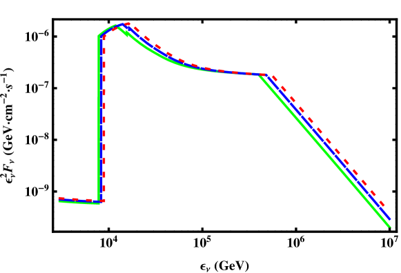
Figure 4: Total neutrino flux multiplied by the square of neutrino energy versus neutrino energy for a UL-GRB with different envelope density profile. Green solid lines, blue dashed lines and red dotted lines represent $\alpha=2$, $\alpha=2.5$, $\alpha=2.7$ respectively. Relevant parameters: $L_{j}=2.5\times 10^{44}{\rm erg\,s}^{-1}$, $\theta_{0}=0.01$, $r_{\rm He}=5\times 10^{13}{\rm cm}$, $\epsilon_{e}=\epsilon_{B}=0.1$, at a distance $D_{L}=500\,{\rm Mpc}$.

References

- Abbasi et al. (2011) Abbasi, R. et al. (IceCube Collaboration) 2011, Phys. Rev. D, 83, 012001
- Achterberg et al. (2001) Achterberg, A., Gallant, Y. A., Kirk, J. G., & Guthmann, A. W. 2001, MNRAS, 328, 393
- Ando & Beacom (2005) Ando, S., Beacom, J. F. 2005, Phys. Rev. Lett., 95, 061103
- Ando et al. (2005) Ando, S., Beacom, J. F., & Yuksel, H. 2005, Phys. Rev. Lett., 95, 171101
- Alvarez-Muniz et al. (2000) Alvarez-Muniz, J., Halzen, F., & Hooper, D. W. 2000, Phys. Rev. D, 62, 093015
- Asano (2005) Asano, K. 2005, ApJ, 623, 967
- Bahcall & Waxman (2001) Bahcall, J., & Waxan, E. 2001, Phys. Rev. D, 64, 023002
- Becker (2008) Becker, J. K. 2008, Phys. Rep., 458, 173
- Begelman & Cioffi (1989) Begelman, M. C., & Cioffi, D. F. 1989, ApJ, 345, L21
- Blandford & McKee (1976) Blandford, R. D., & McKee, C. F. 1976, Phys. Fluids., 19, 1130
- Bromberg et al. (2011) Bromberg, O., Nakar, E., Piran, T., & Sari, R. 2011, ApJ, 740, 100
- Budnik et al. (2010) Budnik, R., Katz, B., Sagiv, A., & Waxman, E. 2010, ApJ, 725, 63
- Dai & Lu (2001) Dai, Z. G., & Lu, T. 2001, ApJ, 551, 249
- Dermer et al. (2003) Dermer, C. D., & Atoyan, A. 2003, Phys. Rev. Lett., 91, 071102
- Eidelman et al. (2004) Eidelman, S. et al. [Particle Data Group], 2004, Phys. Rev. B, 592, 1
- Enberg et al. (2009) Enberg, R., Reno, M. H., & Sarcevic, I. 2009, Phys. Rev. D, 79, 053006
- Gao et al. (2012) Gao, S., Asano, K., & Mészáros, P. 2012, JCAP, 1211, 058
- Gendre et al. (2013) Gendre, B. et al. 2013, ApJ, 766, 30
- Guetta & Granot (2003) Guetta, D., & Granot, J. 2003, Phys. Rev. Lett., 90, 201103
- Guetta et al. (2004) Guetta, D., Hooper, D., Alvarez-Muñiz, J., Halzen, F., & Reuveni, E. 2004, Astroparticle Physics, 20, 429
- Heger et al. (2000) Heger, A., Langer, N. & Woosley, S. E. 2000, ApJ, 528, 368
- Horiuchi & Ando (2008) Horiuchi, S., & Ando, S. 2008, Phys. Rev. D, 77, 063007
- Katz et al. (2010) Katz, B., Budnik, R., & Waxman, E. 2010, ApJ, 716, 781
- Keshet & Waxman (2005) Keshet, U., & Waxman, E. 2005, Phys. Rev. Lett., 94, 111102
- Lazzati & Begelman (2005) Lazzati, D., & Begelman, M. 2005, ApJ, 629, 903
- Levinson & Bromberg (2008) Levinson, A., & Bromberg, O. 2008, Phys. Rev. Lett., 100, 131101
- Levan et al. (2013) Levan, A. J. et al. 2013, arXiv:1302.2352.
- Li et al. (2002) Li, Z., Dai, Z. G., & Lu, T. 2002, A&A, 396, 303
- Liang et al. (2007) Liang, E., Zhang, B., Francisco, V., & Dai, Z. G. 2007, ApJ, 662, 1111L
- MacFadyen & Woosley (1999) MacFadyen, A., & Woosley, S. E. 1999, ApJ, 524, 262
- Matzner (2003) Matzner, C. D. 2003, MNRAS, 345, 575
- Mészáros & Rees (2000) Mészáros, P., & Rees, M. J. 2000, ApJ, 541, L5-L8
- Mészáros & Waxman (2001) Mészáros, P., & Waxman, E. 2001, Phys. Rev. Lett., 87, 171102
- Mészáros (2006) Mészáros, P. 2006, Rept. Prog. Phys., 69, 2259
- Mizuta & Aloy (2009) Mizuta, A., & Aloy, M. A. 2009, ApJ, 699, 1261
- Mizuta & Ioka (2013) Mizuta, A., & Ioka, K. 2013, ApJ, 777, 162
- Morsony et al. (2007) Morsony, B. J., Lazzati, D., & Begelman, M. C. 2007, ApJ, 665, 569
- Murase et al. (2006) Murase, K., Ioka, K., Nagataki, S., &Nakamura, T. 2006, ApJ, 651, L5
- Murase & Nagataki (2006) Murase, K., & Nagataki, S. 2006, Phys. Rev. D, 73, 063002
- Murase (2007) Murase, K. 2007, Phys. Rev. D, 76, 123001
- Murase (2008) Murase, K. 2008, Phys. Rev. D, 78, 101302
- Murase & Ioka (2013) Murase, K., & Ioka, K. 2013, Phys. Rev. Lett., 111, 121102
- Nakar & Sari (2012) Nakar, E. & Sari, R. 2012, ApJ, 747, 88
- Piran (2005) Piran, T. 2005, Rev. Mod. Phys., 76, 1143
- Pruet (2003) Pruet, J. 2003, ApJ, 591, 1104-1109
- Rachen & Mészáros (1998) Rachen, J. P., & Mészáros, P. 1998, Phys. Rev. D, 58, 123005
- Razzaque et al. (2003) Razzaque, S., Mészáros, P., & Waxman, E. 2003, Phys. Rev. D, 68, 083001
- Razzaque et al. (2003) Razzaque, S., Mészáros, P., & Waxman, E. 2003, Phys. Rev. Lett., 90, 241103
- Razzaque et al. (2004) Razzaque, S., Mészáros, P., & Waxman, E. 2004, Phys. Rev. Lett., 93, 181101
- Razzaque (2013) Razzaque, S. 2013, Phys. Rev. D, 88, 103003
- Rees & Mészáros (2005) Rees, M. J., & Mészáros, P. 2005, ApJ, 628, 847
- Sari & Piran (1995) Sari, R., & Piran, T. 1995, ApJ, 455, L143
- Soderberg et al. (2006) Soderberg, A. M. et al. 2006, Nature (London) 442, 1014
- Stecker (1968) Stecker, F. W. 1968, Phys. Rev. Lett., 21, 1016
- Toma et al. (2007) Toma, K., Ioka, K., Sakamoto, T. & Nakamura, T. 2007, ApJ, 659, 1420
- Totani (2003) Totani, T. 2003, ApJ, 598, 1151
- Vietri (1995) Vietri, M. 1995, ApJ, 453, 883
- Wang & Dai (2009) Wang, X. Y., & Dai, Z. G. 2009, ApJ, 691, 67
- Waxman & Bahcall (1997) Waxman, E., & Bahcall, J. 1997, Phys. Rev. Lett., 78, 2292
- Waxman & Bahcall (1999) Waxman, E., & Bahcall, J. 1998, Phys. Rev. D, 59, 023002
- Waxman & Bahcall (2000) Waxman, E., & Bahcall, J. 2000, ApJ, 541, 707
- Woosley (1993) Woosley, S. E. 1993, ApJ, 405, 273
- Woosley & Heger (2006) Woosley, S. E., & Heger, A. 2006, ApJ, 637, 914
- Woosley & Heger (2012) Woosley, S. E., & Heger, A. 2012, ApJ, 752, 32
- Zhang & Mészáros (2004) Zhang, B., & Mészáros, P. 2004, Int. J. Mod. Phys. A 19, 2385
- Zhang et al. (2003) Zhang, W., Woosley, S. E., & MacFadyen, A. 2003, ApJ, 586, 356