Renormalization and forcing of Horseshoe Orbits

Abstract.

In this paper we deal with the Boyland order of horseshoe orbits. We prove that there exists a set $\mathcal{R}$ of renormalizable horseshoe orbits containing only quasi-one-dimensional orbits, that is, for these orbits the Boyland order coincides with the unimodal order.

1. Introduction

In [2], Boyland introduced the forcing relation between periodic orbits of the disk $D^{2}$. Given two periodic orbits $P$ and $R$, we say that $P$ forces $R$, denoted by $P\geqslant_{2}R$, if every homeomorphism of $D^{2}$ containing the braid type of $P$ must contain the braid type of $R$. The set of periodic orbits forced by $P$ is denoted by $\Sigma_{P}$. In this paper we are concerned with the forcing of Smale horseshoe periodic orbits. A horseshoe orbit $P$ is called quasi-one-dimensional if $P$ forces all orbit $R$ such that $P\geqslant_{1}R$, where $\geqslant_{1}$ is the unimodal order. In [4], Hall gave a set of quasi-one-dimensional horseshoe orbits, called NBT orbits (Non-Bogus Transition orbits) which are in bijection with $\mathbb{Q}\cap(0,\frac{1}{2})$ and have the property that their thick interval map induced has minimal periodic orbit structure, that is, if $P$ is an NBT orbit then every braid type of a periodic orbit of its thick interval map $\theta_{P}$ is forced by the braid type of $P$.

In this paper we obtain a type of orbits which are quasi-one-dimensional too although their associated thick interval maps are reducible in the sense of Thurston [6], that is, they are isotopic to reducible homeomorphisms which have an invariant set of non-homotopically trivial disjoint curves $\{C_{1},\cdots,C_{n}\}$. Restricted to the components of $D^{2}\setminus\{C_{1},\cdots,C_{n}\}$, these reducible maps (or one of its power) have minimal periodic orbit structure.

Theorem 1.

There exists a set $\mathcal{R}\supset\operatorname{NBT}$ of quasi-one-dimensional horseshoe orbits, that is, if $P\in\mathcal{R}$ then $\Sigma_{P}=\{R:P\geqslant_{1}R\}$.

These orbits are defined using the renormalization operator which was introduced in [3] as the $*$-product.

2. preliminaries

2.1. Boyland partial Order

Let $D_{n}$ be the punctured disk. Let $\operatorname{MCG}(D_{n})$ be the group of isotopy classes of homeomorphisms of $D_{n}$, which is called the mapping class group of $D_{n}$. Given a homeomorphism $f:D^{2}\rightarrow D^{2}$ of the disk $D^{2}$ with a periodic orbit $P$, the braid type of $P$, denoted by $\operatorname{bt}(P,f)$, is defined as follows: Take an orientation preserving homeomorphism $h:D^{2}\setminus P\rightarrow D_{n}$ then $\operatorname{bt}(P,f)$ is the conjugacy class $[h\circ f\circ h^{-1}]\in\operatorname{MCG}(D_{n})$ of $h\circ f\circ h^{-1}:D_{n}\rightarrow D_{n}$.

Let $\operatorname{BT}$ be the union of all the periodic braid types and let $\operatorname{bt}(f)$ be the set formed by the braid types of the periodic orbits of $f$. We will say that $f:D^{2}\rightarrow D^{2}$ exhibits a braid type $\beta$ if there exists an $n$-periodic orbit $P$ for $f$ with $\beta=\operatorname{bt}(P,f)$. Now we can define the relation $\geqslant_{2}$ on $\operatorname{BT}$. We say that $\beta_{1}$ forces $\beta_{2}$, denoted by $\beta_{1}\geqslant_{2}\beta_{2}$, if every homeomorphism exhibiting $\beta_{1}$, exhibits $\beta_{2}$ too. Then it is said that a periodic orbit $P$ forces another periodic orbit $R$, denoted by $P\geqslant_{2}R$, if $\operatorname{bt}(P)\geqslant_{2}\operatorname{bt}(R)$.

In [2], P. Boyland proved the following theorem.

Theorem 2.

[2, Theorem 9.1] The relation $\geqslant_{2}$ is a partial order.

2.2. Smale horseshoe

The Smale horseshoe is a map $F:D^{2}\rightarrow D^{2}$ of the disk which acts as in Fig. 1. The set $\Omega=\cap_{j\in\mathbb{Z}}F^{j}(V_{0}\cup V_{1})$ is $F$-invariant and $F|_{\Omega}$ is conjugated to the shift $\sigma$ on the sequence space of two symbols $0$ and $1$, $\Sigma_{2}=\{0,1\}^{\mathbb{Z}}$, where

(1) $$\sigma((s_{i})_{i\in\mathbb{Z}})=(s_{i+1})_{i\in\mathbb{Z}}.$$

The conjugacy $h:\Omega\rightarrow\Sigma_{2}$ is defined by

(2) $$(h(x))_{i}=\left\{\begin{array}[]{cc}0&\textrm{ if }F^{i}(x)\in V_{0},\\ 1&\textrm{ if }F^{i}(x)\in V_{1}.\\ \end{array}\right.$$

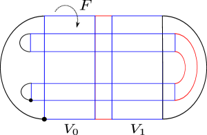
Figure 1. Dynamics of $F$.

To compare horseshoe orbits it is necessary to define the unimodal order. It is a total order in $\Sigma^{+}=\{0,1\}^{\mathbb{N}}$ given by the following rule: Let $s=s_{0}s_{1}...$ and $t=t_{0}t_{1}...$ be sequences in $\Sigma^{+}$ such that $s_{i}=t_{i}$ for $i\leq k$ and $s_{k+1}\neq t_{k+1}$, then $s<t$ if

• $\sum_{i=0}^{k}s_{i}$ is even and $s_{k+1}<t_{k+1}$, or

• $\sum_{i=0}^{k}s_{i}$ is odd and $s_{k+1}>t_{k+1}$.

We say that $s\geqslant_{1}t$ if either $s=t$ or $s>t$.

Every $n$-periodic orbit $P\in\Omega$ of $F$ has a code denoted by $c_{P}\in\Sigma_{2}$. It is obtained from $h(p)=c_{P}^{\infty}$ where $p$ is a point of $P$ and $c_{P}$ satisfies $\sigma^{i}(c_{P})\leqslant_{1}c_{P}$, that is, $c_{P}$ is maximal in the unimodal order $\geqslant_{1}$. We say that $P\geqslant_{1}R$ if $\sigma^{n}(R)\leqslant_{1}c_{P}$, $\forall n\geq 1$. For every orbit $P$, there exists a homeomorphism $\theta_{P}$ that realizes the combinatorics of $P$. This is obtained fatting the line diagram of $P$ and it is called the tick map induced by $P$. See [4].

2.3. Renormalized Horseshoe Orbits

Let $P$ and $Q$ be two horseshoe periodic orbits with codes $c_{P}=Aa_{n-1}$ where $A=a_{0}a_{1}\cdots a_{n-2}$ and $c_{Q}=b_{0}b_{1}\cdots b_{m-2}b_{m-1}$ with periods $n$ and $m$, respectively.

Definition 3 (Renormalization Operator).

We will write $P*Q$ for the $nm$-periodic orbit with code

(3) $$c_{P*Q}=\left\{\begin{array}[]{cc}Ab_{0}Ab_{1}Ab_{2}\cdots Ab_{m-2}Ab_{m-1}&\textrm{ if }\epsilon(A)\textrm{ is even}\\ A\overline{b_{0}}A\overline{b_{1}}A\overline{b_{2}}\cdots A\overline{b_{m-2}}A\overline{b_{m-1}}&\textrm{ if }\epsilon(A)\textrm{ is odd}\\ \end{array}\right.$$

where $\epsilon(A)=\sum_{i=0}^{n-2}a_{i}$ and $\overline{b_{i}}=1-b_{i}$.

The orbit $P*Q$ is called the renormalization of $P$ and $Q$. If an orbit $S$ satisfies $S=P*Q$ for some $P,Q\in\Sigma_{2}$, it is said that $S$ is renormalizable. Also we will denote

$$P_{1}*P_{2}*\cdots*P_{k}=(\cdots((P_{1}*P_{2})*P_{3})\cdots).$$

Example 4.

If $P=101$ and $Q=1001$ then $P*Q=10\mathbf{0}10\mathbf{1}10\mathbf{1}10\mathbf{0}$.

2.4. NBT Orbits

There are a type of horseshoe orbits for which the Boyland partial order is well-understood. They are constructed in the following way. Given a rational number $q=\frac{m}{n}\in\widehat{\mathbb{Q}}:=\mathbb{Q}\cap(0,\frac{1}{2})$, let $L_{q}$ be the straight line segment joining $(0,0)$ and $(n,m)$ in $\mathbb{R}^{2}$. Then construct a finite word $c_{q}=s_{0}s_{1}\cdots s_{n}$ as follows:

(4) $$s_{i}=\left\{\begin{array}[]{cc}1&\textrm{ if $L_{q}$ intersects some line $y=k,k\in\mathbb{Z}$, for $x\in(i-1,i+1)$}\\ 0&\textrm{ otherwise }\\ \end{array}\right.$$

It follows that $c_{q}$ is palindromic and has the form:

(5) $$c_{q}=10^{\mu_{1}}1^{2}0^{\mu_{2}}1^{2}\cdots 1^{2}0^{\mu_{m-1}}1^{2}0^{\mu_{m}}1.$$

We will denote $P_{q}$ to the periodic orbits of period $n+2$ which have the codes $c_{q}{}_{0}^{1}$, when the distinction is not important and let $\operatorname{NBT}=\{P_{q}:q\in\widehat{\mathbb{Q}}\}$. In [4], Hall proved the following result.

Theorem 5.

Let $q,q^{\prime}\in\widehat{\mathbb{Q}}$. Then

• $P_{q}$ is quasi-one-dimensional, that is, $P_{q}\geqslant_{1}R\Longrightarrow P_{q}\geqslant_{2}R$.

• $q\leqslant q^{\prime}\Longleftrightarrow(c_{q}{}^{0}_{1})^{\infty}\geqslant_{1}(c_{q^{\prime}}{}^{0}_{1})^{\infty}\Longleftrightarrow(c_{q}{}^{0}_{1})^{\infty}\geqslant_{2}(c_{q^{\prime}}{}^{0}_{1})^{\infty}$

So theorem above says that the Boyland order restricted to the NBT orbits is equal to the unimodal order.

3. Forcing of renormalizable orbits

For proving Theorem 1 we need the following result:

Theorem 6.

Let $P=A_{1}^{0}$ and $Q$ be periodic orbits. Then

(6) $$\Sigma_{P*Q}=\{R:P\geqslant_{2}R\}\cup\{P*R:Q\geqslant_{2}R\}.$$

To prove the result above it will be needed two lemmas whose proofs are left to the reader.

Lemma 7.

Let $i,j\in\{1,\cdots,n-1\}$ be positive integers with $i\neq j$ and $T_{M}=P*Q$ and $T_{m}=\sigma^{n}(T_{M})$. Then

• if $\epsilon(A)$ is even then $A0^{\infty}\leqslant_{1}T_{m}\leqslant_{1}T_{M}\leqslant_{1}A1^{\infty}$,

• if $\epsilon(A)$ is odd then $A1^{\infty}\leqslant_{1}T_{m}\leqslant_{1}T_{M}\leqslant_{1}A0^{\infty}$,

• $\sigma^{i}(P)\leqslant_{1}\sigma^{j}(P)\Longleftrightarrow[\sigma^{i}(T_{M})\leqslant_{1}\sigma^{j}(T_{M})\textrm{ and }\sigma^{i}(T_{m})\leqslant_{1}\sigma^{j}(T_{m})]$.

Lemma 8.

Let $P=A{}_{1}^{0}$ and $Q$ be two periodic orbits. If $i,j\in\{0,\cdots,m-1\}$, with $i\neq j$, then

$$\sigma^{i}(Q)>_{1}\sigma^{j}(Q)\Longleftrightarrow\sigma^{in}(P*Q)>_{1}\sigma^{jn}(P*Q).$$

Proof of Theorem 6.

Let $\theta_{P*Q}$ be the thick map induced by $P*Q$. First we see that the only iterates of $P*Q$ satisfying $T_{m}\leqslant_{1}\sigma^{i}(P*Q)\leqslant_{1}T_{M}$ are the iterates $\sigma^{in}(P*Q)$, with $0\leq i\leq m-1$; so there exists a curve $C_{n-1}$ containing these orbits disjoint from the others and bounding a region $D_{n-1}$. By Lemma 7(c) and noting that $\sigma^{i}(T_{m})$ and $\sigma^{i}(T_{M})$ has the same initial symbol for $i\in\{1,\cdots,n-1\}$, it follows that $\{\theta_{P*Q}^{i}(C_{n-1})\}_{i=1}^{n-1}$ has the same combinatorics as $P$. For $i=0,\cdots,n-2$, let $C_{i}=\theta_{P*Q}^{i+1}(C_{n-1})$ be a curve which bounds a domain $D_{i}$. It is possible to define $\theta_{P*Q}$ such that $\theta_{P*Q}^{n}(C_{n-1})=C_{n-1}$. Then the line diagram of $\{D_{0},\cdots,D_{n-1}\}$ is as the line diagram of $P$ and then $\theta_{P*Q}$ has the same behaviour than $\theta_{P}$ in the exterior of $\cup D_{i}$. Since $\theta_{P*Q}$ can be reduced by a family of curves, we will need study the Thurston representative of $\theta_{P*Q}$ restricted to $D^{2}\setminus\cup C_{i}$. As $\theta_{P}$ and $\theta_{P*Q}$ have the same combinatorics in the exterior of $\cup D_{i}$, they have the same Thurston representative in the exterior of $\cup D_{i}$. So $P$ and $P*Q$ force the same periodic orbits in the exterior of $\cup D_{i}$. Then $\{R:P\geqslant_{2}R\}\subset\Sigma_{P*Q}$. See Fig. 2.

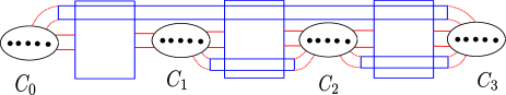
Figure 2. The image $\theta_{P*Q}(C_{i})$ when $P=1001$.

It is clear that to find what orbits are forced by $P*Q$ in $\cup D_{i}$, it is enough to study $\theta_{P*Q}^{n}$ restricted to $D_{n-1}$. By Lemma 8, the line diagram of $\theta_{P*Q}^{n}$ inside $D_{n-1}$ is the same as the line diagram of $Q$ when $\epsilon(A)$ is even, and it is flipped when $\epsilon(A)$ is odd. See Fig. 3(b). So $\theta_{P*Q}^{n}$ has the same combinatorics than $\theta_{Q}$.

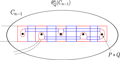
(a) When $\epsilon(A)$ is even and $Q=10010$.

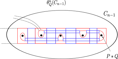
(b) When $\epsilon(A)$ is odd and $Q=10010$.

Figure 3. The image $\theta_{P*Q}^{n}(C_{n-1})$.

As in Lemma 8, we can prove that $R\leqslant_{2}Q\Longleftrightarrow P*R\leqslant_{2}P*Q.$ So $\Sigma_{P*Q}=\{R:P\geqslant_{2}R\}\cup\{P*R:Q\geqslant_{2}R\}$. ∎

Remark 9.

Theorem 6 says us that to look for the orbits that are forced by $P*Q$ it is enough to look for the orbits that are forced by $P$ and the orbits that are forced by $Q$. So we can study the thick maps induced by $P$ and $Q$ separately. Every of these thick maps can be reduced using methods to determine its minimal representative, e.g. [1, 5].

Corollary 10.

Let $P_{1},P_{2},\cdots,P_{k}$ be NBT orbits. Then

• $\Sigma_{P_{1}*\cdots*P_{k}}=\cup_{j=1}^{k}\{P_{1}*\cdots*P_{j-1}*R:P_{j}\geqslant_{1}R\}$

• $\Sigma_{P_{1}*\cdots*P_{k}}=\{R:P_{1}*\cdots*P_{k}\geqslant_{1}R\}$

Proof.

Item (a) follows directly from Theorem 6. For item (b) it is enough to prove that if $P$ and $Q$ are quasi-one-dimensional horseshoe orbits then $P*Q$ is a quasi-one-dimensional orbit too. Suppose that $\epsilon(A)$ is even. From Theorem 6,

(7) $$\Sigma_{P*Q}=\{R:P\geqslant_{1}R\}\cup\{P*R:Q\geqslant_{1}R\}.$$

Hence it follows that $\Sigma_{P*Q}\subset\{S:P*Q\geqslant_{1}S\}$. We have to prove the inclusion $\{S:P*Q\geqslant_{1}S\}\subset\Sigma_{P*Q}$. If $P\geqslant_{1}S$ then $S\in\Sigma_{P*Q}$. Let $S$ with $c_{S}=s_{0}s_{1}\cdots s_{k-1}$ be a periodic orbit with $P\leqslant_{1}S\leqslant_{1}P*Q$. By Lemma 7(a), $(A0){}^{\infty}\leqslant_{1}c_{S}^{\infty}\leqslant_{1}(A1){}^{\infty}$. This implies that $c_{S}=As_{n-1}s_{n}\cdots$ and

$$(0A)^{\infty}\leqslant_{1}\sigma^{n-1}(c_{S}^{\infty})=s_{n-1}s_{n}\cdots\leqslant_{1}(1A)^{\infty},$$

and $\sigma^{n}(c_{S}{}^{\infty})\geqslant_{1}(A0)^{\infty}$. In the other hand $\sigma^{n}(c_{S}{}^{\infty})\leqslant_{1}c_{P*Q}{}^{\infty}$. Then $\sigma^{n}(c_{S}{}^{\infty})=As_{2n-1}\cdots$ and then $c_{S}=As_{n}As_{2n-1}\cdots$. Continuing this process, it follows that $S=P*R$ where $c_{R}=s_{n-1}s_{2n-1}\cdots$. So $P*R\leqslant_{1}P*Q$ which implies that $R\leqslant_{1}Q$. So $S\in\{P*R:Q\geqslant_{1}R\}$ and the proof is finished.

∎

Now we proceed to prove Theorem 1.

Proof of Theorem 1.

Let $\{P_{j}\}_{j\in\mathbb{N}}$ be the set of NBT orbits and consider the space $\mathbb{N}^{\mathbb{N}}$ of sequences of positive integers. Take a sequence $\mathcal{J}=(j_{1},j_{2},\cdots,j_{n},\cdots)\in\mathbb{N}^{\mathbb{N}}$ and define

(8) $$\mathcal{R}_{\mathcal{J}}=\cup_{k=1}^{\infty}\{P_{j_{1}}*\cdots*P_{j_{k}}\}$$

and $\mathcal{R}=\cup_{\mathcal{J}\in\mathbb{N}^{\mathbb{N}}}\mathcal{R}_{\mathcal{J}}$. By Corollary 10(b), every orbit of $\mathcal{R}$ is quasi-one-dimensional. ∎

Example 11.

By previous Theorem, if $S=10010*10010=1001\mathbf{1}1001\mathbf{0}1001\mathbf{0}1001\mathbf{1}1001\mathbf{0}$,

(9) $$\Sigma_{S}=\{R:10010\geqslant_{1}R\}\cup\{10010*R:10010\geqslant_{1}R\}.$$

4. acknowledgements

I would like to thank to Toby Hall and Dylene de Barros for their comments which contributed to improve this paper.

References

[1]Bestvina, M. and Handel, M.:
Train-Tracks for Surface homeomorphisms.
Topology, 34, 109–140 (1995).
[2]Boyland, P.:
Topological methods in surface dynamics.
Topology and its Applications, 54, 223–298 (1994).
[3]Collet, P. and Eckmann, J-P.:
Iterated Maps on the Interval as Dynamical Systems. Birkhauser, Boston (1980).
[4]Hall, T.:
The creation of horseshoes. Nonlinearity,
7, 861–924 (1994).
[5]Solari, H. and Natiello, M.:
Minimal periodic orbits structure of 2-dimensional homeomorphisms.
Journal of Nonlinear Science, 15(3), 183–222 (2005).
[6]Thurston, W.:
On the geometry and dynamics of diffeomorphisms of surface.
Bull. Amer. Math. Soc. (N. S.), 19, 417–431 (1988).